Observing Water Surface Temperature from Two Different Airborne Platforms over Temporarily Flooded Wadden Areas at the Elbe Estuary—Methods for Corrections and Analysis

Abstract

Over the Hahnöfer Nebenelbe, a part of the Elbe estuary near Hamburg, Germany, a combined aerial survey with an unmanned aerial system (UAV) and a gyrocopter was conducted to acquire information about the water surface temperatures. The water temperature in the estuary is important for biological processes and living conditions of riverine organisms. This study aimed to develop a workflow that allows for comparing and analysing surface temperatures acquired by two different remote sensing systems. The thermal infrared (TIR) datasets were compared with in situ measurements gathered during the data acquisition, where both TIR datasets showed a varying bias. Potential error sources regarding the absolute and relative accuracy were investigated and modelled based on the available measurements, including emissivity, atmosphere, skin effect at the water surface, camera flat field correction and calibration. The largest effects on the observed TIR water temperature had the camera calibration and the modelled atmospheric effects. After the correction steps, both datasets could be combined to create a multitemporal representation of the temperature pattern and profiles over the survey area’s wadden flats.

1. Introduction

The Elbe estuary is a mesotidal system with high temporal and spatial variability, where water quality parameters can change quickly over time during the tide and over short distances between the main fairway, side channels and intertidal mudflats. Water temperature is an important water quality parameter and serves as an indicator of dissolved oxygen content [1,2] which is in turn important for ecosystem and living conditions of riverine organisms. The distribution of water temperatures and mixing processes of water bodies in the Elbe estuary depend on the interaction of the tide and river flow with the topography (location of islands and channels, shallow areas and wadden flats), and the atmospheric conditions, especially insolation and wind [3]. For an overview as complete as possible, measurements have to be conducted at several points during the tidal cycle and at a high spatial resolution. This study aims to evaluate the potential of airborne thermal infrared (TIR) imagers to measure water surface temperature during the tide and develop the necessary methodology for their correction and analysis. The TIR data sets are intended to evaluate temperature patterns over tidal mudflats and to validate a water quality model of the Elbe estuary, QSim [4,5].

Water surface temperature or sea surface temperature (SST) acquired by satellite data has been used frequently due to its availability for investigating boundary currents, studying fish and wildlife habitats, monitoring climate change (on a large scale) and coastal upwelling, where rising cold water brings nutrients to the surface [6]. Satellite SSTs are also able to general map patterns and extensions of thermal plume signatures in coastal areas [7], monitor heated effluent discharge from the nuclear power plant [8] or to reconstruct river surface temperature and turbidity regimes of an estuary [9]. However, for the aim of this study, their acquisition rate is too infrequent for resolving the tidal cycle, and the spatial resolution is too coarse.

Alternatively, thermal infrared (TIR) cameras on other platforms have been used for inland water streams and waterways. The absolute accuracy of uncooled, lightweight thermal sensors is low (typically $\pm 2{}^{\circ }$C/$\pm 2\%$) compared to in situ measurements (±0.1 ${}^{\circ }$C), thermal radiometry (±0.2 ${}^{\circ }$C) [10] or calibrated thermal airplane or satellite sensors (±0.1 ${}^{\circ }$C). However, they have been often utilized where temperature patterns are relevant: to assess cold-water reservoirs and thermal refuges [11,12], to locate groundwater inputs and hyporheic upwelling [13], to acquire maps of thermal heterogeneity and water surface temperature longitudinally and laterally across stream channel, river channels and wadden flats [12,14,15,16,17]. In coastal areas, aerial TIR data acquired by small airplanes or unmanned aerial vehicles have proven to be an efficient method for mapping submarine groundwater discharge [18,19,20,21,22].

When mapping the thermal landscape, the water temperature patterns fluctuating over time and varying on the river network [23], fine-scale continuous temperature measurements are necessary to acquire the complete signal of the data, not only mean, minimum or maximum water temperatures [14,23]. Wawrzyniak et al. [24] have shown that it is also possible to use this method for a larger spatial scale and several time points and measured patterns of diel fluctuations of water temperature.

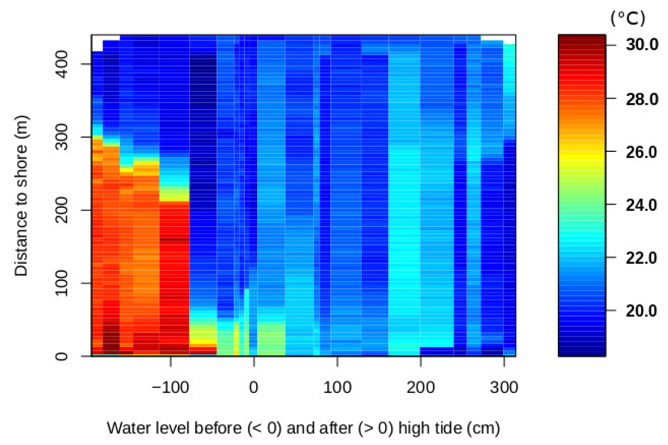
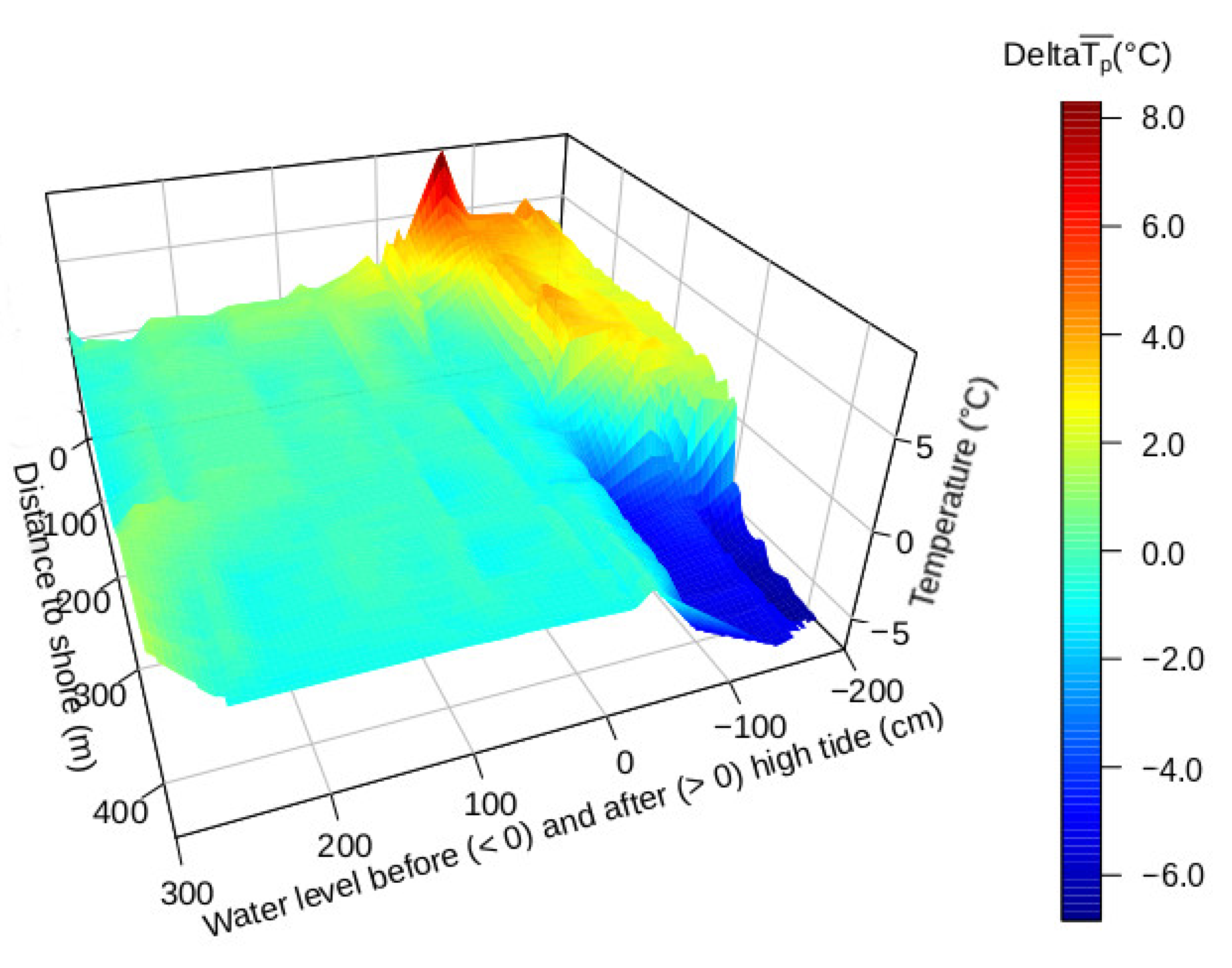
In this research survey, the particular temporal and spatial element of interest within the thermal landscape, the investigated facet [23], are the wadden flats/intertidal mudflats and how the water temperature changes during high and low tide. Here, the largest temperature differences are expected when the overflowing water is heated during the day and flowing in the stream channel during low tide. In 2014, in situ temperature measurements have shown that during the summer, distinctive temperature differences of about 1.5 ${}^{\circ }$C can occur between the water in channels and over the mudflats as soon as the mudflats are covered with water despite the frequent flooding and water movement during the tides. However, the measurements in the mudflats were complicated by the fluctuating water levels and a limited number of in situ measurement locations, which allowed for only a limited picture of the water movement and mixing processes. Hence, the aim of this research study was (i) to test tools and platforms (specifically a gyrocopter and a hexacopter) to acquire water surface temperature patterns of the intertidal mudflats during high tide at a high spatial and temporal resolution, (ii) to develop a processing workflow for correction and to achieve a high relative and absolute accuracy and (iii) to derive temperature products that allow for an in-depth analysis of mixing processes as well as comparison with results of the water quality model QSim. A specific aspect of this survey was also the use of low-cost platforms and thermal imagers to minimize the actual costs of data acquisition and to allow for potential regular monitoring in the future.

After the data acquisition description follows the analysis of potential error sources on the derived surface temperatures and necessary correction steps. These correction steps include an emissivity correction, atmospheric correction, flat field correction of the UAV camera, and in situ calibration. In the end, examples of the acquired thermal landscapes are presented and discussed.

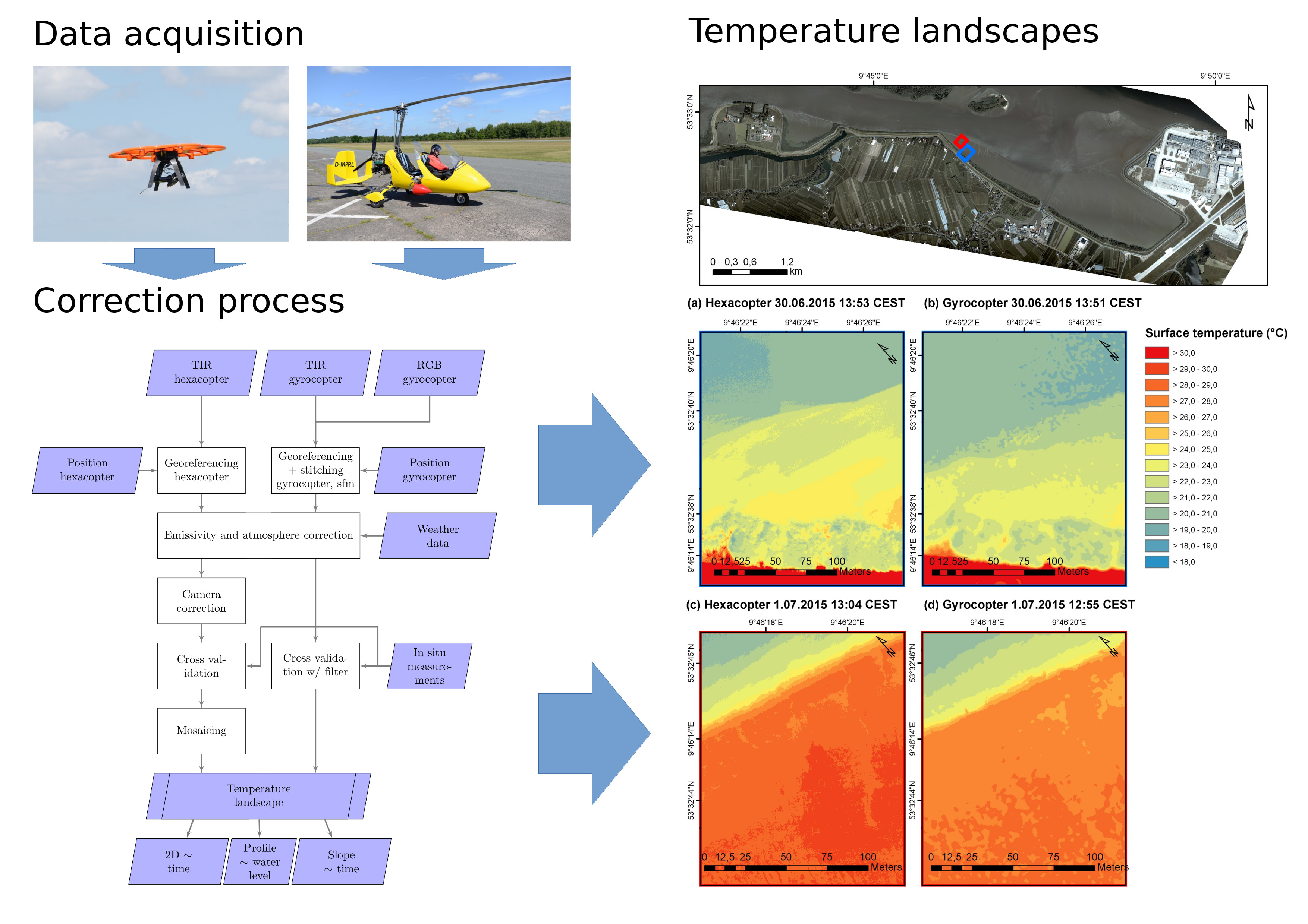
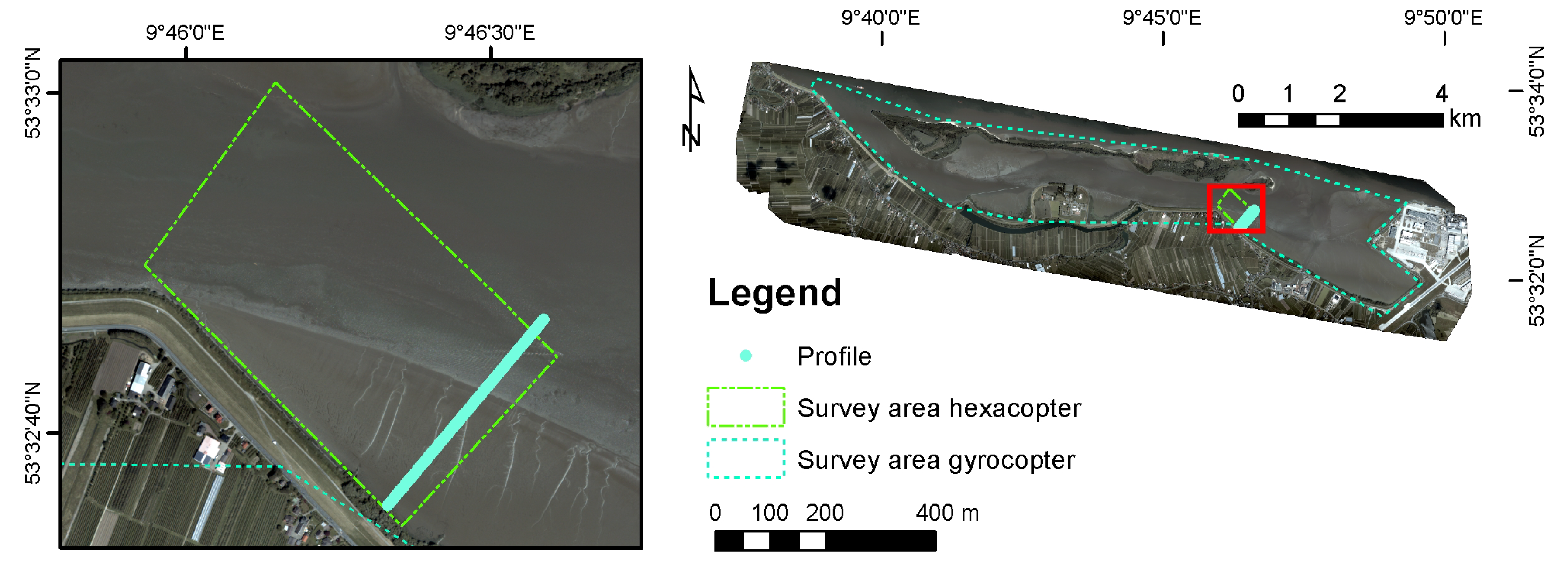
Research Area

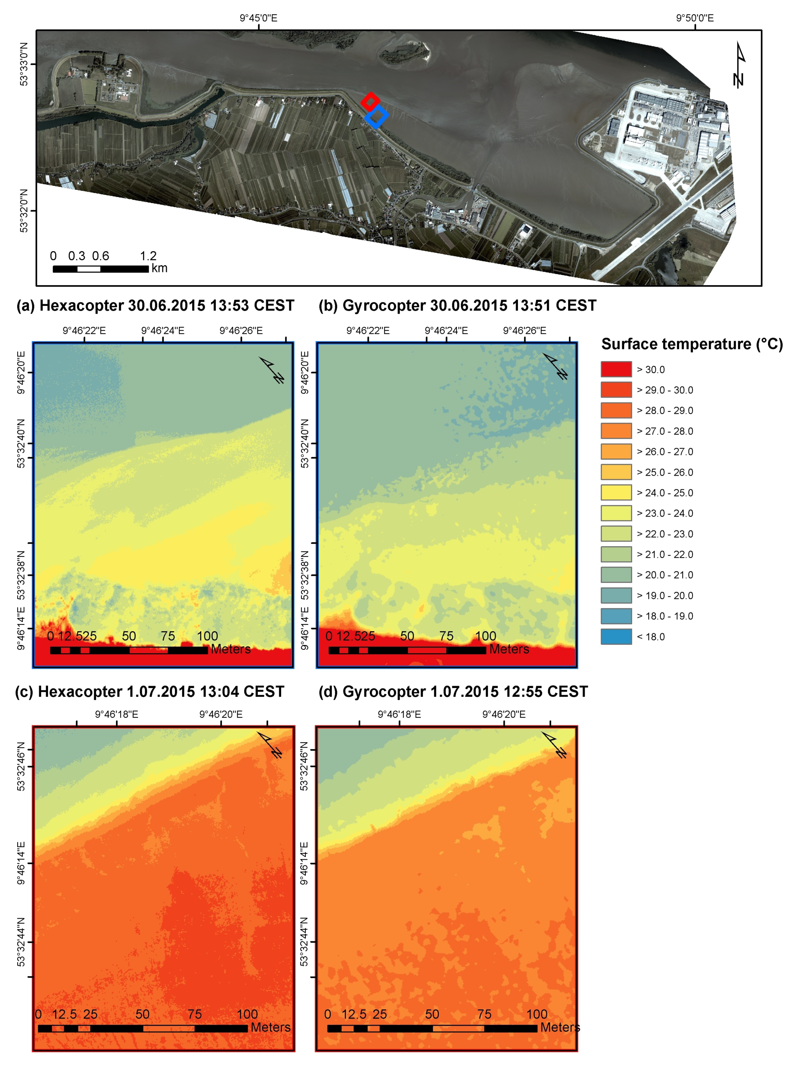
The research area is the Hahnöfer Nebenelbe, a side channel of the Elbe estuary downstream of Hamburg (see Figure 1). It is a mesotidal estuary [25], where the tides are responsible for regularly changing water levels, flow, and mixing processes [26]. The side channel is oriented along the flow direction from east to west, parallel to the main channel. It is separated from the main channel by two narrow islands (downstream Hanskalbsand and upstream Neßsand) in the North and confined by the Altes Land dikes, an area of reclaimed marshland in the South. Furthermore, located in the research area are the smaller island Schweinesand, the former and now reclaimed island Hahnöfer Sand and several shallow intertidal mudflats that are periodically flooded during the tide. The large water body in the east is called Mühlenberger Loch and is defined as a bird sanctuary and protected area, part of the Natura 2000 network.

During the diurnal flooding of the Hahnöfer Nebenelbe, the water enters downstream of Hanskalbsand and upstream of Neßsand and the water masses meet South of Neßsand. The water also gradually overflows the tidal mudflats next to the islands and the dike. Due to the mixing point location and the potential survey of a channel and tidal mudflats simultaneously, the survey area of the hexacopter was planned for this part of the side channel (dashed green line in Figure 1). Additional considerations included a suitable landing place and a view of the flight area unobstructed by trees from the dike. For the gyrocopter, the whole Hahnöfer Nebenelbe and a part of the main Elbe channel were chosen as the survey area (dotted blue line in Figure 1).

2. Methodology

2.1. Data Acquisition

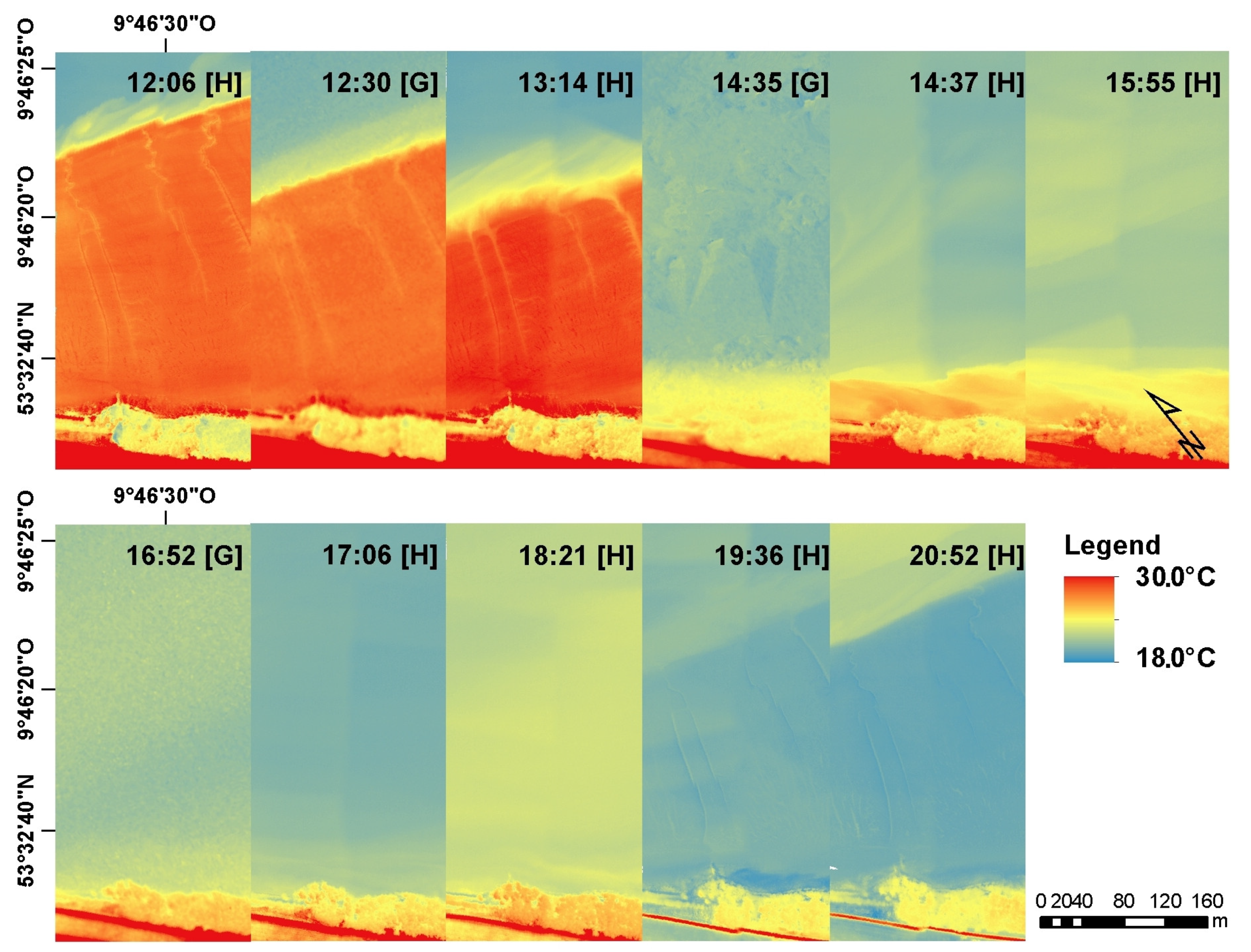
Water surface temperature should be recorded when the temperature contrasts are high to facilitate the identification of temperature patterns and underlying transport processes. This is the case during the summer, when high solar insolation coincides with low tide shortly before noon, the tide then floods the heated intertidal mudflats with colder water from the main stream. When the tide is falling again, the heated water from the mudflats drains into the channels. The aerial survey was conducted on 30th June and 1st July 2015. The flight days were selected based on the predicted water levels and weather conditions. The weather on the two acquisition days was sunny, with few clouds and average wind speeds of 3 ms${}^{-1}$ and 4 ms${}^{-1}$, respectively.

A combined aerial survey with a piloted gyrocopter and an unmanned hexacopter (6-rotor UAV), as well as in situ measurements, were conducted with the aim to acquire spatially distributed thermal infrared (TIR) data by the Application Center for Multimodal and Airborne Sensors (AMLS), a contracted engineering company, and the Federal Institute of Hydrology (BfG), Germany. The use of gyrocopter and hexacopter permitted only a limited payload and available energy for the imaging systems but allowed to perform multiple flights. The data acquisition included several flights by two aerial systems, seven by the gyrocopter, and 16 by the hexacopter (for specifications see

Table 1. Specifications of the TIR sensors and image acquisition. The overlap is measured along-track and between flight lines.

Platform	Gyrocopter	Hexacopter
Altitude	1300 m	100 m
Sensor	Pearleye P-030 LWIR	Optris PI450
Weight	790 g	320 g
Field of view (FOV)	25.1${}^{\circ }$ × 19.6${}^{\circ }$	31${}^{\circ }$ × 23${}^{\circ }$
Spectral range	8–14 $\mathsf{\mu }$m	7.5–13 $\mathsf{\mu }$m
TIR resolution	640 × 480 pixel	382 × 288 pixel
Spatial resolution	1.8 m	0.35 m
Thermal sensitivity	≤80 mK	40 mK
Measurement accuracy		$\pm 2{}^{\circ }$C or $\pm 2$%
Image frequency	up to 24 fps	80 Hz
Overlap	80%/30%	70–80%/40–50%

). The flights were timed during the tidal phases to catch all essential states of temperature patterns (see Figure 2). Additionally, in situ measurements of Elbe water quality and temperature, water levels, weather data, and calibration/reference measurements for the TIR cameras with additional water temperature loggers and a TIR thermometer.

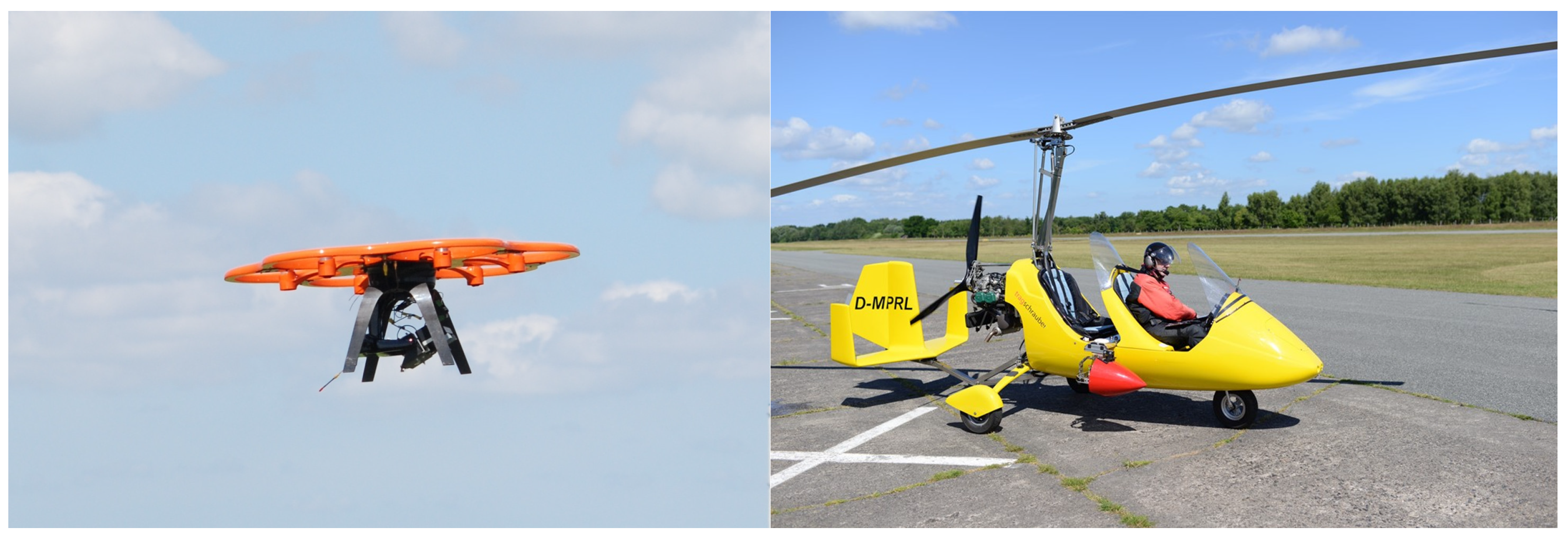
2.1.1. Gyrocopter

A gyrocopter, also known as an autogyro, acquired data of the whole Hahnöfer Nebenelbe (24 km${}^2$) by overlapping images along four parallel flight paths in a west–east direction. Mounted on the gyrocopter was a Pearleye P-030 LWIR from Allied Vision Technologies, measuring in the 8–14 $\mathsf{\mu }$m wavelength region with a sensitivity of 0.08 K (see Figure 3).The manufacturer did not publish a specification of the absolute measurement accuracy. The microbolometer sensor is temperature stabilized by a thermoelectric cooler (TEC), i.e., a Peltier element. After Tempelhahn et al. [27], the constant temperature prevents “the sensor parameters’ offset voltage and responsivity to change according to the ambient temperature”. This reduces temperature variations during the flight and, therefore, the noise in the final images. The camera’s viewing angel is up to 30.5${}^{\circ }$, and at a flight altitude of 1300 m above ground, the spatial resolution of the TIR images was 1.8 m and the RGB resolution reached 0.6 m. The resulting mean geolocation error of the referenced TIR images was 1.96 m.

Post-processing of the temperature images with the “structure from motion” (SfM) algorithm [28] was possible due to the dual-camera setup PanTIR built by AMLS: it combines the Pearleye thermal infrared camera with a high-resolution camera in the visible wavelength region [29]. The high-resolution images are used as a reference for the thermal images and improve the mosaic stitching and geo-referencing, which was previously difficult due to the relatively low water temperature contrast in the thermal images. The geo-referencing was based on the GPS positions of the cameras during acquisition, with additional manual referencing based on ground control points. The duration of the acquisition flights, the distance to the airfield used, and the proximity to two other airports, Hamburg Airport, and Hamburg Finkenwerder Airport, allowed for four planned flights per day. Due to flight restrictions, one flight had to be canceled on the second day.

2.1.2. Hexacopter

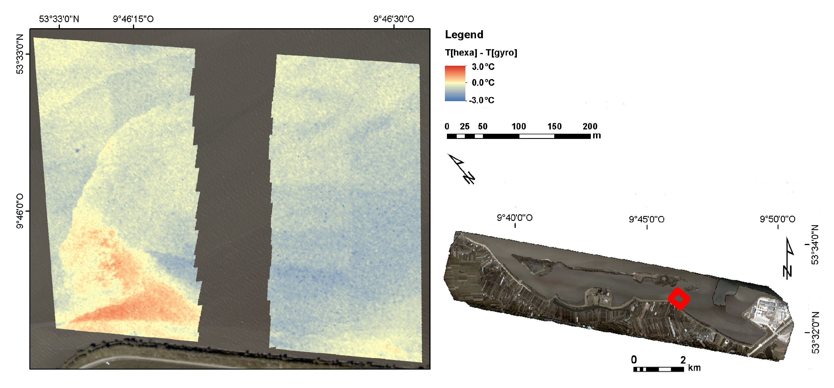
Additionally to the gyrocopter survey, a hexacopter (6-rotor UAV) acquired multispectral and thermal data (see Figure 3). Due to flight altitude and range of the hexacopter, it covered a far smaller survey area at a higher spatial and temporal resolution than the gyrocopter (0.25 km${}^2$). A section of intertidal mudflats and a fairway in front of the dike south of the Hahnöfer Nebenelbe was chosen for a detailed survey, where the temperature differences are especially pronounced during the tidal cycle. Only one continuous measurement station was located inside the survey area, but the area boundaries could not be modified due to the necessary accessibility and line of sight. The hexacopter pilot operated the UAV based on a dike at the southern river bank. The flight altitude was limited to 100 m due to the bird sanctuary next to the survey area.

To cover the hexacopter survey area, it took approximately one hour, eight flight lines, and battery changes every two flight lines. The image acquisition frequency was increased on the second day to allow for the selection and dismissal of images taken with an extreme camera tilt due to wind gusts. The thermal camera on the hexacopter was an Optris PI450 (uncooled microbolometer) that acquired observed surface temperatures in the wavelength region of 7.5–13 $\mathsf{\mu }$m with a sensitivity of 0.08 K, an accuracy of $\pm 2{}^{\circ }$C/$\pm 2\%$, and a pixel resolution of 382 × 288 pixels. The viewing angle of the camera is up to 26.5${}^{\circ }$. The hexacopter was able to cover the survey area eight times per day on both days. The hexacopter images were then referenced individually based on the system’s differential global positioning system (DGPS) measurements and position of the camera gimbal. The resulting mean geolocation error of the referenced TIR images was 3.31 m.

2.1.3. In Situ Measurements

Besides the thermal images acquired by gyrocopter and hexacopter, several other data sets were used to evaluate and correct the aerial data sets. Weather data was collected from the meteorological weather station Fuhlsbüttel, Hamburg, operated by the German Meteorological Office (Deutscher Wetterdienst, DWD) and provided online at the Climate Data Center [30]. Several weather parameters were also collected onboard the gyrocopter, operated by AMLS. The water levels, necessary to determine the tidal cycle in the research area, were measured at several water gauge stations, operated by the Federal Waterway Administration (Wasser- und Schifffahrtsverwaltung, WSV).

In situ measurements of the water body temperature, $T_w$ from three continuous multi-parameter buoy measurements were provided by the BfG. Additionally, four temperature data loggers (Driesen + Kern underwater temperature data logger) were deployed by BfG and WSV in summer 2015 and attached to lateral marks near the hexacopter survey area. The number of measurement locations is small due to the limited accessibility of the mudflats and dense vegetation areas at the shore. While the $T_w$ measurements were used to evaluate the aerial data directly, calibration tests were setup for both the gyrocopter and hexacopter TIR camera: before each flight, the TIR cameras captured the image of a water tub in which a temperature data logger was immersed. At the hexacopter launch site, a thermal infrared thermometer (IR120 by Campbell Scientific) was added to the setup. The absolute accuracy of in situ measurements of the water body temperature $T_w$ was between 0.15 and 0.2 ${}^{\circ }$C.

2.2. Sources of Error and Uncertainty

When evaluating water surface temperatures measured by airborne thermal sensors, there are several sources for error and uncertainty to consider. The error described the difference between the idealized “true value” and the measured value, which is unknowable, while the uncertainty is characterized by the variation of the values that are in all probability describing the measured variable [31]. These include the accuracy and precision of the sensor [32,33,34], sensor noise, and vignetting due to characteristics of the sensor and viewing geometry [35,36]. The thermal cameras used in this survey have not the radiometric and focal plane array calibration and stability that cryogenically cooled cameras offer [12] and require additional calibration steps and processes (e.g., [32,33,34]). Furthermore, the temperature signal travels through the atmosphere between the sensor and observed surface and is affected by the transmissivity, up and down welling radiance [11,12,35]. At the water surface, we have to consider that the TIR sensor cannot observe the actual top water surface, but the radiance emitted from the “radiometric skin depth” [37], which is the top 50–100 $\mathsf{\mu }$m [38]. The observed surface temperature is depending on the emissivity/reflectivity [12,35,36,39,40] as well as on thermal boundary layer effects and possibly stratification below the water surface [11,12,41,42,43,44,45]. Environmental effects may also include scattering from the near-bank environment and the adjacency effect [11,36]. Shadows have been cited by other authors to influence the radiant temperature of the water surface [11,12], but were not visible in the acquired thermal imagery. With regards to methodology, mixed pixels, the spatial uncertainty of comparison pixels, and the temporal variability of in situ measurements (sampling uncertainty) come into play during the evaluation and assessment of the results [12,38].

Random observational errors tend to cancel out when large numbers are averaged together due to the independence of the individual errors, but systematic observational errors have to be analysed and examined closely [31]. In the next subsections, these uncertainties and error sources are discussed based on the results from other authors and our assessment of their relevance in this survey, before correction steps are proposed.

2.3. Evaluation of the Datasets and Validation of the Correction Steps

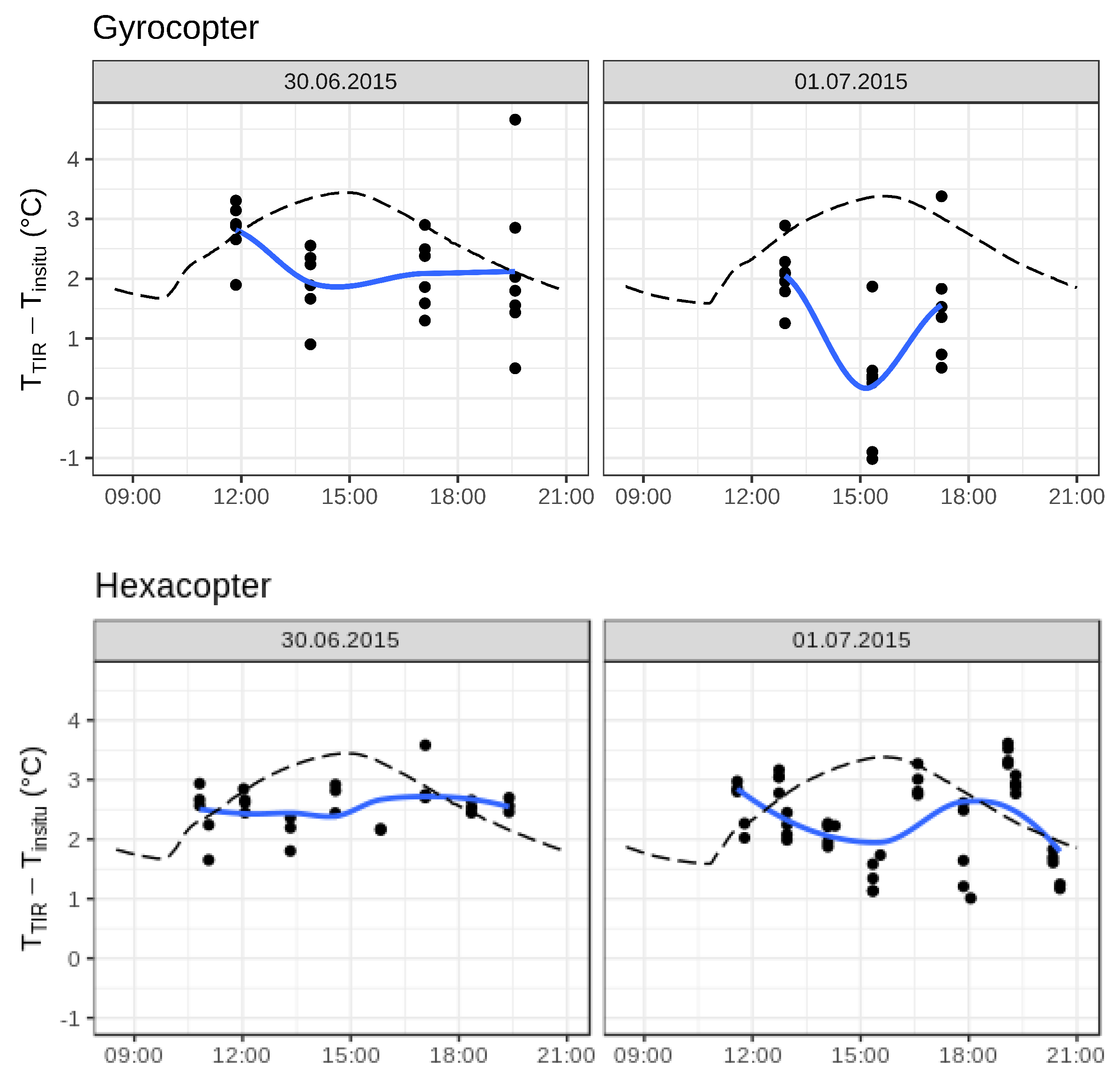
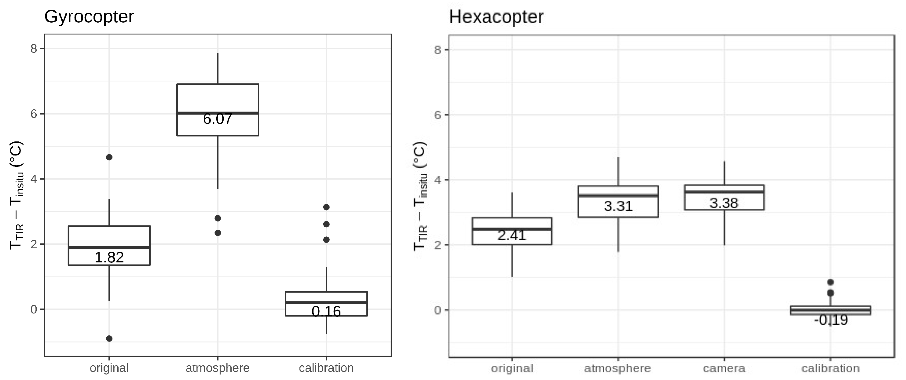
To evaluate the acquired data sets and to validate subsequent processing and correction steps, the temperature value from the individual hexacopter images and large gyrocopter mosaics was extracted automatically at the known coordinates of measurement locations and compared to in situ measurements of the water temperature as a reference. Eight measurement stations were located in the gyrocopter survey area and, due to its smaller size, one in the hexacopter survey area. The extracted differences were then grouped by flights (see Figure 4).

The automated extraction of single-pixel values can also lead to the extraction of pixels that are not necessarily representative of the water temperature at the measurement location due to mixed pixels of water and actual non-water objects, water temperature boundaries or georeferencing error [12,38]. For the hexacopter TIR dataset, different extraction methods were tested: (i) the extraction and averaging of a 3 × 3 pixel window instead of a single-pixel and (ii) the manual extraction of a water pixel closest to the visible measurement location instead of the automatic extraction at the provided geographic coordinates. The resulting change of $T_{TIR}$ was (i) −0.06 ± 0.32 ${}^{\circ }$C and (ii) 0.01 ± 0.22 ${}^{\circ }$C. The different methods had a larger effect on the variability of the extracted temperatures and less on the mean value. The evaluation of the datasets was consequently based on the automated extraction of single pixels, as the test methods required significantly more computing time or manual labour without a significant effect on the evaluation results. However, special attention was given to the possible occurence of outliers.

2.4. Emissivity Correction

For the emissivity of water, a constant value is often assumed in a range between 0.96 and 0.99, as it changes very little compared to emissivities of land cover surfaces. However, the emissivity of water depends on the composition of the water (e.g., sea vs. fresh water, sediment amount, dissolved minerals) [36,40], wavelength, observation angle, and surface roughness [36]. Small observation angles up to 30${}^{\circ }$ lead to a small decrease in emissivity and temperature, in most cases negligible [36], but only 1% uncertainty of the emissivity may lead to a 0.4 K error on the surface temperature retrieval under standard conditions [35]. As the individual hexacopter images featured strong vignetting with decreasing temperature values towards the edges, this potential error source was investigated.

Masuda et al. [46] developed an emissivity model applying the Fresnel relationship between incident radiant power and the reflected and refracted power at the boundary between different dielectric media. It suitably represents the actual emissivity values for viewing angles up to 40${}^{\circ }$ (see also [39]), and it has been widely used [47,48]. The emissivity values are calculated based on optical constants, viewing angles, and local wind speeds (for modelled emissivity values during the survey, see Figure 5). In this study, the observation angle was used as incidence angle as no large waves were observed during the data acquisition, and the water surface was assumed to be level.

Other phenomenons that influence the emissivity are foam (from either natural or anthropogenic origin, lower emissivity and observed surface temperatures) and anomalies due to boat plumes that change the water surface roughness [12]. Simultaneously acquired RGB images can help identify these effects. As they occurred only occasionally in very small areas in the acquired images and did not affect the $T_{TIR}$ at the locations of the in situ measurements, they were not corrected.

2.5. Atmospheric Correction

The temperature signal of the observed surface travels through the atmosphere before it is received by the sensor and is affected by several factors: the transmissivity, up and downwards radiance [11,35,49]. The influence of the atmosphere ist mainly depending on the water content of the atmosphere, which is notoriously difficult to assess and for standard atmospheric water vapour content an error for $T_s$ of 0.7 K is to be expected [35]. Thermal scattering from the near-bank environment was also considered, but is only relevant under low observation angles [38] and was expected to be small compared to $T_{water}$.

The measured $T_{TIR}$ were converted to radiance $L_{meas}$ with Planck’s radiation law and corrected in a single-band-approach [35,50,51] based on the constant or calculated emissivity $\epsilon$ (see Section 2.4) and atmospheric parameters upwelling radiance $L_a^{up}$, downwelling radiance $L_a^{down}$, and transmissivity $\tau$ calculated with the radiative transfer model MODTRAN5.3.2. [52].

$$L_{meas}=(\epsilon L_{surface}+(1-\epsilon )L_a^{down})\tau +L_a^{up}.$$

(1)

MODTRAN5.3.2. requires input parameters such as aerosol type, atmosphere type or profile, weather data, sensor information, ground elevation and sensor altitude. The influence of the input parameters on the influence of the atmospheric correction was evaluated by a sensitivity test that was conducted for the $T_{TIR}$ mosaic from the first gyrocopter flight with different MODTRAN input parameter sets and compared with $T_w$ measurements from in situ measurement locations (see Fricke et al. [53] for more detailed results). As it turned out, only a small effect on the corrected surface temperatures had the inclusion of different weather station data ($\pm 0.1{}^{\circ }$C), the chosen aerosol type ($\pm 0.2{}^{\circ }$C), and the integrated calculation of the transmissivity ($\pm 0.2{}^{\circ }$C). The effect of changes in altitude was $\pm 0.15{}^{\circ }$C/100 m. On the other hand, the selection of the model atmosphere had a more significant effect of up to 0.5 ${}^{\circ }$C, and changes in the sensor bandwidth have a substantial effect of several degrees Celsius. The transmissivity of the atmosphere decreases rapidly below 8 $\mathsf{\mu }$m and above 14 $\mathsf{\mu }$m and therefore, an incorrectly chosen, too large bandwidth can cause an overestimation of the corrected $T_{TIR}$ (see also [54]). Based on the sensitivity test, the following input parameters were decided for the radiative transfer model: the local climate station data, the U.S. standard atmospheric profile adapted to the weather information by the gyrocopter at flight altitude, a maritime aerosol type, and the flight altitude above ground as recorded by the gyrocopter and hexacopter. The transmissivity was integrated over the wavelength, and the bandwidth was the full width at half maximum from the manufacturer specification as suggested by Barsi et al. [54], which was for both cameras close to 8–13 $\mathsf{\mu }$m.

It was also considered to calculate the atmospheric parameters depending on the viewing angle, mainly the transmissivity [35]. In this case, it changed the results only marginally (<0.1 ${}^{\circ }$C, [53]) but required disproportionally high computing time, and therefore was omitted for this correction step. In contrast, the inclusion of the angle and wind dependent emissivity was easily executed and therefore incorporated in the atmospheric correction (see Equation (1)).

2.6. Camera Flat Field Correction

A vignette effect and decreasing temperatures towards the image borders were observed in the individual images from both hexacopter and gyrocopter. Possible causes include a sensor error, the lens geometry, and angle-dependent emissivity and atmospheric effects. Nugent et al. [33] state that microbolometer detectors without “a thermoelectric cooler to stabilize the focal plane array temperature, the calibration must be updated nearly continuously”.

The gyrocopter camera has a calibration process that uses a shutter to reduce the vignetting and the variability across the individual TIR images. Laboratory measurements have shown that when viewing a black body with a uniform temperature, the shutter calibration can reduce the standard deviation across the thermal image from 1.4 ${}^{\circ }$C to 0.1 ${}^{\circ }$C. Together with the high overlap of the individual images acquired by the gyrocopter, the individual images could be aligned, and the mosaics could be created without necessarily correcting the remaining vignetting.

The overlap of the individual images acquired by the hexacopter proved to be insufficient compared to the stronger temperature gradient towards the image border. Therefore, the vignette was also visible in the mosaics. A laboratory flat field calibration as described by [32] was substituted with an image-based flat field correction during post-processing. This camera correction is based on a per-pixel correction value look-up table (LUT), which is determined by the offset of each pixel compared to the value of the center pixel in the acquired images. Image based LUTs are more accurate and more straightforward to calculate for images acquired in the visible wavelength range compared to optical modeling approaches [55]. The usage of a large number of calibration images also averages out the random noise component in the data [55].

For this case, images with a standard deviation of temperature values lower than 0.25 ${}^{\circ }$C were selected as calibration images, as they were assumed to represent a water surface with a nearly uniform temperature where the deviations stem mainly from sensor noise. The correction value $\Delta {\overline{T}}_i^{cal}$ for every pixel i was calculated as the mean temperature difference in all selected calibration images between the image’s center pixel ${\overline{T}}_{center}^{cal}$ and the selected pixel ${\overline{T}}_i^{cal}$. The calibration value $\Delta {\overline{T}}_i^{cal}$ was then subtracted from the original pixel value $T_i$ to calculate the corrected pixel value $T_i^{corr}$.

$$\Delta {\overline{T}}_i^{cal}={\overline{T}}_{center}^{cal}-{\overline{T}}_i^{cal}$$

(2)

$$T_i^{corr}=T_i-\Delta {\overline{T}}_i^{cal}$$

(3)

Additionally to the precision and relative accuracy of measurements across the camera sensor, the accuracy of a sensor and stability of the absolute calibration is essential [35,36]. Especially uncooled TIR sensors tend to be affected by the ambient air temperature and, therefore, show a low absolute accuracy when used in the field [32,33,34]. These issues are discussed in Section 2.8. Furthermore, the sensor response function was not known for both cameras. The sensor response function describing the bandpass and FWHM effects of the sensor may alter the results when not considered and can lead to a 0.15 K difference for a surface temperature of 300 K in the TIR wavelength region [35]. Lens distortions may also affect the TIR images, but a correction was not applied as the expected improvement is relatively small [55,56].

2.7. Temperature Stratification and Skin Effect

Another source of error for the remote sensing of water temperatures is the possible difference between the water surface and water layers below, from skin to subskin and water body temperature [11,18,39,44]. Different processes can lead to a non-linear vertical temperature gradient: evaporation and heat exchange produce a cooler surface and skin water temperature (“skin effect”), while diurnal heating due to solar radiance would warm the skin and subskin water more than the water body layer and lead to thermal stratification below the surface. For an indepth description of the mechanisms, refer to [43].

TIR sensors measure the radiation from only the upper submillimeter-thick skin of the water body [39,41], where the skin layer is almost always present [57,58]. Based on the model developed for the skin effect in SST measurements at nighttime and daytime during strong wind conditions [44] and the average wind speed of 3 and 4 ms${}^{-1}$ for the survey days, the difference between skin and the bulk temperature was expected to be about −0.2 ${}^{\circ }$C. This is similar in magnitude to the skin effect for lake surface temperatures (LST) in a moderate climate, which was 0.1–0.2 K for 3 to 4 ms${}^{-1}$ wind speed in [59] and 0.11–0.46 ${}^{\circ }$C in [42], depending on the daytime/nighttime and mixing due to wind, with a higher standard deviation of the daytime skin effect due to variable stratification. The skin temperature is also strongly correlated to the air temperature [60]. Shade from the bank vegetation covered only a very small part of the images and had no visible effect on the TIR temperatures [38].

If there is no thermal stratification, e.g., due to wind turbulence, sub-skin water surface temperatures can be close to in situ measurements of the bulk water temperature [37]. However, under clear and calm conditions and subsequently strong insolation, a warm layer can develop below the surface (sub-skin) compared to the cooler bulk water temperature and form a thermocline [41]. These temperature variations within the top water layers can lead to significant errors in remotely sensed water temperatures compared to in situ measurements.

2.8. In Situ Calibration and Validation

Generally, an absolute temperature calibration of TIR sensors can be achieved by periodically viewing one or more external blackbody sources, either in a laboratory calibration before flight, or cooled black body calibration in flight. Cost-effective and lightweight thermal cameras or sensors typically forgo cryogenically cooled black body calibration in flight due to weight and space constraints. This can pose a significant problem for absolute measurements as the sensor responds to changing ambient temperatures. It is recommended for uncooled bolometers to let the camera acclimate to the ambient temperature first [12], even for several minutes [34].

Reference measurements at ground level with the gyrocopter TIR camera were not usable for calibration as the flight altitude of 1300 m lead to a decrease in ambient air temperature of about −16 ${}^{\circ }$C compared to the ambient ground temperature. Laboratory measurements with the gyrocopter camera simulating the ambient conditions during the survey flights showed a 5.7 ± 0.15 ${}^{\circ }$C temperature difference due to changing sensor performance with changing ambient and camera temperature. Laboratory measurements with the sensor carried by the hexacopter were not feasible, so the only opportunity to calibrate the radiometric temperature measured by the TIR sensors would be based on the in situ measurements. This means that the resulting calibrated datasets would represent the kinetic water body temperatures.

A nearly linear relationship between $T_{TIR}$ and $T_{insitu}$ measured by temperature loggers has been reported [38]. It has been the traditional approach for calculating SST based on the regression between satellite radiances against ship data/buoy measurements to produce SST consistent with the traditional bulk SST observations [57,61,62]. The calibration should be conducted after atmospheric correction, as the relationship between water surface temperature to brightness temperatures and atmospheric state is supposedly non-linear [62] and should be corrected first. Assuming that the previous corrections reduced or eliminated the variable effects on individual images or parts of the mosaic, an in situ calibration method for the whole flight mosaics was developed (see also [18]).

To fully utilize the number of in situ measurements available, cross-validation with the leave-one-out method was chosen for the simultaneous calibration and validation of the mosaics. Given n data pairs in the data set, this method uses $n-1$ pairs as a training set to fit a model explaining the relationship between the data points, and the remaining pair is then used as a test set to evaluate the fit of the model and to perform the validation. This procedure is repeated until all data pairs have been used as a test set, and the mean error can be calculated for the chosen model. Several models and data set sizes were tested on the available data pairs, but in the end, linear regression with a slope equal to one, i.e., a simple bias correction, was chosen to correct each flight (mosaic) separately.

$$T_{insitu}=a_0+a_1\ast T_{TIR},a_1=1$$

(4)

Due to the high variability of the difference $\Delta T_{TIR}$ between $T_{TIR}$ and $T_{insitu}$ and occurrence of outliers, models based on polynomial equations of a higher degree tended to overfit and suggested improbable relationships between $T_{TIR}$ and $T_{insitu}$. Similarly, the slope was fixed at one to reduce the effect outliers could have on the individual linear models which were repeatedly calculated on a small number of data pairs for each flight and produced implausible high positive and negative slope values. Models fitted to data pairs from individual flights produced better results than models fitted to all data pairs or only from one day as average $\Delta T_{TIR}$ was varying throughout the survey days (see Figure 4). Additionally, in the gyrocopter datasets $T_{insitu,g}$ values outside the interval of $\mu \pm z_p\sigma$ with the quantile $z_p$ = 1.645 (90% tolerance interval) were omitted as outliers as $\Delta T_{TIR,g}$ showed a higher variance, to prevent the fitting of statistically sound, but implausible models. This step was omitted for the hexacopter cross-calibration as there were not enough data pairs available for each flight.

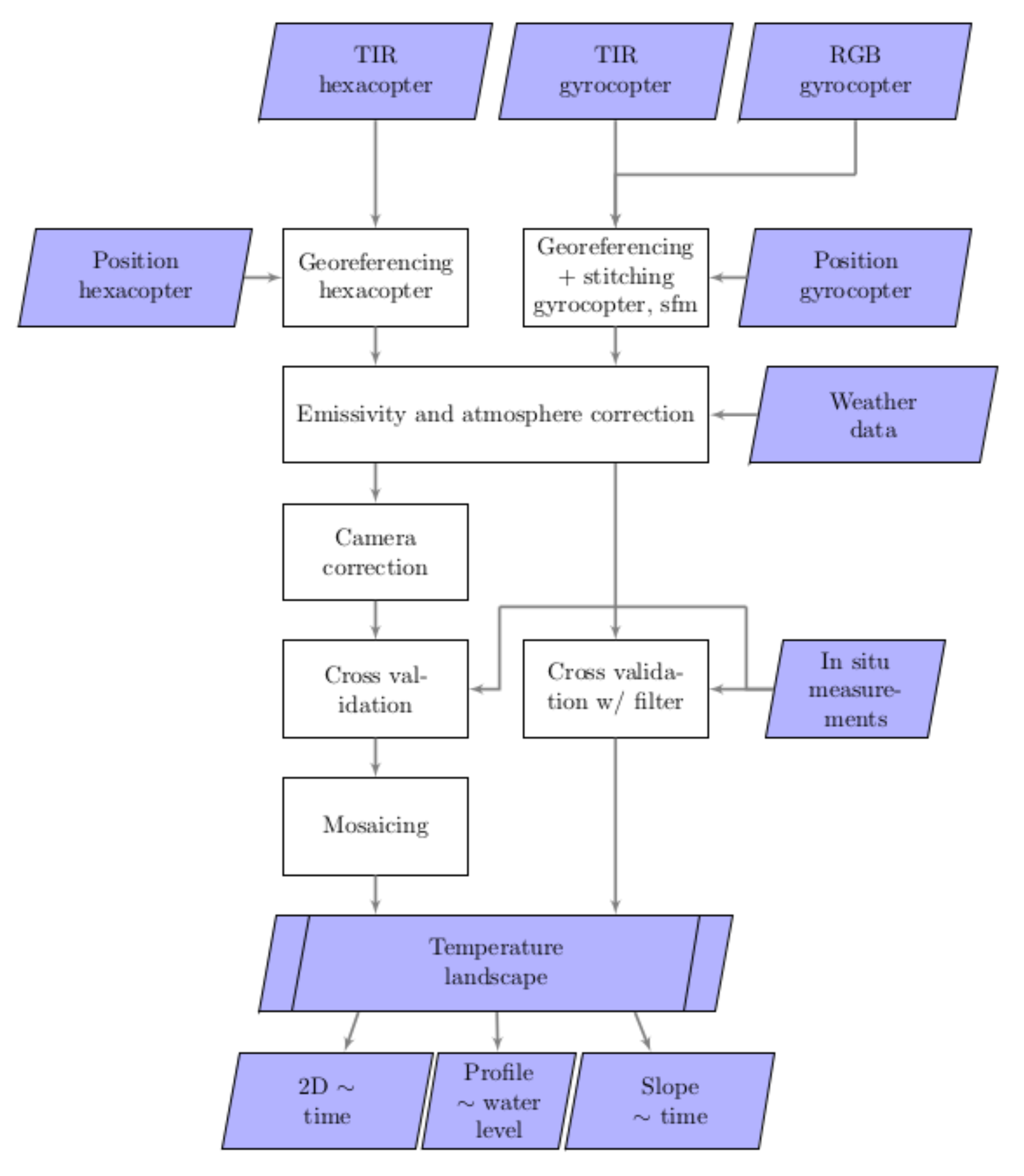
2.9. Processing and Workflow

A schematic overview of the correction steps can be found in Figure 6. The Python programming language was used (Python Software Foundation, https://www.python.org/ (accessed on 6 April 2021)) for calculating the individual correction steps. From there on, mosaics based on the individual hexacopter images were created with the Erdas Imagine 2015 Mosaic Pro Tool (Hexagon Geospatial, https://www.hexagongeospatial.com/products/power-portfolio/erdas-imagine (accessed on 6 April 2021)). The seamlines were based on the distance to nadir to increase the mosaicking process’s reproducibility and comparability, and calculated with feathering over 5 m at the seamlines.

As it was not necessary to correct angle-dependent effects on the gyrocopter data due to the larger overlap, the detailed emissivity calculation and correction was only applied to the hexacopter images.

3. Results

3.1. Evaluation of the Original Data Sets

For both camera systems, the initial absolute accuracy was expected to be low, while the relative accuracy (precision) should be high (Table 1). When comparing the uncorrected water temperature values acquired by the TIR cameras ($T_{TIR}$) with the in situ measurements $T_{insitu}$, both remote sensing systems tend to overestimate the water body temperature. For the gyrocopter, the mean difference between $T_{TIR,g}$ and $T_{insitu}$ is 1.82 ${}^{\circ }$C, with a standard deviation of 1.10 ${}^{\circ }$C. The comparison of the hexacopter images shows a mean difference $\Delta T_{TIR,h}$ of 2.41 ± 0.63 ${}^{\circ }$C. The temperature difference is very variable across both measurement location and acquisition time and higher than the supposed sensitivity (see Table 1). The variability of the gyrocopter dataset was expected to be smaller due to aggregation in the slightly larger pixels [38] at the in situ measurement locations, but the effect of the very different measurement stations was larger.

Additionally, the individual TIR images exhibit a significant vignette effect with decreasing temperature values towards the hexacopter’s TIR image borders (up to 0.6 ${}^{\circ }$C). An even significant decrease was observed in the individual gyrocopter images (up to 4.5 ${}^{\circ }$C), but fortunately cut off during the mosaicking (see overlap in Figure 1).

3.2. Emissivity Correction

The angle-dependent emissivity correction based on Masuda et al. [46] has been calculated for the individual gyrocopter and hexacopter TIR images, which then were compared to in situ measurements [53]. The correction for emissivity ($\epsilon =0.99$) increased the overall $T_{TIR}$ in the datasets by about 0.6 ${}^{\circ }$C. On the border of the TIR images, calculating the emissivity, including the maximum viewing angle and the wind speed could lead to an additional increase of up to 0.15 ${}^{\circ }$C. However, this correction step has only a minimal effect on the average absolute difference when comparing $T_{TIR}$ and $T_{insitu}$ as only the outermost pixels of the individual images are affected by this correction. The effect of including the viewing angle in the emissivity correction was on average 0.1–0.2 ${}^{\circ }$C, including the surface roughness represented by the wind speed (3 ms${}^{-1}$ and 4 ms${}^{-1}$ on both survey days, respectively) was ±0.1 ${}^{\circ }$C [53]. The angle-dependent emissivity correction does reduce the variability of the TIR temperatures and improves the hexacopter mosaics, as it calculates the emissivity depending on their viewing angle and therefore reduces the vignette effect (see Figure 5).

3.3. Atmospheric Correction

For both the hexacopter images and the gyrocopter mosaics, $T_{TIR}$ was corrected according to Equation (1) for emissivity and atmospheric effects. The typical atmosphere in this region and season reduces the radiance temperatures acquired by the sensor: the atmosphere is colder than the earth’s surface, absorbs radiance and reduces the transmitted $T_{meas}$ at the sensor. Thus, atmospheric correction leads to higher $T_{TIR}$ (see Figure 7). The atmospheric correction is not linearly related to the altitude as the atmosphere is denser at lower altitudes. Hence the atmospheric correction is relevant for both sensor platforms despite the low flight altitude of the hexacopter. The atmospheric correction effect is, on average, ∼1.1 ${}^{\circ }$C for the hexacopter ($\Delta T_{TIR,h}$ = 3.31 ± 0.69 ${}^{\circ }$C after the correction step) and ∼4.25 ${}^{\circ }$C for the gyrocopter $T_{TIR,g}$ ($\Delta T_{TIR,g}$ = 6.07 ± 1.42 ${}^{\circ }$C after the correction step) when compared with $T_{insitu}$. The effect on the $T_{TIR,g}$ is slightly larger as the atmospheric layer between the gyrocopter and the water surface is greater.

3.4. Camera Flat Field Correction

When comparing the mosaics of hexacopter images before and after the camera correction in Figure 8, they show that the vignette effect has been improved in the mosaic, although absolute differences between the individual images still prevail. When comparing the $T_{TIR,h}$ to $T_{insitu}$ measurements (Figure 7), the difference $\Delta T_{TIR,h}$ = 3.38 ± 0.66 ${}^{\circ }$C, has increased on average as the temperatures at the borders became slightly higher, but the variance has slightly decreased.

3.5. Temperature Stratification and Skin Effect

Concerning potential diurnal heating and thermal stratification at the measurement locations used in this survey, in situ temperature logger measurements at several heights (varying water depth depending on the tide as they were fixed on metal poles 10 cm, 30 cm, and 50 cm above ground) in 2014 showed minimal (0.1 ${}^{\circ }$C) or no thermal stratification in the water bodies over the wadden flats. As the survey has been conducted in a tidal area, strong currents and mixing processes can be expected and may prevent developing a temperature gradient. The water temperatures measured by the temperature loggers over the wadden flats tend to differ from the bulk water temperatures at the permanent in situ measurement stations [53], which, after analysing in situ measurements and acquired TIR temperature patterns, the authors conclude to be due to lateral temperature differences based on the different locations (wadden flats vs. channel).

After atmospheric and camera flat field correction, the remaining difference between $T_{TIR}$ and $T_{insitu}$ can be explained by two error sources: a camera (calibration) error and the skin effect (see Section 2.2). During the survey reference measurements with mobile calibration targets (i.e., water-filled boxes with a temperature data logger) have been conducted before each flight of the TIR sensors but led to inconclusive results about the data bias related to calibration error and skin effect (results in [53]: mean difference during the calibration between $T_{TIR,g}$ and $T_{logger}$ was −1.63 ${}^{\circ }$C, and between $T_{TIR,h}$ and $T_{logger}$ was 1.36 ${}^{\circ }$C. If we regard the mean temperature differences after emissivity and atmospheric correction during the flight, the bias of the hexacopter data becomes slightly larger during the flights, while the gyrocopter bias changes significantly and overestimates $T_{insitu}$ during flight.

Reference measurements of the calibration target’s water surface temperature with an IR thermometer (CampbellScientific IR120) underestimated the water temperatures (−2.12 ${}^{\circ }$C), indicating a systematic error and could not be used to quantify the skin effect during the survey [53]. In an attempt to quantify at least the camera sensor offset due to ambient temperature changes from the ground to flight altitude, these were simulated in the laboratory with the gyrocopter camera (PearlEye P-030) in a climate chamber (see Section 2.8). They show that a difference of $\sim +$5.7 ${}^{\circ }$C can be explained by the TIR sensor reacting to ambient temperature changes. If we assume the observed bias is transferable to the survey, this leads to an estimated skin effect of 0.37 ${}^{\circ }$C. The magnitude is well within the possible range [42,44,59], considering the uncertainties in its derivation.

3.6. In Situ Calibration and Validation

After emissivity and atmospheric correction, the mean difference $\Delta T_{TIR,g}$ between $T_{TIR,g}$ and $T_{insitu}$ was 6.07 ± 1.42 ${}^{\circ }$C and varied from flight to flight (3.82 ${}^{\circ }$C to 7.53 ${}^{\circ }$C). The mean difference $\Delta T_{TIR,h}$ between $T_{TIR,h}$ and $T_{insitu}$ after atmospheric and camera correction was 3.38 ± 0.66 ${}^{\circ }$C with less variability between flights (2.07 ${}^{\circ }$C to 4.13 ${}^{\circ }$C). These remaining differences were attributed to the effect of varying ambient conditions (air temperature, wind speed, humidity) on the TIR camera sensor, the skin effect, which is present even in well-mixed water bodies [57,58], or adjacency effect from the surrounding environment [11,38]. All three were difficult, if not impossible, to determine accurately during the field surveys. As discussed in Section 2.8, a calibration based on in situ measurements was applied. With the calibration, according to the cross-validation, $\Delta T_{TIR,g}$ could be reduced to 0.16 ± 0.90 ${}^{\circ }$C and $\Delta T_{TIR,h}$ could be reduced to −0.19 ± 0.77 ${}^{\circ }$C (see Figure 7).

3.7. Comparison of Platforms

After the correction steps, a direct comparison of temperature datasets from hexacopter and gyrocopter was possible at six points when both platforms covered the hexacopter survey area almost simultaneously. The mean temperature difference between the compared dataset was 0.02 ${}^{\circ }$C, which shows that the correction and calibration were quite successful. However, a standard deviation of 0.54 ${}^{\circ }$C points to possibly large differences in the spatial temperature distribution. Several effects are responsible for these results: (i) The datasets’s spatial resolutions were different due to the different flight altitudes and extent of the survey areas (see Table 1). (ii) The ability to capture more extreme temperature values was higher in the hexacopter datasets, either due to higher sensitivity of the Optris PI 450 or atmospheric absorption due to the higher flight altitude that was not corrected in the gyrocopter dataset (see warmer mudflats and more pronounced upwelling warm water bodies in the hexacopter datasets in Figure 9). (iii) In the gyrocopter datasets, a higher (relative) noise level than in the individual hexacopter images was visible. (iv) In the hexacopter dataset, the absolute temperature stability varied from image to image, and small absolute temperature differences were visible in the mosaics (see Figure 10, subset on the right). (v) Due to the fast-changing and moving water bodies during the tidal changes, within a few minutes between overflight times, the boundary between water and mudflats could move a significant amount (see Figure 9c,d), or the tide could completely change the temperature pattern (see Figure 9a,b or the temperature differences in the left difference image in Figure 10).

3.8. Temperature Landscape

After the quantification and, if possible, correction of error sources influencing the accurate temperature representation, the final objective of this survey was to develop methods to analyse the temperature landscape and processes over the intertidal mudflats. Several methods, such as direct comparison of temperature patterns, extraction of temperature profiles, and calculating the gradient to accentuate patterns of temperature differences and water-fronts, were applied.

3.8.1. 2D Time Series

The first approach collects temperature images of the same location over several points in time from hexacopter and gyrocopter overflights. Figure 11 shows a sequence of temperature images from the second survey day over an exemplary area with mudflats and a part of the channel. In the morning, the mudflats are significantly warmer than the water in the channel. At high tide, the intertidal mudflats are covered by the water coming from the channel, which is then heated and transported with the current to the east while the water level is still rising (14:35, 14:37, 15:55). After that, the water surface temperatures are relatively even. Then the water level begins to fall. The last images (19:36 and 20:55) shows the collected run off from the mudflats at the border of the channel that is slightly warmer than its surroundings. Figure 11 also shows the different characteristics of gyrocopter and hexacopter mosaics: the hexacopter mosaics show a higher level of detail and varying sensitivity and behaviour of the camera sensor in the individual images. The differences between the images are mostly between 0.1 and 0.3 ${}^{\circ }$C, but can also amount up to 0.7 ${}^{\circ }$C. The temperature differences during the two survey days are not as prominent as observed during some days of the in situ measurement survey in 2014, but they are observable and show the prospects of this kind of data set.

3.8.2. 2D Gradient Time Series

The temperature differences are typically much more pronounced over the land surface than over the water, making interpretation of the thermal landscape of the water more challenging. For further analysis and easier identification of distinctive temperature patterns and changes, the temperature gradient has been calculated for the mosaics with the ArcToolbox function slope (ArcGIS Desktop 10.3, ESRI, https://desktop.arcgis.com/de/ (accessed on 6 April 2021)). Figure 12 shows a temperature gradient mainly between the tidal channels and the mudflats at low tide (∼11:30). This gradient also represents the land-water boundary. The water level marches up to the dike during the rising tide. After the water level reaches the local shoreline, a diagonal water front is visible between the cold water transported in by the tide, and the upwelling water warmed by the heated mudflats which is upwelling at the shore and moves Southwest with the further rising water (13:51, 14:00, 15:15, 16:30).

3.8.3. Profiles

As another method to investigate the temperature changes and processes across the mudflats and the channel in detail, the surface temperatures were extracted along a profile every 5 m across all available dataset from the hexacopter and gyrocopter surveys to analyse temperature differences concerning the tide (for the location see Figure 13). Figure 14 combines temperature profiles from both days from the dike across the mudflats towards the channel, arranged according to water levels. As low and high tide times vary slightly from day 1 to day 2, water levels were assigned to overflight times based on the tide tables for the closest tide gauge. The weather was similar on both days, and the temperature values on both days were combined, thus allowing for a more detailed representation.

Again, there are substantial temperature differences of about 8 ${}^{\circ }$C visible between the heated mudflats (∼28 ${}^{\circ }$C) and the colder water (<20 ${}^{\circ }$C) in the channels until high tide (HT) is reached (the emissivity value for water is applied to all areas). The water-mudflat boundary and the temperature boundary move towards the shore with the rising water level until ∼HT-50 cm. Near the shore around HT, medium warm temperatures (∼24 ${}^{\circ }$C) can be observed from the upwelling water heated by flowing over the warm mudflats. At the tidal turning point, a seemingly evenly mixed water temperature along the profile is reached ∼HT + 100 cm. With the further falling water levels after HT, slightly warmer water from direct contact with the mudflats and upstream covers the whole profile ∼HT + 200 cm. The last profiles around ∼HT + 300 cm then show the reemerging cooler mudflats and the mixed, warmer water in the channel.

A slightly different approach that emphasizes the temperature gradient along the profile calculates the difference from the mean profile temperature ($Delta\overline{T_p}$) for every profile data point (see Figure 15). The temperature boundaries are even more pronounced.

4. Discussion

4.1. Methodology

In this study, water surface temperatures acquired by two different platforms were analysed and corrected to provide information about the water temperature landscape in the survey area, the Hahnöfer Nebenelbe. As the literature analysis showed, several correction steps were necessary to compensate for angle- and surface-dependent emissivity values, atmospheric influences, sensor characteristics and effects related to the actual water surface temperature. In this study, implemented were the emissivity and atmospheric correction for both hexacopter and gyrocopter datasets, the camera flat field correction for the vignette effect in the individual hexacopter images, and in situ calibration combining an absolute camera calibration and compensation for skin effect and temperature stratification.

The emissivity and atmospheric correction had a large effect on the datasets (∼+1.1 ${}^{\circ }$C for the hexacopter and ∼+4.25 ${}^{\circ }$C for the gyrocopter $T_{TIR,g}$). The sensitivity test of the emissivity and atmospheric model [53] showed that knowledge of the conditions during acquisition is necessary for emissivity and atmospheric correction, or otherwise, additional errors are introduced. For the hexacopter data, the additional step of camera correction was necessary to improve the mosaics’ quality and reduce the vignette effect. This step could have been avoided by an even higher overlap between the images but would have been at the expense of the size of the survey area or the flight frequency. The gyrocopter sensor system is more powerful and can cover larger areas faster, but requires more resources for operation.

For the absolute accuracy, the calibration to in situ measurements was the most important correction step for both datasets and reduced $T_{TIR,g}$ by −5.91 ${}^{\circ }$C and $T_{TIR,h}$ by −3.57 ${}^{\circ }$C. The average remaining difference between $T_{TIR}$ and $T_{insitu}$ for both datasets (0.16 ${}^{\circ }$C for $\Delta T_{TIR,g}$ and −0.19 ${}^{\circ }$C for $\Delta T_{TIR,h}$) seems to be comparable to what can reasonably be achieved by satellite-derived SSTs after in situ calibration (0.1 ${}^{\circ }$C in [37]) and much better compared to other (uncooled, uncalibrated) UAV surveys, where differences of 0.5 to 1 ${}^{\circ }$C appear to be the norm (e.g., [12,63]). This step was only possible based on the fair amount of measurement stations available and the probable lack of temperature gradients between the water surface and the water body. This kind of data may not be available in other areas or studies and would restrict the transferability of the workflow described above. As acquired in situ, the kinetic water temperature is a relevant parameter for ecological and environmental processes and, therefore, a suitable survey output.

For applications with one stable acquisition system and where the relative temperature difference is the most critical variable, less effort is required to achieve a sufficient absolute temperature accuracy [18,19,20,21]. While the relative information is a good point for calibrating the water quality model, it was important in this study to allow for the comparison and joint analysis of hexacopter and gyrocopter data.

4.2. Temperature Patterns/Landscape

Good contrasts and temperature patterns were visible due to the chosen acquisition time and relative sensitivity of both sensors. The hexacopter images had a better spatial resolution and less noise (see also variance in comparison of $T_{TIR}$ with $T_{insitu}$ in Figure 4), either due to the sensor or the smaller atmospheric effect related to the lower flight altitudes. The gyrocopter data sets exhibited a more stable sensor calibration between individual images and better geo-referencing due to the use of SfM for the post-processing compared to the mosaicked hexacopter images. Dynamic diurnal temperature changes were detected, especially around the water temperature of 20 ${}^{\circ }$C, which is essential information for water quality monitoring. During certain tide phases, the temperature patterns changed faster than they could be captured by both gyrocopter and hexacopter as the systems required one hour to cover their respective survey areas completely. So it has to be considered when analysing the time series that they “do not provide a truly synoptic assessment” [36].

5. Conclusions and Future Research

We conclude that low-cost thermal imagers and platforms can be used to acquire the temperature data necessary to monitor the thermal landscape of the Hahnöfer Nebenelbe and validate the water quality model. One of the best ways to improve data acquisition in the future is related to the calibration of the sensors to improve the radiometric consistency throughout the data collection [36] instead on in situ calibration relying on available in situ measurement of the water temperature. More research has to go into the selected sensor’s behaviour depending on ambient temperature to reduce the variability between individual TIR images and flights [56] and a post-flight data-processing technique to remove the non-uniformity of the detector [18]. If a thorough laboratory calibration and description of the behaviour of the thermal sensor is not possible, adequate reference or in situ measurements during the survey have to be carried out. Water temperature differences have to be in the dimension of the accuracy of the data sets to identify temperature changes on a spatial and temporal scale reliably. The authors conclude that the amount of in situ measurement stations was adequate for the analysis and correction in this study, but should preferably be expanded for future surveys. Higher acquisition rates during crucial tide phases are advisable, but have to be determined with a pre-study as they depend very much on the actual location of the survey area.

Another large unknown factor in this survey was the “skin effect” that had been observed in reference measurements on-shore at the same time as the flight survey (see [53]). It could not be thoroughly quantified as the calibration parameters of the TIR sensors were unknown and for the calculation of water bulk temperatures not necessary. For information about the water surface temperature, more measurements and more rigorous quantification of both the sensor calibration and the “skin effect” would be necessary [18].

References

1. Becker, A.; Kirchesch, V.; Baumert, H.Z.; Fischer, H.; Schöl, A. Modelling the effects of thermal stratifica-tion on the oxygen budget of an impounded river. River Res. Appl. 2010, 26, 572–588. [Google Scholar]
2. Wanninkhof, R.; Asher, W.E.; Ho, D.T.; Sweeney, C.; McGillis, W.R. Advances in quantifying air–sea gas exchange and environmental forcing. Ann. Rev. Mar. Sci. 2009, 1, 213–244. [Google Scholar] [CrossRef] [Green Version]
3. Caissie, D. The thermal regime of rivers: A review. Freshwater Biol. 2006, 51, 1389–1406. [Google Scholar] [CrossRef]
4. Kirchesch, V.; Schöl, A. Das Gewässergütemodell QSIM - Ein Instrument zur Simulation und Prognose des Stoffhaushaltes und der Planktondynamik von Fließgewässern. Hydrol. Wasserbewirtsch. 1999, 43, 302–309. [Google Scholar]
5. Schöl, A.; Hein, B.; Wyrwa, J.; Kirchesch, V. Modelling water quality in the Elbe and its estuary - Large scale and long term applications with focus on the oxygen budget of the estuary. Die Küste 2014, 81, 203–232. [Google Scholar]
6. Klemas, V. Remote sensing techniques for studying coastal ecosystems: An overview. J. Coast. Res. 2011, 27, 2–17. [Google Scholar] [CrossRef]
7. Ahn, Y.-H.; Shanmugam, P.; Lee, J.-H.; Kang, Y.Q. Application of satellite infrared data for mapping of thermal plume contamination in coastal ecosystem of Korea. Mar. Environ. Res. 2006, 61, 186–201. [Google Scholar] [CrossRef]
8. Chen, C.; Shi, P.; Mao, Q. Application of remote sensing techniques for monitoring the thermal pollution of cooling-water discharge from nuclear power plant. J. Environ. Sci. Health Part A 2003, 38, 1659–1668. [Google Scholar] [CrossRef]
9. Díaz-Delgado, R.; Ameztoy, I.; Cristóbal, J.; Bustamante, J. Long time series of Landsat images to reconstruct river surface temperature and turbidity regimes of Guadalquivir Estuary. In Proceedings of the 2010 IEEE Interna-tional Geoscience & Remote Sensing Symposium (IGARSS2010), Honolulu, HI, USA, 25–30 July 2010; pp. 233–236. [Google Scholar] [CrossRef] [Green Version]
10. Anderson, J.M.; Duck, R.W.; Mcmanus, J. Thermal radiometry—A rapid means of determining surface-water temperature-variations in lakes and reservoirs. J. Hydrol. 1995, 173, 131–144. [Google Scholar] [CrossRef]
11. Torgersen, C.E.; Faux, R.N.; McIntosh, B.A.; Poage, N.J.; Norton, D.J. Airborne thermal remote sensing for water temperature assessment in rivers and streams. Remote Sens. Environ. 2001, 76, 386–398. [Google Scholar] [CrossRef]
12. Dugdale, S.J. A practitioner’s guide to thermal infrared remote sensing of rivers and streams: Recent ad-vances, precautions and considerations. Wiley Interdiscipl. Rev. Water 2016, 3, 251–268. [Google Scholar] [CrossRef]
13. Eschbach, D.; Piasny, G.; Schmitt, L.; Pfister, L.; Grussenmeyer, P.; Koehl, M.; Skupinski, G.; Serradj, A. Thermal-infrared remote sensing of surface-water/groundwater exchanges in a restored anastomosing chan-nel (Upper Rhine River, France). Hydrol. Process. 2017, 31, 1113–1124. [Google Scholar] [CrossRef]
14. Fullerton, A.H.; Torgersen, C.E.; Lawler, J.J.; Faux, R.N.; Steel, E.A.; Beechie, T.J.; Ebersole, J.L.; Leibowitz, S.G. Rethinking the longitudinal stream temperature paradigm: Region-wide comparison of thermal infrared imagery reveals unexpected complexity of river temperatures. Hydrol. Process. 2015, 29, 4719–4737. [Google Scholar] [CrossRef]
15. Dugdale, S.J.; Bergeron, N.E.; St-Hilaire, A. Temporal variability of thermal refuges and water temperature patterns in an Atlantic salmon river. Remote Sens. Environ. 2013, 136, 358–373. [Google Scholar] [CrossRef]
16. Tonolla, D.; Wolter, C.; Ruhtz, T.; Tockner, K. Linking fish assemblages and spatiotemporal thermal hetero-geneity in a river-floodplain landscape using high-resolution airborne thermal infrared remote sensing and in situ measurements. Remote Sens. Environ. 2012, 125, 134–146. [Google Scholar] [CrossRef]
17. Tonolla, D.; Acuna, V.; Uehlinger, U.; Frank, T.; Tockner, K. Thermal heterogeneity in river floodplains. Ecosystems 2010, 13, 727–740. [Google Scholar] [CrossRef] [Green Version]
18. Kelly, J.L.; Glenn, C.R.; Lucey, P.G. High-resolution aerial infrared mapping of groundwater discharge to the coastal ocean. Limnol. Oceanogr. Methods 2013, 11, 262–277. [Google Scholar] [CrossRef]
19. Bejannin, S.; Beek, P.; Stieglitz, T.; Souhaut, M.; Tamborski, J. Combining airborne thermal infrared images and radium isotopes to study submarine groundwater discharge along the French Mediterranean coastline. J. Hydrol. Region. Stud. 2017, 13, 72–90. [Google Scholar] [CrossRef]
20. Lee, E.; Yoon, H.; Hyun, S.; Burnett, W.C.; Koh, D.-C.; Ha, K.; Kim, D.-J.; Kim, Y.; Kang, K.-M. Un-manned aerial vehicles (UAVs)-based thermal infrared (TIR) mapping, a novel approach to assess ground-water discharge into the coastal zone: UAV based TIR mapping. Limnol. Oceanogr. Methods 2016, 14, 725–735. [Google Scholar] [CrossRef]
21. Johnson, A.G.; Glenn, C.R.; Burnett, W.C.; Peterson, R.N.; Lucey, P.G. Aerial infrared imaging reveals large nutrient-rich groundwater inputs to the ocean. Geophys. Res. Lett. 2008, 35. [Google Scholar] [CrossRef] [Green Version]
22. Mallast, U.; Schwonke, F.; Gloaguen, R.; Geyer, S.; Sauter, M.; Siebert, C. Airborne thermal data identifies groundwater discharge at the North-Western coast of the Dead Sea. Remote Sens. 2013, 5, 6361. [Google Scholar] [CrossRef] [Green Version]
23. Steel, E.A.; Beechie, T.J.; Torgersen, C.E.; Fullerton, A.H. Envisioning, quantifying, and managing thermal regimes on river networks. BioScience 2017, 67, 506–522. [Google Scholar] [CrossRef] [Green Version]
24. Wawrzyniak, V.; Piegay, H.; Allemand, P.; Vaudor, L.; Grandjean, P. Prediction of water temperature het-erogeneity of braided rivers using very high resolution thermal infrared (TIR) images. Int. J. Remote Sens. 2013, 34, 4812–4831. [Google Scholar] [CrossRef]
25. Davies, J.L. A morphogenic approach to world shorelines. Z. Geomorphol. 1964, 8, 127–142. [Google Scholar] [CrossRef]
26. ARGE Elbe. Gewässerökologische Studie der Elbe. 1984. Available online: https://www.fgg-elbe.de/files/Download-Archive/Fachberichte/Biomonitoring_allgemein/84Oekostudie.pdf (accessed on 8 April 2021).
27. Tempelhahn, A.; Budzier, H.; Krause, V.; Gerlach, G. Shutter-less calibration of uncooled infrared cameras. J. Sens. Sens. Syst. 2016, 5, 9–16. [Google Scholar] [CrossRef] [Green Version]
28. Westoby, M.J.; Brasington, J.; Glasser, N.F.; Hambrey, M.J.; Reynolds, J.M. ‘Structure-from-Motion’ photo-grammetry: A low-cost, effective tool for geoscience applications. Geomorphology 2012, 179, 300–314. [Google Scholar] [CrossRef] [Green Version]
29. Weber, I.; Jenal, A.; Kneer, C.; Bongartz, J. Pantir—A Dual Camera Setup for Precise Georeferencing and Mosaicing of Thermal Aerial Images. In Proceedings of the The International Archives of the Photogrammetry, Remote Sensing and Spatial Information Sciences XL-3/W2 Joint ISPRS Conference, Munich, Germany, 25–27 March 2015; pp. 269–272. [Google Scholar] [CrossRef] [Green Version]
30. Deutscher Wetterdienst: Climate Data Center. Available online: ftp://ftp-cdc.dwd.de/pub/CDC/ (accessed on 22 May 2017).
31. Kennedy, J.J. A review of uncertainty in in situ measurements and data sets of sea surface temperature. Rev. Geophys. 2014, 52, 1–32. [Google Scholar] [CrossRef]
32. Nugent, P.W.; Shaw, J.A.; Pust, N.J. Correcting for focal-plane-array temperature dependence in microbo-lometer infrared cameras lacking thermal stabilization. Opt. Eng. 2013, 52, 061304-1–061304-8. [Google Scholar] [CrossRef] [Green Version]
33. Nugent, P.W.; Shaw, J.A.; Pust, N.J. Radiometric calibration of infrared imagers using an internal shutter as an equivalent external blackbody. Opt. Eng. 2014, 53, 123106-1–123106-7. [Google Scholar] [CrossRef] [Green Version]
34. Smigaj, M.; Gaulton, R.; Barr, S.L.; Suarez, J.C. Investigating the performance of a low cost thermal imager for forestry applications. In Proceedings of the Image and Signal Processing for Remote Sensing XXII, SPIE Remote Sensing, Edinburgh, UK, 26–28 September 2016. [Google Scholar] [CrossRef]
35. Jiménez-Muñoz, J.C.; Sobrino, J.A. Error sources on the land surface temperature retrieved from thermal infrared single channel remote sensing data. Int. J. Remote Sens. 2006, 27, 999–1014. [Google Scholar] [CrossRef]
36. Handcock, R.N.; Torgersen, C.E.; Cherkauer, K.A.; Gillespie, A.R.; Tockner, K.; Faux, R.N.; Tan, J. Ther-mal infrared remote sensing of water temperature in riverine landscapes. In Fluvial Remote Sensing for Science and Management; Carbonneau, P.E., Piégay, H., Eds.; John Wiley & Sons: Hoboken, NJ, USA, 2012; pp. 85–113. ISBN 9781119940791. [Google Scholar]
37. Merchant, C.J. Thermal remote sensing of sea surface temperature. In Thermal Infrared Remote Sensing—Sensors, Methods, Applications; Künzer, C., Dech, S., Eds.; Springer: Dordrecht/Heidelberg, Germany, 2013; pp. 287–313. [Google Scholar]
38. Handcock, R.N.; Gillespie, A.R.; Cherkauer, K.A.; Kay, J.E.; Burges, S.J.; Kampf, S.K. Accuracy and un-certainty of thermal-infrared remote sensing of stream temperatures at multiple spatial scales. Remote Sens. Environ. 2006, 100, 427–440. [Google Scholar] [CrossRef]
39. Duarte, T.K.; Hemond, H.F.; Frankel, D.; Frankel, S. Assessment of submarine groundwater discharge by handheld aerial infrared imagery: Case study of Kaloko fishpond and bay, Hawai’i. Limnol. Oceanogr. Methods 2006, 4, 227–236. [Google Scholar] [CrossRef] [Green Version]
40. Salisbury, J.W.; D’Aria, D.M. Emissivity of terrestrial materials in the 8–14 mm atmospheric window. Remote Sens. Environ. 1992, 42, 83–106. [Google Scholar] [CrossRef]
41. Kawai, Y.; Wada, A. Diurnal sea surface temperature variation and its impact on the atmosphere and ocean: A review. J. Oceanogr. 2007, 63, 721–744. [Google Scholar] [CrossRef]
42. Hook, S.J.; Prata, F.J.; Alley, R.E.; Abtahi, A.; Richards, R.C.; Schladow, S.G.; Palmarsson, S. Retrieval of lake bulk and skin temperatures using Along-Track Scanning Radiometer (ATSR-2) data: A case study using Lake Tahoe, California. J. Atmos. Ocean. Technol. 2003, 20, 534–548. [Google Scholar] [CrossRef] [Green Version]
43. Castro, S.L.; Wick, G.A.; Emery, W.J. Further refinements to models for the bulk-skin sea surface tempera-ture difference. J. Geophys. Res. 2003, 108, 3377. [Google Scholar] [CrossRef]
44. Donlon, C.J.; Minnett, P.J.; Gentemann, C.; Nightingale, T.J.; Barton, I.J.; Ward, B.; Murray, M.J. Toward improved validation of satellite sea surface skin temperature measurements for climate research. J. Clim. 2002, 15, 353–369. [Google Scholar] [CrossRef] [Green Version]
45. Gentemann, C.L.; Minnett, P. Radiometric measurements of ocean surface thermal variability. J. Geophys. Res. 2008, 113, 1–13. [Google Scholar] [CrossRef] [Green Version]
46. Masuda, K.; Takashima, T.; Takayama, Y. Emissivity of pure and sea waters for the model sea surface in the infrared window regions. Remote Sens. Environ. 1988, 24, 313–329. [Google Scholar] [CrossRef]
47. Shaw, J.A.; Marston, C. Polarized infrared emissivity for a rough water surface. Opt. Express 2000, 7, 375–380. [Google Scholar] [CrossRef]
48. Henderson, B.G.; Theiler, J.; Villeneuve, P. The polarized emissivity of a wind-roughened sea surface: A Monte Carlo model. Remote Sens. Environ. 2003, 88, 453–467. [Google Scholar] [CrossRef]
49. Künzer, C.; Dech, S. Thermal Infrared Remote Sensing—Sensors, Methods, Applications; Springer: Dordrecht/Heidelberg, Germany, 2013. [Google Scholar]
50. McCarville, D.C.; Buenemann, M.; Bleiweiss, M.; Barsi, J.A. Atmospheric correction of Landsat thermal infrared data: A calculator based on North American Regional Reanalysis (NARR) data. In Proceedings of the American Society for Photogrammetry and Remote Sensing Conference 2011, Milwaukee, WI, USA, 1–5 May 2011. [Google Scholar]
51. Barsi, J.A.; Barker, J.L.; Schott, J.R. An Atmospheric Correction Parameter Calculator for a Single Thermal Band Earth-Sensing Instrument. In Proceedings of the IGARSS03, Centre de Congres Pierre Baudis, Tou-louse, France, 21–25 July 2003. [Google Scholar]
52. Berk, A.; Anderson, G.P.; Acharya, P.K. MODTRAN(R) 5.3.2 User’s Manual; Spectral Sciences: Burlington, MA, USA, 2013. [Google Scholar]
53. Fricke, K.; Baschek, B.; Jenal, A.; Kneer, C.; Weber, I.; Bongartz, J.; Wyrwa, J.; Schöl, A. Correction and evaluation of thermal infrared data acquired with two different airborne systems at the Elbe estuary. In Proceedings of the Remote Sensing of the Ocean, Sea Ice, Coastal Waters, and Large Water Regions 2016, SPIE Remote Sensing, Edinburgh, UK, 26–27 September 2016. [Google Scholar] [CrossRef]
54. Barsi, J.A.; Schott, J.R.; Palluconi, F.D.; Hook, S.J. Validation of a web-based atmospheric correction tool for single thermal band instruments. In Earth Observing Systems X, Proc. SPIE 5882; Butler, J.J., Ed.; SPIE: Bellingham, WA, USA, 2005. [Google Scholar] [CrossRef]
55. Kelcey, J.; Lucieer, A. Sensor correction of a 6-band multispectral imaging sensor for UAV remote sensing. Remote Sens. 2012, 4, 1462–1493. [Google Scholar] [CrossRef] [Green Version]
56. Maes, W.; Huete, A.; Steppe, K. Optimizing the processing of UAV-based thermal imagery. Remote Sens. 2017, 9, 476. [Google Scholar] [CrossRef] [Green Version]
57. Emery, W.J.; Castro, S.; Wick, G.A.; Schluessel, P.; Donlon, C.J. Estimating sea surface temperature from infrared satellite and in situ temperature data. Bull. Am. Meteorol. Soc. 2001, 82, 2773–2785. [Google Scholar] [CrossRef] [Green Version]
58. Jessup, A.T.; Zappa, C.J.; Loewen, M.R.; Hesany, V. Infrared remote sensing of breaking waves. Nature 1997, 385, 52. [Google Scholar] [CrossRef]
59. Wilson, R.C.; Hook, S.J.; Schneider, P.; Schladow, S.G. Skin and bulk temperature difference at Lake Tahoe: A case study on lake skin effect. J. Geophys. Res. Atmos. 2013, 118, 10332–10346. [Google Scholar] [CrossRef]
60. Nehorai, R.; Lensky, N.; Brenner, S.; Lensky, I. The dynamics of the skin temperature of the Dead Sea. Adv. Meteorol. 2013, 12. [Google Scholar] [CrossRef]
61. Merchant, C.J.; Le Borgne, P. Retrieval of sea surface temperature from space, based on modelling of infra-red radiative transfer: Capabilities and limitations. J. Atmos. Ocean. Technol. 2004, 21, 1734–1746. [Google Scholar] [CrossRef] [Green Version]
62. Merchant, C.J.; Horrocks, L.A.; Eyre, J.R.; O’Carroll, A.G. Retrievals of sea surface temperature from infra-red imagery: Origin and form of systematic errors. Quart. J. R. Meteorol. Soc. 2006, 132, 1205–1223. [Google Scholar] [CrossRef] [Green Version]
63. Kay, J.E.; Kampf, S.K.; Handcock, R.N.; Cherkauer, K.A.; Gillespie, A.R.; Burges, S.J. Accuracy of lake and stream temperatures estimated from thermal infrared images. JAWRA J. Am. Water Resour. Assoc. 2005, 41, 1161–1175. [Google Scholar] [CrossRef]
Figure 1. Survey areas of gyrocopter and hexacopter and locations of the in situ T w measurement.
Remotesensing 13 01489 g001
Figure 2. Flight times for hexacopter (solid black line) and gyrocopter (thick grey line) as well as water level (slashed black line) in the survey area at the Hahnöfer Nebenelbe.
Remotesensing 13 01489 g002
Figure 3. Flight platforms used for the survey: hexacopter with a camera system on a gimbal (left) and gyrocopter with the camera system to the pilot’s right under the red cover (right).
Remotesensing 13 01489 g003
Figure 4. The temperature difference between uncorrected TIR temperatures ( T T I R ) and in situ measurements ( T i n s i t u ) for all flights (solid circles), the smoothed difference (LOESS smoothing, solid blue line), and water level (cm/200, dashed line).
Remotesensing 13 01489 g004
Figure 5. The emissivity of sea water depending on the observation angle calculated according to Masuda et al., 1998 for different wind speeds at 20 C water temperature.
Remotesensing 13 01489 g005
Figure 6. Correction and processing workflow.
Remotesensing 13 01489 g006
Figure 7. Boxplot and mean of the temperature difference between TIR temperatures ( T T I R ) and in situ measurements ( T i n s i t u ) in the original datasets and after the respective correction steps.
Remotesensing 13 01489 g007
Figure 8. Example mosaic of hexacopter images before (a) and after (b) camera correction. The decreasing temperature values at the borders of the individual images (blue ellipse) and in the overlapping image areas in the middle of the mosaic (green ellipse) have markedly lessened.
Remotesensing 13 01489 g008
Figure 9. T T I R , h e x a and T T I R , g y r o after correction and calibration almost at the same overflight times at rising water levels (c,d) and high tide (a,b) for a section of the hexacopter survey area. The overview is showing the respective areas marked with blue (a,b) and red (c,d) rectangles.
Remotesensing 13 01489 g009
Figure 10. Difference between T T I R , h e x a and T T I R , g y r o calculated pixel by pixel after correction and calibration (overflight times: gyrocopter 17:05 and hexacopter 16:32–16:35 (left) and 17:01–17:04 (right)). Gyrocopter RGB mosaic from 1 July 2015 16:45–17:45 in the background.
Remotesensing 13 01489 g010
Figure 11. Part of the intertidal mudflats in the hexacopter survey area as a sequence of mosaics from gyrocopter [G] and hexacopter [H] data on 1 July 2015, arranged according to acquisition time.
Remotesensing 13 01489 g011
Figure 12. Detailed view of the temperature gradient in degree over the intertidal mudflats on 30.06.2015 calculated from gyrocopter [G] and hexacopter [H] data, arranged according to acquisition time.
Remotesensing 13 01489 g012
Figure 13. Location of the profile across the intertidal mudflats and the tidal channel within the hexacopter and gyrocopter survey area. The extent of the detailed map is marked by a red rectangle in the overview image on the right.
Remotesensing 13 01489 g013
Figure 14. Temperature profiles ( C) from both days across the intertidal mudflats and the tidal channel from all datasets, arranged according to water level (for location, see Figure 13).
Remotesensing 13 01489 g014
Figure 15. Longitudinal profiles of temperature difference to the profile mean temperature ( D e l t a T p ¯ ) from both days across the intertidal mudflats and the tidal channel from hexacopter and gyrocopter datasets, arranged according to water level.
Remotesensing 13 01489 g015