Abstract
Using advanced deep learning (DL) algorithms for forecasting significant wave height of coastal sea waves over a relatively short period can generate important information on its impact and behaviour. This is vital for prior planning and decision making for events such as search and rescue and wave surges along the coastal environment. Short-term 24 h forecasting could provide adequate time for relevant groups to take precautionary action. This study uses features of ocean waves such as zero up crossing wave period (Tz), peak energy wave period (Tp), sea surface temperature (SST) and significant lags for significant wave height (Hs) forecasting. The dataset was collected from 2014 to 2019 at 30 min intervals along the coastal regions of major cities in Queensland, Australia. The novelty of this study is the development and application of a highly accurate hybrid Boruta random forest (BRF)–ensemble empirical mode decomposition (EEMD)–bidirectional long short-term memory (BiLSTM) algorithm to predict significant wave height (Hs). The EEMD–BiLSTM model outperforms all other models with a higher Pearson’s correlation (R) value of 0.9961 (BiLSTM—0.991, EEMD-support vector regression (SVR)—0.9852, SVR—0.9801) and comparatively lower relative mean square error (RMSE) of 0.0214 (BiLSTM—0.0248, EEMD-SVR—0.043, SVR—0.0507) for Cairns and similarly a higher Pearson’s correlation (R) value of 0.9965 (BiLSTM—0.9903, EEMD–SVR—0.9953, SVR—0.9935) and comparatively lower RMSE of 0.0413 (BiLSTM—0.075, EEMD-SVR—0.0481, SVR—0.057) for Gold Coast.
1. Introduction
About 60% of the world’s population live around coastal areas [1] and, therefore, to understand how wave factors affect the coastal areas is extremely important. There are many factors that influence the wave impact on the coastal areas which includes sea level rise and changes in frequency of floods and storms. The effects of sea level rise have impacted many island nations in the South Pacific. These islands are most vulnerable to sea level rise leading to inundation of their land in the future [2]. Furthermore, as many South Pacific islands have already experienced significant sea level trends and inundations, it is extremely important to understand how this will project into the coming years for Australia. For example, according to [3], which analysed 16 years of sea-level data from the Australian project for sea-level trends for Tuvalu, if the increasing rate of rise continues, the loss of land will be significant in the next 50 years.
The Great Barrier Reef in Queensland, Australia is the world’s largest coral reef system which is made up of more than 2900 individual reefs and 900 islands stretching for over 2300 kilometres over an area of approximately 344,400 square kilometres [4]. It is a popular tourist destination and visitors to the site have greatly increased in the last decade. The main reason for this has been the establishment of large pontoon-like structures that provide comfortable platforms for viewing coral, SCUBA diving, and snorkelling [5]. The coral polyps that make the coral are dependent on internal waves for the transfer of nutrients to keep them alive. This important process is highly dependent on wave behaviour to allow the circulation to take place [6]. A study by Young [7] showed that the longer period waves generated sea-ward are completely attenuated by the reef. This was further confirmed by Hardy and Young [8] in a later study that found the wave height was largely dependent on the submergence of the reef. Hence, there is a need for more recent studies using modelling techniques that provide valuable information on how the waves are changing around this large marine ecosystem.
Sea waves are generated from solar energy through wind that causes water particles to oscillate over the ocean’s surface by the frictional drag [9,10]. According to [11], the waves in the South Pacific ocean are large due to the large fetch lengths and relatively high winds in this region. The knowledge of the average wave climate requires many years of data and an artificial intelligence model that is capable of reliable prediction. Sea waves have the ability to travel long distances without the loss of energy in deep water conditions [11]. In physical oceanography, the significant wave height (Hs) is defined as the mean wave height of the highest third of the waves. Hs is measured by the height difference between the wave crest and the preceding wave trough [12]. The prediction of Hs is of great importance in marine and coastal engineering and is one of the most important parameters for sea wave observation [13].
The assessment and prediction of sea wave features depends on the parameters of wave motion. The availability of large datasets has led to the implementation of data driven models to effectively assess and forecast ocean wave parameters. Furthermore, the recent development in artificial intelligence models have also led to the increase in accuracy and reliability of these forecasts. This has been shown in many recent studies where classical machine learning methods have been used to forecast wave features [14,15,16]. The data-driven models are based on the capture of the past relationship and behaviour between sea wave parameters. For instance, the genetic algorithm–extreme learning machine approach (GGA-ELM) is used in [15] with several subsets of features for significant wave height and energy flux prediction. The study in [14] uses a random forest (a machine learning algorithm) to forecast wave energy flux. In [17], the minimal resource allocation network (MRAN) and the growing and pruning radial basis Function (GAP-RBF) network is implemented to predict the daily wave heights in different geographical regions using sequential learning algorithms. This study [17] also confirms that a prediction method with superior network architecture can achieve better results.
Although many of the data-driven models provide reasonable results, their ability to attain accurate predictions over the short-term, is constrained by the variability of the marine environment and related factors. In the context of the available information, this paper proposes a new approach which explores deep learning (DL) technology for Hs prediction. The main objective of using such an advanced framework is to overcome limitations of conventional data-driven models. These models do not efficiently capture short and long-term dependencies between the predictors and the target. Another major problem with classical machine learning models is the issue of overfitting [18]. By contrast, a bidirectional long short-term memory (BiLSTM)-based DL model can overcome the common vanishing gradient issue in many classical models. This is facilitated by its ability to use 3 unique gates: input, forget and output [19]. These gates (see Figure 1) attempt to explore relationships and interactions of sequential data, making it suitable to represent the learning data over different temporal domains. Many studies [20,21,22,23,24,25,26,27,28,29,30] show that DL can attain a greater accuracy compared to a stand-alone regression and single hidden layer neural network model.
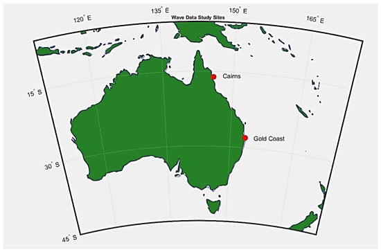
Figure 1.
Study site locations across coastal areas of Queensland, Australia.
This superior ability is enhanced with the incorporation of many neural layers to overcome problems with relatively complex function approximation due to its capability for non-linear mapping [30,31]. The problem of overfitting is also addressed with the use of hyperparameter tuning of BiLSTM parameters in the model development phase. The BiLSTM model has been successfully used in other recent studies which have shown accurate and high-quality results [32,33,34,35]. However, a hybrid Boruta random forest–ensemble empirical mode decomposition (BRF-EEMD)-BiLSTM model has not been applied in the context of sea wave forecasting to date in any previous study. Therefore, the prediction of Hs using this model is new and will provide useful insights on how sea wave parameters can help to efficiently perform short-term forecasting.
A key novelty in this study is the hybrid nature of the BiLSTM model which is incorporated with EEMD and Boruta random forest algorithms to increase the accuracy and reliability of significant wave height forecasting. It has been shown in many past studies [36,37,38] that EEMD, which is an improved version of EMD, can effectively help to break down signals into their components and mitigates modelling complexity. In [39], EEMD and long short-term memory (LSTM) algorithms have produced superior results when compared with a list of benchmark models to forecast crude oil price. In another study [40], EEMD and LSTM are combined for short-term wind speed prediction. The proposed approach in this study also outperforms other comparable models. A study [41] based on forecasting energy demand which also proposes a EEMD hybrid technique with multi-model ensemble BiLSTM shows that the hybrid-based method outperforms all the state-of-the-art techniques used for comparison. Furthermore, an EEMD-Particle Swarm Optimisation (PSO)-support vector machine (SVM) hybrid method to predict rainfall-runoff in watersheds in [37] shows that this approach effectively attains better results than the benchmark standalone model.
In addition to the data decomposition method, the uses of input selection techniques such as BRF optimiser increases the efficiency of modelling by screening and selecting the significant inputs. Feature selection is an important step in the application of machine-learning methods as datasets often have too many variables to build forecasting models [42]. An obvious reason for using a feature selection method is to overcome the computational load on algorithms by selecting more significant inputs. Due to its iterative ability, BRF can deal with the fluctuating nature of a random forest’s importance measure and the interactions between the attributes [42]. Many studies have effectively used BRF feature selection for the improvement of machine learning models. A study [43] for future soil moisture estimation successfully uses Boruta random forest (BRF) feature selection to select and capture significant inputs. The hybrid BRF-LSTM model outperforms the standalone models (LSTM, SVR and Multivariate Adaptive Regression Splines (MARS)) in this study. A similar approach is used in [44], which found superior results by a hybrid EEMD-Boruta-ELM model when forecasting soil moisture. The importance of input selection by BRF for data-driven streamflow forecasting is also demonstrated in [45].
2. Materials and Methods
2.1. Study Area and Data
This study utilised 30 min interval recorded wave features data (Table 1) for a period from 2014–2019 acquired from the Queensland government open data portal for coastal areas in Queensland. The wave features used in this study are significant wave height (Hs), maximum wave height (Hmax), zero up crossing wave period (Tz), peak energy wave period (Tp) and approximation of sea surface temperature (SST). Table 1 and Figure 1 show the selected sites and geographical location.

Table 1.
Geographical location of data site.
There are no set criteria for data partition, however datasets are normally divided into training, validation and testing. This study uses a data partition of 60% training, 20% validation and 20% testing (see Table 2) for best results.
Table 2.
Data partition for modeling.
2.2. Data Preparation
The initial step in data preparation is to identify outliers, missing and ‘incorrect’ data values in the dataset. The accuracy of data modelling depends significantly upon the accuracy and reliability of data. Outliers are data points that are in a minority and have patterns which are quite different to the majority of other data points in the sample [46]. Any presence of outliers in the data will significantly affect how the machine learning models will effectively train the model for forecasting. Cook’s distance [47] can be effectively used to detect and remove the outliers to improve any dataset for machine learning modelling. This method of removing outliers is mostly used to detect the influence of data points in a regression analysis [48]. Cook’s distance of observation is given as:
where, is the th fitted response value, is the th fitted response value when the fit excludes observation , is the mean squared error, and is the number of coefficients in the regression model. The next important step is to determine the stationarity of the time series data. In order to fit a stationary model, it is highly important to determine that the data is a realisation of a stationary process [49].
This study uses two statistical tests to confirm the stationarity of the wave data (see Table 3), the augmented Dickey Fuller (ADF) and Kwiatkowski–Phillips–Schmidt–Shin (KPSS) tests. The augmented Dickey Fuller test is for larger datasets and tests the null hypothesis that unit root is present in the data. A greater negative value of the ADF statistic than the critical value confirms that null hypothesis can be rejected, and no unit root is present. To complement the ADF test, the KPSS test can be used to confirm ADF test. If the KPSS statistic is less than the critical value, then the null hypothesis is accepted confirming that the series is stationary.
Table 3.
Augmented Dickey Fuller (ADF) and Kwiatkowski–Phillips–Schmidt–Shin (KPSS) analysis results.
The following results confirm the stationarity criteria for the Gold Coast dataset and the same procedure was used for Cairns to confirm stationarity.
Considering, Hs as the time series variable for the 30 min interval, the significant lags are then used with the other wave feature variables of zero up crossing wave period (Tz), peak energy wave period (Tp), and sea surface temperature (SST) as the inputs to predict the significant wave height (Hs) (see Table 4).
Table 4.
Input features and description.
2.3. Data Normalisation
All of the model input data were normalized [50,51,52] to make the range of [0,1] for modelling by Equation (3):
After the forecasting using the trained model, values are then returned to the original values using Equation (4).
where is the input data value, is the overall minimum and is the overall maximum value.
2.4. Data Decomposition by Ensemble Empirical Mode Decomposition (EEMD)
The EEMD method is an adaptive method that decomposes its original signal into components with amplitude and frequency-modulated parameters with a noise-assisted and analysis technique [53]. It is based on the commonly used empirical mode decomposition (EMD) which is a self-adaptive decomposition technique [54]. This method is suitable for both non-linear and non-stable signals as well. EEMD is largely improved from EMD by the addition of Gaussian white noise into the raw series. Hence, it can attribute signals with different time scales to the reference time scales.
The algorithm splits the original wave signals into intrinsic mode functions (IMFs). The training, validation and testing data are split separately by the algorithm. This is done to ensure no leakage of information occurs from the training IMFs into the validation and testing phase of modeling.
Given, n-dimensional length L of a dataset, the application in this study follows the algorithm in [54,55]. The procedure considers two important conditions:
- The n-dimensional length either has an equal number of extrema and zero crossings, or they differ at most by one.
- The mean value at any point which is defined by local maxima and the envelope defined by the local minima are zero.
The EEMD is implemented as follows [54]:
- The white noise series are added to the wave data;
- Wave dataset is then decomposed with added white noise into its IMFs (see Figure 2);
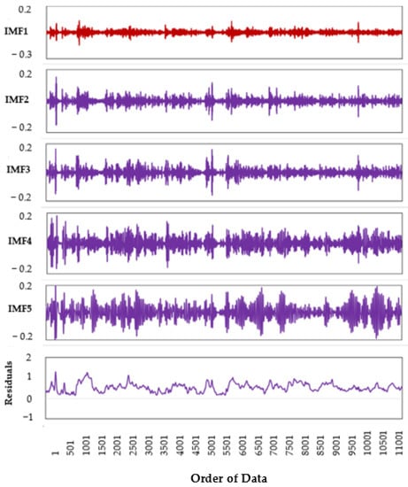 Figure 2. Temporal time-series signal of IMFs and residuals from the EEMD transformation of Hs.
 - Steps 1 and 2 are repeated with different Gaussian white noise series.
- Since the mean value of added noise is zero, the average over all corresponding IMFs will be the final decomposition.
Figure 3 shows the partial autocorrelation function (PACF) plot of the Hs time series to show the antecedent behaviour in terms of the lag of Hs in hours. The partial autocor-relation (PACF) function analysis is also used to determine the lags of the wave prediction model for the target variable Hs. The PACF analysis method is widely used as it provides partial correlation of the stationary time series with its own lagged values. It helps to de-termine how many past lags can be useful to include in the forecasting model. The de-composition of original input series of 48 lags produces 6 IMFs of each lag.
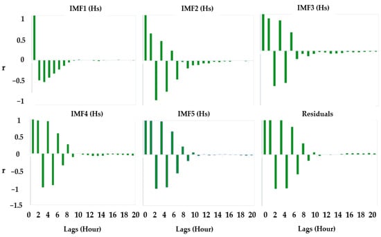
Figure 3.
Partial autocorrelation function (PACF) plot of the Hs time series exploring the antecedent behaviour in terms of the lag of Hs in hours.
2.5. Feature Selection by Boruta Random Forest Optimiser (BRF)
Boruta is a feature selection method where the algorithm is built around the random forest classification. It is based on an ensemble where selection is made according to the voting of multiple weak classifiers known as decision trees. The following steps summarize the feature selection process [42]:
- the information system is extended by the addition of all variables in consideration, minimum of five shadow attributes are added;
- the added attributes are shuffled so that their correlation with the response are removed;
- the random forest classifier is applied to gather the z-scores;
- the maximum z-score among the shadow attributes is found and every attribute that has a better score than this is taken as a hit;
- a two-sided test of equality is performed with attributes that attained an undetermined importance;
- the attributes that have significantly lower z-score than the maximum z-score among the shadow attributes are removed;
- the attributes that have significantly higher z-score are selected;
- all shadow attributes are then removed.
The correlogram in Figure 4 shows the covariance between the objective variable (Hs) in terms of the cross-correlation coefficient (rcross) for Cairns. The input lags are then selected based on their significance when the IMFs are screened by the Boruta algorithm (see Figure 5).
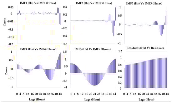
Figure 4.
Correlogram showing the covariance between the objective variable (Hs) in terms of the cross-correlation coefficient (rcross) for Cairns.
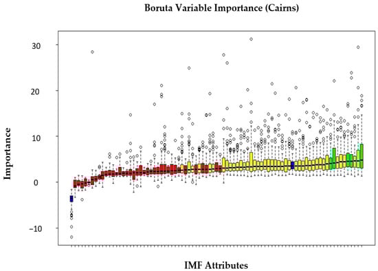
Figure 5.
Boruta feature selection output for Cairns. The intrinsic mode functions (IMFs) are compared with shadow attributes and declared as confirmed (hit) or rejected (removed) using the Boruta algorithm in R package.
Figure 6 shows the overview of the workflow for the hybrid model development. The wave predictors and target variable (Hs) pass through a series of model screening process so that significant features are extracted from the raw data.
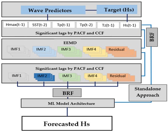
Figure 6.
Workflow detailing the steps in the model designing phase, as for the proposed hybrid EEMD-BiLSTM predictive models. Note: BiLSTM = Bidirectional Long Short-Term Memory, BRF = Boruta Random Forest Optimiser.
2.6. Modal Development
2.6.1. Bidirectional Long Short-Term Memory (BiLSTM) Model Development
Figure 7 shows the proposed BiLSTM architecture snapshot used for significant wave height modelling. The input connects to five layers, two BiLSTM layers, a unidirectional LSTM layer, a dense layer and an activation layer which finally connects to the output.
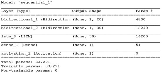
Figure 7.
A snapshot taken within the BiLSTM model development phase; it shows the layers through which the information flows for learning in the network.
Model design variables and hyperparameters are set manually with a pre-determined value before the training phase. These can be considered as ‘knobs’ which can be turned to tune the deep learning models. These values can be found by a trial and error approach, doing 100% manual search or alternatively by grid-search as in this study. Table 5 shows the model variables and hyperparameters which were used for BiLSTM.
Table 5.
BiLSTM model variables and hyperparameters obtained from grid search.
2.6.2. Support Vector Regression (SVR) Model Development
The penalty or the cost function C in SVR determines if the data are of a good quality by the narrow distance between any two hyperplanes. If the data are noisy, a smaller value of C is preferred so that support vectors are not penalised. Therefore, it is important to deduce an optimal value of C. Hence, a cross-validated grid search was done on the γ and C values, at different values of ε. For different combinations for ε, γ, and C, Table 6 shows the optimal scores obtained from the grid search procedure.
Table 6.
Optimal values obtained from grid search for ε, γ, and C in the support vector regression (SVR) model.
2.6.3. Bi-Directional Long Short-Term Memory (BiLSTM) Architecture
Each LSTM network unit is a special kind of recurrent neural network (RNN) (see Figure 8) and is an effective model for many sequential learning problems [56,57,58,59,60,61]. It was designed to model temporal information and long-term memory more than conventional RNNs. RNN is an artificial neural network and is a strong dynamic system that takes the input sequence one at a time (see Figure 9), which has the capability of holding historical information of already processed inputs in the hidden units [62]. However, the back-propagation with time method also presents an issue with vanishing and exploding gradient [63,64]. In addition to this, RNN does not have the capability to model the long-range context dependency between the inputs and outputs. Hence, to overcome these problems, LSTM was introduced which has special memory units in the hidden layer).
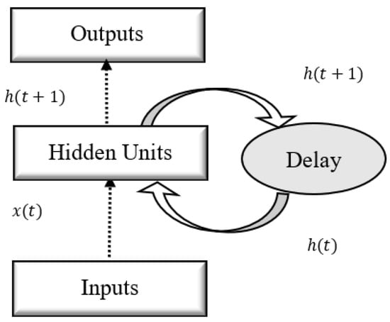
Figure 8.
The recurrent neural network diagram showing the unit arrangement.
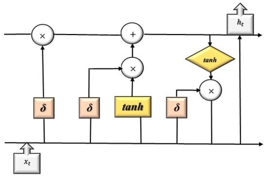
Figure 9.
The long short-term memory (LSTM) cell block representation on how the input is processed within the architecture.
The BiLSTM model (see Figure 10) is a DL network architecture and is an extension of the single unidirectional LSTM where each training sequence is fed into both, forward and backward recurrent nets that are separately connected to the same output layer. Hence, for every point in a given sequence, the network structure takes full sequential information about all points before and after [65,66]. The following gates and functions form the basis of the overall architecture:
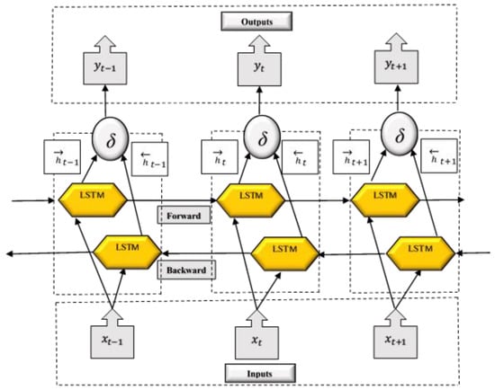
Figure 10.
The BiLSTM cell structure at time step . The architecture has the forward and backward flow arrangement of connected LSTM layers.
Forget Gates:
Input Gates:
Output Gates:
Sigmoid Function:
Cell Input State:
Hypertangent Function:
where, , , and are bias vectors. The , , , and are weight matrices which connects the previous cell output state to the gates and the input cell state. The , , , and are weight matrices that maps the hidden layer input to the gates and the input cell state. The gate activation function is sigmoid. The cell output and output at each iteration are calculated as follows:
The BiLSTM network takes data and processes it in both directions with separate hidden layers (Figure 10). It takes output from these two sequences and combines them using a merge mode which could be a concatenating ‘concat’, summation ‘sum’, average ‘ave’ or a multiplication ‘mul’ function. Finally, the sequence gives an output of prediction vectors: ,, . Each is calculated using the merge mode as follows:
The support vector (SV) algorithm was developed by Vapnik and co-workers in Russia [67]. The algorithm is based on non-linear generalisation of the generalised portrait algorithm developed in Russia in the past three decades [67,68]. The support vector machine (SVM) can also be applied using regression (SVR) and is based on the same principles (see Figure 11). This regression version was developed by Vapnik, Steven Golowich, and Alex Smola in 1997 [69]. It can be effectively used for prediction to minimize the error, find the optimum solution and avoid the “curse of dimensionality” [70].
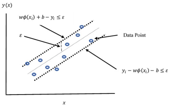
Figure 11.
The SVR model structure shows how the error and the hyperplane are arranged around the data points.
Subject to:
where C = penalty parameter, = an insensitive loss function and = slack variables.
3. Results and Discussion
Several statistical metrics were used in this study to evaluate the performance of the stacked BiLSTM and the SVR models. The commonly used model score metrics such as the Pearson’s correlation coefficient (R), Nash–Sutcliffe coefficient (NS), Willmott’s index of agreement (WI), root mean square error (RMSE), mean absolute error (MAE) and mean absolute percentage error (MAPE).
The mathematical forms are as follows:
- Pearson’s Correlation Coefficient (R)
- 2
- Nash-Sutcliffe Coefficient (NS)
- 3
- Willmott’s Index of agreement (WI)
- 4
- Root Mean Square Error (RMSE)
- 5
- Mean Absolute Error (MAE)
- 6
- Mean Absolute Percentage Error (MAPE)
Results obtained from the standalone and hybrid models for forecasting significant wave height (Hs) were assessed to validate their effectiveness in the 24 h forecasting. The forecasted values using all models in this study were analysed in terms of the predictive accuracy. The comparison was made based on the six key statistical performance criteria (Equations (13)–(18)). The performance metrics of all models in the testing phases are shown in Table 7 with the best model in bold.
Table 7.
Testing metrics results for SVR, EEMD-SVR, BiLSTM and EEMD-BiLSTM models.
For all the study locations in the testing phase of significant wave height prediction , the EEMD-BiLSTM model outperformed all other benchmark models with higher Pearson’s correlation coefficient (R) value and lower RMSE, MAPE and MAE (see Table 7). The Taylor diagram (see Figure 12) shows the statistical summary of how the observed values match with the forecasting values. Figure 12 shows the comparison of the models in terms of Pearson’s correlation, RMSE and standard deviation. The illustration shows the objective model (red dot) outperforming all other benchmark models in terms of these important performance measuring metrics.
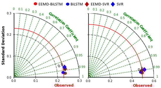
Figure 12.
Taylor diagram representing correlation coefficient together with the standard deviation difference for proposed hybrid EEMD-BiLSTM vs. benchmark models for Cairns and Gold Coast.
In addition to this, to further evaluate and validate the accuracy of the models, dimensionless metrics such as WI [71] and NS [72] have been calculated. These metrics overcome the insensitivity of correlation-based measures to differences in the observed and model-simulated means and variance [71,72,73]. WI is a dimensionless measurement of model accuracy which is bounded by 0 and 1, meaning no agreement for 0, and a perfect fit for 1 [71,74]. The values obtained show consistent higher scores of more than 95% for standalone and greater than 98% for hybrid models. NS is another normalised metric that is widely used in evaluating forecasted results [75]. It ranges from −∞ to 1, an efficiency of 1 corresponds to a perfect match of simulated data to the observed data. EEMD-BiLSTM NS achieves a value of greater than 0.95 (Figure 13), these values confirm the efficiency of the prediction models as used in many past research studies [75,76,77,78]. The curve fitting between the observed significant wave height () and predicted significant wave height () for 30-min prediction are shown in Figure 13 for both the models at the two coastal sites. The scatter plot shows the relationship between the normalized predicted and observed values. EEMD-BiLSTM provides a better curve fitting between () and (), a higher quality of fit R2 and a small residual error.
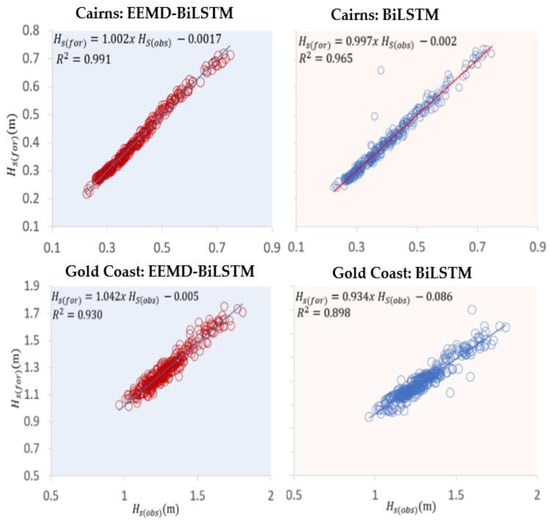
Figure 13.
Scatter plot of forecasted vs. observed Hs of Cairns and Gold Coast sites. A least square regression line and coefficient of determination (R2) with a linear fit equation are shown in each sub-panel.
The histograms in Figure 14 compare the 24 h absolute forecasting error. These show the difference between the forecasting model value and the actual value in the testing period. The EEMD models where signal decomposition was used shows high frequency of values with lower absolute forecasting error whereas the standalone models have higher absolute forecasting error with larger values. The objective model, EEMD-BiLSTM, has a lower range of forecasting error when compared with all benchmark models used in the study for both study sites.
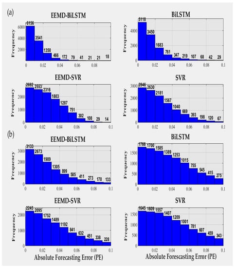
Figure 14.
Histograms of absolute forecasting error (PE) generated by EEMD-BiLSTM and the benchmark models for (a) Cairns and (b) Gold Coast data sites.
4. Conclusions
Since the physical models present many challenges of computational complexity and convergence issues of solutions, data-driven models can be an important alternative in providing ocean wave predictions and assessment. The results have shown that the hybrid EEMD-BiLSTM model that is enhanced with the Boruta feature selection optimiser can provide valuable and accurate insight into 24-hour forecasting, much needed for prior preparation for coastal wave events. This information on wave heights and notable changes in the sea level could be very helpful for assessing wave activities along coastal areas. According to [79], coastal vulnerability is in the medium range if the mean significant wave height is between 1.25 m and 1.4 m. The analysis of wave data in this study shows Gold Coast with a high frequency of Hs with height greater than 2 m when compared with Cairns. Thus, any accurate and reliable forecasting will help to ensure prior planning and preparation. The Australian Bureau of Meteorology (BOM) also uses this concept of significant wave height for warnings regarding ocean swells.
This study has also shown that a new and advanced hybrid methodology that combines two LSTM layers where LSTM units have taken the dependence between consecutive events into computation on a relevant time stamp can be effectively implemented with an effective signal decomposition and feature selection technique for the marine environment. It represents a new paradigm in significant wave height forecasting where all timesteps of the input features are utilised through the forward and backward feed network structure. To validate the merits of the proposed BRF-EEMD-BiLSTM model, a comprehensive evaluation of the model was carried out through calculation of statistical metrics and visualisation with comparison with benchmark models. Considering these results, the newly proposed hybrid model with half-hourly wave input data can be an effective tool for short-term prediction of Hs. The overall analysis and assessment of wave features at the two coastal sites of Queensland shows high wave impact and more coastal vulnerability towards the South East region. The availability of forecasting ability of artificial intelligence models such as those used in this study will further enable more reliable and accurate future wave warning systems. This study can also be extended at medium to long time-horizon forecasting.
Author Contributions
Conceptualization, N.R.; methodology, N.R.; software, N.R.; validation, N.R. and J.B.; formal analysis, N.R.; investigation, N.R.; resources, N.R.; data curation, N.R.; writing—original draft preparation, N.R.; writing—review and editing, N.R. and J.B.; visualization, N.R. All authors have read and agreed to the published version of the manuscript.
Funding
This research received no external funding.
Institutional Review Board Statement
Not applicable.
Informed Consent Statement
Not applicable.
Data Availability Statement
The data that support the findings of this study are openly available in Queensland Government Open Data Portal at https://www.data.qld.gov.au/dataset/coastal-data-system-historical-wave-data (accessed on 1 January 2020).
Acknowledgments
The paper acknowledges the Queensland Government Open Data Portal site from where the historical wave dataset for Queensland coastal areas were obtained [80].
Conflicts of Interest
The authors declare no conflict of interest.
References
- Doukakis, E. Coastal vulnerability and risk parameters. Eur. Water 2005, 11, 3–7. [Google Scholar]
- Mimura, N. Vulnerability of island countries in the South Pacific to sea level rise and climate change. Clim. Res. 1999, 12, 137–143. [Google Scholar] [CrossRef]
- Aung, T.H.; Singh, A.M.; Prasad, U.W. Sea level threat in Tuvalu. Am. J. Appl. Sci. 2009, 6, 1169–1174. [Google Scholar] [CrossRef]
- Hopley, D.; Smithers, S.G.; Parnell, K. The Geomorphology of the Great Barrier Reef: Development, Diversity and Change; Cambridge University Press: Cambridge, UK, 2007. [Google Scholar]
- Hardy, T.A.; Mason, L.B.; McConochie, J.D. A wave model for the Great Barrier Reef. Ocean Eng. 2001, 28, 45–70. [Google Scholar] [CrossRef]
- Hench, J.L.; Leichter, J.J.; Monismith, S.G. Episodic circulation and exchange in a wave-driven coral reef and lagoon system. Limnol. Oceanogr. 2008, 53, 2681–2694. [Google Scholar] [CrossRef]
- Young, I.R. Wave transformation over coral reefs. J. Geophys. Res. Ocean. 1989, 94, 9779–9789. [Google Scholar] [CrossRef]
- Hardy, T.; Young, I. Modelling spectral wave transformation on a coral reef flat. In Coastal Engineering: Climate for Change, Proceedings of the 10th Australasian Conference on Coastal and Ocean Engineering 1991, Auckland, New Zealand, 2–6 December 1991; Water Quality Centre, DSIR Marine and Freshwater: Hamilton, New Zealand, 1991. [Google Scholar]
- Wu, N.; Wang, Q.; Xie, X. Ocean wave energy harvesting with a piezoelectric coupled buoy structure. Appl. Ocean Res. 2015, 50, 110–118. [Google Scholar] [CrossRef]
- McCormick, M.E. Ocean Wave Energy Conversion; Courier Corporation: Chelmsford, MA, USA, 2013. [Google Scholar]
- Pecher, A.; Kofoed, J.P. Handbook of Ocean Wave Energy; Springer: London, UK, 2017. [Google Scholar]
- Thomsen, K. Offshore Wind: A Comprehensive Guide to Successful Offshore Wind Farm Installation; Academic Press: Cambridge, MA, USA, 2014. [Google Scholar]
- Wang, H.; Wang, J.; Yang, J.; Ren, L.; Zhu, J.; Yuan, X.; Xie, C. Empirical algorithm for significant wave height retrieval from wave mode data provided by the Chinese satellite Gaofen-3. Remote Sens. 2018, 10, 363. [Google Scholar] [CrossRef]
- Ibarra-Berastegi, G.; Saénz, J.; Esnaola, G.; Ezcurra, A.; Ulazia, A. Short-term forecasting of the wave energy flux: Analogues, random forests, and physics-based models. Ocean Eng. 2015, 104, 530–539. [Google Scholar] [CrossRef]
- Cornejo-Bueno, L.; Nieto-Borge, J.; García-Díaz, P.; Rodríguez, G.; Salcedo-Sanz, S. Significant wave height and energy flux prediction for marine energy applications: A grouping genetic algorithm–Extreme Learning Machine approach. Renew. Energy 2016, 97, 380–389. [Google Scholar] [CrossRef]
- Deo, M.; Naidu, C.S. Real time wave forecasting using neural networks. Ocean Eng. 1998, 26, 191–203. [Google Scholar] [CrossRef]
- Savitha, R.; Al Mamun, A. Regional ocean wave height prediction using sequential learning neural networks. Ocean Eng. 2017, 129, 605–612. [Google Scholar]
- Zhang, Y.; Xiong, R.; He, H.; Pecht, M.G. Long short-term memory recurrent neural network for remaining useful life prediction of lithium-ion batteries. IEEE Trans. Veh. Technol. 2018, 67, 5695–5705. [Google Scholar] [CrossRef]
- Cui, Z.; Ke, R.; Pu, Z.; Wang, Y. Deep bidirectional and unidirectional LSTM recurrent neural network for network-wide traffic speed prediction. arXiv 2018, arXiv:1801.02143. [Google Scholar]
- Carballo, J.A.; Bonilla, J.; Berenguel, M.; Fernández-Reche, J.; García, G. New approach for solar tracking systems based on computer vision, low cost hardware and deep learning. Renew. Energy 2019, 133, 1158–1166. [Google Scholar] [CrossRef]
- Wen, L.; Zhou, K.; Yang, S.; Lu, X. Optimal load dispatch of community microgrid with deep learning based solar power and load forecasting. Energy 2019, 171, 1053–1065. [Google Scholar] [CrossRef]
- Feng, C.; Cui, M.; Hodge, B.-M.; Zhang, J. A data-driven multi-model methodology with deep feature selection for short-term wind forecasting. Appl. Energy 2017, 190, 1245–1257. [Google Scholar] [CrossRef]
- Qolipour, M.; Mostafaeipour, A.; Saidi-Mehrabad, M.; Arabnia, H.R. Prediction of wind speed using a new Grey-extreme learning machine hybrid algorithm: A case study. Energy Environ. 2019, 30, 44–62. [Google Scholar] [CrossRef]
- Qin, Y.; Wang, X.; Zou, J. The optimized deep belief networks with improved logistic Sigmoid units and their application in fault diagnosis for planetary gearboxes of wind turbines. IEEE Trans. Ind. Electron. 2019, 66, 3814–3824. [Google Scholar] [CrossRef]
- Jiang, G.; He, H.; Yan, J.; Xie, P. Multiscale convolutional neural networks for fault diagnosis of wind turbine gearbox. IEEE Trans. Ind. Electron. 2019, 66, 3196–3207. [Google Scholar] [CrossRef]
- Zhang, C.-Y.; Chen, C.P.; Gan, M.; Chen, L. Predictive deep Boltzmann machine for multiperiod wind speed forecasting. IEEE Trans. Sustain. Energy 2015, 6, 1416–1425. [Google Scholar] [CrossRef]
- Wang, H.; Wang, G.; Li, G.; Peng, J.; Liu, Y. Deep belief network based deterministic and probabilistic wind speed forecasting approach. Appl. Energy 2016, 182, 80–93. [Google Scholar] [CrossRef]
- Dalto, M.; Matuško, J.; Vašak, M. Deep neural networks for ultra-short-term wind forecasting. In Proceedings of the Industrial Technology (ICIT), Seville, Spain, 17–19 March 2015; pp. 1657–1663. [Google Scholar]
- Hu, Q.; Zhang, R.; Zhou, Y. Transfer learning for short-term wind speed prediction with deep neural networks. Renew. Energy 2016, 85, 83–95. [Google Scholar] [CrossRef]
- Ghimire, S.; Deo, R.C.; Raj, N.; Mi, J. Deep solar radiation forecasting with convolutional neural network and long short-term memory network algorithms. Appl. Energy 2019, 253, 113541. [Google Scholar] [CrossRef]
- Wang, K.; Qi, X.; Liu, H.; Song, J. Deep belief network based k-means cluster approach for short-term wind power forecasting. Energy 2018, 165, 840–852. [Google Scholar] [CrossRef]
- Sun, J.; Shi, W.; Yang, Z.; Yang, J.; Gui, G. Behavioral modeling and linearization of wideband RF power amplifiers using BiLSTM networks for 5G wireless systems. IEEE Trans. Veh. Technol. 2019, 68, 10348–10356. [Google Scholar] [CrossRef]
- Zeng, Y.; Yang, H.; Feng, Y.; Wang, Z.; Zhao, D. A convolution BiLSTM neural network model for Chinese event extraction. In Natural Language Understanding and Intelligent Applications; Springer: Cham, Switzerland, 2016; pp. 275–287. [Google Scholar]
- Luo, L.; Yang, Z.; Yang, P.; Zhang, Y.; Wang, L.; Lin, H.; Wang, J. An attention-based BiLSTM-CRF approach to document-level chemical named entity recognition. Bioinformatics 2018, 34, 1381–1388. [Google Scholar] [CrossRef]
- Greenberg, N.; Bansal, T.; Verga, P.; McCallum, A. Marginal likelihood training of bilstm-crf for biomedical named entity recognition from disjoint label sets. In Proceedings of the 2018 Conference on Empirical Methods in Natural Language Processing, Brussels, Belgium, 31 October–4 November 2018; pp. 2824–2829. [Google Scholar]
- Wang, W.-C.; Chau, K.-W.; Qiu, L.; Chen, Y.-B. Improving forecasting accuracy of medium and long-term runoff using artificial neural network based on EEMD decomposition. Environ. Res. 2015, 139, 46–54. [Google Scholar] [CrossRef]
- Wang, W.-C.; Xu, D.-M.; Chau, K.-W.; Chen, S. Improved annual rainfall-runoff forecasting using PSO–SVM model based on EEMD. J. Hydroinform. 2013, 15, 1377–1390. [Google Scholar] [CrossRef]
- Zhao, H.; Sun, M.; Deng, W.; Yang, X. A new feature extraction method based on EEMD and multi-scale fuzzy entropy for motor bearing. Entropy 2017, 19, 14. [Google Scholar] [CrossRef]
- Wu, Y.-X.; Wu, Q.-B.; Zhu, J.-Q. Improved EEMD-based crude oil price forecasting using LSTM networks. Phys. A Stat. Mech. Appl. 2019, 516, 114–124. [Google Scholar] [CrossRef]
- Huang, Y.; Liu, S.; Yang, L. Wind speed forecasting method using EEMD and the combination forecasting method based on GPR and LSTM. Sustainability 2018, 10, 3693. [Google Scholar] [CrossRef]
- Javaid, N.; Naz, A.; Khalid, R.; Almogren, A.; Shafiq, M.; Khalid, A. ELS-Net: A New Approach to Forecast Decomposed Intrinsic Mode Functions of Electricity Load. IEEE Access 2020, 8, 198935–198949. [Google Scholar] [CrossRef]
- Kursa, M.B.; Rudnicki, W.R. Feature selection with the Boruta package. J. Stat. Softw. 2010, 36, 1–13. [Google Scholar] [CrossRef]
- Ahmed, A.M.; Deo, R.C.; Ghahramani, A.; Raj, N.; Feng, Q.; Yin, Z.; Yang, L. LSTM integrated with Boruta-random forest optimiser for soil moisture estimation under RCP4. 5 and RCP8. 5 global warming scenarios. Stoch. Environ. Res. Risk Assess. 2021, 1–31. [Google Scholar] [CrossRef]
- Prasad, R.; Deo, R.C.; Li, Y.; Maraseni, T. Weekly soil moisture forecasting with multivariate sequential, ensemble empirical mode decomposition and Boruta-random forest hybridizer algorithm approach. Catena 2019, 177, 149–166. [Google Scholar] [CrossRef]
- Qu, J.; Ren, K.; Shi, X. Binary Grey Wolf Optimization-Regularized Extreme Learning Machine Wrapper Coupled with the Boruta Algorithm for Monthly Streamflow Forecasting. Water Resour. Manag. 2021, 35, 1029–1045. [Google Scholar] [CrossRef]
- Hadi, A.S.; Imon, A.R.; Werner, M. Detection of outliers. Wiley Interdiscip. Rev. Comput. Stat. 2009, 1, 57–70. [Google Scholar] [CrossRef]
- Cook, R.D. Detection of Influential Observation in Linear Regression. Technometrics 1977, 19, 15–18. [Google Scholar]
- Jagadeeswari, T.; Harini, N.; Satya Kumar, C.; Tech, M. Identification of outliers by cook’s distance in agriculture datasets. Int. J. Eng. Comput. Sci. 2013, 2, 2319–7242. [Google Scholar]
- Metcalfe, A.V.; Cowpertwait, P.S. Introductory Time Series with R; Springer: Berlin, Germany, 2009. [Google Scholar]
- Kotsiantis, S.; Kanellopoulos, D.; Pintelas, P. Data preprocessing for supervised leaning. Int. J. Comput. Sci. 2006, 1, 111–117. [Google Scholar]
- Deo, R.C.; Ghimire, S.; Downs, N.J.; Raj, N. Optimization of windspeed prediction using an artificial neural network compared with a genetic programming model. In Handbook of Research on Predictive Modeling and Optimization Methods in Science and Engineering; IGI Global: Hershey, PA, USA, 2018; pp. 328–359. [Google Scholar]
- Ghimire, S.; Deo, R.C.; Downs, N.J.; Raj, N. Self-adaptive differential evolutionary extreme learning machines for long-term solar radiation prediction with remotely-sensed MODIS satellite and Reanalysis atmospheric products in solar-rich cities. Remote Sens. Environ. 2018, 212, 176–198. [Google Scholar] [CrossRef]
- Huang, N.E.; Shen, Z.; Long, S.R.; Wu, M.C.; Shih, H.H.; Zheng, Q.; Yen, N.-C.; Tung, C.C.; Liu, H.H. The empirical mode decomposition and the Hilbert spectrum for nonlinear and non-stationary time series analysis. Proc. R. Soc. Lond. Ser. A Math. Phys. Eng. Sci. 1998, 454, 903–995. [Google Scholar] [CrossRef]
- Wu, Z.; Huang, N.E.; Chen, X. The multi-dimensional ensemble empirical mode decomposition method. Adv. Adapt. Data Anal. 2009, 1, 339–372. [Google Scholar] [CrossRef]
- Lei, Y.; He, Z.; Zi, Y. Application of the EEMD method to rotor fault diagnosis of rotating machinery. Mech. Syst. Signal Process. 2009, 23, 1327–1338. [Google Scholar] [CrossRef]
- Greff, K.; Srivastava, R.K.; Koutník, J.; Steunebrink, B.R.; Schmidhuber, J. LSTM: A search space odyssey. IEEE Trans. Neural Netw. Learn. Syst. 2016, 28, 2222–2232. [Google Scholar] [CrossRef] [PubMed]
- Gers, F.A.; Schmidhuber, J.; Cummins, F. Learning to forget: Continual prediction with LSTM. In Proceedings of the 9th International Conference on Artificial Neural Networks (ICANN ’99), Edinburgh, UK, 7–10 September 1999. [Google Scholar]
- Breuel, T.M.; Ul-Hasan, A.; Al-Azawi, M.A.; Shafait, F. High-performance OCR for printed English and Fraktur using LSTM networks. In Proceedings of the 2013 12th International Conference on Document Analysis and Recognition, Washington, DC, USA, 25–28 August 2013; pp. 683–687. [Google Scholar]
- Troiano, L.; Villa, E.M.; Loia, V. Replicating a trading strategy by means of LSTM for financial industry applications. IEEE Trans. Ind. Inform. 2018, 14, 3226–3234. [Google Scholar] [CrossRef]
- Chen, Y.; Zhong, K.; Zhang, J.; Sun, Q.; Zhao, X. Lstm networks for mobile human activity recognition. In Proceedings of the 2016 International Conference on Artificial Intelligence: Technologies and Applications, Bangkok, Thailand, 24–25 January 2016. [Google Scholar]
- Mauch, L.; Yang, B. A new approach for supervised power disaggregation by using a deep recurrent LSTM network. In Proceedings of the 2015 IEEE Global Conference on Signal and Information Processing (GlobalSIP), Orlando, FL, USA, 14–16 December 2015; pp. 63–67. [Google Scholar]
- Tsoi, A.C.; Back, A. Discrete time recurrent neural network architectures: A unifying review. Neurocomputing 1997, 15, 183–223. [Google Scholar] [CrossRef]
- Bengio, Y.; Simard, P.; Frasconi, P. Learning long-term dependencies with gradient descent is difficult. IEEE Trans. Neural Netw. 1994, 5, 157–166. [Google Scholar] [CrossRef]
- Sak, H.; Senior, A.; Beaufays, F. Long short-term memory based recurrent neural network architectures for large vocabulary speech recognition. arXiv 2014, arXiv:1402.1128. [Google Scholar]
- Zhang, S.; Zheng, D.; Hu, X.; Yang, M. Bidirectional long short-term memory networks for relation classification. In Proceedings of the 29th Pacific Asia Conference on Language, Information and Computation, Shanghai, China, 30 October–1 November 2015; pp. 73–78. [Google Scholar]
- Sun, S.; Xie, Z. Bilstm-based models for metaphor detection. In Proceedings of the National CCF Conference on Natural Language Processing and Chinese Computing, Dalian, China, 8–12 November 2017; pp. 431–442. [Google Scholar]
- Basak, D.; Pal, S.; Patranabis, D.C. Support vector regression. Neural Inf. Process. Lett. Rev. 2007, 11, 203–224. [Google Scholar]
- Smola, A.J.; Schölkopf, B. A tutorial on support vector regression. Stat. Comput. 2004, 14, 199–222. [Google Scholar] [CrossRef]
- Vapnik, V.; Golowich, S.E.; Smola, A.J. Support vector method for function approximation, regression estimation and signal processing. In Advances in Neural Information Processing Systems; MIT Press: Cambridge, MA, USA, 1997. [Google Scholar]
- Liu, Y.; Wang, R. Study on network traffic forecast model of SVR optimized by GAFSA. Chaos Solitons Fractals 2016, 89, 153–159. [Google Scholar] [CrossRef]
- Willmott, C.J. On the evaluation of model performance in physical geography. In Spatial Statistics and Models; Springer: Dordrecht, The Netherlands, 1984; pp. 443–460. [Google Scholar]
- Nash, J.E.; Sutcliffe, J.V. River flow forecasting through conceptual models part I—A discussion of principles. J. Hydrol. 1970, 10, 282–290. [Google Scholar] [CrossRef]
- Legates, D.R.; McCabe, G.J. Evaluating the use of “goodness-of-fit” measures in hydrologic and hydroclimatic model validation. Water Resour. Res. 1999, 35, 233–241. [Google Scholar] [CrossRef]
- Willmott, C.J. On the validation of models. Phys. Geogr. 1981, 2, 184–194. [Google Scholar] [CrossRef]
- McCuen, R.H.; Knight, Z.; Cutter, A.G. Evaluation of the Nash–Sutcliffe efficiency index. J. Hydrol. Eng. 2006, 11, 597–602. [Google Scholar] [CrossRef]
- Jain, S.K.; Sudheer, K. Fitting of hydrologic models: A close look at the Nash–Sutcliffe index. J. Hydrol. Eng. 2008, 13, 981–986. [Google Scholar] [CrossRef]
- Coffey, M.E.; Workman, S.R.; Taraba, J.L.; Fogle, A.W. Statistical procedures for evaluating daily and monthly hydrologic model predictions. Trans. ASAE 2004, 47, 59. [Google Scholar] [CrossRef]
- Lian, Y.; Chan, I.-C.; Singh, J.; Demissie, M.; Knapp, V.; Xie, H. Coupling of hydrologic and hydraulic models for the Illinois River Basin. J. Hydrol. 2007, 344, 210–222. [Google Scholar] [CrossRef]
- Kumar, T.S.; Mahendra, R.; Nayak, S.; Radhakrishnan, K.; Sahu, K. Coastal vulnerability assessment for Orissa State, east coast of India. J. Coast. Res. 2010, 26, 523–534. [Google Scholar] [CrossRef]
- Queensland Government. Queensland Government Open Data Portal. 2019. Available online: https://www.data.qld.gov.au/dataset/coastal-data-system-historical-wave-data (accessed on 1 January 2020).
Publisher’s Note: MDPI stays neutral with regard to jurisdictional claims in published maps and institutional affiliations. |
© 2021 by the authors. Licensee MDPI, Basel, Switzerland. This article is an open access article distributed under the terms and conditions of the Creative Commons Attribution (CC BY) license (https://creativecommons.org/licenses/by/4.0/).