Assessing the Effect of Training Sampling Design on the Performance of Machine Learning Classifiers for Land Cover Mapping Using Multi-Temporal Remote Sensing Data and Google Earth Engine

Abstract

Machine learning classifiers are being increasingly used nowadays for Land Use and Land Cover (LULC) mapping from remote sensing images. However, arriving at the right choice of classifier requires understanding the main factors influencing their performance. The present study investigated firstly the effect of training sampling design on the classification results obtained by Random Forest (RF) classifier and, secondly, it compared its performance with other machine learning classifiers for LULC mapping using multi-temporal satellite remote sensing data and the Google Earth Engine (GEE) platform. We evaluated the impact of three sampling methods, namely Stratified Equal Random Sampling (SRS(Eq)), Stratified Proportional Random Sampling (SRS(Prop)), and Stratified Systematic Sampling (SSS) upon the classification results obtained by the RF trained LULC model. Our results showed that the SRS(Prop) method favors major classes while achieving good overall accuracy. The SRS(Eq) method provides good class-level accuracies, even for minority classes, whereas the SSS method performs well for areas with large intra-class variability. Toward evaluating the performance of machine learning classifiers, RF outperformed Classification and Regression Trees (CART), Support Vector Machine (SVM), and Relevance Vector Machine (RVM) with a >95% confidence level. The performance of CART and SVM classifiers were found to be similar. RVM achieved good classification results with a limited number of training samples.

1. Introduction

Land Use and Land Cover (LULC) maps are not only vital for landscape monitoring, planning, and management but also for studying the impact of climate change and human interventions on the ecosystem processes and services [1,2,3]. The term “land cover” refers to the physical cover present on the surface of the earth, whereas “land use” refers to the purpose for which the land is used. While land cover is directly amenable to remote sensing, land use can be derived by using ancillary data and expert knowledge on the characteristics of the classes available in the study area.

The most common procedure for identifying the land cover types is by classifying the remote sensing images collected by spaceborne or aerial platforms [4]. A number of classification techniques exist in the literature that can be applied to remote sensing images [5,6]. According to Yu et al. [7], the parametric Maximum Likelihood Classifier (MLC) has been the most popular technique for image classification. However, in recent times, the non-parametric machine learning (ML) classifiers have been reported to achieve better classification results for LULC [8]. Among these classifiers Random Forest (RF), Classification and Regression Trees (CART), and Support Vector Machine (SVM) proved to achieve highly accurate LULC classification results [9,10].

CART, a simple binary decision tree classifier that recursively splits the nodes until a pre-defined threshold is met [11], has been used in global LULC mapping [12]. CART’s classification accuracy and its fast performance makes it one of the widely used LULC classifiers, although it has a proven tendency to overfit [13]. This challenge can be successfully addressed by the RF classifier. RF is an ensemble classifier that consists of a user-defined number of decision trees where a subset of data is randomly extracted from training samples through replacement for building a tree, and unlabeled samples are independently classified by each tree to arrive at a collective decision through majority voting [14]. This intuitive implementation and its high accuracy results are the reasons for RF to be one of the favorite LULC classifiers [15]. SVM, on the other hand, follows a different classification approach: it builds an optimal hyperplane that separates the data such that there are minimum incorrect pixels in each class. Non-linear datasets are projected using a user-defined kernel into another higher dimensional feature before building the hyperplane. The performance of the SVM classifier depends on the defined input parameters such as the choice of kernels and defined Mercer kernel functions [16]. Despite its sensitivity to the user-defined parameters, the capability of SVM to choose a smaller subset from training samples for building the model, makes it one of the most popular classifiers in the remote sensing field [17]. A similar functional form of SVM is Relevance Vector Machine (RVM) classifier developed by Tipping [18], which uses a Bayesian framework to build a probabilistic prediction model using sparse parameters. RVM relies only on those subset of samples that has non-zero posterior probability distribution on the associated weights of hyperparameters, thus resulting in less training samples being used in the model. Previous studies proved that RVM outperformed SVM when a limited number of training samples is available [19]. Despite its clear advantages, the studies exploring the potential of RVM in remote sensing are very limited [19,20]. Furthermore, there are no studies that compared RVM and other well-known ML classifiers such as RF and CART. Deep Learning methods are also one of the important tools used for land cover classification [21]. But such methods require large, labeled datasets for training, which is not always feasible. However, recent studies such as Rostami et al. [22] and Bejiga et al. [23] provide an alternative approach to building training datasets using transfer learning methodologies that takes advantage of knowledge from existing data.

The performance of the ML classifiers is influenced by different factors including the heterogeneity/complexity of the study area, sensors’ characteristics, (e.g., spatial, temporal, spectral, and radiometric resolution), number of classes, availability of ancillary data, scale and purpose of the target land cover map, and the chosen classifier [5]. Heydari and Mountrakis [24] highlighted the importance of understanding the effect of sampling methods on land cover classification, particularly emphasizing the assessment of the impact of various sampling strategies for training data upon ML classification results, which is scarce compared to the study on testing/validation data. Among the few, Jin et al. [25] investigated how the equal and proportional sample size distribution of each class influenced the classification accuracies for urban and non-urban regions. In order to assess the effect of spatial allocation, the authors further divided each stratum into equal-sized blocks and analyzed the data distribution. Few other studies followed a data-driven approach to define strata for sampling. For example, the study by Minasny et al. [26] decomposed the area of interest into blocks with equal variability by iteratively building a variance Quadtree algorithm. Although stratification and random sampling have been the commonly used sampling methods for remote sensing applications, few studies have employed systematic sampling methods for land cover studies. Systematic sampling, widely used in the field of soils and forestry, is generally the placement of samples at equally spaced grids. For larger regions, the common method of grid creation is the confluence of latitudes and longitudes [27]. Geostatistical tools such as semi-variogram are successfully applied in systematic sampling design mainly because they provide good estimates of non-sampled locations through interpolation [28]. Van Groenigen and Stein [29] used Spatial Simulated Annealing (SSA) with the objective function Minimization of Mean Squared Distance (MMSD) to optimize the sample distribution [30]. The advantage of such geostatistical methods is that the underlying spatial variation of the variable(s) in the study area is considered and, hence, it can contribute to optimal sampling in any area of interest.

For processing the large amount of remote sensing data available today, cloud-based platforms such as Google Earth Engine (GEE) provide unprecedented computational resources that allow us to perform geospatial analysis at a global scale [31]. Many studies have leveraged the power of GEE for global LULC analysis. For example, Midekisa et al. [32] used GEE to produce annual land cover maps of 15 years over the African continent; the global forest cover change map developed by Hansen et al. [33] at 30 m resolution used multi-temporal twelve-year satellite data on GEE. Furthermore, many studies in urbanization [34,35,36], the agriculture sector [37,38,39,40], and Digital Soil Mapping [41] have also utilized GEE and its in-built ML classifiers for large and faster data processing.

The present study uses the GEE cloud platform to investigate the effect of Stratified Equal Random Sampling (SRS(Eq)), Stratified Proportional Random Sampling (SRS(Prop)), and Stratified Systematic Sampling (SSS) designs upon the LULC classification results obtained by RF classifier. In addition, we compare the performance of this classifier with CART, SVM, and RVM classifiers for land cover mapping using multi-temporal satellite remote sensing data. The research is carried out in a complex and rugged Himalayan landscape where the availability of reference data is often limited. The study addresses two major research questions: (1) what is the effect of various training sampling methods on the classification results obtained by the RF classifier? and (2) how well do the evaluated ML classifiers perform with respect to each other for land cover mapping in a complex environment? An important contribution of this work is related to the understanding the impact of stratified systematic sampling and stratified random sampling methods upon the classification results obtained by the RF classifier and evaluation of the efficiency of RVM classifier using GEE for land cover mapping.

2. Materials and Methods

2.1. Study Area and Datasets

Our study area is situated in Dehradun district lying in the northern part of India and forming a part of the Himalayan landscape (Figure 1). It covers around 3088 km² and is bound between latitudes 29°56′33″N and 30°58′30″N and longitudes 77°34′45″E and 78°18′30″E. Physiographically, the district lies in the Outer and Lower Himalayan zone. The elevation varies from about 315 to 2500 m above mean seal level. Dehradun, the district headquarters and the capital of Uttarakhand State, is located in the intermontane valley flanked by hills on its northern and southern sides. The major Himalayan Rivers, the Ganga and the Yamuna, flow along its eastern and western boundaries, respectively. The study area has a wide coverage of well-protected deciduous and evergreen forests and also comprises a large spread of plantation and agricultural lands mainly in the valley portion. The diversity of land cover classes present in Dehradun district along with the rugged nature of the terrain that limits the accessibility for field campaigns in its northern part make it a good candidate for the present study.

The datasets used in this study fall into three groups: (1) multi-temporal satellite data; (2) ancillary dataset, i.e., already existing land cover maps; and (3) high-resolution Google Earth images. Multi-temporal Landsat-8 Operational Land Imager (OLI) Surface Reflectance images of 2017 at 30 m spatial resolution formed the first group of datasets. These images are atmospherically corrected using Landsat-8 Surface Reflectance Code (LASRC) and were accessed from the GEE repository. For identifying the land cover classes present in the study area and preparing the reference data for further analysis (i.e., selecting the training and testing samples), the following available land cover maps formed the second group of datasets: (1) GlobCover map of 2015, released by the European Space Agency (ESA) at 300 m spatial resolution under the climate change initiative [42] (obtained from http://maps.elie.ucl.ac.be/CCI/viewer/index.php accessed on 7 June 2020); and (2) LULC map prepared at 1:50,000 scale under the project on Biodiversity Characterization at Landscape Level (BCLL), hereafter referred to as the BCLL-LULC map [43]. The BCLL-LULC map was generated using Indian Remote Sensing Satellite (IRS) data from 1998 to 2010. Since there is a temporal gap between the reference land cover maps used for sample generation and the satellite images used for land cover classification, we assessed the quality of the samples through visual interpretation using the high-resolution (0.5 m) Google Earth images of 2017 (https://www.google.com/earth/ accessed on 7 June 2020). Limited field campaigns have also been carried out in accessible areas during February 2019, which consisted of 22 points. The following nine land cover classes are considered in the study: deciduous forest, evergreen forest, cropland, shrubland, grassland, built-up, water bodies, river bed, and fallow land.

2.2. Methodology

The methodology used in this study is shown in Figure 2. The methodological steps include the preparation of a reference land cover map (Section 2.2.1), preparation of satellite datasets for land cover classification (Section 2.2.2), designing different sampling strategies for selecting training data (Section 2.2.3), land cover classification using different classifiers (CART, RF, SVM, and RVM) (Section 2.2.4 and Section 2.2.5), and accuracy assessment (Section 2.2.6).

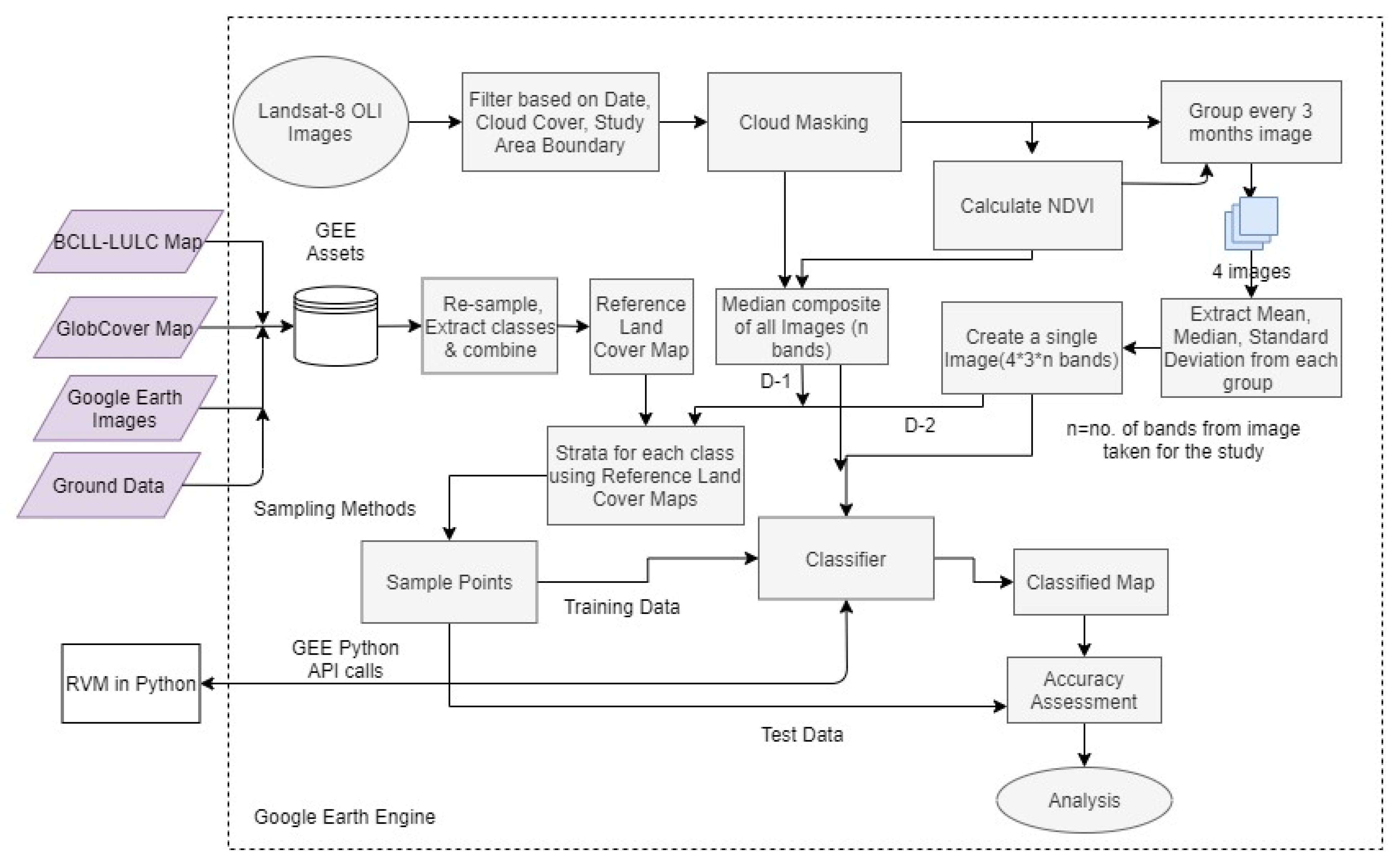
2.2.1. Preparation of Reference Land Cover Maps

Since the collection of extensive ground truth data in our study area would have been difficult, existing land cover maps (GlobCover and BCLL-LULC) were used for generating training and testing samples.

The GlobCover and BCLL-LULC maps were resampled to 30 m pixel size to match the spatial resolution of Landsat OLI images, and the land cover classes present in these maps were aggregated at the broader taxonomy level following the International Geosphere Biosphere Program’s (IGBP) land cover classification scheme [44]. Visual inspection of these land cover maps using high-resolution Google Earth images and ground data indicated some changes in the land cover classes. For example, we could detect differences between the boundaries of water bodies in GlobCover and Google Earth Images; at a few locations, shrubland was mapped as cropland in GlobCover, and there was also an overlap to some extent between the shrubland and grassland classes in both the LULC maps. The presence of croplands toward the northern part of the study area was captured well in BCLL-LULC maps. While classes such as cropland showed better visual accuracy in BCLL-LULC maps, the GlobCover map better represented the extent of Built-Up classes. Therefore, a new reference map was generated by considering one LULC map as a source of class boundary for each class. The selection of LULC map as a source for each class was done using producer and user accuracy. The producer and user accuracies of GlobCover and BCLL maps were evaluated to identify the class source and, class boundaries were extracted from that LULC map which had better class-level accuracy for a given class. This was done for six land cover classes: deciduous forest, evergreen forest, cropland, shrubland, grassland, and built-up.

As the present study considered multi-temporal data for land cover classification, three more highly dynamic, seasonal classes—water body, river bed and fallow land, were manually delineated based on the visual interpretation of the multi-temporal Landsat OLI images with high-resolution Google Earth images and field knowledge. Thus, a new reference land cover map consisting of nine classes was generated to define strata from which the training and testing samples were selected. Accuracies of the GlobCover, BCLL-LULC, and the new reference land cover map were evaluated using a test dataset containing 100 randomly selected data per class through visual interpretation of high-resolution Google Earth images, field data, and ground knowledge.

2.2.2. Preparation of Multi-Temporal Remote Sensing Data

Satellite data preparation task includes selecting Landsat-8 multi-temporal images and their integration for capturing the temporal dynamics of the target land cover classes (Figure 2). Multi-temporal Landsat-8 Operational Land Imager (OLI) Surface Reflectance (Tier 1) images of 2017 were directly accessed from the GEE repository and the clouds were masked out using the available quality bands. Considering that the land cover classes in the study area are mostly vegetation classes, Normalized Difference Vegetation Index (NDVI) is considered to help in better discrimination of land cover classes [45]. Therefore, NDVI was calculated as per Equation (1) and included as an additional input variable for the classification task.

$$NDVI=\frac{NIR-R}{NIR+R}$$

(1)

Two types of Landsat-8 datasets were created as depicted in

Table 1. Statistical dataset derived from Landsat-8 OLI 2017 images for image classification.

Dataset D-1	Median band values of B, G, R, NIR, NDVI bands
Dataset D-2	Mean, Median, Standard Deviation of B, G, R, NIR, NDVI bands within 3-month groups of 2017

. The first dataset, hereafter referred to as D-1, was created using the median values of blue (B), green (G), red (R), near-infrared (NIR), and NDVI bands (i.e., n = 5 where n denotes the number of bands in an image) for all the Landsat-8 OLI reflectance images available for 2017.

The second dataset, hereafter referred to as D-2, was created to capture the seasonal/temporal variations of the land cover classes. For this, the images were grouped at an interval of 3 months (i.e., for every quarter of the year starting from January). All images within a 3-month group were aggregated as one image containing mean, median, and standard deviation values for each band, resulting in m * n bands, where m refers to 3 aggregation types i.e., mean, median, and standard deviation. Finally, the quarterly images were further combined as a single image containing 60 bands (i.e., 4 * m * n = 4 * 3 * 5 = 60).

2.2.3. Training Data Sampling Design

The stratified sampling approach ensures the selection of samples from all available classes. Thus, the following three stratified sampling designs are studied: (1) Stratified Equal Random Sampling (SRS(Eq)); (2) Stratified Proportional Random Sampling (SRS(Prop)); and Stratified Systematic Sampling (SSS). Strata are defined based on the classes present in the reference land cover map generated as explained in Section 2.2.1. Within each stratum, training data are sampled using random (for different sample sizes) and systematic methods. The sampling units chosen are individual pixels. The effect of different sampling designs on LULC classification is further analyzed by evaluating the classification results obtained by the RF classifier, which is widely recognized as one of the best performing classifiers according to the literature [46].

To capture the possible variation in accuracies resulting from random sampling of training samples, 100 replications of sampling are implemented for each sampling design and sample size. The classification accuracies are obtained for all the trials, and average values along with their standard deviation are reported and used for assessment.

Stratified Random Sampling

Two methods are used for allocations of random samples to strata in this study. In case of SRS(Eq), the number of samples selected in each class is equal to the total number of samples divided by the number of classes. For SRS(Prop), the total number of samples is distributed into each class based on the area proportion of the land cover class in the study area. If N represents the total sample size, c represents the number of classes, A represents the total study area and a_i represents the area of class i, then every class in the SRS(Eq) method receives N/c samples and (a_i/A) * N samples in the SRS(Prop) method. The whole sampling process was performed in GEE on D-1 and D-2 satellite datasets.

In addition to different sampling strategies, we evaluated the impact of different sample sizes on classification results. To fix a starting sample size, Cochran’s formula for large populations (Equation (2)) is used by assuming an unknown proportion for each class [47]:

$$n_0=\raisebox{1ex}{$Z^{2}pq$}\!\left/ \!\raisebox{-1ex}{$e^2 ,$}\right.$$

(2)

where $n_0$ is the sample size per class, $Z$ is the $z$-value for a certain confidence, $p$ is the proportion of class in the population, $q=1-p$, and $e$ is the error margin.

For simplicity and maximum variability, $p$ is defined as 0.5, $e$ is defined as 0.05, and confidence level is defined as 95% (i.e., $Z$ = 1.96). Based on the formula, a sample set size (training + testing samples) of 358 pixels per class was considered and further varied to assess the impact upon the classification accuracy. Here, 30% of the sampled data is randomly selected from each stratum to generate the testing samples.

Stratified Systematic Sampling

Systematic sampling has the advantage of choosing samples at a constant distance from each other. This study mainly focuses on the SSA-MMSD technique to find an optimal distance between the sample points. The SSA-MMSD technique helps in obtaining the minimum distance in a class within which every non-sampled pixel can reach the sampled points. Hence, by placing the sample points at the distance obtained by this technique, we can expect the samples to be heterogeneous. The SSA-MMSD technique is mainly used here to obtain the optimal separation between sample points first and then to execute sampling at this distance, unlike in the study of Van Groenigen and Stein [29], where this technique is directly used to place the samples in a systematic grid. The semi-variance can be used to optimize the initial sampling scheme [48]. In the current study, the semi-variance parameter range is used to define the initial distribution of samples on which SSA+MMSD is applied. By placing the initial samples separated by the distance defined by the range of each class, we intend to reduce the iterations required in the SSA+MMSD technique to obtain the final solution. For classes that report a large range, the average range of all classes is used for initial distribution, as large distances do not contribute to the final solution [30]. Based on the sampling distance obtained for each class, stratified systematic sampling is performed on the datasets D-1 and D-2.

The ‘spsann’ R-programming package developed by Samuel-Rosa et al. [49] is used for implementing SSA and MMSD functionality. The initial annealing temperature is set to high values of 7000–50,000 to have a 95% acceptance probability of perturbations in the first Markov chain [30]. The MMSD obtained at the end of the annealing process for each class was used for sampling using GEE to obtain a systematic spread of samples.

2.2.4. Classification Using In-Built Classifiers in Google Earth Engine

Various image classification processes can be easily performed on GEE. The RF, SVM, and CART classifiers available in the GEE are trained using the samples obtained using the SRS(Eq) method. We selected this sampling based on its performance in this study (Section 3.3). Classifiers are tuned with different input parameters as shown in

Table 2. Input parameter values used for different classifiers available in the GEE.

Classifier	Parameter	Values	Supporting Reference
CART	Cross-Validation Factor for Pruning	5 and 10	[50]
RF	Number of Trees Number of Variables per Split	50, 100, 150, 200 Square root of input variables (√60, √5)	[46]
SVM	Kernel Type Cost Parameter SVM Type	Linear 210, 211, 3510, 212, 213, 214, 215 C_SVC	[51]

. The input parameter choice is based on the recommendations from previous literature, and the best results are used for further analysis. To obtain a more representative performance of the classifiers, the classification process is repeated for 100 trials within each sample size considered.

2.2.5. Integrating Relevance Vector Machine Classifier with Google Earth Engine

RVM is a Bayesian classifier that has the advantage of providing information on the classification uncertainties. The current study uses the faster version of RVM developed by Tipping and Faul [52] that implements a more optimized maximization of the marginal likelihood function. Based on the parameterized variables (w) of the training data (x), the Bayesian classifier builds a model with an overall aim of finding the probability distribution of target values (y). To constrain the complexity and to prevent over fitting, hyper parameter α is defined over w. For further details, refer to Shetty et al. [53]. The implementation of the classification technique is summarized as follows. The following processes (a–f) are repeated until α reduces to less than 10⁻⁴:

(a)

A polynomial basis kernel function is defined, which is initialized to 1;

(b)

A sparsity factor is calculated to determine the extent of overlap of basis vectors;

(c)

A quality factor is calculated using the variance of the kernel function with the probabilistic output of the training dataset;

(d)

The posterior probability distribution is calculated using Sigmoid and Gaussian convolution to determine α;

(e)

If α = ∞, then the corresponding basis vector is retained; and

(f)

If α < ∞ and the quality factor is less than the sparsity factor, then the basis vector is removed.

In this study, the overall RVM classification was distributed between GEE and the local computation system (Figure 3). While a verified Python implementation of the RVM classifier by Shaumyan [54] was used for classification in the local system, the process intensive tasks such as pre-processing of multi-temporal satellite images to create high-dimensional datasets and extraction of samples were performed on GEE using earth engine Python APIs.

2.2.6. Accuracy Assessment of the Classified Outputs

For evaluating the effect of sampling designs on classification accuracy and assessing the performance of classifiers, the following metrics are used: overall accuracy (OA), user accuracy, and producer accuracy. Among the various available metrics, OA is an effective, easily interpretable, and most widely used metric for accuracy estimation [55]. The user’s accuracy and producer’s accuracy, estimated from the confusion matrix, are used to further evaluate the class-level performance of a given classifier. The test sample sets are chosen through stratified random sampling using the reference land cover map such that the test and training samples are spatially disjoint.

Understanding the comparative performance of RF, CART, SVM, and RVM classifiers is another focus of the study. The relative comparison between the classifier pairs are performed using the Z-Score. With the assumption that the sample distribution is independent, the significance of comparative results (Z) of two classifiers is established by the following equation:

$$\mathrm{Z} = \frac{\left| p_1-p_{2 }\right|}{\sqrt{s_1{}^2+ s_2{}^2}} ,$$

(3)

where $p_1$ and $p_{2 }$ represent the classifier accuracies in decimals, and $s_1$ and $s_2$ denote their sample standard deviation. Given the null hypothesis, Ho: $\left| p_1-p_{2 }\right|$ = 0, and alternative hypothesis H1: $\left| p_1-p_{2 }\right|$≠ 0, the Z value is calculated for a given confidence level α/2 of a two-tailed Z-test, and the null hypothesis is rejected if Z is greater than or equal to Zα/2. In the study, the 95% confidence level is considered to compare the classifier performance such that a z-score of more than 1.96 will suggest with at least 95% probability that one classifier performs better than the other and there is only 5% probability that the successful performance could be by chance.

3. Results

3.1. Reference Land Cover Map

The average OA of the GlobCover and BCLL-LULC maps was 66.09% and 72.12%, respectively.

Table 3. Average producer and user accuracies of GlobCover, Biodiversity Characterization at Landscape Level (BCLL)-Land Use and Land Cover (LULC), new reference map, validated using test sample of 100 pixels per class. The corresponding standard deviation of accuracie values are indicated based on the variations during 100 trials (BU—Built-Up, CL—Cropland, EF—Evergreen Forest, DF—Deciduous Forest, SL—Shrubland, GL—Grassland, WB—Water Bed, RB—River Bed, FL—Fallow Land).

Land Cover Map	BU	CL	EF	DF	SL	GL	WB	RB *	FL #
	Producer’s Accuracy (%)
Globcover	89.77 ± 2.32	78.63 ± 4.33	90.88 ± 2.35	55.96 ± 1.92	46.83 ± 10.11	34.18 ± 19.41	98.11 ± 1.19	-	-
BCLL-LULC	84.28 ± 2.74	76.43 ± 2.60	91.08 ± 2.43	73.14 ± 3.25	56.66 ± 3.55	70.64 ± 8.69	96.73 ± 3.15	55.02 ± 2.26	-
New Reference	85.97 ± 2.69	77.24 ± 3.47	98.67 ± 0.94	90.51 ± 2.37	73.29 ± 2.63	58.34 ± 2.50	69.42 ± 8.65	100 ± 0.00	98.55 ± 1.07
	User’s Accuracy (%)
Globcover	100 ± 0.00	66.92 ± 3.90	85.41 ± 3.22	95.73 ± 2.66	13.55 ± 4.46	2.32 ± 1.43	100 ± 0.00	-	-
BCLL-LULC	94.32 ± 2.22	84.94 ± 3.03	97.60 ± 1.46	99.58 ± 0.66	67.81 ± 4.04	13.42 ± 3.27	41.99 ± 4.49	76.59 ± 4.50	-
New Reference	93.65 ± 2.28	94.45 ± 2.49	100 ± 0.00	97.87 ± 1.52	99.13 ± 0.83	69.16 ± 4.38	14.68 ± 3.57	100 ± 0.00	82.52 ± 3.13

* Not present in GlobCover map. ^# Not present in GlobCover and BCLL-LULC maps.

provides the producer’s and user’s accuracies of the six land cover classes in the GlobCover and BCLL-LULC maps for 100 trials. Based on these results, we selected five land cover classes (i.e., cropland, evergreen forest, deciduous forest, shrubland, and grassland) from the BCLL-LULC map and one class (i.e., built-up) from the GlobCover map. As already mentioned in Section 2.1, the river bed, water body, and fallow land were manually delineated.

The resulting reference land cover map was used for further analysis (Figure 4a). The major land cover classes occupying the study area are cropland, deciduous forest and evergreen forest, while the classes covering a relatively small portion of the landscape include grassland, water body, shrubland, river bed, built-up, and fallow land (Figure 4b).

The OA of the reference land cover map improved from 66.09 ± 1.2% and 72.12 ± 1.13% of the individual reference GlobCover and BCLL-LULC maps to 83.49 ± 0.75% for the combined reference map. Therefore, fusing existing land cover inventories proved to be a viable source for training and testing samples especially for large and inaccessible study areas where reliable and sufficient samples required for the classification of satellite images are limited or unavailable.

3.2. Effect of Sampling Design on the Classification Results

3.2.1. Stratified Random Sampling

Table 4. Average overall accuracy and standard deviation of Random Forest (RF) classified land cover map obtained for D-1 and D-2 datasets using Stratified Equal Random Sampling (SRS(Eq)) and Stratified Proportional Random Sampling (SRS(prop)) methods with different sample size (training and testing samples) for 100 trials.

Sample Size	Overall Accuracy (%) with Standard Deviation (%)
	SRS(Eq)		SRS(Prop)
	D-1	D-2	D-1	D-2
3222	63.62 ± 0.4	77.38 ± 0.4	76.07 ± 1	82.33 ± 0.9
9000	64.7 ± 0.3	78.91 ± 0.2	74.69 ± 5	81.24 ± 0.73
18,000	65.12 ± 0.27	79.28 ± 0.13	75.57 ± 0.5	83.96 ± 0.65

shows the average overall accuracies of the land cover map and their standard deviations obtained for datasets D-1 and D-2, using the SRS(Eq) and SRS(Prop) sampling methods at different sample size, each repeated for 100 trials. The SRS(Prop) method produced better OA as compared to the SRS(Eq) method (Figure 5). For a sufficiently large total sample size of 9000, which includes a large number of pixels from all classes, the SRS(Prop) method provides an approximately 6% better OA than SRS(Eq). Furthermore, the OA for dataset D-2 is in general higher as compared to dataset D-1 for different training sample sizes (Table 4) and for both sampling design methods (Figure 5). The reported standard deviation of OA results is low and < 1% for most of the sampling strategies.

The effect of training sampling design particularly in reference to the size of land cover classes is presented in Figure 6. In terms of sample composition, 11.11% of the total training sample is contributed by each class in case of SRS(Eq), while the minority classes form only 2%–5.1% of the training samples in SRS(Prop). In case of SRS(Prop), larger classes (such as deciduous forest and evergreen forest containing 37% and 20% of the training samples respectively) yielded better producer’s and user’s accuracies than the minority classes (such as shrubland and grassland that comprise 5.1% and 2% of the training samples, respectively). In contrast, minority classes have significantly higher producer’s and user’s accuracies in case of the SRS(Eq) method with an average increment in accuracy of 44% between the two methods (Figure 6a,b). On the other hand, larger classes in the SRS(Prop) method perform slightly better (an increase of +3.885% in average accuracy) than their corresponding SRS(Eq) results (Figure 6c,d). The variation of the reported user and producer accuracies for repeated experiments is low and <2.5%.

3.2.2. Stratified Systematic Sampling

In the SSS method, the sampling distance between the pixels is decided as follows: the initial distribution of training data was done using the semi-variance range values of each class. For dataset D-2, the range values varied from 216 m for fallow land to 3637 m for evergreen forest (

Table 5. Distance obtained from the range of a semi-variogram model and spatial simulated annealing (SSA) using the minimum mean squared distance (MMSD) objective function on the training sample distribution of each class for dataset D-2. For classes with very large range values such as evergreen forest, deciduous forest, and shrubland, initial sample separation is not the same as the range. For such classes, the initial sample distance taken is taken as an average class range 1500 m. The distance obtained based on SSA-MMSD is used for systematic sampling which automatically sets the sample size (BU—Built-Up, CL—Cropland, FL—Fallow Land, EF—Evergreen Forest, DF—Deciduous Forest, SL—Shrubland, GL—Grassland, RB—River Bed, WB—Water Bed).

Class	Initial Range Using Semi-Variogram (m)	Minimum Distance Using SSA+MMSD (m)	Final Training Sample Size
BU	320	280	1006
CL	504	363	2719
FL	216	186 *	450
EF	3637/1500	259 *	1092
DF	2440/1500	1057 *	377
SL	2220/1500	242	2415
GL	333	250	207
WB	1200	314	63
RB	1110	279 *	131

* Rounded off to the nearest integer.

). Classes with less intra-class variability (based on class pixel values) viz., deciduous forest, evergreen forest, and shrubland, have larger range values. However, initial sample distribution with such a large distance results in a very reduced number of training samples, which may not be a good representation of the class in a large study area. Additionally, SSA with MMSD would have taken a large execution time for such a large range. Hence, a reduced approximate average class range value of 1500 m is initially taken for the distribution of training samples in these three classes. Sampling distance was optimized by the application of SSA+MMSD, where classes such as water body and river bed experienced a reduction in sampling distance by 73.8% and 74.84%, respectively. Additionally, classes with a large range have a significantly reduced value of separation distance between training samples. With new values of separation between the samples (Table 5), a systematic sampling is performed for each class. This method also ensures that the sample size is automatically set.

The average OA of the RF classified land cover map using the SSS-based training samples is 62.36 ± 0.12% for dataset D-1 and 66.12 ± 0.12% for dataset D-2 (Figure 5). It is important to note that the OA for training samples obtained by applying only the semi-variogram range parameter values for sampling was 41.3 ± 0.3%.

Table 6. Error matrix generated using the RF classifier for the stratified systematic sampling (SSS) method with dataset D-2 and 100 validation pixels per class, during a single trial. The class-level performance in terms of producer accuracy (PA) and user accuracy (UA) is depicted under PA row and UA column (BU—Built-Up, CL—Cropland, FL—Fallow Land, EF—Evergreen Forest, DF—Deciduous Forest, SL—Shrubland, GL—Grassland, WB—Water Body, RB—River Bed).

		Reference Map
		BU	CL	FL	EF	DF	SL	GL	WB	RB	UA (%)
Classified Map	BU	74	6	3	0	0	1	5	7	5	73.27
	CL	15	65	36	5	3	11	52	7	12	31.55
	FL	1	8	60	1	4	1	0	1	0	78.95
	EF	0	6	0	79	10	9	0	0	0	75.96
	DF	0	0	0	3	59	0	2	0	0	92.19
	SL	2	14	1	12	21	77	19	7	0	50.33
	GL	0	1	0	0	3	1	22	0	0	81.48
	WB	2	0	0	0	0	0	0	77	2	95.06
	RB	6	0	0	0	0	0	0	1	81	92.05
	PA (%)	74	65	60	79	59	77	22	77	81
		Overall Accuracy: 66%

shows the error matrix for the SSS method on dataset D-2. While large classes such as forests depict good classification results, there is high confusion among cropland, grassland, and fallow land. A certain amount of overlap also exists between a spectrally similar river bed and built-up classes. Both commission and omission errors are observed in the shrubland class from many other classes.

The producer’s and user’s accuracies of SSS are consistently good for all classes. SRS(Prop) and SRS(Eq) perform 13.59% and 7.59% better than SSS respectively for datasets D-2 and D-1 (Figure 5). Although SRS methods have produced better results in most cases, the accuracies obtained from SSS are still reliable.

3.3. Performance of the Evaluated Machine Learning Classifiers

The ML classifiers (RF, CART, SVM, and RVM) were applied on Landsat OLI datasets (D-1 and D-2) for land cover classification using the training samples obtained by the SRS(Eq) method. The OA of these classifiers (for the best possible input parameter selection) versus the training sample size is shown in Figure 7. Three major observations are found. Firstly, all the evaluated classifiers show higher OA for the dataset D-2 (containing more features) as compared to dataset D-1. RF shows an average increase in OA of 14.08%, while CART shows an 11.36% increase, SVM 3.19%, and RVM 6.07% for dataset D-2. Secondly, the performance of the classifiers varies with the size of training samples. While RF and CART classifiers provided comparatively higher OA of ≈79% and ≈72%, respectively (for dataset D-2), they show a negligible change in accuracy with change in training sample size (Figure 7a,b).

On the other hand, the overall accuracies of the SVM and RVM classifiers decreased significantly when increasing the training sample size (Figure 7c,d). The maximum overall classification accuracy (for dataset D-2) is 66.74 ± 0.58% in the case of SVM and 61.29 ± 1.56% in the case of RVM for smaller sample size of 175 pixels/class. Similar results are observed for the dataset D-1 as well. Thirdly, the RF classifier consistently shows higher performance as compared to other three classifiers. The OA is obtained as 78.91 ± 0.19%, 70.63 ± 0.4%, 64.26 ± 0.64%, and 57.76 ± 1.34% for RF, CART, SVM, and RVM classifiers, respectively. The land cover maps obtained from all the four classifiers for dataset D-2 and using the training sample size of 700 pixels per class are shown in Figure 8. The analysis of producer’s and user’s accuracies revealed that the RF classifier outperformed the other classifiers even at the class level, which was followed by CART, SVM, and RVM. The producer’s and user’s accuracies of shrubland and grassland are generally found to be low in all classifiers (Figure 9). This could be due to the quality of the reference land cover map, which has been used to extract the labels of training samples.

The statistical test on comparison of classifier performance showed statistically significant difference between all classifiers except for SVM vs. CART (

Table 7. Z-test results for classifier performance comparison at 95% confidence showing two-tailed probability with test sample size of 675 pixels on dataset D-2.

RF vs. CART	RF vs. SVM	RF vs. RVM	CART vs. RVM	CART vs. SVM	SVM vs. RVM
99.998	99.997	99.998	99.855	67.822	98.942

). In all the comparisons, RF performed better than other classifiers 99% of the time, SVM performed better than RVM with 98% probability, and CART performed better than RVM with 99% probability.

3.4. Application of Relevance Vector Machine (RVM) for Land Cover Classification

The results obtained using RVM for land cover classification on Landsat OLI datasets are shown in Figure 7. It provided the highest OA of 61.29 ± 1.56% for the smallest created training sample size of 175 samples per class on dataset D-2. With the same training sample size, the OA decreased by ≈6% for the dataset D-1. The rate of decrease in the OA is initially high for a small increase in the training sample size and then gradually decreased with further increase in the training sample count. This happened because from a given training sample set, RVM selects a smaller subset of samples called relevance vectors for classifying the data. In the present study, we observed that even for a large training sample size (up to 1400 pixels per class), RVM selects only one to three relevance vectors for each class, resulting in a huge reduction in the actual training samples required for classifying the data. These final relevant vectors formed only 0.011%–0.017% of the initial sample size. The error matrix of the classified output obtained through RVM on dataset D-2 for a training sample size of 175 per class showed about 62% pixels to be correctly classified with only 20 relevance vectors (

Table 8. Error matrix obtained from the RVM classifier on dataset D-2 for sample size of 175 pixels per class for one of the trials. The number of test samples is at an average of 75 pixels per class. The class-level performance in terms of producer accuracy (PA) and user accuracy (UA) is depicted under PA row and UA column (BU—Built-Up, CL—Cropland, FL—Fallow Land, EF—Evergreen Forest, DF—Deciduous Forest, SL—Shrubland, GL—Grassland, WB—Water Body, RB—River Bed).

		Reference Map
		BU	CL	FL	EF	DF	SL	GL	WB	RB	UA (%)
Classified Map	BU	46	4	1	0	0	1	0	1	4	75
	CL	4	33	1	1	2	3	7	0	1	48
	FL	0	5	68	2	0	11	13	0	2	62.9
	EF	1	6	0	52	3	19	16	2	0	45.6
	DF	2	9	3	11	59	10	18	1	0	43.3
	SL	0	9	0	5	4	30	13	0	0	40
	GL	3	5	0	2	8	3	7	3	0	13.3
	WB	5	1	0	1	0	1	1	65	3	90.5
	RB	15	4	1	1	0	1	0	3	66	82.5
	PA (%)	47.4	32.4	82.2	62.7	60.5	30.4	5.3	90.5	93.6
	Overall Accuracy: 62.46%

). Classes such as water body and river bed were mapped well with >80% user accuracy. Most of the cropland classified pixels belonged to other natural vegetation classes or fallow land. In general, producer’s and user’s accuracies of <50% were observed in natural and managed vegetation classes.

RVM also provides additional information that helps analyze the classification errors from the posterior probability distribution of test samples into each class.

Table 9. Misclassified test samples based on posterior probability of classified output obtained through RVM (BU—Built-Up, CL—Cropland, FL—Fallow Land, EF—Evergreen Forest, DF—Deciduous Forest, SL—Shrubland, GL—Grassland, WB—Water Body, RB—River Bed).

Quartile	Posterior Probability	Misclassified Test Samples (%) in Allocated Class									Total Mis-classification (%)
	(Min–Max)	BU	CL	FL	EF	DF	SL	GL	WB	RB
Q1	0.17–0.29	4.3	5.9	2.4	4.0	15.8	3.2	4.3	1.2	1.2	42.3
Q2	0.30–0.42	0.0	1.6	3.6	10.7	5.5	8.3	5.1	1.6	4.0	40.3
Q3	0.43–0.54	0.0	0.0	5.1	4.0	0.0	0.8	0.0	0.8	2.4	13.0
Q4	0.55–0.67	0.0	0.0	2.0	0.0	0.0	0.0	0.0	0.0	2.4	4.3
Total Misclassification (%)		3.9	4.3	7.5	13.0	18.6	21.3	12.3	9.5	3.6	9.9

shows the posterior probability distribution of misclassified test samples where the probability values are distributed into quartiles, with each quartile depicting the percentage of incorrectly classified pixels. A higher probability value indicates a higher chance of a classifier misclassifying a pixel. It is evident that ≈80% of the total misclassified samples belong to the natural and managed vegetation classes, while the remaining ones belong to built-up, water body, and river bed. Built-up and water body classes are more accurately mapped as compared to other classes. Furthermore, ≈82% of the total misclassified test samples, mainly containing vegetation classes, fall in the first two quartiles (Q1 and Q2) with posterior probability ranging from 0.17 to 0.42. Only ≈13% and 4.3% of misclassified samples fall in Q3 and Q4, respectively. Fallow land and river bed are the only classes falling in Q4, suggesting that many of the classes tend to be misclassified with high probability/confidence to either fallow land or river bed. Such understanding through the probabilistic output of the RVM is critical to refine input satellite data and/or training–testing samples and, consequently the classification output.

4. Discussion

The SRS(prop) sampling method obtained better classification results for the majority of classes. Such results with proportional sampling can also be observed in studies such as Heung et al. [56], where training sampling strategies were studied for digital soil mapping. On the other hand, class-level performances of minority, i.e., infrequent, classes are found to be better for SRS(Eq) than SRS(Prop). This outcome confirms the results reported by Jin et al. [25]. Unlike SRS(Eq) and SRS(Prop), SSS relies on the class spatial variation and standard deviation to obtain the training samples using SSA and MMSD. This ensured that the SSS method performed consistently for all classes irrespective of the class size in the study area. Our study showed that the SSS method is more suitable for classes with high intra-variability (e.g., grassland) or large classes (e.g., deciduous and evergreen forests), where proportional and equal sampling can over-represent a class. Since SSS is based on the spatial distance, the training sample size is also automatically set. Additionally, the usage of MMSD helps include heterogeneous pixels in the training sample. However, SSS possesses a risk of error propagation if the first randomly chosen training sample is erroneous. Thus, given the advantages and certain disadvantages associated with each evaluated sampling method, this work proved the importance of understanding the class heterogeneity, study area, classification requirement, and the classifier for choosing the right sampling method. Furthermore, the results also account for the variation introduced by randomization of the training sample selection.

The sample size is also one of the factors that influence the results of the ML classifier. While increasing the sample size had a negligible effect on the accuracies of tree-based classifiers such as RF and CART, classifiers such as SVM and RVM showed better OA at smaller sample sizes. Similar results of RVM and SVM for smaller training sets and higher dimensional datasets can be observed in the studies by Pal and Mather [57] and Pal and Foody [19], which led the former authors to suggest using RVM as an alternative to SVM, as it uses fewer training vectors. Although a few studies (e.g., Mountrakis et al. [16]) indicated that SVM is less sensitive to sample size, the present study showed a decrease in accuracy when increasing the sample size. This may be due to the chosen input parameters viz., cost parameter, type of kernel, and training sample quality. However, further tuning of the cost parameter might help achieve better results for SVM when a larger sample size is used for training. It was observed that RVM used a very small proportion of the training samples, only 1-3 vectors per class. Our results are similar to the study reported by Pal and Foody [19], where only 1-10 relevance vectors from the training sample were involved in crop classification. This characteristic of RVM makes it an attractive classifier in areas where a limited number of high-quality training samples is available. In our study, most of the misclassified pixels fall under the lower probability quartile of posterior probability distribution. Approximately 4.5% of the test pixels were misclassified with high probability to fallow land and river bed, indicating the need for refining certain training samples. Further analysis indicated that most of the classified river bed was actually built-up class, while fallow land and deciduous forest were confused with the shrubland and grassland. Such analysis can be used to refine the input data further by adding more features and/or improving training–testing samples so that they are well separated in the feature space and away from the boundary for RVM to better discriminate the most challenging land cover classes.

Irrespective of the sample size, RF performed better compared to other classifiers, followed by CART, SVM, and RVM. Previous studies reported a similar capability of RF and SVM classifier [58]. While some earlier studies reported better performance of SVM over CART (e.g., Shao and Lunetta [59]), a few other reported vice versa (e.g., Goldblatt et al. [34]). Our results showed similar performance of both SVM and CART.

Training sample quality is another factor affecting the classifier performance. In our study, the training samples might have contained unavoidable errors due to the inherent inaccuracy of the reference land cover maps. A large study area and rough terrain posed limitations to acquire a sufficient number of good quality reference data from the field, and we had to rely mostly on the available land cover maps. Therefore, certain classes such as grassland and shrubland generally obtained producer’s and user’s accuracies of <50% for all the classifiers. The low accuracy obtained for these two classes can also be explained by the overlap of these classes with fallow land and other vegetation classes in the feature space. However, we took advantage of the presence of incorrectly labeled data to understand the classifier sensitivity to the quality of training samples. The obtained results indicated that the kernel-based SVM and RVM classifiers are more sensitive to the quality of the training samples as compared to RF and CART. Similar observations were made by Foody et al. [60] for SVM, where intentionally mislabeled training data were introduced into the training samples set. SVM’s affinity to boundary pixels and RVM’s anti-boundary nature make them more sensitive to training data quality. RF classifier, on the other hand, proved to be robust to the presence of noise in the training sample quality. Previous studies have also reported low sensitivity of RF classifier to the quality of training data [61].

Reported land cover classification accuracies were influenced by the input satellite images as well. In this study, we used two derived datasets to capture the effect of season dynamics of LULC and its influence on the classification accuracy. The study area consists of dynamic land cover classes such as cropland, shrubland, grassland, deciduous forest, water body, and river bed with high variations within a year. For example, the water body extents change significantly within a year, and the cropland in the study area consists of cereals, food grains, plantations, and pulses, and each of these crops shows a variation in growth and density during the different seasons [62]. These changes are better captured by dataset D-2, which captures variation in target land cover classes by grouping them based on different seasons. The classification accuracies are also significantly higher for D-2 when compared to D-1 (Figure 7). Therefore, a deep understanding of the temporal dynamics of the classes of interest is recommended.

Land cover classification employing multi-temporal satellite images for large study areas requires high computational resources. The GEE platform not only provided the data and computational resources but also helped in performing most of the image processing tasks through the built-in methods (i.e., RF, CART, and SVM classifiers). The integration of an externally implemented RVM classifier by distributing the pre-processing part into GEE shows the flexibility of this open cloud platform. However, additional tools to perform geo-statistical processes on GEE such as semi-variance calculations and simulated annealing need to be integrated on the platform as well.

5. Conclusions

The accuracy of classified land cover maps from remote sensing data is affected by various factors including the choice of classifiers, quality of training data, heterogeneity of the landscape, or characteristics of the input remote sensing datasets. This paper aimed at analyzing the impact of various sampling strategies upon the performance of the RF classifier for land cover mapping using multi-temporal Landsat-8 OLI data on the GEE platform. In addition, the classification results obtained by this classifier were compared to those obtained by CART, RVM, and SVM. The study is carried out in a part of the Himalayan landscape, where the availability of ground truth data is generally limited owing to rugged terrain and inaccessibility. The following conclusions and recommendations are made based on the results obtained in this study:

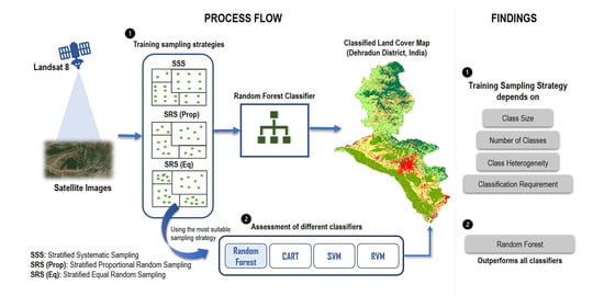
• Among the sampling techniques assessed using the RF classifier, the SRS(Prop) method produced the highest OA but obtained less satisfactory results for the underrepresented, i.e., minority, land cover classes. The SRS(Eq) method achieved a slightly lower OA but mapped minority classes with good accuracy. The performance of the SSS method increased significantly after applying the SSA+MMSD on the initial distribution of training sample points. In this method, the producer’s and user’s accuracies for all classes were consistently good for different datasets, but the OA was lower than the SRS(Eq) method. We concluded that the training sampling method should be chosen based on the class size and classification requirement: the SRS(Prop) method is recommended when the difference between the size of target classes is small, whereas the SRS(Eq) method should be applied for obtaining good accuracies at individual class levels, irrespective of their areal extent. The SSS method using SSA+MMSD techniques can be successfully used in case of large intra-class variability. Given the high performance of RF and Artificial Neural Networks for land cover mapping [21] and the importance of understanding training sampling strategies from the current work, future research is recommended to assess the effect of sampling strategies on the performance of deep neural networks. Given the limited number of training samples available for our study area, deep neural network assessments fall beyond the scope of this research.
• The RF and CART classifiers performed relatively well for different sizes of training samples. However, the SVM and RVM classifiers showed a decrease in performance when increasing the training sample size. The RF classifier outperformed other classifiers for all the training sample sizes and datasets. The performance of CART and SVM are found to be similar in this study. The potential of the RVM classifier should be further explored for land cover classification, especially due to its capability to provide information about the classification uncertainties.
• RF and CART classifiers proved to be less sensitive to the quality of training samples as compared to the kernel-based SVM and RVM classifiers. The robustness of the RF classifier to the training sample quality is as an additional advantage besides its overall higher performance.
• The performance of the RF and RVM classifiers proved to improve significantly as compared to the CART and SVM classifiers when the dataset with additional features such as seasonal variations represented by statistical measures, in terms of temporal variability in spectral signatures, was used as input variables.
• The availability of multi-dimensional remote sensing data, processing capability, and flexibility to integrate with external programs makes GEE a vital platform for land cover mapping and monitoring the change. The inclusion of geostatistical tools would further strengthen its functionality.

References

1. Luan, X.-L.; Buyantuev, A.; Baur, A.H.; Kleinschmit, B.; Wang, H.; Wei, S.; Liu, M.; Xu, C. Linking greenhouse gas emissions to urban landscape structure: The relevance of spatial and thematic resolutions of land use/cover data. Landsc. Ecol. 2018, 33, 1211–1224. [Google Scholar] [CrossRef] [Green Version]
2. Roy, P.S.; Roy, A.; Joshi, P.K.; Kale, M.P.; Srivastava, V.K.; Srivastava, S.K.; Dwevidi, R.S.; Joshi, C.; Behera, M.D.; Meiyappan, P.; et al. Development of Decadal (1985–1995–2005) Land Use and Land Cover Database for India. Remote Sens. 2015, 7, 2401–2430. [Google Scholar] [CrossRef] [Green Version]
3. Jalkanen, J.; Toivonen, T.; Moilanen, A. Identification of ecological networks for land-use planning with spatial conservation prioritization. Landsc. Ecol. 2019, 35, 353–371. [Google Scholar] [CrossRef] [Green Version]
4. Shalaby, A.; Tateishi, R. Remote sensing and GIS for mapping and monitoring land cover and land-use changes in the Northwestern coastal zone of Egypt. Appl. Geogr. 2007, 27, 28–41. [Google Scholar] [CrossRef]
5. Lu, D.; Weng, Q. A survey of image classification methods and techniques for improving classification performance. Int. J. Remote Sens. 2007, 28, 823–870. [Google Scholar] [CrossRef]
6. Khatami, R.; Mountrakis, G.; Stehman, S.V. A meta-analysis of remote sensing research on supervised pixel-based land-cover image classification processes: General guidelines for practitioners and future research. Remote Sens. Environ. 2016, 177, 89–100. [Google Scholar] [CrossRef] [Green Version]
7. Yu, L.; Liang, L.; Wang, J.; Zhao, Y.; Cheng, Q.; Hu, L.; Liu, S.; Yu, L.; Wang, X.; Zhu, P.; et al. Meta-discoveries from a synthesis of satellite-based land-cover mapping research. Int. J. Remote Sens. 2014, 35, 4573–4588. [Google Scholar] [CrossRef]
8. Ghimire, B.; Rogan, J.; Galiano, V.R.; Panday, P.; Neeti, N. An Evaluation of Bagging, Boosting, and Random Forests for Land-Cover Classification in Cape Cod, Massachusetts, USA. GIScience Remote Sens. 2012, 49, 623–643. [Google Scholar] [CrossRef]
9. Foody, G.; Mathur, A. A relative evaluation of multiclass image classification by support vector machines. IEEE Trans. Geosci. Remote Sens. 2004, 42, 1335–1343. [Google Scholar] [CrossRef] [Green Version]
10. Nery, T.; Sadler, R.; Solis-Aulestia, M.; White, B.; Polyakov, M.; Chalak, M. Comparing supervised algorithms in Land Use and Land Cover classification of a Landsat time-series. In Proceedings of the 2016 IEEE International Geoscience and Remote Sensing Symposium (IGARSS), Beijing, China, 10–15 July 2016; pp. 5165–5168. [Google Scholar]
11. Tso, B.; Mather, P.M. Classification Methods for Remotely Sensed Data, 2nd ed.; CRC Press: Boca Raton, FL, USA, 2009. [Google Scholar]
12. Friedl, M.A.; McIver, D.K.; Baccini, A.; Gao, F.; Schaaf, C.; Hodges, J.C.F.; Zhang, X.Y.; Muchoney, D.; Strahler, A.H.; Woodcock, C.E.; et al. Global land cover mapping from MODIS: Algorithms and early results. Remote Sens. Environ. 2002, 83, 287–302. [Google Scholar] [CrossRef]
13. Lawrence, R.L.; Wrlght, A. Rule-Based Classification Systems Using Classification and Regression Tree (CART) Analysis. Photogramm. Eng. Remote Sens. 2001, 67, 1137–1142. [Google Scholar]
14. Breiman, L. Random Forests. Mach. Learn. 2001, 45, 5–32. [Google Scholar] [CrossRef] [Green Version]
15. Gislason, P.O.; Benediktsson, J.A.; Sveinsson, J.R. Random Forests for land cover classification. Pattern Recognit. Lett. 2006, 27, 294–300. [Google Scholar] [CrossRef]
16. Mountrakis, G.; Im, J.; Ogole, C. Support vector machines in remote sensing: A review. ISPRS J. Photogramm. Remote Sens. 2011, 66, 247–259. [Google Scholar] [CrossRef]
17. Foody, G.M.; Mathur, A.; Sanchez-Hernandez, C.; Boyd, D.S. Training set size requirements for the classification of a specific class. Remote Sens. Environ. 2006, 104, 1–14. [Google Scholar] [CrossRef]
18. Tipping, M.E. Sparse Bayesian Learning and the Relevance Vector Machine. J. Mach. Learn. Res. 2001, 1, 211–244. [Google Scholar]
19. Pal, M.; Foody, G.M. Evaluation of SVM, RVM and SMLR for Accurate Image Classification with Limited Ground Data. IEEE J. Sel. Top. Appl. Earth Obs. Remote Sens. 2012, 5, 1344–1355. [Google Scholar] [CrossRef]
20. Foody, G.M. RVM-Based Multi-Class Classification of Remotely Sensed Data. Int. J. Remote Sens. 2008, 29, 1817–1823. [Google Scholar] [CrossRef]
21. Talukdar, S.; Singha, P.; Mahato, S.; Pal, S.; Liou, Y.-A.; Rahman, A. Land-Use Land-Cover Classification by Machine Learning Classifiers for Satellite Observations—A Review. Remote Sens. 2020, 12, 1135. [Google Scholar] [CrossRef] [Green Version]
22. Rostami, M.; Kolouri, S.; Eaton, E.; Kim, K. Deep Transfer Learning for Few-Shot SAR Image Classification. Remote Sens. 2019, 11, 1374. [Google Scholar] [CrossRef] [Green Version]
23. Bejiga, M.B.; Melgani, F.; Beraldini, P. Domain Adversarial Neural Networks for Large-Scale Land Cover Classification. Remote Sens. 2019, 11, 1153. [Google Scholar] [CrossRef] [Green Version]
24. Heydari, S.S.; Mountrakis, G. Effect of classifier selection, reference sample size, reference class distribution and scene heterogeneity in per-pixel classification accuracy using 26 Landsat sites. Remote Sens. Environ. 2018, 204, 648–658. [Google Scholar] [CrossRef]
25. Jin, H.; Stehman, S.V.; Mountrakis, G. Assessing the impact of training sample selection on accuracy of an urban classification: A case study in Denver, Colorado. Int. J. Remote Sens. 2014, 35, 2067–2081. [Google Scholar] [CrossRef]
26. Minasny, B.; McBratney, A.B.; Walvoort, D.J. The variance quadtree algorithm: Use for spatial sampling design. Comput. Geosci. 2007, 33, 383–392. [Google Scholar] [CrossRef]
27. Beuchle, R.; Grecchi, R.C.; Shimabukuro, Y.E.; Seliger, R.; Eva, H.D.; Sano, E.; Achard, F. Land cover changes in the Brazilian Cerrado and Caatinga biomes from 1990 to 2010 based on a systematic remote sensing sampling approach. Appl. Geogr. 2015, 58, 116–127. [Google Scholar] [CrossRef]
28. Montanari, R.; Souza, G.S.A.; Pereira, G.T.; Marques, J.; Siqueira, D.S.; Siqueira, G.M. The use of scaled semivariograms to plan soil sampling in sugarcane fields. Precis. Agric. 2012, 13, 542–552. [Google Scholar] [CrossRef]
29. Van Groenigen, J.W.; Stein, A. Constrained Optimization of Spatial Sampling using Continuous Simulated Annealing. J. Environ. Qual. 1998, 27, 1078–1086. [Google Scholar] [CrossRef]
30. Chen, B.; Pan, Y.; Wang, J.; Fu, Z.; Zeng, Z.; Zhou, Y.; Zhang, Y. Even sampling designs generation by efficient spatial simulated annealing. Math. Comput. Model. 2013, 58, 670–676. [Google Scholar] [CrossRef]
31. Gorelick, N.; Hancher, M.; Dixon, M.; Ilyushchenko, S.; Thau, D.; Moore, R. Google Earth Engine: Planetary-scale geospatial analysis for everyone. Remote Sens. Environ. 2017, 202, 18–27. [Google Scholar] [CrossRef]
32. Midekisa, A.; Holl, F.; Savory, D.J.; Andrade-Pacheco, R.; Gething, P.W.; Bennett, A.; Sturrock, H.J.W. Mapping land cover change over continental Africa using Landsat and Google Earth Engine cloud computing. PLoS ONE 2017, 12, e0184926. [Google Scholar] [CrossRef] [PubMed]
33. Hansen, M.C.; Potapov, P.V.; Moore, R.; Hancher, M.; Turubanova, S.A.; Tyukavina, A.; Thau, D.; Stehman, S.V.; Goetz, S.J.; Loveland, T.R.; et al. High-resolution global maps of 21st-century forest cover change. Science 2013, 342, 850–853. [Google Scholar] [CrossRef] [Green Version]
34. Goldblatt, R.; You, W.; Hanson, G.; Khandelwal, A.K. Detecting the Boundaries of Urban Areas in India: A Dataset for Pixel-Based Image Classification in Google Earth Engine. Remote Sens. 2016, 8, 634. [Google Scholar] [CrossRef] [Green Version]
35. Patel, N.N.; Angiuli, E.; Gamba, P.; Gaughan, A.; Lisini, G.; Stevens, F.R.; Tatem, A.J.; Trianni, G. Multitemporal settlement and population mapping from Landsat using Google Earth Engine. Int. J. Appl. Earth Obs. Geoinf. 2015, 35, 199–208. [Google Scholar] [CrossRef] [Green Version]
36. Trianni, G.; Angiuli, E.; Lisini, G.; Gamba, P. Human settlements from Landsat data using Google Earth Engine. In Proceedings of the 2014 IEEE Geoscience and Remote Sensing Symposium, Quebec City, QC, Canada, 13–18 July 2014; pp. 1473–1476. [Google Scholar]
37. Aguilar, R.; Zurita-Milla, R.; Izquierdo-Verdiguier, E.; De By, R.A. A Cloud-Based Multi-Temporal Ensemble Classifier to Map Smallholder Farming Systems. Remote Sens. 2018, 10, 729. [Google Scholar] [CrossRef] [Green Version]
38. Dong, J.; Xiao, X.; Menarguez, M.A.; Zhang, G.; Qin, Y.; Thau, D.; Biradar, C.; Moore, B. Mapping paddy rice planting area in northeastern Asia with Landsat 8 images, phenology-based algorithm and Google Earth Engine. Remote Sens. Environ. 2016, 185, 142–154. [Google Scholar] [CrossRef] [PubMed] [Green Version]
39. Shelestov, A.; Lavreniuk, M.; Kussul, N.; Novikov, A.; Skakun, S. Exploring Google Earth Engine Platform for Big Data Processing: Classification of Multi-Temporal Satellite Imagery for Crop Mapping. Front. Earth Sci. 2017, 5, 17. [Google Scholar] [CrossRef] [Green Version]
40. Becker, W.R.; Ló, T.B.; Johann, J.A.; Mercante, E. Statistical features for land use and land cover classification in Google Earth Engine. Remote Sens. Appl. Soc. Environ. 2021, 21, 100459. [Google Scholar] [CrossRef]
41. Padarian, J.; Minasny, B.; McBratney, A. Using Google’s cloud-based platform for digital soil mapping. Comput. Geosci. 2015, 83, 80–88. [Google Scholar] [CrossRef]
42. ESA. Land Cover CCI Product User Guide Version 2. Tech. Rep. Available online: http://maps.elie.ucl.ac.be/CCI/viewer/download/ESACCI-LC-Ph2-PUGv2_2.0.pdf (accessed on 7 June 2020).
43. Roy, P.S.; Kushwaha, S.; Murthy, M.; Roy, A. Biodiversity Characterisation at Landscape Level: National Assessment; Indian Institute of Remote Sensing, ISRO: Dehradun, India, 2012; ISBN 81-901418-8-0.
44. Loveland, T.; Belward, A. The International Geosphere Biosphere Programme Data and Information System global land cover data set (DISCover). Acta Astronaut. 1997, 41, 681–689. [Google Scholar] [CrossRef]
45. Huang, C.; Davis, L.S.; Townshend, J.R.G. An assessment of support vector machines for land cover classification. Int. J. Remote Sens. 2002, 23, 725–749. [Google Scholar] [CrossRef]
46. Belgiu, M.; Drăguţ, L. Random forest in remote sensing: A review of applications and future directions. ISPRS J. Photogramm. Remote Sens. 2016, 114, 24–31. [Google Scholar] [CrossRef]
47. J., J.E. Sampling Techniques. Technometrics 1978, 20, 104. [Google Scholar] [CrossRef]
48. McBratney, A.; Webster, R.; Burgess, T. The design of optimal sampling schemes for local estimation and mapping of of regionalized variables—I. Comput. Geosci. 1981, 7, 331–334. [Google Scholar] [CrossRef]
49. Samuel-Rosa, A.; Heuvelink, G.; Vasques, G.; Anjos, L. Spsann–Optimization of Sample Patterns Using Spatial Simulated Annealing. EGU Gen. Assem. 2015, 7780, 17. [Google Scholar]
50. Kohavi, R. A Study of Cross-Validation and Bootstrap for Accuracy Estimation and Model Selection. Int. Jt. Conf. Artif. Intell. 1995, 14, 1137–1145. [Google Scholar]
51. Yang, C.; Odvody, G.N.; Fernandez, C.J.; Landivar, J.A.; Minzenmayer, R.R.; Nichols, R.L. Evaluating unsupervised and supervised image classification methods for mapping cotton root rot. Precis. Agric. 2015, 16, 201–215. [Google Scholar] [CrossRef]
52. Tipping, M.E.; Faul, A.C. Fast Marginal Likelihood Maximisation for Sparse Bayesian Models. In Proceedings of the Ninth International Workshop on Artificial Intelligence and Statistics, Key West, FL, USA, 3–6 January 2003. [Google Scholar]
53. Shetty, S.; Gupta, P.K.; Belgiu, M.; Srivastav, S.K. Analysis of Machine Learning Classifiers for LULC Classification on Google Earth Engine; University of Twente (ITC): Enschede, The Netherlands, 2019. [Google Scholar]
54. Shaumyan, A. Python Package for Bayesian Machine Learning with Scikit-Learn API. Available online: https://github.com/AmazaspShumik/sklearn-bayes (accessed on 16 January 2018).
55. Panyam, J.; Lof, J.; O’Leary, E.; Labhasetwar, V. Efficiency of Dispatch ® and Infiltrator ® Cardiac Infusion Catheters in Arterial Localization of Nanoparticles in a Porcine Coronary Model of Restenosis. J. Drug Target. 2002, 10, 515–523. [Google Scholar] [CrossRef]
56. Heung, B.; Ho, H.C.; Zhang, J.; Knudby, A.; Bulmer, C.E.; Schmidt, M.G. An overview and comparison of machine-learning techniques for classification purposes in digital soil mapping. Geoderma 2016, 265, 62–77. [Google Scholar] [CrossRef]
57. Pal, M.; Mather, P.M. Support vector machines for classification in remote sensing. Int. J. Remote Sens. 2005, 26, 1007–1011. [Google Scholar] [CrossRef]
58. Xiong, K.; Adhikari, B.R.; Stamatopoulos, C.A.; Zhan, Y.; Wu, S.; Dong, Z.; Di, B. Comparison of Different Machine Learning Methods for Debris Flow Susceptibility Mapping: A Case Study in the Sichuan Province, China. Remote Sens. 2020, 12, 295. [Google Scholar] [CrossRef] [Green Version]
59. Shao, Y.; Lunetta, R.S. Comparison of support vector machine, neural network, and CART algorithms for the land-cover classification using limited training data points. ISPRS J. Photogramm. Remote Sens. 2012, 70, 78–87. [Google Scholar] [CrossRef]
60. Foody, G.M.; Pal, M.; Rocchini, D.; Garzon-Lopez, C.X.; Bastin, L. The Sensitivity of Mapping Methods to Reference Data Quality: Training Supervised Image Classifications with Imperfect Reference Data. ISPRS Int. J. Geo-Inf. 2016, 5, 199. [Google Scholar] [CrossRef] [Green Version]
61. Mellor, A.; Boukir, S.; Haywood, A.; Jones, S. Exploring issues of training data imbalance and mislabelling on random forest performance for large area land cover classification using the ensemble margin. ISPRS J. Photogramm. Remote Sens. 2015, 105, 155–168. [Google Scholar] [CrossRef]
62. Tuteja, U. Baseline Data on Horticultural Crops in Uttarakhand; Agricultural Economics Research Centre, University of Delhi: Delhi, India, 2013. [Google Scholar]
Figure 1. The study area, Dehradun district shown as a false color composite of surface reflectance images (bands 2, 3, and 4 depicted in blue, green, and red colors, respectively) of 2017, where a median composite image is created using all the Landsat-8 Operational Land Image (OLI) images.
Remotesensing 13 01433 g001
Figure 2. Overall methodology implemented in the study, mostly using Google Earth Engine (GEE).
Remotesensing 13 01433 g002
Figure 3. Roles of the local system and GEE for implementation of the Relevance Vector Machine (RVM) classifier.
Remotesensing 13 01433 g003
Figure 4. (a) Reference land cover map prepared in this study and (b) area-wise distribution of land cover classes (excluding the “no data” area).
Remotesensing 13 01433 g004
Figure 5. Average overall accuracy values of RF classified land cover map obtained for different sampling methods and datasets D-1 and D-2. The overall sample size for SRS(Eq) and SRS(Prop) are taken as 9000, while that for SSS is taken as 8460. The error bars indicate the standard deviation of overall accuracy for 100 trials.
Remotesensing 13 01433 g005
Figure 6. Average producer’s and user’s accuracies of smaller (a,b) and larger (c,d) land cover classes for different sampling methods obtained using the RF classifier. The error bars indicate the standard deviation of overall accuracy for 100 trials. Sample sizes of 9000 and 8460 are taken for stratified random sampling methods (SRS(Prop) and SRS(Eq)) and the stratified systematic sampling method (SSS), respectively.
Remotesensing 13 01433 g006
Figure 7. Average overall accuracy obtained for different classifiers using different training sample sizes per class and datasets (D-1, D-2): (a) RF classifier, (b) Classification and Regression Trees (CART) classifier, (c) Support Vector Machine (SVM) classifier, and (d) RVM classifier. The error bars indicate the standard deviation of overall accuracy for 100 trials.
Remotesensing 13 01433 g007
Figure 8. Land cover maps obtained using different Maximum Likelihood (ML) classifiers from dataset D-2: (a) RF classifier, (b) CART classifier, (c) SVM classifier, and (d) RVM classifier. Training samples of 700 pixels per class obtained using SRS(Eq) method are used for land cover classification.
Remotesensing 13 01433 g008
Figure 9. Average producer’s and user’s accuracies of Shrubland and Grassland for RF, CART, SVM, and RVM classifiers on dataset D-1 and D-2. The label above the bar shows the respective accuracy values, and their error bar indicates the standard deviation for 100 trials.
Remotesensing 13 01433 g009