Abstract
Two main approaches are used in mapping rice paddy distribution from remote sensing images: phenological methods or machine learning methods. The phenological methods can map rice paddy distribution in a simple way but with limited accuracy. Machine learning, particularly deep learning, methods that learn the spectral signatures can achieve higher accuracy yet require a large number of field samples. This paper proposed a pheno-deep method to couple the simplicity of the phenological methods and the learning ability of the deep learning methods for mapping rice paddy at high accuracy without the need of field samples. The phenological method was first used to initially delineate the rice paddy for the purpose of creating training samples. These samples were then used to train the deep learning model. The trained deep learning model was applied to map the spatial distribution of rice paddy. The effectiveness of the pheno-deep method was evaluated in Jin’an District, Lu’an City, Anhui Province, China. Results show that the pheno-deep method achieved a high performance with the overall accuracy, the precision, the recall, and AUC (area under curve) being 88.8%, 87.2%, 91.1%, and 94.4%, respectively. The pheno-deep method achieved a much better performance than the phenological alone method and can overcome the noises in the training samples from the phenological method. The overall accuracy of the pheno-deep method is only 2.4% lower than that of the deep learning alone method trained with field samples and this difference is not statistically significant. In addition, the pheno-deep method requires no field sampling, which would be a noteworthy advantage for situations when large training samples are difficult to obtain. This study shows that by combining knowledge-based methods with data-driven methods, it is possible to achieve high mapping accuracy of geographic variables using remote sensing even with little field sampling efforts.
1. Introduction
Paddy rice is one of the world’s major food crops and it feeds about half of the global population. The spatial distribution of rice paddy is not only the basis for decision-making in agricultural production, such as crop management, but also the basic data for agricultural research and application, such as paddy rice yield estimation and planting structure adjustment and optimization. Therefore, accurate and effective mapping of rice paddy distribution is helpful to timely and effective monitoring of paddy rice agricultural information, which can improve food crop production and ensure food security. Recently, remote sensing technology has been widely used to map rice paddy distribution, and thus has become an important research issue in agricultural monitoring of paddy rice.
The methods using remote sensing to map rice paddy distribution can be generally divided into two main categories: methods based on knowledge of paddy rice phenology (phenological methods) and those only based on spectral learning. Phenological methods are based on the cyclic and seasonal growing patterns that crops show along their respective life cycle [1]. Paddy rice has its unique phenological characteristics. For example, during the period of flooding and transplanting, the land surface of rice paddy is covered with the mixture of water, paddy rice, and soil, while other crops and dry land are usually not covered with water. Phenological methods use these characteristics to differentiate rice paddy from other crops. The phenological characteristics can usually be reflected through time series of remote sensing indices calculated from multi-temporal remote sensing images [2,3,4,5,6]. There are two representative methods that have been widely used for this purpose.
The first is based on the reflectance nature of the flooding and transplanting dates [2]. The rice paddy is mainly covered with water during this time compared with non-rice paddy areas (areas whose land cover types are not rice paddy). This method uses the Normalized Difference Water Index (NDWI) and the Normalized Difference Vegetation Index (NDVI) from remote sensing images to depict the differences between rice paddies and non-rice paddy areas. It is believed that during the flooding and rice transplanting period, the NDWI value will come close to or even slightly bigger than the value of NDVI, compared with non-rice paddy areas. In other periods, the NDWI will be smaller. The method uses a time-series of remote sensing images to analyze the phenological changes of NDWI and NDVI. These changes will be used to map rice paddy distribution. However, the success of this method can be impacted by precipitation. The areas flooded after precipitation are likely to be falsely recognized as rice paddy. Thus, the resultant distribution map can be exaggerated if the remote sensing images are acquired right after precipitation during flooding and transplanting seasons.
The second method is based on the comprehensive consideration of vegetation phenology and surface water change [3]. This method takes the characteristics of development periods aside from the rice transplanting period into consideration. They believe that from the tillering to heading period, the change of Land Surface Water Index (LSWI) is smaller while the change of two-band Enhanced Vegetation Index (EVI2) is larger, compared to other crops. Therefore, this method uses the ratio between the changing amplitude of LSWI and the difference between the EVI2 on the tillering date and the heading date to identify the rice paddy through a threshold. This method is not dependent on the short transplanting period, rather over the major periods of paddy rice life cycle. Therefore, it is more robust under the disturbance of precipitation. However, the values used for paddy rice identification constructed with phenological characteristics are simple ratios, which would not be applicable over complicated areas because it would change with different vegetation environments.
Spectral learning methods are purely based on the spectral signatures of rice paddy. The spectral learning methods can be grouped into three general types. The first type uses classic statistical methods to map rice paddy distribution [7,8,9,10,11]. Classic statistical methods usually extract distinguishable spectral signature values of the rice paddies first, and then divide the feature space according to the principle of statistical decision-making to identify paddy rice. The classic statistical classification relies heavily on the statistical characteristics (signature) of spectral data from remote sensing images. When the spectral signature of rice paddies is not distinct (unique), this type of methods is less effective.
The second type utilizes the machine learning methods [12,13,14,15,16,17]. Currently, the machine learning methods commonly used in mapping rice paddy distribution include random forest, support vector machine, and neural networks. These methods first train classification models to learn the hidden features in the spectral data from a large amount of training samples and then the trained models (trained trees, trained forests, trained vector machines, or trained networks) are applied to map rice paddy distribution from remote sensing images. For machine learning methods, theoretically, models with more parameters are more capable of learning complex patterns. The key requirement of machine learning methods is the large set of training samples, which is often obtained through field sampling.
The third type is deep learning. Deep learning is a further development of the neural networks. It contains more hidden layers than regular neural networks, capable of representing the complex relationships in a progressive and layered manner. It has more nonlinear transformations and a better generalization capability, thus can extract deeper hidden features in spectral data. It has received wide attention in the field of mapping rice paddy with remote sensing and has achieved better performance than the machine learning techniques [18,19,20]. However, deep learning, like other machine learning methods, requires a large number of training samples which are expensive and difficult to acquire.
As stated above, the phenological methods are simple but accuracy is low, the spectral learning methods, especially the deep learning methods, have strong feature learning ability and can improve the model performance. However, these methods rely heavily on a large number of training samples. It might be possible to combine the simplicity of the phenological methods with the learning ability of the deep learning methods to improve the efficiency and accuracy of rice paddy distribution mapping with remote sensing without field sampling.
Contributions
This paper aims to propose a method for mapping rice paddy distribution by coupling a phenological method with a deep learning method (referred to as pheno-deep method hereafter). The basic idea is to use the phenological method to extract initial samples from remote sensing images and then use these samples to train the deep learning model. Finally apply the trained model to map rice paddy distribution. The pheno-deep method is expected to achieve high mapping accuracy without field sampling efforts. This method also explores the feasibility of combining knowledge-based method and data-driven method for the spatial prediction of geographic variables in general.
The remainder of the article is divided into five sections. Section 2 presents the pheno-deep method. The experiment design (including case study and evaluation) is illustrated in Section 3. Section 4 contains the results, and the discussions is presented in Section 5. Section 6 draws the conclusions.
2. The Pheno-Deep Method
The pheno-deep method consists of three major steps and the overall workflow is illustrated in Figure 1. First, the phenological method is used to determine phenological characteristics and classify the cell locations into rice paddies and non-rice paddy areas based these characteristics. Second, training samples are collected from the results of phenological method for deep learning model. Third, a deep learning model is constructed and trained using the samples so acquired for mapping rice paddy.
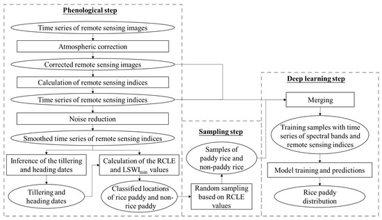
Figure 1.
The overall workflow of the pheno-deep method.
2.1. Classification of Rice Paddy Based on Phenological Method
The growing process of paddy rice can be divided into two major stages: the growth stage and the reproductive stage. The growth stage includes seedling, transplanting, and rice tillering. At this stage, the paddy rice grows rapidly, so is its vegetation coverage. Over this stage the surface is covered with mixture of water, paddy rice, and soil. The reproductive stage consists of heading and ripening. During this stage, the leaves age and turn yellow, its vegetation coverage begins to decline. These phenological characteristics can usually be reflected in time series of remote sensing images.
The phenological method proposed by Qiu et al. [3] is used to capture these phenological characteristics and map the preliminary distribution of rice paddy areas. In this method, the two-band (the red and the infrared bands) enhanced vegetation index [21] (EVI2) and the land surface water index [22] (LSWI) to characterize the phenological characteristics of paddy rice. EVI2 is used for the detection for vegetation growth status and coverage. It is calculated with the reflectance of near-infrared (NIR) and red (R) bands of remote sensing images:
EVI2 = 2.5 ∗ (NIR − R)/(NIR + 2.4 ∗ R + 1),
LSWI is sensitive to the surface moisture changes and is commonly used to detect changes in soil moisture and vegetation moisture content. It is calculated with near-infrared (NIR) and shortwave-infrared (SWIR) bands of the remote sensing images:
LSWI = (NIR − SWIR)/(NIR + SWIR),
During the paddy rice growing process, the changes of water and vegetation in the fields are two key factors reflecting the changes of paddy rice. EVI2 can be used to effectively detect the changes of vegetation while LSWI can effectively detect the changes of water content. Therefore, the time series of these two remote sensing indices can capture well the changes of paddy rice in the whole growing process. Due to the noise resulting from varying atmospheric conditions and other factors, a noise reduction process is needed to smooth the time series of LSWI and EVI2 for further computation.
The determination of a cell location to be a rice paddy or not depends on the values of two indices. The first is the ratio of change amplitude of LSWI from tillering to heading to the difference between EVI2 at a prescribed tillering date and at a heading date. This index is referred to as RCLE (Ratio of Change amplitude of LSWI to EVI2) [3], as shown in Equation (3):
RCLE = (LSWImax − LSWImin)/(EVI2heading − EVI2tillering),
The LSWImax and LSWImin are the maximum and minimum values of the LSWI between tillering and heading dates, while EVI2heading and EVI2tillering are the values of EVI2 at heading date and tillering date. The heading date for a given cell location was recognized as the date when EVI2 value reaches the primary maximum and the tillering date was set to be 40 days ahead of that [3]. The second is the minimum LSWI value from tillering date to heading date. It is referred to as LSWImin and is used to state the minimum value to be maintained for rice paddy. For a cell location to be rice paddy, the RCLE must be less than a prescribed threshold while LSWImin must be greater than another prescribed threshold [3].
2.2. Collection of Training Samples
After the rice paddy cell locations in the study area are identified using the phenological method discussed above, samples are collected based on the phenological results. The purpose of sampling is not just to obtain samples but also to increase the representativeness of the samples. Previous studies [23,24,25,26] have indicated that even for locations classified as a particular class, their respective representativeness of that class are different for different locations. Thus, it is expected that the locations classified as rice paddies and non-rice paddy areas based on the phenological method would exhibit the same nature. The different levels of representativeness can be indicated by their respective RCLE values. The smaller the RCLE the more representative to rice paddy while the larger the RCLE the more representative to non-rice paddy.
Therefore, intervals of RCLE values are designated to confine the area over which samples for rice paddy and non-rice paddy will be drawn, respectively, to increase the representativeness of the collected samples. Random sampling method is used to obtain the samples from areas whose RCLE values are within the selected ranges. Each sample consists of the tag of rice paddy or non-rice paddy and the time series of remote sensing indices and spectral bands from remote sensing images.
2.3. Deep Learning Model for Mapping Rice Paddy
The deep learning architecture used in the pheno-deep method is the Long Short-Term Memory [27] (LSTM). The LSTM is a modification to recursive neural network (RNN). In RNN, the current status is dependent on all previous status, making it suitable for processing time series data. However, as the time series gets longer, the influence of initial status becomes faint as the time series progresses. The LSTM network is designed to solve this problem by dividing stored information into long-term memory and short-term memory. The structure of the basic LSTM unit is illustrated in Figure 2. As is shown in Figure 2, an LSTM unit consists of a cell state, a forget gate, an input gate, and an output gate. The cell state keeps track of the long-term memory, including that of the previous unit (ct−1) and the output long-term memory of this unit (ct). When the input data (xt) enters the LSTM unit, it first goes through the forget gate together with short-term memory from the previous unit (ht−1). The forget gate decides the extent to which the long-term information (ct−1) remains. Then, the input data goes through the input gate where the extent to which the new information needs to be stored in long-term information is decided. Finally, the input data goes through the output gate which controls the output of new long-term memory (ct) and new short-term memory (ht). The σf in Figure 2 represents activation function, while the tanh refers to hyperbolic tangent function. The divided store of long-term and short-term memory enables more delicate computing process in LSTM unit, which makes LSTM network suitable for long time series data analysis. In this paper the input data for deep learning model is the time series of remote sensing indices and spectral bands. Therefore, the LSTM networks serve as an excellent basis to construct the deep learning model for mapping rice paddy distribution.
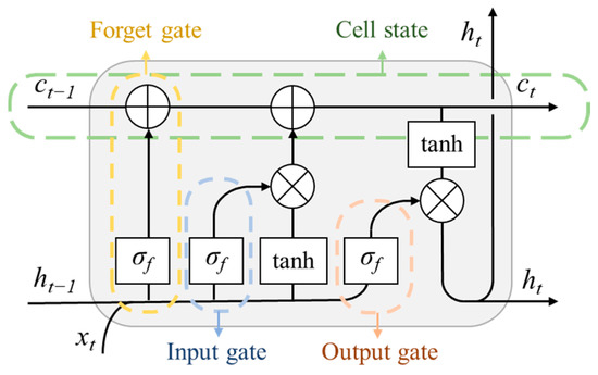
Figure 2.
The architecture of Long Short-Term Memory (LSTM) unit.
The deep learning model implementing the LSTM networks consists of four main components: the input layer, the stacked LSTM layers, the dense layer, and the output layer. The samples consisting of labels and time series of remote sensing indices and spectral bands are used as the input data. The input layer transfers the time series data of the samples to the hidden LSTM layers. The stacked LSTM layers then stack multiple LSTM units into a deep architecture. This architecture improves the network ability of representing time series data. The final output of the stacked LSTM units goes into the dense layer. In this layer, the number of computational nodes is the same as the number of predicted classes (rice paddy and non-rice paddy area in this case). It bases on activation function to convert the output from the stacked LSTM layers into a probability distribution of the predicted classes. Finally, the output layer assigns the cell to a class which has the higher probability for this cell.
3. Experiment Design
3.1. Study Area and Data Collection
The study area is Jin’an District, Lu’an City, Anhui Province, China (Figure 3). It is about 1657 km2 and is part of the Jianghuai watershed. It sits at the humid subtropical climate zone. The southern part of the study area is mostly of mountain terrains, while the central part consists of low hills and northern part is occupied mainly by plains. According to the Statistic Yearbook [28], cropland is the main land use type in the study area, accounting for approximately 68.3%, and paddy rice is the main crop, accounting for 45.7% of the crop land.
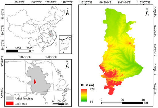
Figure 3.
Study area at Jin’an District, Anhui Province, China.
Between May and October in 2017, 17 remote sensing images of the study area from the Sentinel-2A were selected as the sources for remote sensing indices and spectral bands data. The acquisition date of each image is presented in Table 1. The selected period was the time when the middle-season rice, which is the main type of paddy rice planted in the study area, was bred and harvested. The remote sensing images were atmospherically corrected using the Py6S method [29,30]. A total of 1364 samples were acquired through field sampling with ground sampling distance being 1 m between 22 July and 24 July. Among them, 364 samples (182 for rice paddy and 182 for non-rice paddy) were used as validation samples. The remainder, that is 1000 field samples with 500 for rice paddy and 500 for non-rice paddy, were reserved for training a deep learning method which was used to compare with the pheno-deep method. None of these samples were used for the development of the pheno-deep method.

Table 1.
The acquisition dates of the used Sentinel-2A images.
3.2. Implementation of the Pheno-Deep Method
3.2.1. Rice Paddy Distribution from Phenological Method
The preliminary distribution of rice paddy, from which training samples would be selected, was mapped with the phenological method as described in Section 2.1. First, the time series of the remote sensing indices, including the EVI2 and LSWI, was computed from the 17 remote sensing images. In order to reduce the noises in the data, a Whittaker Smoother [31] was used to smooth the time series data. The smoothed time series of remote sensing indices were then used to identify the tillering and heading dates and calculate the RCLE values. The threshold for RCLE values was set to 0.9 and the threshold for LSWImin values was set to 0.1 based on previous research [3] and the climate conditions in the study area. The cell locations with RCLE value smaller than the RCLE threshold and with LSWImin value greater than the threshold of LSWImin were identified as rice paddies. Other locations were considered as non-paddy rice areas.
3.2.2. Sampling from the Phenological Results
To increase representativeness of the selected samples, RCLE ranges were set for selecting samples as stated in Section 2.2. To better capture the levels of representativeness, the RCLE values need to have an easily interpretative range (such as 0–1). However, the current RCLE value does not have an upper bound, thus RCLE needs to be normalized into a fixed range [0, 1]. For easy interpretation, 0.5 of the normalized RCLE will be set as the middle point between rice paddy and non-rice paddy. The normalization was conducted in the following way: the current RCLE values which are below 0.9 were normalized into the range of 0.0–0.5 while the RCLE values greater than 0.9 were normalized into the range of 0.5–1.0 through histogram stretching. Thus, classified locations with normalized RCLE values falling into 0.0–0.5 served as candidates for rice paddy samples while classified locations with normalized RCLE between 0.5 and 1.0 served as candidate for non-rice paddy samples. Clearly, the locations with their normalized values closer to 0.0 is more typical of rice paddies and the locations with the normalized RCLE values closer to 1.0 are more typical of non-rice paddy areas.
The normalized RCLE range between 0.2 and 0.3 was selected as the interval over which the rice paddy samples were collected, and 0.7 and 0.8 as the interval over which the samples of non-rice paddy were collected. The intervals were chosen under two considerations: (1) locations with the normalized RCLE value close to 0.5 do not represent either class well, because they are too close to the classification boundaries; (2) locations with normalized values too close either to 0.0 or to 1.0 are too pure for the respective classes and would not represent the varying nature of each classes well. Thus, they are less representative. Therefore, a range somewhat in the middle of each class variation was selected for sampling. The impact of these sampling intervals will be discussed in later in Section 5.2. In the sampling step, 350 rice paddy (positive) samples were randomly selected from cell locations where the normalized RCLE value is within the range of 0.2–0.3 and the LSWImin value is bigger than 0.1, and another 350 non-rice paddy (negative) samples from the cell locations where the normalized RCLE value is in the interval of 0.7–0.8 for model training.
3.2.3. LSTM Training and Mapping
The collected 700 samples (350 positive samples and 350 negative samples) were then used to train the model as described in Section 2.3. Each sample is assigned with a feature vector that consists of the time series of spectral bands and remote sensing indices from the 17 time series images. The blue, green, red, near infrared, and shortwave infrared were used as spectral bands. The normalized difference vegetation index [32] (NDVI), EVI2, and LSWI are used as remote sensing indices. This resulted in each sample containing a label (rice paddy or not) and a time series of 136 values (17 time series images with each containing 5 spectral bands and 3 remote sensing indices).
The LSTM model was implemented in Keras, a deep learning API based on the machine learning platform Tensorflow using Python language [33].The key hyperparameters for training the model, such as learning rate, learning rate decay, number of hidden layers and dropout value, were set based on common practice in deep learning research. The initial learning rate is set to 0.001 and the learning rate decay to 0.0001. The number of hidden layers is set to 4 considering computation time and model performance. The activation function is sigmoid [34], which is commonly used to compute probability of binary classification. The optimizer is Adam [35]. The focal loss function [36] is set as the loss function.
3.3. Evaluation Metrics
The pheno-deep method was compared with the deep learning method (deep learning alone, hereafter) and the phenological method (phenological alone, hereafter), respectively. The deep learning alone method used the same LSTM model structure and parameter settings as used in the pheno-deep method but trained using field collected samples. The training samples for the deep learning alone method were drawn from the 1000 field samples. Each time 700 (350 rice paddy and 350 non-rice paddy) from the 1000 field samples are randomly selected as training samples for the deep learning alone method. The pheno-deep method was trained using 700 samples (350 rice paddy and 350 non-rice paddy) which were randomly selected from the results based on the phenological method. The experiment for the pheno-deep method and the deep learning alone method are each repeated for 50 times with different training samples as outlined above.
For the comparison with the phenological alone method, the feature vector of the training samples used in the pheno-deep method consists of only the time series of LSWI and EVI2 so that the data used in the phenological method and the pheno-deep method are the same. For the pheno-deep method with only LSWI and EVI2 data, 700 samples (350 rice paddy and 350 non-rice paddy) are randomly selected based on the phenological alone method to train the deep learning model and the process is repeated for 50 times.
To evaluate the performance of all three methods, the overall accuracy (OA), precision (P), recall (R) [37], and area under curve (AUC) value [38] of the respective classification results were calculated and compared. The overall accuracy is the ratio of correct predictions to all validation samples:
OA = (TP + TN)/(TP + FP + FN + TN),
TP (true positive) refers to the number of positive samples that are classified as positive, and TN (true negative) refers to the number of negative samples that are classified as negative. FP (false positive) refers to the number of negative samples that are falsely classified as positive, and FN (false negative) refers to the number of positive samples that are falsely classified as negative. The precision (P) is the proportion of the true positive predictions to all classified as positive, while the recall (R) is the proportion of true positive predictions to actual positive samples:
P = TP/(TP + FP),
R = TP/(TP + FN),
When the precision is smaller than the recall, the number of samples identified as positive (TP + FP) is bigger than that of actual positive samples (TP + FN), meaning the method is prone to over-predict the positive samples (rice paddy areas in this case). AUC is calculated as the area under the receiver operating characteristic (ROC) curve as is shown in Figure 4. The ROC curve is a graph showing the performance of a classifier at all classification thresholds. It is derived by plotting true positive rates and false positive rates of the classifier at different classification thresholds (Figure 4). The true positive rate refers to the proportion of positives that are correctly identified, while the false positive rate refers to the proportion of negatives that are falsely identified. The detailed calculation process can be found in the work by Fawcett [38]. The AUC value represents the probability of the model that will rank a randomly chosen positive sample higher than a randomly chosen negative sample. Clearly, a higher score/value from any of these measures indicates a better classification.
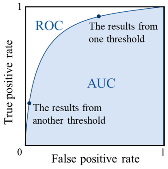
Figure 4.
Receiver operating characteristic (ROC) curve and the calculation of the area under curve (AUC) value.
4. Results
4.1. The Performance of the Pheno-Deep Method
4.1.1. The Pheno-Deep Method in Comparison to Deep Learning Alone Method
The performance measures of the pheno-deep method and the deep learning alone method (which is trained with field collected samples) are shown in Table 2. The mean overall accuracy of the pheno-deep method is 88.8%, only 2.4% lower than the deep learning alone method. The mean AUC value of the pheno-deep method is 94.4%, only 1.3% lower than that of the deep learning alone method. The mean precision and recall scores of the pheno-deep method are also close to that of the deep learning alone method. The difference between precision and recall scores of the pheno-deep method are slightly bigger than that of the deep learning alone method. All measure scores suggest that the pheno-deep method achieved a very close performance to that of the deep learning alone method which requires field samples for training.
Table 2.
The performance of the pheno-deep method and the deep learning alone method.
A hypothesis test was conducted to assess if the difference of 2.4% in mean overall accuracy is significant between the pheno-deep method and the deep learning alone method. The classification errors were assumed to be independent when validating the overall accuracies using 364 validation samples, therefore the number of correct classification samples should satisfy a binomial distribution. The hypothesis is that the overall accuracy of the pheno-deep method is not different from that of the deep learning alone method. Under this hypothesis, the probability of X number of samples being correctly classified can be applied to a binomial distribution with parameter n being 364 (the total number of samples) and parameter p being 88.8% (the accuracy of the pheno-deep method). The probability with k correctly classified samples can be calculated with
The probability of having 91.2% or more of the validation samples (that is 332 samples or more) correctly classified was calculated as
which is greater than the probability of 0.05 often taken as the default greater than which the significance test fails.
P (X ≥ 332) = B (332; 364, 88.8%) + … + B (364; 364, 88.8%) = 0.0813
Even though the performance measures of the pheno-deep method are not as high as the deep learning alone method, the difference in overall accuracy is not significant. Furthermore, the pheno-deep method does not require field sampling efforts which is a requirement for the deep learning alone method or a cost for the performance stipend gained by the deep learning alone method. In addition, the pheno-deep method allows users to collect a large amount of samples without adding sampling cost. The large samples might improve the performance of the pheno-deep method, which will be discussed in Section 5.1.
4.1.2. The Pheno-Deep Method in Comparison to Phenological Alone Method
The performance measures of the phenological alone method and the pheno-deep method with only EVI2 and LSWI data are shown in Table 3. The mean overall accuracy of the pheno-deep method is 87.2%, 13.0% higher than that of the phenological alone method. Other performance measures also suggest that the pheno-deep method achieved better performance than the phenological alone method. It is also worth noting that the phenological alone method has a precision score that is 17.4% (86.8–69.4%) higher than recall score, indicating the over-prediction of rice paddies. This difference in the pheno-deep method is only 5.8% (90.6–84.8%). Even though the pheno-deep method is trained with samples collected based on the phenological alone method, the over-prediction of rice paddies in the pheno-deep method is not as obvious as the phenological alone method. These results suggest that the pheno-deep method can overcome some of the errors from the phenological alone method, which attests that it is possible to train a deep learning model using samples from the results obtained with a less accurate but easy classifier to improve the final classification.
Table 3.
The performance of the pheno-deep method with only two-band Enhanced Vegetation Index (EVI2) and Land Surface Water Index (LSWI) data and the phenological alone method.
4.2. The Spatial Distributions Maps from the Three Methods
The classification maps, one from the 50 experiments of the pheno-deep and one of the deep learning alone method, as well as the classification map from the phenological alone method are shown in Figure 5 to illustrate the spatial patterns of the predicted rice paddies. The green areas are recognized as rice paddies while the grey areas are identified as non-rice paddy areas. The phenological alone method generally identifies more rice paddy areas than the other methods, caused by the over-prediction of rice paddy areas as indicated in a much higher precision than recall. The map from the pheno-deep method is very similar to that of the deep learning alone method. These two maps identify more rice paddies in the north and less rice paddies in the central and southern area than the phenological alone method. The spatial patterns predicted by the pheno-deep method and the deep learning alone method match the terrain conditions of the area better.
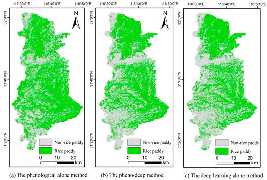
Figure 5.
The rice paddy distribution maps from: (a) the phenological alone method; (b) the pheno-deep method; (c) the deep learning alone method.
As is shown in the topographic map in Figure 3, there are three major terrain areas. The north is mainly occupied by plains where more extensive paddy rice planting is expected. The central and southern areas are dominated by hills and mountains where rice-paddy is not predominant. The overall accuracies of the above three maps were calculated over the areas of three terrain conditions (Table 4). The number of validation samples used in the northern, central, and southern areas are 135, 169, and 60, respectively. The pheno-deep method can better capture the distribution of rice paddy in the north than the other two methods. In the central areas, the accuracy of pheno-deep method is much higher than the phenological method and is slightly lower than that of the deep learning method. All three methods obtained high accuracies in the southern areas while the pheno-deep method did the best among three methods. The pheno-deep method has a better performance identifying rice paddies in the plain and mountainous areas, while the deep learning alone methods identified rice paddies better in the hills and mountains. Overall, the pheno-deep method and the deep learning alone method captures the spatial patterns of rice paddies better.
Table 4.
The overall accuracies (OA) of the three maps within three areas of different terrain conditions.
The computational times for mapping the spatial distribution of the three methods were also recorded during the experiment. It took 13,442 s for the pheno-deep method to produce a rice paddy distribution map, 12,472 s for the deep learning alone method, and 575 s for the phenological alone method. The pheno-deep method took slightly more time than the deep learning alone method and much more than the phenological alone method. It should also be noted that the pheno-deep method does not require any field samples as the deep learning alone method does, and its accuracy improved greatly from the phenological alone method. The additional computing time is not a significant concern in the application of the pheno-deep method.
5. Discussions
5.1. Impacts of the Sample Sizes
The performance of the pheno-deep method was tested with different sample sizes ranging from 100 to 10,000. For each sample size, the experiment was repeated for 50 times as described in Section 3.3. The results are shown in Table 5. As the sample size grows from 100 to 7500, the mean overall accuracy of the pheno-deep method increases while the standard deviation narrows. When the sample size is greater than 7500, the mean overall accuracy of the pheno-deep method rose to 89.8% and the narrowing of standard deviation of overall accuracy becomes very small, even stops. This proves that by enlarging the size of the training samples, the pheno-deep method can be improved with higher mapping accuracy and better stability, and the performance tends to stabilize when the sample size is bigger than 7500. It should be noted that increasing the size of training samples under the pheno-deep does not incur any costs. Therefore, the sample size can be easily enlarged to achieve a better performance.
Table 5.
The impacts of sample size on the performance of the pheno-deep method.
5.2. Impacts of the Sampling Intervals
The quality (representativeness) of the samples from the phenological method depends on their normalized RCLE values. The user-defined intervals, which control where samples were selected, are expected to have impacts on the performance of the pheno-deep method. Here the impacts of the different sampling interval ranges were examined. As stated before, the samples for rice paddy are drawn from one range somewhere between 0.0 and 0.5 and non-rice paddy samples were from another somewhere between 0.5 and 1.0. The ranges for rice paddy were set by shrinking the same amount from 0.0 and from 0.5. For example, the range of 0.20–0.30 was created by increasing 0.2 from 0.0 and decreasing 0.2 from 0.5. The ranges for the non-rice paddy samples were set similarly (Table 6). For each pair of the ranges, 50 sets of samples were selected to examine the pheno-deep method.
Table 6.
The impacts of sampling intervals on sample quality and mapping accuracy.
The accuracies of the training samples (as determined by the accuracy of the areas whose normalized RCLE values falling into the ranges used for selecting the samples) and performances of the pheno-deep method under different interval settings are also shown in Table 6. The overall accuracies (OA) of the training samples increases as the interval range gets narrower. The overall accuracies (OA) of the pheno-deep method range from 86.2% to 88.8% over different interval settings. This suggests that the sampling intervals do not have a substantial impact on the performance of the pheno-deep method, which is contrary to our earlier expectation. Among the different interval settings, the whole ranges (setting 5) performed the worst while the narrow and middle ranges (setting 1 and setting 2) outperformed the other settings. This might be related to that fact that the whole range would contain samples which are either erroneous (samples with normalized RCLE values close to 0.5) or too-pure (samples with normalized RCLE values close to 0.0 or 1.0) while the narrower middle ranges would contain more representative samples. This experiment suggests that a narrower range such as settings 1 and 2 would be preferable for selecting training samples based on the phenological method.
Furthermore, the overall accuracies of the pheno-deep method over all settings are higher than their respective sample accuracies, attesting that the pheno-deep method can overcome the noises in the training samples and obtain a better performance. The idea to train the samples collected based on phenological alone method for a deep learning model can indeed produce results with higher accuracies than the samples used for training.
5.3. Impacts of Learning Models
The LSTM model was selected to be the learning model in the pheno-deep method due to its advantages on processing time series data. To examine if LSTM can outperform other machine learning models, the LSTM component was substituted with other models in the pheno-deep method. For this purpose, random forest [39] (RF) and support vector machine [40] (SVM) were chosen due to their popularity in rice paddy mapping researches [13,14].
The overall accuracies of the pheno-deep method with other two different learning models are shown in Table 7. The mean overall accuracy was 88.8% for the pheno-deep method, and 88.5% for the learning model being RF model and SVM. The mean precision and mean recall with different learning models also came very close. These measures suggest that the performances of these three learning models are about the same. This means that the samples collected based on the phenological method can also be used to train other machine learning models and achieve acceptable results, and that the idea to combine the phenological method and the machine learning methods is plausible in general for rice paddy identification.
Table 7.
The mapping accuracy with different learning models.
6. Conclusions
This paper explored a new means to predict spatial distribution (mapping) of rice paddy using remote sensing data by coupling phenological and deep learning methods. The phenological methods are easy to implement but often with low accuracies. On the other hand, the deep learning methods can produce high accuracy results but require a large number of samples to train the learning model. The work reported in this paper suggests that it is possible and practical to mitigate the above-stated deficiencies by coupling these two types of methods. The phenological approaches can be used to delineate the quantitative phenological measures for generating large training samples. The so-generated samples may not be at the level of accuracy of field samples, but with the use of the deep learning model (even other machine learning models), which are capable of mitigating the noise in the training samples, the negative impacts of the low accuracy of the samples may be minimized. Thus, mapping at an acceptable level of accuracy can be achieved from the deep learning models trained with samples from phenological results. The case study reported in this paper using the pheno-deep method even suggests that the results with much less field sampling efforts are very close to the results that come with high sampling costs, attesting that it is possible in general to combine knowledge-based methods such as phenological methods with data-driven methods such as deep learning methods in the spatial predictions (mapping) of geographic variables using remote sensing data.
Author Contributions
Conceptualization, A.-X.Z.; methodology, A.-X.Z., H.-B.P., and F.-H.Z.; software, F.-H.Z. and H.-B.P.; validation, F.-H.Z. and H.-B.P.; formal analysis, F.-H.Z.; investigation, H.-B.P.; resources, A.-X.Z.; data curation, H.-B.P. and F.-H.Z.; writing—original draft preparation, F.-H.Z.; writing—review and editing, A.-X.Z.; visualization, F.-H.Z.; supervision, A.-X.Z. and J.-Z.L.; project administration, A.-X.Z.; funding acquisition, A.-X.Z. All authors have read and agreed to the published version of the manuscript.
Funding
This research was funded by grants from National Natural Science Foundation of China (Project No.: 41871300, 41431177), PAPD (A Project Funded by the Priority Academic Program Development of Jiangsu Higher Education Institutions), and the China Scholarship Council (Project No.: 201904910630).
Institutional Review Board Statement
Not applicable.
Informed Consent Statement
Not applicable.
Data Availability Statement
The data presented in this study are openly available in “Mapping rice paddy distribution using remote sensing with pheno-deep method in Lu’an, Anhui, China” at doi:10.17605/OSF.IO/76W52.
Acknowledgments
Supports to A-Xing Zhu through the Vilas Associate Award, the Hammel Faculty Fellow Award, and the Manasse Chair Professorship from the University of Wisconsin-Madison are greatly appreciated.
Conflicts of Interest
The authors declare no conflict of interest.
References
- Craufurd, P.Q.; Wheeler, T.R. Climate Change and the Flowering Time of Annual Crops. J. Exp. Bot. 2009, 60, 2529–2539. [Google Scholar] [CrossRef] [PubMed]
- Xiao, X.; Boles, S.; Frolking, S.; Salas, W.; Moore, B.; Li, C.; He, L.; Zhao, R. Observation of Flooding and Rice Transplanting of Paddy Rice Fields at the Site to Landscape Scales in China Using VEGETATION Sensor Data. Int. J. Remote Sens. 2002, 23, 3009–3022. [Google Scholar] [CrossRef]
- Qiu, B.; Li, W.; Tang, Z.; Chen, C.; Qi, W. Mapping Paddy Rice Areas Based on Vegetation Phenology and Surface Moisture Conditions. Ecol. Indic. 2015, 56, 79–86. [Google Scholar] [CrossRef]
- Dong, J.; Xiao, X. Evolution of Regional to Global Paddy Rice Mapping Methods: A Review. ISPRS J. Photogramm. Remote Sens. 2016, 119, 214–227. [Google Scholar] [CrossRef]
- Guo, Y.; Jia, X.; Paull, D.; Benediktsson, J.A. Nomination-Favoured Opinion Pool for Optical-SAR-Synergistic Rice Mapping in Face of Weakened Flooding Signals. ISPRS J. Photogramm. Remote Sens. 2019, 155, 187–205. [Google Scholar] [CrossRef]
- Zhan, P.; Zhu, W.; Li, N. An Automated Rice Mapping Method Based on Flooding Signals in Synthetic Aperture Radar Time Series. Remote Sens. Environ. 2021, 252, 112112. [Google Scholar] [CrossRef]
- Badhwar, G.D.; Gargantini, C.E.; Redondo, F. Landsat Classification of Argentina Summer Crops. Remote Sens. Environ. 1987, 21, 111–117. [Google Scholar] [CrossRef]
- McCloy, K.R.; Smith, F.R.; Robinson, M.R. Monitoring Rice Areas Using LANDSAT MSS Data. Int. J. Remote Sens. 1987, 8, 741–749. [Google Scholar] [CrossRef]
- Fang, H. Rice Crop Area Estimation of an Administrative Division in China Using Remote Sensing Data. Int. J. Remote Sens. 1998, 19, 3411–3419. [Google Scholar] [CrossRef]
- Rao, N.R.; Garg, P.K.; Ghosh, S.K. Development of an Agricultural Crops Spectral Library and Classification of Crops at Cultivar Level Using Hyperspectral Data. Precis. Agric. 2007, 8, 173–185. [Google Scholar] [CrossRef]
- John, J.; Bindu, G.; Srimuruganandam, B.; Wadhwa, A.; Rajan, P. Land Use/Land Cover and Land Surface Temperature Analysis in Wayanad District, India, Using Satellite Imagery. Ann. GIS 2020, 26, 1–18. [Google Scholar] [CrossRef]
- Gumma, M.K. Mapping Rice Areas of South Asia Using MODIS Multitemporal Data. J. Appl. Remote Sens. 2011, 5, 53547. [Google Scholar] [CrossRef]
- Cai, Y.; Lin, H.; Zhang, M. Mapping Paddy Rice by the Object-Based Random Forest Method Using Time Series Sentinel-1/Sentinel-2 Data. Adv. Space Res. 2019, 64, 2233–2244. [Google Scholar] [CrossRef]
- Clauss, K.; Yan, H.; Kuenzer, C. Mapping Paddy Rice in China in 2002, 2005, 2010 and 2014 with MODIS Time Series. Remote Sens. 2016, 8, 434. [Google Scholar] [CrossRef]
- Chen, C.; Mcnairn, H. A Neural Network Integrated Approach for Rice Crop Monitoring. Int. J. Remote Sens. 2006, 27, 1367–1393. [Google Scholar] [CrossRef]
- Wan, L.; Zhang, H.; Lin, G.; Lin, H. A Small-Patched Convolutional Neural Network for Mangrove Mapping at Species Level Using High-Resolution Remote-Sensing Image. Ann. GIS 2019, 55, 45–55. [Google Scholar] [CrossRef]
- Tao, H.; Li, M.; Wang, M.; Lü, G. Genetic Algorithm-Based Method for Forest Type Classification Using Multi-Temporal NDVI from Landsat TM Imagery. Ann. GIS 2019, 25, 33–43. [Google Scholar] [CrossRef]
- Cai, Y.; Guan, K.; Peng, J.; Wang, S.; Seifert, C.; Wardlow, B.; Li, Z. A High-Performance and in-Season Classification System of Field-Level Crop Types Using Time-Series Landsat Data and a Machine Learning Approach. Remote Sens. Environ. 2018, 210, 35–47. [Google Scholar] [CrossRef]
- Rußwurm, M.; Körner, M. Multi-Temporal Land Cover Classification with Long Short-Term Memory Neural Networks. In Proceedings of the International Archives of the Photogrammetry, Remote Sensing and Spatial Information Sciences—ISPRS Archives, Hannover, Germany, 6–9 June 2017; Volume 42, pp. 551–558. [Google Scholar]
- Onojeghuo, A.O.; Blackburn, G.A.; Wang, Q.; Atkinson, P.M.; Kindred, D.; Miao, Y. Mapping Paddy Rice Fields by Applying Machine Learning Algorithms to Multi-Temporal Sentinel-1A and Landsat Data. Int. J. Remote Sens. 2018, 39, 1042–1067. [Google Scholar] [CrossRef]
- Jiang, Z.; Huete, A.; Didan, K.; Miura, T. Development of a Two-Band Enhanced Vegetation Index without a Blue Band. Remote Sens. Environ. 2008, 112, 3833–3845. [Google Scholar] [CrossRef]
- Xiao, X.; Hollinger, D.; Aber, J.; Goltz, M.; Davidson, E.A.; Zhang, Q.; Moore, B. Satellite-Based Modeling of Gross Primary Production in an Evergreen Needleleaf Forest. Remote Sens. Environ. 2004, 89, 519–534. [Google Scholar] [CrossRef]
- Zhu, A.-X. A Similarity Model for Representing Soil Spatial Information. Geoderma 1997, 77, 217–242. [Google Scholar] [CrossRef]
- Zhu, A.X. Measuring Uncertainty in Class Assignment for Natural Resource Maps under Fuzzy Logic. Photogramm. Eng. Remote Sens. 1997, 63, 1195–1201. [Google Scholar]
- Qi, F.; Zhu, A.X. Knowledge Discovery from Soil Maps Using Inductive Learning. Int. J. Geogr. Inf. Sci. 2003, 17, 771–795. [Google Scholar] [CrossRef]
- Zhu, A.-X.; Miao, Y.; Liu, J.; Bai, S.; Zeng, C.; Ma, T.; Hong, H. A Similarity-Based Approach to Sampling Absence Data for Landslide Susceptibility Mapping Using Data-Driven Methods. Catena 2019, 183, 104188. [Google Scholar] [CrossRef]
- Hochreiter, S.; Schmidhuber, J. Long Short-Term Memory. Neural Comput. 1997, 9, 1735–1780. [Google Scholar] [CrossRef]
- Lu’an Statistical Yearbook Committee. Lu’an Statistical Yearbook 2017; China Statistical Press: Beijing, China, 2017. [Google Scholar]
- Atmospheric Correction of a (Single) Sentinel 2 Image. Available online: https://github.com/samsammurphy/gee-atmcorr-S2 (accessed on 1 June 2020).
- Wilson, R.T. Py6S: A Python Interface to the 6S Radiative Transfer Model. Comput. Geosci. 2013, 51, 166–171. [Google Scholar] [CrossRef]
- Eilers, P.H.C. A Perfect Smoother. Anal. Chem. 2003, 75, 3631–3636. [Google Scholar] [CrossRef]
- Tucker, C.J. Red and Photographic Infrared Linear Combinations for Monitoring Vegetation. Remote Sens. Environ. 1979, 8, 127–150. [Google Scholar] [CrossRef]
- Chollet, F. Keras: The Python Deep Learning Library; Astrophysics Source Code Library, 2018. Available online: https://ui.adsabs.harvard.edu/abs/2018ascl.soft06022C/abstract (accessed on 1 April 2021).
- Han, J.; Moraga, C. The Influence of the Sigmoid Function Parameters on the Speed of Backpropagation Learning. In From Natural to Artificial Neural Computation; Mira, J., Sandoval, F., Eds.; Springer: Berlin/Heidelberg, Germany, 1995; Volume 930, pp. 195–201. [Google Scholar] [CrossRef]
- Kingma, D.P.; Ba, J.L. Adam: A Method for Stochastic Optimization. In Proceedings of the 3rd International Conference on Learning Representations, ICLR 2015—Conference Track Proceedings, San Diego, CA, USA, 7–9 May 2015. [Google Scholar]
- Lin, T.Y.; Goyal, P.; Girshick, R.; He, K.; Dollar, P. Focal Loss for Dense Object Detection. IEEE Trans. Pattern Anal. Mach. Intell. 2020, 42, 2980–2988. [Google Scholar] [CrossRef]
- Powers, D.M.W. Evaluation: From Precision, Recall and F-Measure to ROC, Informedness, Markedness and Correlation. J. Mach. Learn. Technol. 2011, 2, 37–63. [Google Scholar]
- Fawcett, T. An Introduction to ROC Analysis. Pattern Recognit. Lett. 2006, 27, 861–874. [Google Scholar] [CrossRef]
- Breiman, L. Random Forests. Mach. Learn. 2001, 45, 5–32. [Google Scholar] [CrossRef]
- Cortes, C.; Vapnik, V. Support-Vector Networks. Mach. Learn. 1995, 20, 273–297. [Google Scholar] [CrossRef]


Publisher’s Note: MDPI stays neutral with regard to jurisdictional claims in published maps and institutional affiliations. |
© 2021 by the authors. Licensee MDPI, Basel, Switzerland. This article is an open access article distributed under the terms and conditions of the Creative Commons Attribution (CC BY) license (https://creativecommons.org/licenses/by/4.0/).