FE-YOLO: A Feature Enhancement Network for Remote Sensing Target Detection

Abstract

In the past few decades, target detection from remote sensing images gained from aircraft or satellites has become one of the hottest topics. However, the existing algorithms are still limited by the detection of small remote sensing targets. Benefiting from the great development of computing power, deep learning has also made great breakthroughs. Due to a large number of small targets and complexity of background, the task of remote sensing target detection is still a challenge. In this work, we establish a series of feature enhancement modules for the network based on YOLO (You Only Look Once) -V3 to improve the performance of feature extraction. Therefore, we term our proposed network as FE-YOLO. In addition, to realize fast detection, the original Darknet-53 was simplified. Experimental results on remote sensing datasets show that our proposed FE-YOLO performs better than other state-of-the-art target detection models.

1. Introduction

The task of target detection includes prediction of location information and category information of the target. It is one of the most important components of many applications, such as pedestrian detection [1,2], defect detection [3,4] and obstacle detection [5,6] in automatic drive. In the research of target detection, remote sensing target detection is one of the key research topics because of its important applications in military applications, such as location and identification of military targets [7], military reconnaissance [8] and military navigation [9]. With the maturity of satellite and aerial photography technology, high quality remote sensing images can be generated. It has far-reaching significance to remote sensing target detection. Remote sensing images usually have lower resolution compared with ordinary images. Due to the special method of acquisition, there are several features of remote sensing images that ordinary images do not have:

(1)

Scale diversity: remote sensing images are taken at altitudes ranging from hundreds of meters to dozens of kilometers. Even with the same target, the scales are quite different. By contrast, the scales of the targets in ordinal images have few differences.

(2)

Particularity of perspective: most remote sensing images are from the top view angle, while ordinary images are usually from horizontal view angle.

(3)

The small size of the targets: remote sensing targets are acquired at high altitude and contain a large number of small targets which may be of large size in ordinary images. For example, in remote sensing images, the pixels of aircraft may be only 10 × 10 to 20 × 20, and for cars may be even less.

(4)

Diversity of directions: the directions of a certain kinds of targets in remote sensing images are often varied, while target direction in the normal image is basically determined.

Due to the particularities of remote sensing targets compared with ordinary targets, remote sensing target detection is still a challenge for researchers.

Before the great development of deep learning technology, the mainstream algorithms of target detection could be divided into three steps: (1) search for the areas where the targets may lie in (region of interest, i.e., ROIs); (2) extract the features of the regions; (3) provide features for the classifier. In order to detect remote sensing targets efficiently, many outstanding algorithms have been proposed. A research group led by Fumio Yamazaki proposed an algorithm based on target motion contour extraction for ‘Quick bird’ remote sensing images and aerial images. A method of region correlation was introduced to find the best matching position in multispectral images by using the vehicle results extracted from panchromatic images. According to the dense distribution of vehicle targets, J. Leitloff et al. adopted Geographic Information System (GIS) information to assist to determine the location and direction of the road and then extracted the areas of interest and the lanes of concern. Then the methods of target contour extraction, shape function filtering and minimum variance optimization were used to extract the vehicles under the state of aggregation. For ship target detection, the Integrated Receiver Decoder (IRD) research group divided the key steps of target detection and recognition into three steps: predetection, feature extraction and selection, classification and decision. It realized the detection of ship targets based on optical remote sensing images. Despite the tireless efforts of researchers, accuracy remains unsatisfactory.

Within the past ten years, the rapid development of deep learning represented by Convolutional Neural Networks (CNNs) [10,11,12] seems to have brought some light to the field of target detection. Region-based CNN (R-CNN) [13] proposed in 2014 was the milestone in target detection based on convolutional neural networks. It treated target detection as a classification problem. Based on R-CNN, a series of improved algorithms, such as Fast R-CNN [14] and Faster R-CNN [15] were proposed subsequently. Since R-CNN was proposed, target detection algorithms based on CNN have developed rapidly.

Generally speaking, we can divide these algorithms into two categories, i.e., one-stage and two-stage. The two-stage ones are represented by the milestone of convolutional neural network, i.e., R-CNN mentioned above. They also contain Fast R-CNN, Faster R-CNN, Mask R-CNN [16], SPP-net [17,18,19], FPN (Feature Pyramid Network) [20,21], R-FCN (Region-based Full Convolutional Network) [22],SNIP [23] and SNIPER [24]. Just as its name implies, the two-stage algorithms first search for regions of interest with the Region Proposed Network (RPN), and then generate category and location information for each proposal. The other ones are one-stage algorithms represented by YOLO series such as YOLO [25], YOLO-V2 [26], YOLO-V3 [27], YOLO-V3 tiny [28] and YOLO-V4 [29], as well as SSD series such as SSD (Single Shot Multibox Detector) [30], DSSD (Deconvolutional Single Shot Multibox Detector) [31], FSSD (Feature Fusion Single Shot Multibox Detector) [32] and LRF [33]. Different from the two-stage algorithms, the one-stage algorithms consider target detection as regression problems directly. The core task of them is to input the image to be detected into the network, and the output layers gain the location and category information of the targets. Both one-stage and two-stage detectors have advantages. Because of the adoption of RPN, the two-stage detectors usually have higher precision, while the advantage of the one-stage detectors is the higher speed.

In the past few decades, a variety of aeronautical and astronautical remote sensing detectors have been developed and used for obtaining information rapidly and efficiently from the ground. The world’s major space powers have accelerated the development of remote sensing technology and successively launched a variety of detection equipment into space. The development of remote sensing technology has greatly improved the shortcomings of traditional ground survey, including small coverage and insufficient data acquisition. As one of the most important tasks of a remote sensing domain, remote sensing target detection is becoming more and more active for researchers. Remote sensing target detection is of great significance to both civilian and military technologies. In the civilian field, high-precision target detection can help cities with traffic management [34] and autonomous driving [35], whereas in the military field, it is widely used in target positioning [36], missile guidance [37] and other aspects.

Compared with superficial machine learning, a Deep Convolutional Neural Network (DCNN) can automatically extract the deeper features of the targets. The use of Deep Convolutional Neural Network for target detection can avoid the process of extracting features of the targets by manually designing specific algorithms according to different targets in superficial machine learning. Therefore, Deep Convolutional Neural Networks have stronger adaptability. Due to the advantages of CNN and the popularity of the target detection algorithms based on CNN, it is the first choice for remote sensing target detection. Unlike conventional images, targets in remote sensing images vary greatly in size. The smaller ones, like aircraft and cars, may take up only 10 × 10 pixels, while the larger ones like playgrounds and overpasses, can take up 300 × 300 pixels. With the difference of imaging devices, light conditions and weather conditions, the remote sensing images are also have a high range of spectral characteristics. For acquisition of increased detecting performance, improvements of network are needed.

Currently, the classical Convolutional Neural Networks have limited performance in detecting remote sensing targets, especially small targets with complex backgrounds. The two-stage detectors usually have lower speed while the one-stage ones are not good at dealing with small targets. Aimed at realizing real-time remote sensing target detection; adapting to remote sensing target detection under different backgrounds, and effectively improving the accuracy of detecting small remote sensing targets, we designed a new one-stage detector named Feature Enhancement YOLO (FE-YOLO). Our proposed FE-YOLO is based on YOLO-V3, which is one of the most popular networks for target detection. The experiments on aerial datasets show that FE-YOLO significantly improves the accuracy of detecting remote sensing targets and reconciles real-time performance simultaneously.

In the rest part of this paper, Section 2 introduces the principle of YOLO series in detail, Section 3 details the improvement strategies of FE-YOLO, Section 5 gives the experimental studies on remote sensing datasets to verify the superiority of our FE-YOLO and Section 5 gives the conclusions of this paper.

2. The Principle of YOLO Series

2.1. The Evolutionary Process of YOLO

The one-stage algorithms represented by YOLO (You Only Look Once) is an end-to-end model based on CNN. Compared with Faster R-CNN, YOLO, it does not have a cockamamie region proposal stage, so it is extremely popular due to its conciseness. YOLO ((a) in Figure 1) was firstly proposed by Joseph Redmon et al. in 2015. When performing target detection, the feature extraction network divides the input image into $S\times S$ grid cells. For each grid, the network predicts $B$ bounding boxes. Each bounding box can gain three predictive values: (1) the probability the target lies in the grid; (2) the coordinates of the bounding box and (3) the category of the target and its probability. For each grid cell, the predictive values include five parameters:$(x,y,w,h,cs)$. Among them, $x$, $y$, $w$, $h$ represent the coordinate, height and width of the central point of the bounding box; $cs$ represents the confidence score of the bounding box. The confidence of the bounding box is defined as: $\mathrm{P}(Object)\times IO{U}_{pred}^{truth}$. If the center of the target lies in the grid, then $\mathrm{P}(Object)=1$, Otherwise, $\mathrm{P}(Object)=0$. The network predicts $C$ classes. Ultimately, the tensor size of the output of the network is: $S\times S\times (B\times 5+C)$. The class-specific confidence can be expressed in Equation (1):

$$\mathrm{P}(Clas{s}_i|Object)\times \mathrm{P}(Object)\times IO{U}_{pred}^{truth}=\mathrm{P}(Class)\times IO{U}_{pred}^{truth}$$

(1)

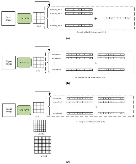
Figure 1. The comparison of YOLO-V1 (you-only-look-once V1) to YOLO-V3.

YOLO-V1 has stunning detecting speed compared to Faster R-CNN. However, its accuracy is lower than other one-stage detectors such as SSD. In addition, for each grid cell, only one target can be detected. To improve the deficiencies of YOLO-V1, in 2017 the advanced version of YOLO (i.e., YOLO-V2) was proposed. YOLO-V2 (in Figure 1b) offered several improvements over the first version. Firstly, instead of FC (Full Connected Layer), YOLO-V2 adopted FCN (Full Convolutional Layers). The feature extraction network was updated to Darknet19. Secondly, utilizing the ideal of Faster R-CNN, YOLO-V2 introduced the concept of anchor box to match the targets of different shapes and sizes. Moreover, Batch Normalization was also adopted. The accuracy of YOLO-V2 was drastically improved compared to YOLO-V1.

In order to improve the accuracy and enhance the performance of detecting multi-scale targets, the most classic YOLO-V3 (in Figure 1c) came on the stage. Different from YOLO-V1 and YOLO-V2, which only have one detection layer, YOLO-V3 sets three different scales. This was inspired from a FPN (Feature Pyramid Network), and the improvement strategy can detect smaller targets. The structure of original YOLO-V3 and Darknet53 are illustrated in Figure 2 and Table 1, respectively.

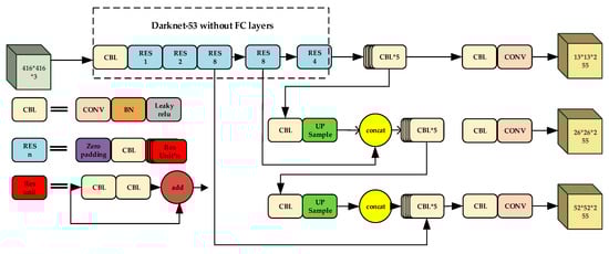
Figure 2. The structure of YOLO-V3.

Table 1. The structure of Darknet53 (input size = 416 × 416).

	Layer	Filter	Size	Output
	Convolutional	32	3 × 3	416 × 416 × 32
	Convolutional	64	3 × 3/2	208 × 208 × 64
	Convolutional	32	1 × 1
1×	Convolutional	64	3 × 3
	Residual			208 × 208 × 64
	Convolutional	128	3 × 3/2	104 × 104 × 128
2×	Convolutional	64	1 × 1
	Convolutional	128	3 × 3
	Residual			104 × 104 × 128
	Convolutional	256	3 × 3/2	52 × 52 × 256
8×	Convolutional	128	1 × 1
	Convolutional	256	3 × 3
	Residual			52 × 52 × 256
	Convolutional	512	3 × 3/2	26 × 26 × 512
8×	Convolutional	256	1 × 1
	Convolutional	512	3 × 3
	Residual			26 × 26 × 512
	Convolutional	1024	3 × 3/2	13 × 13 × 1024
4×	Convolutional	512	1 × 1
	Convolutional	1024	3 × 3
	Residual			13 × 13 × 1024

The loss function of YOLO-V3 can be divided into three parts: (1) coordinate prediction error, (2) IOU (Intersection over Union) error and (3) classification error:

Coordinate prediction error indicates the accuracy of the position of the bounding box, and is defined as:

$$\begin{array}{ll}Erro{r}_{coord}& ={\lambda }_{coord}{\displaystyle {\sum }_{i=1}^{s^2}{\displaystyle {\sum }_{j=1}^B{I}_{ij}^{obj}[{(x_i-{\overline{x}}_i)}^2+{(y_i-{\overline{y}}_i)}^2]}}\\ & +{\lambda }_{coord}{\displaystyle {\sum }_{i=1}^{s^2}{\displaystyle {\sum }_{j=1}^B{I}_{ij}^{obj}[{(w_i-{\overline{w}}_i)}^2+{(h_i-{\overline{h}}_i)}^2]}}\end{array}$$

(2)

In Equation (2), ${\lambda }_{coord}$ refers to the weight of the coordinate error and we select ${\lambda }_{coord}=5$ in this work. $S^2$ is the number of the grid cells of each detection layer while $B$ is the number of the bounding boxes in each grid cell. $I_{ij}^{obj}$ indicates if a target lies in the $j\text{-}\mathrm{th}$ bounding box of the $j\text{-}\mathrm{th}$ grid cell. $x_i,y_i,w_i,h_i$ indicate the abscissa, ordinate, width and height of the center of the ground truth, while ${\overline{x}}_i,{\overline{y}}_i,{\overline{w}}_i,{\overline{h}}_i$ indicate the predicted box.

Intersection over Union (IOU) error indicates the degree of overlap between the ground truth and the predicted box. It can be defined in Equation (3):

$$\begin{array}{ll}Erro{r}_{IOU}& ={\displaystyle {\sum }_{i=1}^{S^2}{\displaystyle {\sum }_{j=1}^B{I}_{ij}^{obj}(C_i-{\overline{C}}_i)}}\\ & +{\lambda }_{noobj}{\displaystyle {\sum }_{i=1}^{S^2}{\displaystyle {\sum }_{j=1}^B{I}_{ij}^{noobj}(C_i-{\overline{C}}_i)}}\end{array}$$

(3)

In Equation (3), ${\lambda }_{noobj}$ refers to the confidence penalty when there is no object; we selected ${\lambda }_{noobj}=0.5$ in this work. $C_i$ and ${\overline{C}}_i$ represent the confidence of the truth and prediction, respectively.

Classification error represents the accuracy of classification and is defined as:

$$Erro{r}_{cls}={\displaystyle {\sum }_{i=1}^{S^2}{\displaystyle {\sum }_{j=1}^B{I}_{ij}^{obj}{\displaystyle {\sum }_{c\in classes}(p_i(c)-{\overline{p}}_i(c))}}}{}^2$$

(4)

In Equation (4), $c$ refers to the class the detected target belongs to. $p_i(c)$ refers to the true probability the target belongs to class $c$.${\overline{p}}_i(c)$ refers to the predicted probability the target belongs to class $c$.

So, the loss function of YOLO-V3 is shown as follows:

$$\begin{array}{ll}Loss& =Erro{r}_{coord}+Erro{r}_{IOU}+Erro{r}_{cls}\\ & ={\lambda }_{coord}{\displaystyle {\sum }_{i=1}^{s^2}{\displaystyle {\sum }_{j=1}^B[{(x_i-{\overline{x}}_i)}^2+{(y_i-{\overline{y}}_i)}^2]}}\\ & +{\lambda }_{coord}{\displaystyle {\sum }_{i=1}^{s^2}{\displaystyle {\sum }_{j=1}^B[{(w_i-{\overline{w}}_i)}^2+{(h_i-{\overline{h}}_i)}^2]}}\\ & +{\displaystyle {\sum }_{i=1}^{S^2}{\displaystyle {\sum }_{j=1}^B{I}_{ij}^{obj}(C_i-{\overline{C}}_i)}}\\ & +{\lambda }_{noobj}{\displaystyle {\sum }_{i=1}^{S^2}{\displaystyle {\sum }_{j=1}^B{I}_{ij}^{obj}(C_i-{\overline{C}}_i)}}\\ & +{\displaystyle {\sum }_{i=1}^{S^2}{\displaystyle {\sum }_{j=1}^B{I}_{ij}^{obj}{\displaystyle {\sum }_{c\in classes}(p_i(c)-{\overline{p}}_i(c))}}}{}^2\end{array}$$

(5)

2.2. K-Means for Appropriate Anchor Boxes

The concept of an anchor box was firstly proposed in Faster-RCNN. An anchor box is used to assist the network with appropriate bounding boxes. Illuminated by Faster-RCNN, YOLO introduced the ideal of an anchor box after YOLO-V2 was proposed. The core ideal of an anchor box is to make the bounding boxes match the size of targets before detection. Compared with Faster-RCNN, YOLO-V3 runs K-means to gain appropriate anchor boxes instead of doing it manually. In order to acquire optimal sizes of anchor boxes, they ought to be as approximate as possible compared with the ground truth of the targets. So, the IOU (the intersection over union) values of them must be as large as possible. For each ground truth of the targets: $g{t}_j(x_j,y_j,w_j,h_j),j\in \{1,\dots ,N\}$, $(x_j,y_j)$ refer to the center of the target and $(w_j,h_j)$ refer to the width and height of it. Otherwise, we give the concept of distance. The distance between ground truth and bounding box can be expressed as:

$$d(box-centroid)=1-IOU(box,centroid)$$

(6)

$IOU$ between them is defined as follows:

$$IOU=\frac{S_{overlop}}{S_{union}}$$

(7)

$S_{ocerlap}$ refers to the overlap area between the predicted box and ground truth, while $S_{union}$ refers to the union area between them.

The larger the $IOU$, the larger the distance and the smaller the distance between the ground truth and the bounding box. Table 2 gives the pseudo code of K-means:

Table 2. Pseudo code of K-means for anchor boxes.

The K-Means Clustering for Anchor Boxes
1: Set $k$ random cluster center points randomly: $(W_i,H_i),i\in \{1,\dots ,k\}$. $W_i,H_i$ refers to the width and height of each anchor box. The width and height are both proportional relative to the whole image.
2: Calculate the distance between each ground truth and each cluster center (bounding box). Since the position of anchor box is not fixed, the center point of each ground truth is coincident with the clustering center.

When detecting targets, we need to get the values of bounding boxes based on predicted values. The process is shown in Equation (8). In Equation (8), $t_x,t_y,t_w,t_h$ refer to the predicted values of the network. $c_x,c_y$ refer to the offset relative to the upper left. In addition, the correspondence between the bounding box and the output values is shown in Figure 3.

$$\begin{array}{l}{b}_x=\sigma (t_x)+c_x\\ b_y=\sigma (t_y)+c_y\\ b_w=p_x+e^{t_w}\\ b_h=p_h+e^{t_h}\\ c_x=1/(1+e^{-x})\end{array}$$

(8)

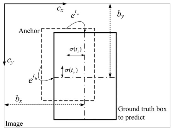
Figure 3. The decoding schematic.

2.3. NMS for Eliminating Superfluous Bounding Boxes

After the process of decoding, the network may acquire a series of bounding boxes. Among them, there are going to be several bounding boxes correspond to one target. To eliminate superfluous bounding boxes and retain the most precise boxes, NMS is adopted. NMS consists mainly of three steps:

(1)

Step 1: for the bounding boxes corresponding to each category, we compare the $IOU$ between each bounding box with others.

(2)

Step 2: if the $IOU$s are larger than the threshold we set, then they are considered to correspond to the same target and the bounding box with the higher confidence can be retained. In this work, we set a fixed $IOU$ = 0.5.

(3)

Step 3: repeat step 1 and step 2 until all the boxes are retained.

Algorithm 1 gives the pseudo code of NMS in this paper:

Algorithm 1. The pseudo code of Non-Maximum Suppression (NMS), NMS Algorithm for Our Approach.

Original Bounding Boxes:

$B=[b_1,\dots ,b_s],C=[c_1,\dots ,c_s],threshold=0.6$

B refers to the list of the bounding boxes generated by the network.

C refers to the list of the confidences corresponding to the bounding boxes in C

Detection result:

F refers to the list of the final bounding boxes.

1:  F ← []

2:  while B ≠ [] do:

3:    k ← arg max c

4:    F ← F.append(bk); B ← delB[bk]; C ← del[bk]

5:   for bi ∈ B do:

6:     if IOU(bi, bi) ≥ thresold

7:       B ← delB[bk]; C ← del[bk]

8:     end

9:    end

10: end

3. Related Work

The improved models based on YOLO-V3 mentioned in Section 2 performed poorly in accuracy or real-time performance. Even more insufficient, when facing the remote sensing images with a large amount of small or densely distributed targets, their performance was unsatisfactory. There is still large possibility of improvement for YOLO-V3 model. Our approach aims to achieve three objectives: (1) detect small targets more effectively than other state-of-the-art one-stage detectors; (2) detect densely distributed targets perfectly and (3) realize real-time performance. To achieve the above three purposes, our improvements are shown as follows.

3.1. The Lightweight Feature Extraction Network

YOLO-V3 employs Darknet53 which deepens the network and is appealing due to its speed. However, it is limited by its accuracy, which presents a new problem. For the input image with the size of 416 × 416, the size of the three detection layers was 52, 26, and 13, respectively. In other words, the feature maps of the three detection layers were down-sampled by 32×, 16×, and 8×, respectively. That is to say, if the size of the target is less than 8 × 8, the feature map of it may take up less than one pixel after being processed by the feature extraction network. As a result, the small target is hard to be detected. Otherwise, if the distance of the center of two targets is less than eight pixels, the feature maps of them must lie in the same grid cell, which makes it impossible for the network to distinguish between the two targets. The ability of YOLO-V3 is significant for detecting small targets, but it cannot satisfy the need for detecting small remote sensing targets. Due to vast computing redundancy and the demand of detecting small targets, we adopted two improvements to the feature extraction network. First, we simplified the feature extraction network to some extent by wiping off several residual blocks. Second, we replaced the bottom detection layer with a finer one. These improvements allowed the network to detect the targets with even smaller size. In addition, some densely distributed targets could be better to be differentiate. The structures of residual unit and simplified feature extraction network are shown in Figure 4 and Figure 5, respectively.

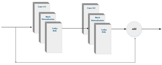
Figure 4. The structure of residual unit.

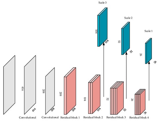
Figure 5. The structure of feature extraction network.

3.2. Feature Enhancement Modules for Feature Extraction Network

The proposed feature extraction network simplifies the calculation tremendously but, at the same time, the property of the network for feature extraction is greatly limited. Many ways can be adopted in improving the performance of the network, such as hardware upgrades and larger scale of datasets. When objective conditions are limited, the most direct way to improve the performance is to increase depth or width of the network. The depth refers to the number of layers of the network. The width refers to the number of the channels per layer. However, this way may lead to two problems:

(1)

With the increase of depth and width, the parameters of the network are greatly increased, which may easily result in overfitting.

(2)

Increasing the size of the network results in an increase in computation time.

In order to solve the problem of overfitting, we focused on the skip connection which has been widely used in Deep Convolutional Neural Network. During the process of forward propagation, skip connection enable a very top layer to obtain information from the bottom layer. On the other hand, during the process of backward propagation, it facilitates gradient back-propagation to the bottom layer without diminishing magnitude, which effectively alleviates gradient vanishing problem and eases the optimization. ResNet is one of the first network which adopt skip connection.

Darknet53 in YOLO-V3 employs ResNet [38] which consist of several residual units (see in Figure 4). Nevertheless, too many residual units lead to computation redundancy, while the performance of lightweight feature extraction network is limited. For this purpose, we needed to specifically design feature enhancement modules.

ResNet, which was employed in the feature extraction network of YOLO-V3 (i.e., Darknet53), deepens the network and avoids gradient fading simultaneously. It adds input to the output of the convolutional layers directly (in Figure 3). The output of it can be expressed in Equation (9):

$$r^k=r^{k-1}+G(r^{k-1})$$

(9)

In Equation (9), $r^k$ refers to the $k\text{-}\mathrm{th}$ residual unit of the network and $G(.)$ refers to the transfer function (i.e., Conv (1 × 1)-BN-ReLU-Conv (3 × 3)-BN-ReLU modules in Figure 3).

In 2017, another classic network i.e., DenseNet [39], was proposed by Huang et al. Different from ResNet, DenseNet concatenates the output of each layer onto the input of each subsequence layer. Although the width of the densely connected network increases linearly with depth, DenseNet provides higher parameter efficiency than ResNet. The output of each layer can be expressed in Equation (10):

$$h^l=x^l=F_l[x_0,x_1,\dots ,x_{l-1}]$$

(10)

In Equation (10), $h^l$ refers to the output of DenseNet, $x^l$ refers to the feature map of $l\text{-}\mathrm{th}$ layer and $F_l$ refers to the transfer function. There are $l(l+1)/2$ connections in the network. The architecture comparison of them is exhibited in Figure 6.

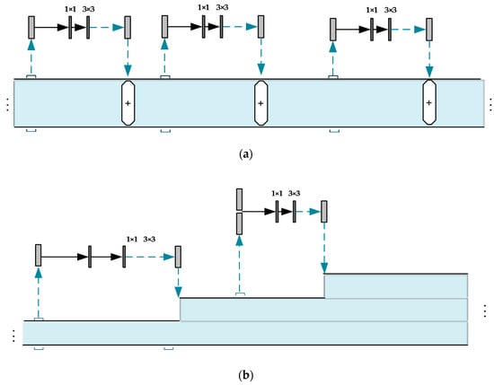
Figure 6. The architecture comparison of. (a) ResNet. (b) DenseNet.

From the architecture comparison in Figure 6 with Equations (9) and (10), we can see ResNet reuses the feature that the previous layers have extracted. The real features extracted by convolutional layer are much more purer. They are basically new features that have not been extracted before. So, the redundancy of features extracted by ResNet is lower. By contrast, the features extracted by previous layers are no longer simply reused by the later layers in DenseNet but create entirely new features. The features extracted in the later layer of this structure are likely to be those extracted by the previous layer. Combining the above analysis, ResNet has a higher reuse rate but lower redundancy rate of features. DenseNet creates new features but has a higher redundancy rate. Based on the characteristics of the above network, combining these structures and the network has even more power. So, DPN came into being. Dual Path Network (DPN) was proposed by Chen et al. DPN is a strong network with the incorporation of ResNet and DenseNet. The architecture is shown in Figure 7.

Figure 7. Dual Path architecture.

For each unit in DPN, the layer that goes through the convolution is divided into two parts (see Structure 1 and Structure 2 in Figure 6). The two parts can be served as inputs of ResNet and DenseNet, respectively. Then, DPN concatenates the outputs of the two networks as the input of the next unit. By combining the core ideas of the two networks, DPN allows the model to make better use of features. Illuminated by DPN, we made improvements on original feature extraction network (see in Figure 4) by adding two feature enhancement modules after the structure of ‘Residual block 2′ and ‘Residual block 3′, respectively. The feature enhancement modules refer to the principles of DPN, so we called them Dual Path Feature Enhancement Modules (DPFE). The structures of them are shown in Figure 8.

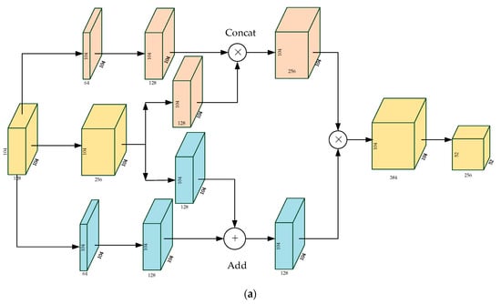
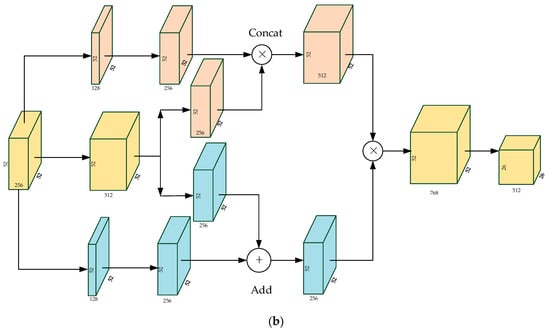
Figure 8. The structures of Dual Path Feature Enhancement Modules (DPFE). (a) DPFE 1. (b) DPFE 2.

3.3. Feature Enhancement Modules for Detection Layers

In YOLO-V3, six convolutional layers are appended to each detection layer. In the entire operation of YOLO-V3, the convolutional layers of three detection layers create a lot of computational redundancy. In addition, many convolutional layers may cause gradient fading. In order to solve this problem, another kind of feature enhancement module was proposed in the detection layers. Inspired by the structures of Inception and ResNet, our proposed feature extraction modules were called Inception and ResNet Feature Enhancement Modules (IRFE). The structures of them are shown in Figure 9.

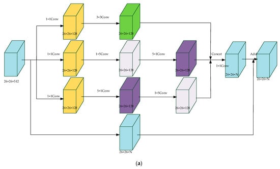
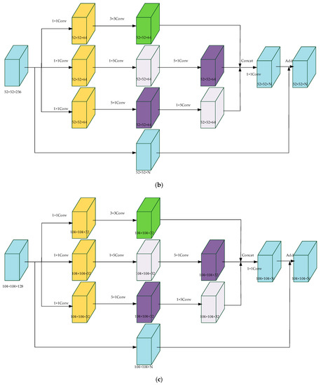
Figure 9. The structures of ResNet Feature Enhancement Modules (IRFE). (a) IRFE1 for Scale 1. (b) IRFE2 for Scale 2. (c) IRFE3 for Scale 3.

In Figure 9, the modules adopt 1 × 1, 3 × 3, 5 × 5 kernels and obtain different sizes of receptive fields. We merged the features to realize fusion of features of different scales. As the network deepens, the features become more abstract and the receptive field involved in each feature is larger. In addition, 1 × 1, 3 × 3, 5 × 5 kernels enable the network to learn more nonlinear relations. At the same times, the combination of residual network enables the network to capture more characteristic information. In order to save time consumed by the module, 3 × 3, 5 × five kernels were decomposed into 1 × 3, 3 × 1 and 1 × 5, 5 × 1 kernels.

Different from convolutional layers in the detection layers of YOLO-V3, our proposed IRFE modules improved the performance of the network by increasing its breadth. In each branch of IRFE, we adopted convolutional kernels of different sizes to gain different receptive fields. We concentrated each branch to enrich the information of each layer.

3.4. The New Residual Blocks Based on Res2Net for Feature Extraction Network

YOLO-V3 relies heavily on a Residual Network (ResNet) in its feature extraction network and achieves good performance. However, it still represents features by the way of hierarchical multiscale representation, which makes the use of inner features of the monolayer inadequate. At present, most of the existing feature extraction methods represent multi-scale features in a hierarchical way. That means either multiscale convolutional kernels are adopted to extract features for each layer (such as SPPNet), or features are extracted for each layer to be fused (such as FPN). In 2019, a new way of connection for residual unit was proposed by Gao et al. and the new improved network was termed as Res2Net. In this method, several small residual blocks are added into the original residual unit. The essence of Res2Net is to construct hierarchical residual connections within a single residual unit. Compared with ResNet, it represents multiscale features by the way of a granular level and can increase the range of receptive fields for each layer. Utilizing the ideal of Res2Net, we proposed ‘Res2 Unit’ for our feature extraction network. Figure 10 shows the structure of our proposed ‘Res2 unit’ and ‘Res2 block’ is made up of several ‘Res2 units’.

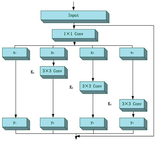
Figure 10. The structure of ‘Res2 unit’.

In each ‘Res2 unit’, the input feature maps are divided into $N$ sub-feature maps (we select n = 4 in this paper) on average. Each subfeature map is represented as $x_i(i=1,2,3,4)$. Compared with the feature maps of ResNet, each sub-feature map is of the same size, but contains only $1/S$ number of channels. $k_i()$ refers to the $3\times 3$ convolutional layer while $y_i$ represents the output of $k_i()$. $y_i$ and can be represented as:

$$y_i=\{\begin{array}{l}{x}_i\hspace{1em}\hspace{1em}\hspace{1em}\hspace{1em}\hspace{1em}\hspace{1em}i=1;\hfill \\ k_i(x_i)\hspace{1em}\hspace{1em}\hspace{1em}\hspace{1em}\hspace{1em}i=2;\hfill \\ k_i(x_i+y_i)\hspace{1em}\hspace{1em}\hspace{1em}2\le i\le N.\hfill \end{array}$$

(11)

In this paper, $y_1$, $y_2$, $y_3$, $y_4$ can be represented as ($\ast$ refers to convolution):

$$\{\begin{array}{l}{y}_1=x_1\hfill \\ y_2=x_2\ast (3\times 3\mathrm{Conv})\hfill \\ y_3=(x_3+x_2\ast (3\times 3\mathrm{Conv}))\ast (3\times 3\mathrm{Conv})\hfill \\ y_4=(x_4+(x_3+x_2\ast (3\times 3\mathrm{Conv}))\ast (3\times 3\mathrm{Conv}))\ast (3\times 3\mathrm{Conv})\hfill \end{array}$$

(12)

In this paper, we set $N$ as the controlling parameter, which refers to the number of input channels that can be divided into multiple feature channels on average. The larger $N$, the stronger the multiscale capability. In this way, we get output of different sizes of receptive fields.

Compared with residual unit, the improved ‘Res2 unit’ makes better use of contextual information and can help the classifier detect small targets, and the targets subject to environmental interference, more easily. In addition, the extraction of features at multiple scales enhances the semantic representation of the network.

3.5. Our Proposed Model

From what has been discussed in Section 4.3 and Section 4.4, our proposed FE-YOLO introduced the lightweight feature extraction network and feature enhancement modules (DPFE and IRFE), Res2Net. The structure of FE-YOLO is shown in Figure 11.

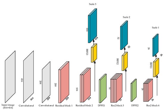
Figure 11. The structure of FE-YOLO.

From the whole network view, the structure of our proposed FE-YOLO is relatively concise. Compared with YOLO-V3, the number of residual blocks of FE-YOLO was drastically reduced. In addition to that, the size of the detection layers was changed from 13 × 13, 26 × 26 and 52 × 52 to 26 × 26, 52 × 52 and 104 × 104, respectively. Besides the lightweight of the feature extraction network, FE-YOLO introduced ‘Res2 blocks’ and replaced the last two residual blocks to increase the range of receptive fields. In addition, feature enhancement modules were adopted to the network for better feature extraction. To show internal structures more clearly, we compared the feature extraction network’s parameters of YOLO-V3 and our FE-YOLO. We exhibit them in Table 3 and Table 4, respectively.

Table 3. The feature extraction network’s parameters of original YOLO-V3.

YOLO-V3
	Conv (3 × 3 × 32)-BN-ReLU	Convolutional
	Conv (3 × 3/2 × 64)-BN-ReLU	Convolutional
RES × 1	Conv (1 × 1 × 32)-BN-ReLU-Conv (3 × 3 × 64)-BN-ReLU	Residual
	Conv (3 × 3/2 × 128)-BN-ReLU	Convolutional
RES × 2	Conv (1 × 1 × 64)-BN-ReLU-Conv (3 × 3 × 128)-BN- ReLU	Residual
	Conv (3 × 3/2 × 256)-BN-ReLU	Convolutional
RES × 8	Conv (1 × 1 × 128)-BN-ReLU-Conv (3 × 3 × 256)-BN- ReLU	Residual
	Conv (3 × 3/2 × 512)-BN- ReLU	Convolutional
RES × 8	Conv (1 × 1 × 256)-BN-ReLU-Conv (3 × 3/ × 512)-BN- ReLU	Residual
	Conv (3 × 3/2 × 1024)-BN-ReLU	Convolutional
RES × 4	Conv (1 × 1 × 512)-BN-ReLU-Conv (3 × 3 × 1024)-BN- ReLU	Residual

Table 4. The feature extraction network’s parameters of FE-YOLO.

MRFF-YOLO
	Conv (3 × 3 × 32)-BN-ReLU	Convolutional
	Conv (3 × 3/2 × 64)-BN-ReLU	Convolutional
RES × 1 (Residual block 1)	Conv (1 × 1 × 32)-BN-ReLU-Conv (3 × 3 × 64)-BN-ReLU	Residual
	Conv (3 × 3/2 × 128)-BN-ReLU	Convolutional
RES × 2 (Residual block 2)	Conv (1 × 1 × 64)-BN-ReLU-Conv (3 × 3 × 128)-BN- ReLU	Residual
DPFE1
RES2 × 4 (Res2 block 3)	Conv (1 × 1 × 128)-BN-ReLU	Residual
	$x_1$	Concat
	$x_2$: Conv (3 × 3 × 64)-BN-ReLU
	$x_3$: Conv (3 × 3 × 64)-BN-ReLU
	$x_4$: Conv (3 × 3 × 64)-BN-ReLU
DPFE2
RES2 × 4 (Res2 block 4)	Conv (1 × 1 × 256)-BN-ReLU	Residual
	$x_1$	Concat
	$x_2$: Conv (3 × 3 × 128)-BN-ReLU
	$x_3$: Conv (3 × 3 × 128)-BN-ReLU
	$x_4$: Conv (3 × 3 × 128)-BN-ReLU

Compared with the ‘residual block’, the number of parameters of the ‘Res2 block’ was not increased. Although our proposed FE-YOLO is not deeper than YOLO-V3, it adopts feature enhancement modules and multireceptive field blocks. In addition, the lightweight feature extraction network makes it more efficient to detect small targets. The superiority of our approach is described in Section 5.

4. Experiments and Results

In this section, we conduct a series of experiments on remote sensing datasets and compared our approach with other state-of-the-art detectors to verify the validity of our approach. MS COCO, RSOD, UCS-AOD and VEDAI datasets are chosen to our contrast experiments. The environment of our experiments is shown as follows: Framework: Python3.6.5, tensorflow-GPU1.13.1. Operating system: Windows 10. CPU: i7-7700k. GPU: NVIDIA GeForce RTX 2070. 50,000 training steps were set. The learning rate of our approach decreased from 0.001 to 0.0001 after 30,000 steps and to 0.00001 after 40,000 steps. The initialization parameters are displayed in Table 5.

Table 5. The initialization parameters of training.

Input Size	Batch Size	Momentum	Learning Rate	Training Step
416 × 416	8	0.9	0.001–0.00001	50,000

4.1. Dataset

The datasets we chose are all labelled by professional team tasks. The MS COCO dataset is a kind of conventional target dataset obtained by Microsoft. The RSOD [40] dataset is issued by Wuhan University in 2015. It contains targets of four categories including aircraft, oil tanks, overpasses and playgrounds. The UCS-AOD [41] dataset is issued by University of Chinese Academy of Sciences in 2015. It contains targets of two categories including aircraft and vehicles. The VEDIA [42] dataset is mainly used for the detection of small vehicles in a variety of environments. The statistics of the three of the above remote sensing target datasets are shown in Figure 12:

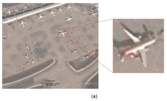
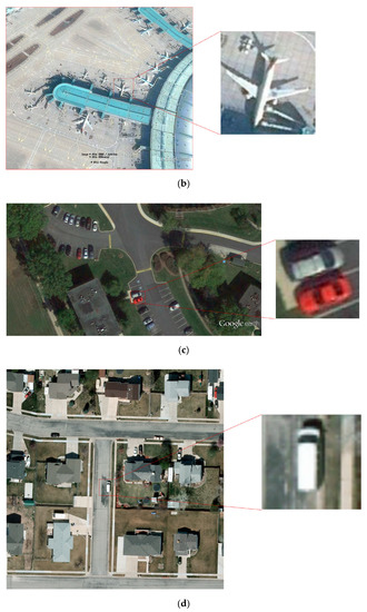
Figure 12. The samples of the datasets.

Figure 12 shows some samples of the datasets we choose. The targets in these samples were under different conditions, such as strong light condition, weak light condition and complex background condition.

4.2. The Sizes of Anchor Boxes for Remote Sensing Datasets

The more cluster center points we set, the larger IOU there was between the ground truth and the anchor boxes. Figure 13 exhibits the variation trend of average IOU as the cluster points increased. We can see that the curves get more and more flat. There are three detection layers in our approach and three anchor boxes were assigned to each detection lay. Table 6 shows the sizes of the anchor boxes of three datasets.

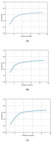
Figure 13. The relationship between number of clusters and average insertion over union (IOU) by K-means clustering, (a) The curve of RSOD dataset, (b) The curve of UCS-AOD dataset, (c) The curve of VEDIA dataset.

Table 6. The sizes of anchor boxes for RSOD, UCS-AOD, and VEDIA dataset.

Dataset		RSOD	UCS-AOD	VEDIA
Anchor	Scale 1	(312,258), (258,218), (241,205)	(296,254), (265,207), (187,158)	(214,201), (189,175), (156,142)
	Scale 2	(188,162), (174,156), (159,124)	(195,172), (181,153), (144,119)	(172,158), (163,142), (154,125)
	Scale 3	(48,36), (41,39), (33,25)	(48,36), (41,39), (33,25)	(35,31), (28,21), (21,13)

4.3. Evaluation Indicators

In order to evaluate the performance of classification models, four classification results are given. The confusion matrix is shown in Table 7:

Table 7. The confusion matrix.

Actual	Predicted	Confusion Matrix
Positive	Positive	TP
Negative	Positive	FP
Positive	Negative	FN
Negative	Negative	TN

In Table 7, TP (True Positive) refers to a sample which is positive in actuality and is positive in prediction, FP (False Positive) denotes a sample that is negative in actuality but is positive in prediction; FN (False Negative) denotes a sample that is positive in actuality but is negative in prediction and TN (True Negative) denotes a sample that is negative in actuality and is negative in prediction.

A single adoption of precision or recall is one-sided. Precision and recall are two indicators that check and balance each other. The tradeoff between them is hard. With the aim of measuring the precision of detecting targets with different categories, AP and mAP were introduced, which are the most important evaluation indicators of target detection.

In addition, Frames per Second (FPS) is also an important indicator for target detection for measuring real-time performance. It refers to the number of frames processed by the target detection algorithm in one second.

4.4. Experimental Process and Index Comparison

4.4.1. Comparative Analysis

In this section, mAP and FPS are adopted to evaluate the performance of target detection models. In order to verify the universality of the performance of our approach, we compared EF-YOLO with the state-of-the-art networks on MS COCO dataset. The experimental results are shown in Table 8.

Table 8. The Comparison of speed and accuracy on MS COCO dataset (test-dev 2017).

Method	Backbone	APS	APM	APL	FPS
SSD	VGG-16	6.14	24.85	40.52	25.2
YOLO-V3	Darknet-53	10.62	29.36	42.17	32.5
YOLO-V4	CSPDarknet-53	19.72	42.58	55.63	30.6
PP-YOLO	ResNet50-vd	19.76	41.89	54.92	68.5
YOLO-V3-SPP	Darknet-53	19.52	35.13	45.52	27.5
FE-YOLO	(Figure 11)	20.83	42.69	55.87	67.4

Table 8 shows the superior performance of our approach on the MS COCO dataset. Even compared with the latest YOLO-V4 and PP-YOLO, our approach still had a little advantage.

Since our approach is devoted to detecting targets in remote sensing images, the experiments ought to be carried out in remote sensing datasets. To verify the superiority of our approach in detecting remote sensing targets, we compared the experimental results of our approach (FE-YOLO) with other state-of-the-art detectors. The comparative results of experiment on RSOD dataset are shown in Table 8.

The experimental results in Table 9 verify the superiority performance of our proposed FE-YOLO. The mAP of FE-YOLO in detecting remote sensing targets on the RSOD dataset was 88.83%. Compared with the original YOLO-V3, it increased by 11.73%. In addition, in comparison to the improved versions of YOLO-V3, our approach was no less impressive. The mAP increased by 11.04% and 12.25%, respectively. Especially, the increase in accuracy of detecting small targets like aircraft and oil tanks was even more pronounced. While maintaining accuracy, the detection speed has been greatly improved compared to YOLO-V3. FPS was up to 65.4, which is close to YOLO-V3. In terms of leak detection rate, FE-YOLO was significantly lower than other state-of-the-art detectors. The comparative results in Table 9 indicate the excellent performance of our approach.

Table 9. The comparative results of different categories in the RSOD dataset.

Method	Backbone	AP (%)					FPS	Leak Detection Rate (%)
		Aircraft	Oil Tank	Overpass	Playground	mAP (IOU = 0.5)
Faster RCNN	VGG-16	85.85	86.67	88.15	90.35	87.76	6.7	11.8
SSD	VGG-16	69.17	71.20	70.23	81.26	72.97	62.2	21.1
DSSD	ResNet-101	72.12	72.49	72.10	83.56	75.07	6.1	15.2
ESSD	VGG-16	73.08	72.94	73.61	84.27	75.98	37.3	16.5
FFSSD	VGG-16	72.95	73.24	73.17	84.08	75.86	38.2	18.2
YOLO	GoogleNet	52.71	49.58	51.06	62.17	53.88	61.4	33.6
YOLO-V2	DarkNet19	62.35	67.74	68.38	78.51	69.25	35.6	24.3
YOLO-V3	DarkNet53	74.30	73.85	75.08	85.16	77.10	29.7	19.5
YOLO-V3 tiny	DarkNet19	54.14	56.21	59.28	64.20	58.46	69.8	31.4
UAV-YOLO	Figure 1 in [43]	74.68	74.20	76.32	85.96	77.79	30.12	17.1
DC-SPP-YOLO	Figure 5 in [44]	73.16	73.52	74.82	84.82	76.58	33.5	15.9
auto-MSNet	Figure 3 in [45]	84.76	80.58	87.25	90.52	85.78	36.5	10.5
[46]	Figure 2 in [46]	75.65	78.52	81.28	85.17	80.18	56.5	15.2
TF-YOLO	Figure 3 in [47]	58.52	63.28	66.38	71.25	64.86	63.5	21.3
[48]	Figure 2 in [48]	75.85	76.54	79.36	81.96	78.43	40.5	12.5
YOLO-V4 [29]	CSPDarknet-53	85.47	85.82	86.15	91.39	87.21	27.7	10.5
PP-YOLO [49]	ResNet50-vd	86.28	87.23	87.46	91.62	88.15	63.9	9.6
FE-YOLO	(Figure 11)	86.69	87.57	88.21	92.85	88.83	65.4	8.4

Experimenting on just one dataset is one-sided. For the universality of performance of FE-YOLO for remote sensing target detection, another dataset: UCS-AOD was chosen for further experimentation. The comparative results are shown in Table 10. Similar to the experiment on RSOD dataset, our method is superior to other methods.

Table 10. Comparative results with the UCS-AOD dataset.

Method	Backbone	AP (%)				FPS
		Aircraft	Car	Leak Detection Rate (%)	mAP (IOU = 0.5)
Faster RCNN	VGG-16	87.31	86.48	13.8	86.90	6.1
SSD	VGG-16	70.24	72.61	23.7	71.43	61.5
DSSD	ResNet-101	73.17	74.19	16.1	73.68	5.2
ESSD	VGG-16	73.62	75.06	15.9	74.34	33.2
FFSSD	VGG-16	71.15	74.63	17.6	72.89	34.6
YOLO	GoogleNet	54.57	57.70	47.6	56.14	64.2
YOLO-V2	DarkNet19	63.17	68.42	23.0	65.80	34.3
YOLO-V3	DarkNet53	75.71	75.62	18.5	75.67	27.6
YOLO-V3 tiny	DarkNet19	57.58	56.35	35.2	56.97	65.3
UAV-YOLO	Figure 1 in [43]	75.12	75.60	16.5	75.36	28.4
DC-SPP-YOLO	Figure 5 in [44]	76.52	74.61	17.4	75.57	30.4
auto-MSNet	Figure 3 in [45]	90.56	89.63	10.6	90.10	49.8
[46]	Figure 2 in [46]	76.24	81.28	12.9	78.76	45.2
TF-YOLO	Figure 3 in [47]	53.24	56.39	25.6	54.82	59.2
[48]	Figure 2 in [48]	80.47	82.25	12.9	81.36	57.5
YOLO-V4 [29]	CSPDarknet-53	85.69	86.15	11.6	85.92	25.9
PP-YOLO [49]	ResNet50-vd	89.69	90.52	10.9	90.11	56.8
FE-YOLO	(Figure 11)	92.31	90.85	10.3	91.58	61.2

The comparative results with the VIDEA dataset are exhibited in Table 11.

Table 11. The comparative results with the VIDEA dataset.

Method	Backbone	Leak Detection Rate (%)	mAP (IOU = 0.5)	FPS
Faster RCNN	VGG-16	14.5	83.24	6.2
SSD	VGG-16	25.2	69.53	63.1
DSSD	ResNet-101	19.4	72.72	4.2
ESSD	VGG-16	16.2	73.16	35.1
FFSSD	VGG-16	18.2	71.58	36.4
YOLO	GoogleNet	49.6	54.54	66.4
YOLO-V2	DarkNet19	25.2	64.16	35.
YOLO-V3	DarkNet53	20.7	72.59	29.3
YOLO-V3 tiny	DarkNet19	37.7	55.36	67.5
UAV-YOLO	Figure 1	18.2	72.97	29.8
DC-SPP-YOLO	Figure 5	19.9	74.10	32.8
FE-YOLO	(Figure 11)	11.5	89.12	65.6

4.4.2. Exhibition of Detection Results

Furthermore, in order to evaluate the experimental results qualitatively and enrich the experiment on the datasets, the detection effect of some samples is exhibited in Figure 14, Figure 15 and Figure 16. All these samples are typical and under backgrounds of varying degrees of complexity. The light conditions of them are quite different.

Figure 14. The detection results with the RSOD dataset.

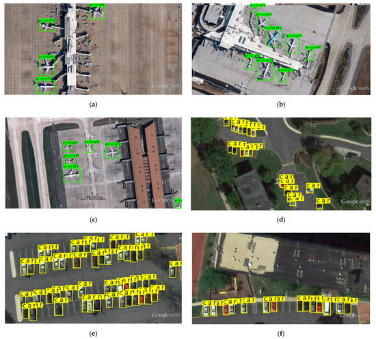
Figure 15. The detection results with the UCS-AOD dataset.

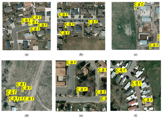
Figure 16. The detection results with the VIDEA dataset.

The detection results on these samples demonstrate the excellent performance of our approach when facing remote sensing targets under with complex backgrounds, in different light conditions or with very small sizes.

4.4.3. Ablation Experiment

The advanced performance of FE-YOLO was exhibited in Section 4.4.1 and Section 4.4.2. In order to analyze the effectiveness of each module for the detection performance of the detector, different compound modes were set in the experiment for comparison. Due to the diversity of target varieties, the RSOD dataset was chosen in an ablation experiment.

In order to verify the effectiveness of our proposed ‘DPFE’ modules in the feature extraction network in Section 3.2, the comparative experimental data are presented in Table 12.

Table 12. The influence of DPFE modules on the RSOD dataset.

	DPFE 1	DPFE 2	AP (%)					FPS
			Aircraft	Oil Tank	Overpass	Playground	mAP (IOU = 0.5)
1			75.52	78.26	79.28	83.45	79.59	69.5
2	√		82.25	83.47	86.23	88.72	84.55	68.4
3		√	83.25	84.49	85.72	87.64	84.80	67.8
4	√	√	86.69	87.57	88.21	92.85	88.83	65.4

In the same way, to verify the effectiveness of our proposed ‘Res2 blocks’ in the feature extraction network in Section 4.4, the comparative data are shown in Table 13.

Table 13. The influence of ‘Res2 blocks’ on RSOD.

	RES2 8	RES2 4	AP (%)					FPS
			Aircraft	Oil Tank	Overpass	Playground	mAP (IOU = 0.5)
1			77.42	79.59	80.43	85.25	80.67	61.3
2	√		83.45	84.57	86.24	89.52	85.95	64.7
3		√	84.15	85.25	86.32	88.68	86.10	63.5
4	√	√	86.69	87.57	88.21	92.85	88.83	65.4

Finally, to verify the effectiveness of our ‘IRFE’ modules in the detection layers in Section 4.3, the comparative date are shown in Table 14.

Table 14. The influence of ‘IRFE’ modules on RSOD dataset.

mAP	FPS	IRFE 1	IRFE 2	IRFE 3
86.24	62.7
87.32	64.5			√
88.43	64.8		√	√
88.83	65.4	√	√	√

The experimental comparison results of ablation experiments in Table 12, Table 13 and Table 14 testify the effectiveness of each modules we proposed.

The above discussion in Section 3.2, and the experiment on ImageNet-1k dataset in [50], proved the superior performance of the Dual Path Network (DPN). Our proposed DPFE modules borrow the ideal of DPN, and the results of the ablation experiments are shown in Table 12. In Table 12, it can be seen that with DPFE modules added in the feature extraction network, the mAP improved from 79.59 to 88.83%. The detection speed did not decline. In addition, when facing small targets like aircraft, the promotion of precision improved even more distinctly. In Table 13, our proposed Res2 blocks improved the performance of remote sensing target detection. The mAP improved from 80.67 to 88.83%.

In Table 14, it can be seen that when the number of IRFE modules increases, the mAP of our model upgrades constantly. Moreover, IRFE modules can improve the detection speed slightly.

The three ablation experiments above-mentioned testify the effectiveness of our improved modules. With DPFE modules and Res2 blocks modules in the feature extraction network, and IRFE modules in the detection layers, the precision of remote sensing target detection improved distinctly. Profiting from the lightweight feature extraction network, the detection speed improved significantly compared with YOLO-V3. Generally speaking, our proposed FE-YOLO is a suitable detector for remote sensing targets.

4.4.4. Extended Experiments

Besides the quantitative experiments aforementioned, the performance of our model ought to be reflected intuitively. In order to testify the superiority of FE-YOLO visually, several comparative detection results were exhibited in Figure 17. In Figure 17, 10 groups of samples are chosen for comparison between YOLO-V3 and FE-YOLO.

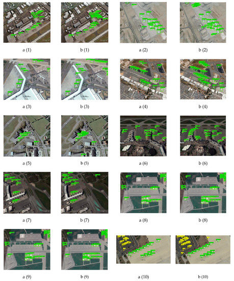
Figure 17. The comparison results of YOLO-V3 and our proposed EF-YOLO: a (1)–a (10) are the detection results of YOLO-V3; b (1)–b (10) are the corresponding detection results of FE-YOLO.

In Figure 17, a total of 20 comparative results of 10 groups are exhibited. The samples we chose contain a large number of small targets, and most of them are densely distributed. In Figure 17, a (1)–a (10) are the detection results of YOLO-V3, while b (1)–b (10) are the detection results of FE-YOLO. The comparative results show that there are several remote sensing targets missing that are detected by YOLO-V3. By contrast, every target in the figures we chose were detected by FE-YOLO.

The employment of the light weighted feature extraction network we proposed greatly reduced redundancy and improved the detection efficiency of the network. Experimental results in Table 12, Table 13 and Table 14 show the effectiveness of the feature enhancement modules and new residual blocks we proposed in Section 3.2, Section 3.3 and Section 3.4. The extended experiments attest intuitively that FE –YOLO is superior to YOLO-V3 in detecting small remote sensing targets.

4.4.5. Antinoise Performance Experiment

In practical applications, remote sensing images are often polluted by noise. So, the performance of antinoise is also important for the detector. In order to assess the antinoise performance of our FE-YOLO, white Gaussian noise of different intensities was added to the test set to compare the influence of noise on accuracy. The experimental results on the RSOD dataset are shown in Table 15.

Table 15. The accuracy under white Gaussian noise of different intensities.

Noise Intensity (dB)	mAP (%)
	SSD	Faster RCNN	YOLO-V3	FE-YOLO
None	72.97	87.76	77.10	88.83
10	68.75	86.22	72.94	87.36
20	61.52	79.62	68.61	83.24
30	52.95	65.42	61.84	77.63

The experimental results in Table 15 show the benign performance of antinoise for our approach. Compared with the performance of the state-of-art detectors, in which the accuracy decreases sharply with increased noise, the accuracy of our FE-YOLO still maintained a high level. From the above experiments, we can see our improved network not only has the better detection accuracy on remote sensing targets, but also has good antinoise performance.

5. Conclusions

For target detection algorithms, detection accuracy and detection speed ought to be taken into account at the same time. In this paper, a new detection model based on YOLO-V3 was proposed. Different from conventional targets, remote sensing targets are usually of small size and under complex backgrounds. Due to the characteristics of remote sensing targets, and giving consideration to detection speed, a series of improvements were taken. First, in order to solve the problem of redundancy in the feature extraction network of YOLO-V3, a new lightweight backbone network was proposed. Second, the lightweight network made it weak for feature extraction. So, two kinds of feature extraction modules we proposed (i.e., DPFE and IRFE) were added to the feature extraction network and detection layers, respectively. Thirdly, two ‘Res2 blocks’ were adopted instead of the original residual blocks in the feature extraction network to increase the range of receptive fields. The experimental results shown in Table 8, Table 9 and Table 10 indicate the excellent performance of our proposed FE-YOLO. In terms of detection speed, the FPS of FE-YOLO was close to that of YOLO-V3. The ablation experimental results in Table 11, Table 12 and Table 13 confirm the effectiveness of each module we proposed. In Section 4.4.2 and Section 4.4.4, Figure 14, Figure 15, Figure 16 and Figure 17 demonstrates the superiority of FE-YOLO visually compared with YOLO-V3. In the detection results of YOLO-V3, there are several targets missing detection. By contrast, FE-YOLO detected almost every remote sensing target labelled. Furthermore, the detection speed was faster than YOLO-V3. Generally speaking, our approach (FE-YOLO) is a suitable detector for remote sensing target detection. In future work, an attentional mechanism will be a key research direction.

References

- Song, X.R.; Gao, S.; Chen, C.B. A multispectral feature fusion network for robust pedestrian detection. Alex. Eng. J. 2021, 60, 73–85. [Google Scholar] [CrossRef]
- Ma, J.; Wan, H.L.; Wang, J.X.; Xia, H.; Bai, C.J. An improved one-stage pedestrian detection method based on multi-scale attention feature extraction. J. Real-Time Image Process. 2021. [Google Scholar] [CrossRef]
- Chen, X.; Zhang, Y.; Lin, L.; Wang, J.X.; Ni, J.Q. Efficient Anti-Glare Ceramic Decals Defect Detection by Incorporating Homomorphic Filtering. Comput. Syst. Sci. Eng. 2021, 36, 551–564. [Google Scholar] [CrossRef]
- Xie, L.F.; Xiang, X.; Xu, H.N.; Wang, L.; Lin, L.J.; Yin, G.F. FFCNN: A Deep Neural Network for Surface Defect Detection of Magnetic Tile. IEEE Trans. Ind. Electron. 2021, 68, 3506–3516. [Google Scholar] [CrossRef]
- Ni, X.C.; Dong, G.Y.; Li, L.G.; Yang, Q.F.; Wu, Z.J. Kinetic study of electron transport behaviors used for ion sensing technology in air/ EGR diluted methane flames. Fuel 2021, 288. [Google Scholar] [CrossRef]
- Alsaadi, H.I.H.; Almuttari, R.M.; Ucan, O.N.; Bayat, O. An adapting soft computing model for intrusion detection system. Comput. Intell. 2021. [Google Scholar] [CrossRef]
- Lee, J.; Moon, S.; Nam, D.W.; Lee, J.; Oh, A.R.; Yoo, W. A Study on the Identification of Warship Type/Class by Measuring Similarity with Virtual Warship. In Proceedings of the 2020 International Conference on Information and Communication Technology Convergence (ICTC), Jeju, Korea, 21–23 October 2020; pp. 540–542. [Google Scholar] [CrossRef]
- Cho, S.; Shin, W.; Kim, N.; Jeong, J.; In, H.P. Priority Determination to Apply Artificial Intelligence Technology in Military Intelligence Areas. Electronics 2020, 9, 2187. [Google Scholar] [CrossRef]
- Fukuda, G.; Hatta, D.; Guo, X.; Kubo, N. Performance Evaluation of IMU and DVL Integration in Marine Navigation. Sensors 2021, 21, 1056. [Google Scholar] [CrossRef]
- Ajayakumar, J.; Curtis, A.J.; Rouzier, V.; Pape, J.W.; Bempah, S.; Alam, M.T.; Alam, M.M.; Rashid, M.H.; Ali, A.; Morris, J.G. Exploring convolutional neural networks and spatial video for on-the-ground mapping in informal settlements. Int. J. Health Geogr. 2021, 20, 5. [Google Scholar] [CrossRef]
- Muller, D.; Kramer, F. MIScnn: A framework for medical image segmentation with convolutional neural networks and deep learning. BMC Med. Imaging 2021, 21, 12880. [Google Scholar] [CrossRef]
- Gao, K.L.; Liu, B.; Yu, X.C.; Zhang, P.Q.; Tan, X.; Sun, Y.F. Small sample classification of hyperspectral image using model-agnostic meta-learning algorithm and convolutional neural network. Int. J. Remote Sens. 2021, 42, 3090–3122. [Google Scholar] [CrossRef]
- Girshick, R.; Donahue, J.; Darrell, T.; Malik, J. Rich feature hierarchies for accurate object detection and semantic segmentation. In Proceedings of the 2014 IEEE Conference on Computer Vision and Pattern Recognition, Columbus, OH, USA, 23–28 June 2014; pp. 580–587. [Google Scholar] [CrossRef]
- Girshick, R. Fast R-CNN. In Proceedings of the 2015 IEEE International Conference on Computer Vision, (ICCV), Santiago, Chile, 7–13 December 2015; pp. 1440–1448. [Google Scholar] [CrossRef]
- Ren, S.Q.; He, K.M.; Girshick, R.; Sun, J. Faster R-CNN: Towards Real-Time Object Detection with Region Proposal Networks. IEEE Trans. Pattern Anal. Mach. Intell. 2016, 39, 1137–1149. [Google Scholar] [CrossRef]
- He, K.M.; Gkioxari, G.; Dollar, P.; Girshick, R. Mask R-CNN. In Proceedings of the 2017 IEEE International Conference on Computer Vision, Venice, Italy, 22–29 October 2017; pp. 2980–2988. [Google Scholar] [CrossRef]
- He, K.M.; Zhang, X.Y.; Ren, S.Q.; Sun, J. Spatial Pyramid Pooling in Deep Convolutional Networks for Visual Recognition. IEEE Trans. Pattern Anal. Mach. Intell. 2015, 37, 1904–1916. [Google Scholar] [CrossRef]
- Wang, X.L.; Wang, S.; Cao, J.Q.; Wang, Y.S. Data-Driven Based Tiny-YOLOv3 Method for Front Vehicle Detection Inducing SPP-Net. IEEE Access 2020, 8, 110227–110236. [Google Scholar] [CrossRef]
- Li, L.L.; Yang, Z.Y.; Jiao, L.C.; Liu, F.; Liu, X. High-Resolution SAR Change Detection Based on ROI and SPP Net. IEEE Access 2019, 7, 177009–177022. [Google Scholar] [CrossRef]
- Lin, T.Y.; Dollar, P.; Girshick, R.; He, K.M.; Hariharan, B.; Belongie, S. Feature Pyramid Networks for Object Detection. In Proceedings of the 30th IEEE Conference on Computer Vision and Pattern Recognition, Honolulu, HI, USA, 21–26 July 2017; pp. 936–944. [Google Scholar] [CrossRef]
- Kim, S.W.; Kook, H.K.; Sun, J.Y.; Kang, M.C.; Ko, S.J. Parallel Feature Pyramid Network for Object Detection. In Computer Vision—ECCV 2018, Proceedings of the 15th European Conference on Computer Vision, Munich, Germany, 8–14 September 2018; Ferrari, V., Hebert, M., Sminchisescu, C., Weiss, Y., Eds.; Springer: Berlin/Heidelberg, Germany, 2018; Volume 11209, pp. 239–256. [Google Scholar]
- Dai, J.F.; Li, Y.; He, K.M.; Sun, J. R-FCN: Object Detection via Region-based Fully Convolutional Networks. In Advances in Neural Information Processing Systems 29, Procedings of the 30th Annual Conference on Neural Information Processing Systems, Barcelona, Spain, 5–10 December 2016; Lee, D.D., Sugiyama, M., Luxburg, U.V., Guyon, I., Garnett, R., Eds.; Curran Associates, Inc.: New York, NY, USA, 2016; Volume 29. [Google Scholar]
- Singh, B.; Davis, L.S. An Analysis of Scale Invariance in Object Detection—SNIP. In Proceedings of the 2018 IEEE/CVF Conference on Computer Vision and Pattern Recognition, Salt Lake City, UT, USA, 18–23 June 2018; pp. 3578–3587. [Google Scholar] [CrossRef]
- Singh, B.; Najibi, M.; Davis, L.S. SNIPER: Efficient Multi-Scale Training. In Advances in Neural Information Processing Systems 31, Proceedings of the Annual Conference on Neural Information Processing Systems, Montréal, Canada, 3–8 December 2018; Bengio, S., Wallach, H., Larochelle, H., Grauman, K., Cesa Bianchi, N., Garnett, R., Eds.; Curran Associates, Inc.: New York, NY, USA, 2019; Volume 31. [Google Scholar]
- Redmon, J.; Divvala, S.; Girshick, R.; Farhadi, A. You Only Look Once: Unified, Real-Time Object Detection. In Proceedings of the 2016 IEEE Conference on Computer Vision and Pattern Recognition (CVPR), Las Vegas, NV, USA, 27–30 June 2016. [Google Scholar]
- Redmon, J.; Farhadi, A. YOLO9000: Better, Faster, Stronger. In Proceedings of the IEEE Conference on Computer Vision and Pattern Recognition (CVPR), Honolulu, HI, USA, 21–26 July 2017; pp. 6517–6525. [Google Scholar]
- Redmon, J.; Farhadi, A.J. YOLOv3: An Incremental Improvement. arXiv 2018, arXiv:1804.02767. [Google Scholar]
- Adarsh, P.; Rathi, P.; Kumar, M. YOLO v3-Tiny: Object Detection and Recognition using one stage improved model. In Proceedings of the 2020 6th International Conference on Advanced Computing and Communication Systems, Coimbatore, India, 6–7 March 2020; pp. 687–694. [Google Scholar]
- Bochkovskiy, A.; Wang, C.Y.; Liao, H.Y.M. YOLOv4: Optimal Speed and Accuracy of Object Detection. arXiv 2020, arXiv:2004.10934. [Google Scholar]
- Liu, W.; Anguelov, D.; Erhan, D.; Szegedy, C.; Reed, S.; Fu, C.Y.; Berg, A.C. SSD: Single Shot MultiBox Detector. In Computer Vision—Eccv 2016, Proceedings of the European Conference on Computer Vision, Amsterdam, The Netherlands, 8–16 October 2016; Leibe, B., Matas, J., Sebe, N., Welling, M., Eds.; Springer: Cham, Switzerland, 2016; Volume 9905, pp. 21–37. [Google Scholar]
- Fu, C.Y.; Liu, W.; Ranga, A.; Tyagi, A.; Berg, A.C. DSSD: Deconvolutional Single Shot Detector. arXiv 2017, arXiv:1701.06659. [Google Scholar]
- Ma, W.; Wang, X.; Yu, J. A Lightweight Feature Fusion Single Shot Multibox Detector for Garbage Detection. IEEE Access 2020, 8, 188577–188586. [Google Scholar] [CrossRef]
- Wang, T.; Anwer, R.M.; Cholakkal, H.; Khan, F.S.; Pang, Y.; Shao, L. Learning Rich Features at High-Speed for Single-Shot Object Detection. In Proceedings of the 2019 IEEE/CVF International Conference on Computer Vision, Seoul, Korea, 27 October–2 November 2019; pp. 1971–1980. [Google Scholar] [CrossRef]
- Shone, R.; Glazebrook, K.; Zografos, K.G. Applications of stochastic modeling in air traffic management: Methods, challenges and opportunities for solving air traffic problems under uncertainty. Eur. J. Oper. Res. 2021, 292, 1–26. [Google Scholar] [CrossRef]
- Xu, Z.; Sun, Y.; Liu, M. iCurb: Imitation Learning-Based Detection of Road Curbs Using Aerial Images for Autonomous Driving. IEEE Robot. Autom. Lett. 2021, 6, 1097–1104. [Google Scholar] [CrossRef]
- Ji, X.; Yan, Q.; Huang, D.; Wu, B.; Xu, X.; Zhang, A.; Liao, G.; Zhou, J.; Wu, M. Filtered selective search and evenly distributed convolutional neural networks for casting defects recognition. J. Mater. Process. Technol. 2021, 292. [Google Scholar] [CrossRef]
- Song, S.-H. H-infinity Approach to Performance Analysis of Missile Control Systems with Proportional Navigation Guidance Laws. J. Electr. Eng. Technol. 2021, 16, 1083–1088. [Google Scholar] [CrossRef]
- Zhang, Q.; Cui, Z.P.; Niu, X.G.; Geng, S.J.; Qiao, Y. Image Segmentation with Pyramid Dilated Convolution Based on ResNet and U-Net. In Neural Information Processing, Proceedings of the International Conference on Neural Information Processing, Guangzhou, China, 14–18 November 2017; Liu, D., Xie, S., Li, Y., Zhao, D., ElAlfy, E.S.M., Eds.; Springer: Cham, Switzerland, 2017; Volume 10635, pp. 364–372. [Google Scholar]
- Oyama, T.; Yamanaka, T. Fully Convolutional DenseNet for Saliency-Map Prediction. In Proceedings of the 4th IAPR Asian Conference on Pattern Recognition, Nanjing, China, 26–29 November 2017; pp. 334–339. [Google Scholar] [CrossRef]
- Long, Y.; Gong, Y.; Xiao, Z.; Liu, Q. Accurate Object Localization in Remote Sensing Images Based on Convolutional Neural Networks. IEEE Trans. Geosci. Remote Sens. 2017, 55, 2486–2498. [Google Scholar] [CrossRef]
- Zhu, H.; Chen, X.; Dai, W.; Fu, K.; Ye, Q.; Jiao, J. ORIENTATION ROBUST OBJECT DETECTION IN AERIAL IMAGES USING DEEP CONVOLUTIONAL NEURAL NETWORK. In Proceedings of the 2015 IEEE International Conference on Image Processing, Quebec City, QC, Canada, 27–30 September 2015; pp. 3735–3739. [Google Scholar]
- Razakarivony, S.; Jurie, F. Vehicle detection in aerial imagery: A small target detection benchmark. J. Vis. Commun. Image Represent. 2016, 34, 187–203. [Google Scholar] [CrossRef]
- Liu, M.J.; Wang, X.H.; Zhou, A.J.; Fu, X.Y.; Ma, Y.W.; Piao, C.H. UAV-YOLO: Small Object Detection on Unmanned Aerial Vehicle Perspective. Sensors 2020, 20, 2238. [Google Scholar] [CrossRef] [PubMed]
- Huang, Z.C.; Wang, J.L.; Fu, X.; Yu, T.; Guo, Y.; Wang, R. DC-SPP-YOLO: Dense connection and spatial pyramid pooling based YOLO for object detection. Inf. Sci. 2020, 522, 241–258. [Google Scholar] [CrossRef]
- Zhang, S.; Mu, X.; Kou, G.; Zhao, J. Object Detection Based on Efficient Multiscale Auto-Inference in Remote Sensing Images. IEEE Geosci. Remote. Sens. Lett. 2020, 1–5. [Google Scholar] [CrossRef]
- Ding, X.; Yang, R. Vehicle and Parking Space Detection Based on Improved YOLO Network Model. J. Phys. Conf. Ser. 2019, 1325, 012084. [Google Scholar] [CrossRef]
- He, W.; Huang, Z.; Wei, Z.; Li, C.; Guo, B. TF-YOLO: An Improved Incremental Network for Real-Time Object Detection. Appl. Sci. 2019, 9, 3225. [Google Scholar] [CrossRef]
- Hu, Y.; Wu, X.; Zheng, G.; Liu, X. Object Detection of UAV for Anti-UAV Based on Improved YOLO v3. In Proceedings of the 2019 Chinese Control Conference (CCC), Guangzhou, China, 27–30 July 2019. [Google Scholar]
- Long, X.; Deng, K.; Wang, G.; Zhang, Y.; Wen, S. PP-YOLO: An Effective and Efficient Implementation of Object Detector. arXiv 2020, arXiv:2007.12099. [Google Scholar]
- Chen, Y.; Li, J.; Xiao, H.; Jin, X.; Yan, S.; Feng, J. Dual Path Networks. arXiv 2017, arXiv:1707.01629. [Google Scholar]
Publisher’s Note: MDPI stays neutral with regard to jurisdictional claims in published maps and institutional affiliations. |
© 2021 by the authors. Licensee MDPI, Basel, Switzerland. This article is an open access article distributed under the terms and conditions of the Creative Commons Attribution (CC BY) license (https://creativecommons.org/licenses/by/4.0/).