Unsupervised Adversarial Domain Adaptation with Error-Correcting Boundaries and Feature Adaption Metric for Remote-Sensing Scene Classification

Abstract

Unsupervised domain adaptation (UDA) based on adversarial learning for remote-sensing scene classification has become a research hotspot because of the need to alleviating the lack of annotated training data. Existing methods train classifiers according to their ability to distinguish features from source or target domains. However, they suffer from the following two limitations: (1) the classifier is trained on source samples and forms a source-domain-specific boundary, which ignores features from the target domain and (2) semantically meaningful features are merely built from the adversary of a generator and a discriminator, which ignore selecting the domain invariant features. These issues limit the distribution matching performance of source and target domains, since each domain has its distinctive characteristic. To resolve these issues, we propose a framework with error-correcting boundaries and feature adaptation metric. Specifically, we design an error-correcting boundaries mechanism to build target-domain-specific classifier boundaries via multi-classifiers and error-correcting discrepancy loss, which significantly distinguish target samples and reduce their distinguished uncertainty. Then, we employ a feature adaptation metric structure to enhance the adaptation of ambiguous features via shallow layers of the backbone convolutional neural network and alignment loss, which automatically learns domain invariant features. The experimental results on four public datasets outperform other UDA methods of remote-sensing scene classification.

1. Introduction

Remote-sensing scene classification, which aims to automatically assign a semantic label to each scene image, has been an active research topic in the field of high-resolution satellite imagery in the past decades [1]. With the rapid development of satellite techniques, an abundance of remote sensing images offers many more capability for scene classification applications, such as geospatial object detection, urban planning, and environment monitoring. In the early stage of development, traditional machine learning methods have been used for scene classification tasks, such as support vector machine and bag of words [2,3]. Recently, deep learning methods have been proven to be effective for extracting image features [4,5,6,7,8], and many studies have demonstrated effective scene classification performance with the help of deep learning from various novel perspectives including self-supervised learning [9], data augmentation [10], feature fusion [11,12,13,14,15], reconstructing networks [16,17,18,19,20,21,22,23], integration of spectral and spatial information [24], balancing global and local features, refining feature maps through encoding method [25], adding a new mechanism [26,27], as well as introducing a new network [28], open set problem [29], and noisy label distillation [30]. However, a lack of annotated data has restricted the development of deep learning methods in scene classification due to the high cost of annotating data. To relieve this problem, fine-tuning [5], data augmentation [31], semi-supervised methods [32,33], and few-shot learning [34] have been applied to improve the utilization efficiency of training samples, however, they are also restricted by label scale and do not achieve unsupervised learning. In fact, we can easily obtain large amounts of unlabeled samples but do not want to deal with the cost for manual annotation. To effectively utilize the abundance of unlabeled data, unsupervised domain adaptation, bridging the gap of domain shift between a source domain (with labels) and a target domain (without labels) has proven to be effective to solve the problem of unlabeled data, and therefore is attracting significant research attention. Through unsupervised domain adaptation, we can extract features from unlabeled data with the help of existing feature knowledge from annotated data.

Unsupervised domain adaptation assumes that both the source and target data are related domains under different space feature distributions, and it intends to align the data distributions of the two domains to achieve knowledge transfer [35]. The discrepancy metric-based method and adversarial-based method are two commonly used methods for unsupervised domain adaptation to achieve feature alignment [18]. The discrepancy metric-based method usually designs a metric to measure the distribution discrepancy of the source and target domain, and then minimizes the metric to align the two domains [36,37]. Pan et al. [38] proposed transfer component analysis (TCA) which attempted to learn some transfer components across domains in a reproducing kernel Hilbert space using maximum mean discrepancy. They skillfully applied knowledge transfer in machine learning and introduced a new life cycle for unsupervised domain adaptation. Long et al. [39] simultaneously reduced the differences in both the marginal and conditional distribution between domains. With the development of deep learning methods, Tzeng et al. [36] applied deep networks for domain adaptation and constructed a basic framework, deep domain confusion (DDC), with maximum mean discrepancy (MMD) [40] for deep metric-based methods. On the basis of the framework of DDC, Long et al. [37] proposed deep adaptation networks (DANs) and considered multiple layer adaptation with multiple kernel variants of MMD [41]. The theory of these methods has been widely used in remote scene classification. Li et al. [42] proposed cross-domain distance metric learning to achieve knowledge transfer for a limited target domain. Zhang et al. [19] proposed a correlation subspace dynamic distribution alignment method with subspace correlation maximization and dynamic statistical distribution alignment to improve domain alignment. Song et al. [43] proposed a subspace alignment based on convolutional neural network (CNN) framework through adding a new subspace alignment layer and fine-tuning the modified CNN model to the aligned feature subspace which helped to relieve the domain distribution discrepancy. However, manually designing a proper metric is difficult, especially for remote sensing images; some complex characteristics increase the difficulty of matching different data domains, such as texture, radiation change, and background. Therefore, many studies have focused on adversarial-based methods and applied the concept of generative adversarial networks (GANs) [44] that set a domain discriminator to discriminate whether the sample is from the source or target domain and set a generator which improves the extracted features to make the discriminator confused and unable to distinguish the sample domain. Then, after training the model, the two domains are adaptively aligned when a balance between the discriminator and generator is established. The idea of adversarial-based methods was first proposed by Ganin et al. [45]. Then, it was widely applied in remote-sensing scene classification. Recently, Pan et al. [31] applied GANs to improve image diversity, and therefore classification performance for more diverse scene structures and essential features. Rahhal et al. [46] used a minmax entropy approach based on optimizing in an adversarial manner the conditional entropy of the target samples with respect to each source classifier. Bejiga et al. [47] introduced a domain adversarial neural network for large-scale land cover classification. Liu et al. [48] proposed an adversarial domain adaptation method boosted by a domain confusion network to adapt the images from different domains to appear as if drawn from the same domain. Lu et al. [18] used multiple complementary source domains to form the categories of the target domain based on an adversarial manner between feature extractor and the cross-domain alignment module.

Although these works have achieved improvements using adversarial networks, the discriminator only distinguishes input data samples into a special domain rather than a class. When the source and target domains are matched, a classifier boundary trained on the source domain is applied directly to the target domain, but it is not specific to the target domain and can lead to some improper discrimination, as shown on the left side of Figure 1. It reduces the performance of satisfactory matching for the two domains, since the data distribution in each domain has individual characteristics. In addition, on the one hand, some target samples that are easily classified into incorrect classes have distinguished uncertainty and can cause confusion for a specific classifier boundary, which also reduces the performance of target-domain-specific boundaries. On the other hand, they extract semantically meaningful features merely based on the adversarial manner between the generator and the discriminator, but they ignore selecting the domain invariant features from each domain. In fact, it is well known that overlap information benefits a cross-domain task. Thus, a key for cross-domain methods is to learn more comprehensive features in two domains. A previous work by [49] has proven that the shallow layers in a convolutional neural network (CNN) contain common features that can be universally used for detecting the objectives, which provide a way to learn the domain invariant features.

In order to resolve the above two issues, we propose an error-correcting boundaries mechanism with feature adaptation metric (ECB-FAM) structure for remote-sensing scene classification, which can train significant target-domain-specific boundaries with the help of error-correcting for the classifier to accurately distinguish the target sample into a special class, and select domain invariant features from the source and target domains, and therefore further improve domain alignment. The proposed ECB-FAM structure has an adversarial manner to balance adversary between the generator and discriminator through an error-correcting boundaries mechanism (ECB) and a feature adaptation metric (FAM) structure. Specifically, the ECB involves multiple classifiers and their discrepancy loss, among which at least one classifier has an error-correcting individuality to rectify the inaccurate discrepancies of classifier mutual predictions for target samples, as shown on the right side of Figure 1. It can calculate an error-correcting discrepancy loss to help the adversary between the generator and discriminator with the target-domain-specific classifier boundaries to improve applicability for predictions of the target domain. The FAM structure is made up of an alignment loss and the shallow layers of the backbone CNN with a fully convolutional network whose kernel size is equal to one. The shallow layers with fully convolutional network are designed to capture domain invariant features to enhance domain matching, with the alignment loss used to measure the differences of ambiguous features between the source and target domains. Finally, when a balance of the adversarial manner is established, it means that the two domains are better aligned based on target-domain-specific boundaries and domain invariant features.

The contributions of our model are as follows:

• To improve the performance of aligning data distribution of source domain and target domain, we propose an adversarial framework with the help of target-domain-specific classifier boundaries and domain invariant features.
• To improve the ability of target-domain-specific classifier boundaries, we design an error-correcting boundaries mechanism to correct errors of misclassification for target samples, which can reduce distinguished uncertainty for difficultly classified target samples.
• To achieve adaptation for ambiguous features, we propose a feature adaptation metric structure to build the domain invariant features and semantically meaningful features simultaneously.
• We conduct comprehensive experiments to demonstrate the effect of the ECB-FAM structure with optional variants for each component. The results show the proposed method can enhance feature extraction and domain matching to improve accuracy of scene classification. In addition, the sub-experiments show the effect of each component.

2. Materials and Methods

As shown in Figure 2, ECB-FAM consists of the following three main components: a feature extractor, an error-correcting boundaries mechanism, and a feature adaptation metric structure. We introduce the training steps of our model in detail in the next subsections.

2.1. Notation and Model Overview

We denote $D_s$ as the source domain and $D_t$ as the target domain. In each data domain, the distribution of data samples is denoted as $d(p)$. $x^s$ and $x^t$ are the samples from $D_s$ and $D_t$, respectively, and y is the data label for $x^s$. If the source domain is similar to the target domain but $d^s(p)\ne d^t(p)$, the transfer learning in this condition is called domain adaptation. Furthermore, if there is no label for the data in the target domain, we call it unsupervised domain adaptation. The purpose of unsupervised domain adaptation is to align $D_s$ and $D_t$, so that the classifier trained on $D_s$ can be used for $D_t$. In summary, the aim of the proposed ECB-FAM structure is to improve the matching degree of $D_s$ and $D_t$, and distinguish target samples into special classes. Additionally, the multiple classifiers and the feature extractor are regarded as the discriminator and generator to implement the adversarial manner, indicated as $C_k$ and $G$, respectively, where k is the index for the multiple classifiers. Generally, the default number of classifiers in the ECB-FAM structure is three. The feature generator is the classical CNNs without the classifier, and we usually use ResNet-50 [8]. All data samples are input into the feature extractor. All the notations are listed in

Table 1. Notations in this work.

Notation	Description
i, k, m	Index
$D_s$	Source domain
$D_t$	Target domain
$d(p)$	Data distribution
$x^s$	Sample of source domain
$x^t$	Sample of target domain
y	Label for source domain sample
$C_k$	Classifier (discriminator)
G	Generator (feature extractor)
T	Number of classes
N,$n_s$, M, $n_t$	Number of samples for source domain or target domain
$\widehat{y}$	Prediction of classifier for y
L	Loss
$L_{C_k}(x^s,y)$	Loss from classifier k for $x^s$
$L_{ad}(x^t)$	Adversarial loss
$L_{sa}^{*}$	Loss of shallow alignment for the source or target domain
p	class probability of classifier for
$d(p_i,p_j)$	Classifier discrepancy
$F_{sa}$	Output of a certain layer
W or H	Width of $F_{sa}$ or height of $F_{sa}$
w or h	Index for width or height of the matrix of $F_{sa}$
$D_{sa}{(F_{sa}(x_i^{*}))}_{wh}$	output of alignment module in each location

.

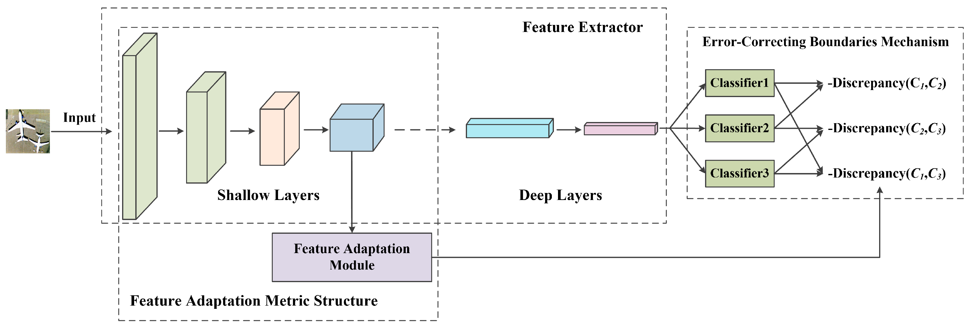
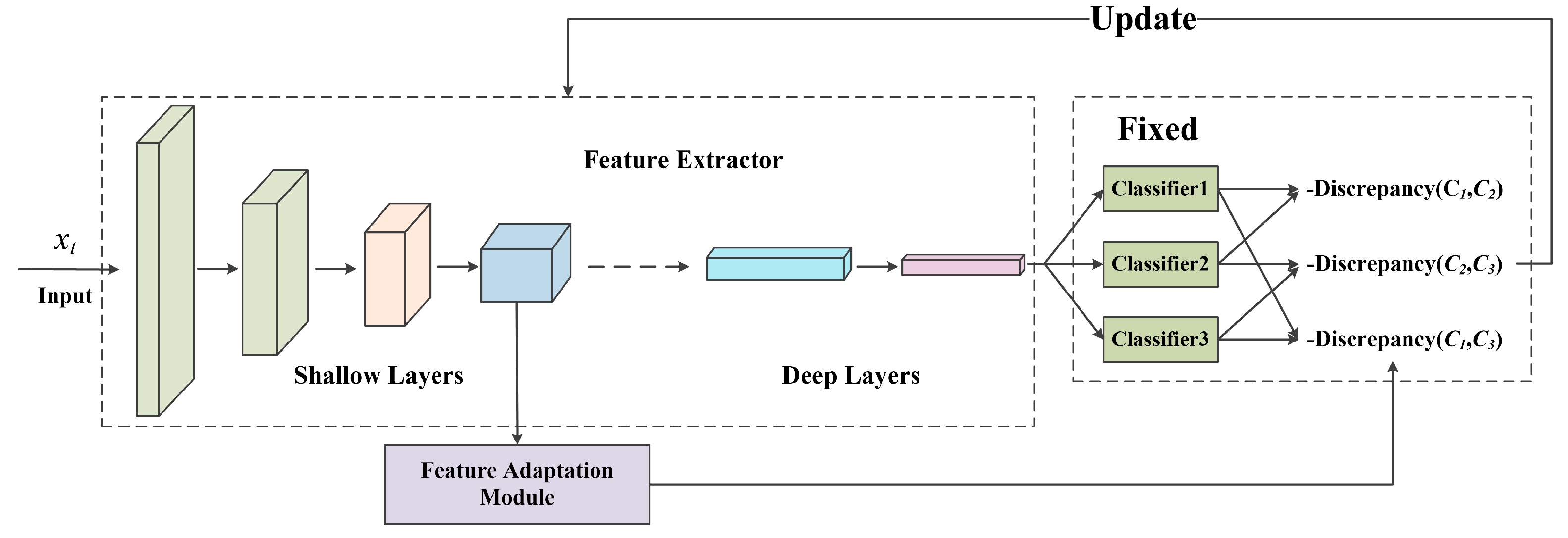
2.2. The Architecture of Error-Correcting Boundaries Mechanism with Feature Adaptation Metric (ECB-FAM)

2.2.1. Adversarial Manner

The principle of the adversarial manner of the ECB-FAM is shown in Figure 3. The adversarial manner of ECB-FAM is also applied between the discriminator and the generator, which is similar to the normal adversarial methods, but the discriminator and generator have their new special components. The discriminator is formed by multiple classifiers of the error-correcting boundaries mechanism, and the generator consists of a backbone CNN (feature extractor) and the feature adaptation metric structure. The adversarial manner in our proposed framework contains two key steps.

First of all, before applying adversarial manner, as shown on the left side of Figure 3, there is only a small region where the target domain is consistent with the source domain, namely the overlap area of the source domain circle and the target domain circle. Most of the target domain is a shadow region which indicates this region needs to be aligned with the source domain. At this moment, the classifiers (two dotted lines) can distinguish the source domain but only a part of the target domain, and the two domains have not been matched.

(1) The discriminator tries its best to search target samples whose distributions are not aligned with the source domain. To this end, we calculate an error-correcting discrepancy among the classifiers of the ECB and maximize the discrepancy to find out more unaligned target samples. The concrete calculation is shown in the next section. As shown on the left side of Figure 3, with maximizing the discrepancy, the classifiers are trained to distinguish more ambiguous target samples, namely the solid lines displaced from the dotted line, which causes the shadow region above the classifiers expanding.

(2) The generator tries its best to improve the extracted feature quality to make the classifiers distinguish the target samples correctly, which matches the distributions between the unaligned target samples and the source domain. To this end, we minimize the error-correcting discrepancy and optimize the feature extractor. Furthermore, another designed alignment loss is also added in the optimization of the feature extractor. The concrete calculation is shown in the next section. As shown in the middle part of Figure 3, with minimizing the error-correcting discrepancy and alignment loss, on the one hand, more target samples are matched with the source domain, namely the overlap of the two domain circles expanding; on the other hand, the classifiers can distinguish more target samples correctly, namely the region below the classifiers expanding. As we can see, at this moment, unaligned region of target domain is reduced.

When iterations of the two above steps are implemented, the final alignment of the source domain and the target domain will be achieved, as on the right side of Figure 3. Note that the adversarial manner used for matching the source and target domains is on the premise of correct classification of classifiers for the source domain. The details of the ECB, the FAM structure, and the calculations of the proposed framework are shown in the next section.

2.2.2. Error-Correcting Boundaries Mechanism

In detail, the ECB consists of the discrepancy loss and multiple classifiers (default is three classifiers) in which one of these classifiers is an error-correcting classifier and the others are discrepancy classifiers.

The core of the ECB is the calculation of the error-correcting discrepancy. As we know, different classifiers with the same extracted features for a target sample may assign different predictions, which provide the basis for calculating the error-correcting discrepancy. Each classifier applies Softmax to calculate the class probabilities through a T-dimensional vector of the classifier (T is equal to the number of classes of target domain), and it is given as follows:

$$p_k=\mathrm{softmax}(C_k(G(x^t)))$$

(1)

Furthermore, we set a probability distance to measure the discrepancy between two classifiers, as shown in the following:

$$d(p_i,p_j)=\frac{1}{M}{\displaystyle \sum _{m=1}^M|p_{im}-p_{jm}|}$$

(2)

Equation (2) is used to find out more target samples which are not matched with the source domain. When the discrepancy loss is 0, it means the target samples are classified correctly by both classifiers.

However, when we use two classifiers to calculate discrepancy, some prediction errors will reduce the accuracy of the discrepancy. When $d(p_i,p_j)=0$ for a target sample $x_m^t$, it originally means the classifiers assign the same prediction and they consider $x_m^t$ has been aligned with the source domain. However, if the classifiers both assign $x_m^t$ the same incorrect prediction, the discrepancy will provide distortion although $d(p_i,p_j)=0$.

To indicate this error, we show an example. Obviously, there are four conditions for a pair of classifiers for the prediction of the same target sample $x_m^t$, as Figure 4a–d show. Only the different predictions (a and c) or the same correct prediction (d) for $x_m^t$ can achieve the positive discrepancy calculation. However, the same incorrect prediction for $x_m^t$ (b) is inconsistent with the ground-truth, while it is considered as a correct prediction since $d(p_1,p_2)=0$. Therefore, we set another error-correcting classifier to redress the distortion. When we use three classifiers, the probability of all three classifiers giving the same incorrect prediction can be reduced as compared with that of two classifiers, which improves the accuracy of the classifier discrepancy for searching more unaligned target samples.

Thus, the new error-correcting discrepancy is calculated as Equation (3) as follows:

$$L_{ad}(x_t)=d(p_1,p_2)+d(p_1,p_3)+d(p_2,p_3)$$

(3)

The error-correcting discrepancy is also a part of adversarial loss to optimize the framework.

2.2.3. Feature Adaptation Metric Structure

In detail, FAM consists of the shallow layers of the feature extractor with feature adaptation module and an alignment loss, and it is a part of the generator to confuse the discriminator. On the one hand, the feature extraction ability of the generator is improved by minimizing the error-correcting discrepancy; on the other hand, we can improve the feature extractor using the FAM structure.

The features in the shallow layers of CNNs are often the common local structures for the objectives [50], which can be seen as ambiguous features since they are similar to each other. Previous studies have usually aimed to align semantic information among high-level features in CNNs, but these features contain a lot of special semantics for particular objects and their alignments usually cause alignment attenuation. On the contrary, common features do not contain obvious semantics for the objects in a scene as compared with the high-level features, therefore, we are forced to align them so the source and target domains do not cause negative influence but benefit the adaptation. Therefore, we set a feature adaptation metric for alignment of the shallow layers in the feature extractor.

The structure of the alignment module contains a fully convolutional network, $F_c$, whose kernel size is equal to one, which helps to nonlinear the extracted features. The input of the feature adaptation module is the feature map from the shallow layers, $F_{sa}$, for the source domain samples, $x^s$, and the target domain samples, $x^t$, respectively. Note that parameter sharing is used in the module. Through $F_c$, the outputs from the two domains are aligned empirically with a least-squares loss [50,51] which is used to measure the differences between the feature maps of the shallow layer from the source and target domain as follows:

$$L_{sa}^s=\frac{1}{n_{s}WH}{\displaystyle \sum _{i=1}^{n_s}{\displaystyle \sum _{w=1}^W{\displaystyle \sum _{h=1}^H{D}_{sa}{(F_{sa}(x_i^s))}_{wh}^2}}}$$

(4)

$$L_{sa}^t=\frac{1}{n_{t}WH}{\displaystyle \sum _{i=1}^{n_t}{\displaystyle \sum _{w=1}^W{\displaystyle \sum _{h=1}^H{(1-D_{sa}{(F_{sa}(x_i^t))}_{wh})}^2}}}$$

(5)

where $L_{sa}^{*}$ denotes the loss of alignment, and W and H are the width and height of the input; $D_{sa}{(F_{sa}(x_i^{*}))}_{wh}$ denotes the output of the feature adaptation module in each location; $n_s$ and $n_t$ are the sample number for the source and target domain, respectively; $x^s$ and $x^t$ are the sample of the source and target domains, respectively; and $i$, $w$, and $h$ are the indexes for $n_{*}$, W, and H. As we can see, in the process of alignment, $F_{sa}$ is the feature map from the shallow layers and it is obtained by inputting $x^s$ and $x^t$ into the shallow layers of the feature extractor $D_{sa}$, that is, the module is designed to align each receptive field of features with another domain.

2.3. Training Step

In this section, according to the principle of ECB-FAM, we detail a three-step method which includes training the model on the source domain, maximizing cross-classifier discrepancy for the target domain, and optimizing the feature extractor. The first step is to train good classifiers that can distinguish source domain correctly, so that the classifiers can have the ability to identify the target domain samples that are different from the source domain. The second step is to try the best to find out the target domain samples that are different from the source domain, which is one hand for the adversarial manner. The third step is to improve the feature extractor, so that it can confuse the classifiers and align the source domain and the target domain, and train a task-specific classifier boundary simultaneously, which is another hand for the adversarial manner. Note that the second step will optimize the classifiers based on fixing the feature extractor. On the contrary, the third step will optimize the feature extractor based on fixing the classifiers. Finally, the alternate iteration of the second and third steps is implemented until a balance of adversarial manner is established. In detail the three-step method is as follows:

Step 1 Training the model on the source domain.

As Figure 5 shows, in this step, we feed the model source domain samples with labels, which is similar to other adversarial domain adaptation frameworks to train the model on source data. We set three classifiers under the same construction but different initial parameters which can guarantee the classifiers have some minor decision for the target domain in the next step. This step can make the classifiers distinguish the source domain correctly when achieving model convergence. In this phase, cross-entropy is used to measure the discrepancy between the prediction and the ground-truth label as follow:

$$L_{C_k}(x^s,y)=-\frac{1}{N}{\displaystyle \sum _{i=1}^N(y_{ki}\log ({\widehat{y}}_{ki})+(1-y_{ki})\log (1-{\widehat{y}}_{ki}))}$$

(6)

where $y$ is the label and ${\widehat{y}}_{ki}$ is the prediction of the corresponding $y$ for the kth classifier. Note that we need to train all three classifiers and the generator, and loss function should be separately used for every classifier. The generator and discriminator are both optimized as Equation (7) as follows:

$$\underset{C_1,C_2,C_3,G}{\min }{L}_{C_k}(x^s,y)$$

(7)

Step 2 Maximizing cross-classifier discrepancy for the target domain.

As Figure 6 shows, in this phase, only the discriminator is updated with the fixed generator. All three classifiers are attached behind the feature extractor to predict the label of the current target sample. The discrepancy is the sum of the whole distance functions among multiple classifiers, as shown in Equation (3).

In this step, we optimize the classifiers with the error-correcting discrepancy loss and classification loss, as shown in the following Equation (8) (note that minimizing $-L_{ad}(x^t)$ is equal to maximizing the error-correcting discrepancy):

$$\underset{C_1,C_2,C_3}{\min }{L}_{C_k}(x^s,y)-L_{ad}(x^t)$$

(8)

Step 3 Optimizing the feature extractor.

As Figure 7 shows, in this step, we only update the generator with the fixed parameters of the three classifiers. The loss of improving the feature extractor contains two parts. One is the alignment loss in the shallow layers. The other is to minimize the error-correcting discrepancy loss to make the discriminator classify the target samples better. Therefore, integrated loss is shown by Equation (9) as:

$$\underset{G}{\min }{L}_{sa}(F_{sa},D_{sa})+L_{ad}(x^t)$$

(9)

Then, all steps are repeated until the best model parameters are obtained. The entire algorithm of the proposed ECA-FAM structure is listed in Algorithm 1.

Algorithm 1. Algorithm for training the ECA-FAM structure.

Training Steps

Input: $x^s$, y, and $x^t$, Output: accuracy of classifying $x^t$

input $x^s$, y, $x^t$ foriin epoch:   calculate $L_{C_k}(x^s,y)=-\frac{1}{N}{\displaystyle \sum _{i=1}^N(y_{ki}\log ({\widehat{y}}_{ki})+(1-y_{ki})\log (1-{\widehat{y}}_{ki}))}$   optimize G and $C_k$ with $\underset{C_1,C_2,C_3,G}{\min }{L}_{C_k}(x^s,y)$   for k in number of classifiers:     calculate $p_k=softmax(C_k(G(x^t)))$ and $d(p_i,p_j)=\frac{1}{M}{\displaystyle \sum _{m=1}^M|p_{im}-p_{jm}|}$   calculate $L_{ad}(x_t)=d(p_1,p_2)+d(p_1,p_3)+d(p_2,p_3)$   calculate $L_{C_k}(x^s,y)-L_{ad}(x^t)$   optimize $C_k$ with $\underset{C_1,C_2,C_3}{\min }{L}_{C_k}(x^s,y)-L_{ad}(x^t)$   for w, h in W, H:     calculate $L_{sa}^s=\frac{1}{n_{s}WH}{\displaystyle \sum _{i=1}^{n_s}{\displaystyle \sum _{w=1}^W{\displaystyle \sum _{h=1}^H{D}_{sa}{(F_{sa}(x_i^s))}_{wh}^2}}}$     calculate $L_{sa}^t=\frac{1}{n_{t}WH}{\displaystyle \sum _{i=1}^{n_t}{\displaystyle \sum _{w=1}^W{\displaystyle \sum _{h=1}^H{(1-D_{sa}{(F_{sa}(x_i^t))}_{wh})}^2}}}$   calculate $L_{sa}(F_{sa},D_{sa})+L_{ad}(x^t)$   optimize G with $\underset{G}{\min }{L}_{sa}(F_{sa},D_{sa})+L_{ad}(x^t)$ end for return accuracy of classifying $x^t$

3. Results

3.1. Datasets and Experimental Setting

The experimental datasets used are UC Merced (UCM) [52], NWPU-RESISC45 (NWPU) [53], RSI-CB256 (RSI) [54], and WHU-RS19 (WHU) [55]. They are manually extracted from aerial orthoimages covering various urban areas or Google Earth. UCM contains 21 classes; each class consists of 100 images with the size 256 $\times$ 256 pixels and RGB bands. NWPU contains 45 classes; each class is composed of 700 images with the size 256 $\times$ 256 pixels and RGB bands. RSI contains 35 classes; each class consists of about 690 images with the size 256 $\times$ 256 pixels and RGB bands. WHU contains 19 classes; each class consists of 50 images with the size 600 $\times$ 600. We conduct experiments on these datasets because they have more scenes than other public datasets.

Because there is no specialized dataset for transfer learning research in remote-sensing scene classification, we combine the four different public datasets of scene classification and build some new sub-datasets with the common classes to test knowledge transfer. Specifically, we randomly select two datasets as the source domain and target domain, respectively, and the corresponding common categories of the two datasets are used for training and test data. Due to containing far fewer samples, WHU is only used as a target domain. As a result, the detailed common classes are listed in

Table 2. Common categories of datasets.

Datasets	Common Categories
U and N	Airplane, baseball diamond, beach, chaparral, dense residential, forest, freeway, golf course, harbor, intersection, medium residential, mobile home park, overpass, parking lot, river, runway, sparse residential, storage tank, and tennis court
U and R	Airplane, beach, forest, harbor, intersection, parking lot, residential, river, and storage tank
U and W	Beach, dense residential, forest, parking lot, and river
N and R	Airplane, beach, bridge, desert, forest, harbor, intersection, medium residential, mountain, parking lot, river, and storage tank
N and W	Airport, beach, bridge, commercial area, dense residential, desert, forest, harbor, industrial area, meadow, mountain, parking lot, railway station, and river
R and W	Beach, bridge, desert, forest, harbor, mountain, parking lot, residential, and river

, and we form nine pairs of source and target domain, and they are shown in

Table 3. Main hyperparameters of competitors in this work.

Methods	Settings
TCA	Following the settings of JDA with classes which are set to 0
JDA	Subspace bases is set to 100 Regularization parameter is set to 1.0 Gaussian kernel with a bandwidth in a range of [0.001,1]
DAN	Stochastic gradient descent (SGD) with 0.9 momentum Learning rate with annealing strategy: base rate between 10−5 and 10−2 with a multiplicative step-size 101/2
CORAL	Base learning rate is set to 10−3, weight decay to 5 × 10−4, and momentum to 0.9
CycleGAN	Learning rate of 0.0005 with 0.8 and 0.999 momentums for Adam
GTA	Base learning rate of 0.0005 and momentum 0.8 for Adam Cost coeffificient α and β are both set as 0.01.
DANN ADA-BDC	Learning rate 0.001 with 0.9, batch size for Adam Learning rate of 0.0005 with 0.8 and 0.999 momentums for Adam

. For convenience, we abbreviate the four datasets to U (UCM), N (NWPU), R (RSI), and W (WHU). The detailed samples of common categories for the two datasets are listed in Figure 8, Figure 9, Figure 10, Figure 11, Figure 12 and Figure 13. Furthermore, the dataset as the target domain is divided into a training set and a test set at the ratio of 80% and 20%. The results are the average for five times. We used Adam [56] to optimize our model and the learning rate is set to 0.001 with 0.5 decay per 10 epochs. We set the batchsize to 128. ResNet-50 [8] is used as the backbone CNN for the generator. We conduct the experiment in Pytorch and on GPU NVIDIA Tesla T4.

3.2. Experimental Results

We compare the ECB-FAM with some recent state-of-the-art methods for unsupervised domain adaptation, including TCA [38], joint distribution adaptation (JDA) [39], DAN [37], CORAL [57], cycle consistent generative adversarial network (CycleGAN) [52], generate to adapt (GTA) [58], deep adversarial neural network (DANN) [45], and unsupervised adversarial domain adaptation method boosted by a domain confusion network (ADA-BDC) [49]. The hyperparameters of these comparisons are set according to their original references to get the best results, as shown in Table 3. We test these methods on the combinations of the four datasets, and the results are presented in

Table 4. Detailed results of the proposed framework comparing with the baseline methods. Accuracy (% as the unit) is used as the metric.

Methods	U→N	N→U	U→R	R→U	U→W	N→R	R→N	N→W	R→W
TCA	35.68	67.41	71.52	62.27	42.09	44.55	45.64	80.38	54.69
JDA	41.57	63.74	76.07	63.36	67.33	45.67	48.05	81.24	61.48
DAN	48.85	62.34	81.91	74.35	71.57	55.26	43.72	77.68	70.03
CORAL	36.73	57.85	78.61	66.04	82.37	55.17	45.38	78.62	70.33
CycleGAN	55.83	61.72	87.53	77.71	73.06	62.51	47.69	67.35	74.08
GTA	57.42	73.63	86.13	81.23	89.51	74.65	55.77	84.03	74.98
DANN	52.33	66.58	84.93	76.57	88.14	72.28	52.91	79.36	71.18
ADA-BDC	56.01	74.44	88.47	82.04	91.15	79.58	59.66	82.49	76.57
ECB-FAM	59.10	79.37	90.81	83.74	91.31	81.54	62.64	86.38	79.77

. Compared with other recent unsupervised domain adaptation methods, we can see that the ECB-FAM structure outperforms other baselines with a relatively large margin. Specifically, as compared with classical transfer learning without deep learning (TCA and JDA), other methods based on deep learning are almost beyond them, which indicates deep learning methods offer effective improvements in unsupervised domain adaptation. Then, the methods through an adversarial manner generally outperform the methods with distance metric based on deep networks (DAN and CORAL), which accords with the present situation that adversarial methods perform better than distance metric methods because manually designing a proper metric is usually difficult. Furthermore, our proposed ECB-FAM structure outperforms other adversarial methods on the whole experimental items, and most of performances exceed about 2%, except the result on U→W, and some performances are better than others with 5% around, which indicate our framework can improve the matching degree of source and target domains by learning a target-specific classification boundary for improving the accuracy of scene classification and finding out the domain invariant features of the two domains. We suppose that the different accuracies on various experimental items are because the image distributions of the datasets are different from each other. It is common that some complex factors can often change the data distribution a lot, such as background ratio, shooting angle, and seasonal variation, even though they do not look very different by the naked eye.

4. Discussion

4.1. Influence of Feature Adaptation Metric Structure

To demonstrate the effect of the FAM structure, we tested the ECB-FAM structure with feature adaptation module by changing the number of convolutional layers participating in the adaptation, including the variant without feature adaptation module (ECB), the variant with one convolutional layer (ECB-FAM-1), the variant with two convolutional layers (ECB-FAM-2), the variant with three convolutional layers (ECB-FAM-3), the variant with four convolutional layers (ECB-FAM-4), and the variant with five convolutional layers (ECB-FAM-5). As Figure 14 shows, the results for ECB-FAM-N are generally better than the ECB for the corresponding experimental items, which show the positive influence of the domain invariant features for domain alignment. We suppose the common structures of the two domains have relevance but also provide ambiguously semantic features before feature adaptation. After achieving feature adaptation, domain invariant features are learned and help to improve domain matching. Especially, ECB-FAM-4 gets the best performance in general, which shows the alignment effect has a positive correlation with the number of layers increasing but much more layers will reduce the adaptation. We suppose that the reduction may be because the deeper layer has many specific features for a certain data domain, and force alignment for it may cause a negative influence. It may need an advanced metric to measure the discrepancy for the specific features. In fact, the features learned in the shallow layers of a neural network are the common objective structures for different data distributions and learning to match the common features of the source and target domain is reasonable.

4.2. Influence of Multiple Classifiers on the Error-Correcting Boundaries Mechanism

To explore the influence on the number of classifiers, we compared the ECB-FAM with three classifiers to its variant with two classifiers and its variant with four classifiers. The principle of variant applies two classifiers or four classifiers to calculate the discrepancy of the target domain which is similar to that of ECB-FAM with three. As Figure 15 shows, we can see that ECB-FAM with three classifiers achieves the best results as compared with others and ECB-FAM with four classifiers is better than ECB-FAM with two classifiers. These results demonstrate that the proposed error-correcting boundaries mechanism has a positive effect to redress the incorrect predictions. The results of the ECB-FAM with three classifiers and the ECB-FAM with four classifiers are similar, and we suppose the reason is because three classifiers reduce the incorrect predictions to a good performance, and more classifiers may achieve a minor improvement but have some impact on each other for predicting target samples due to the parameters, which cause a slight reduction in accuracy. In summary, the results demonstrate that more classifiers to measure the discrepancy of the target domain can decrease the probability of mistaken classification. This supports our proposal of applying multiple classifiers, which is reasonable and effective.

4.3. Influence of Different Convolutional Neural Networks (CNNs)

To explore the influence on different backbone CNNs as the feature extractor, we apply ResNet-50 [8], Inception-v3 [7], VGG-16 [6], and AlexNet [59] to ECB-FAM. As Figure 16 shows, the results on ResNet-50 are slightly better than those on other CNNs, but there is no essential change in the range of variation on accuracy. In general, the special structure of ResNet-50, residual structures, can significantly improve the accuracy as compared with other CNNs, which has been proven in many studies that have focused on the traditional supervised learning methods. We suppose that the residual structure causes the differences among the results based on various CNNs. In addition, the different results based on other CNNs are due to the same reason. However, different CNNs only have a slight impact on the accuracy, which demonstrates the performance of the proposed ECB-FAM structure.

4.4. Time Complexity

To explore the time complexity among our proposed method and competitors, we recorded the execution time of all the methods, and the average of their execution times are shown in

Table 5. Execution time of the proposed framework as compared with the baseline methods.

Methods	TCA	JDA	DAN	CORAL	CycleGAN	GTA	DANN	ADA-BDC	ECB-FAM
Execution Time	315 s	1 h 19 min	3 h 47 min	4 h 18 min	12 h 26 min	9 h 3 min	8 h 46 min	10 h 14 min	9 h 52 min

. It can be observed that the execution time of our model is worse than the methods without deep learning (TCA and JDA) but is better than some methods (CycleGAN and ADA-BDC) and is similar to the methods which are also based on adversarial manner for transfer learning. We suppose that the methods without deep learning usually have low computational complexity because of huge parameters for deep learning, but they always get worse accuracies as compared with deep learning-based methods. For deep learning-based methods, there are some differences in the execution times but they often are in the same time range. DAN and CORAL have less execution time, and we think their model structures are relatively simple and have less parameters because they both insert adaptation layers based on normal CNNs. CycleGAN, DANN, GTA, ADA-BDC, and our model have similar execution times because they are mainly based on generation adversarial networks, with many more parameters that increase time complexity. In summary, our method does not have an obvious advance regarding execution time but we achieve the highest accuracies with more time complexity, which is also worthwhile as compared with the baseline methods.

5. Conclusions

In this study, we propose a new UDA approach based on adversarial learning approach for remote-sensing scene classification, which utilizes an error-correcting boundaries mechanism and feature adaptation metric structure to improve the performance of align distributions. We propose to utilize target-domain-specific classifier boundaries and error-correcting discrepancy loss to identify target samples that have large discrepancy with the source domain. Additionally, we employ the shallow layers of the CNN and alignment loss to build the domain invariant features. The proposed error-correcting boundaries mechanism and feature adaptation metric structure improves domain matching, and our method outperforms other existing UDA methods with a large-margin on four public datasets. Through extensive experiments, error-correcting boundaries mechanism and feature adaptation metric structure are verified to achieve distinctive effectiveness for domain alignment. In the future, we plan to optimize the discrepancy function for deeper layer alignment and introduce encoding methods to improve the performance of our model.

References

1. Lu, Q.; Huang, X.; Li, J.; Zhang, L. A novel MRF-based multifeature fusion for classification of remote sensing images. IEEE Geosci. Remote Sens. Lett. 2016, 13, 515–519. [Google Scholar] [CrossRef]
2. Zhang, X.; Du, S. A linear dirichlet mixture model for decomposing scenes: Application to analyzing urban functional zonings. Remote Sens. Environ. 2015, 169, 37–49. [Google Scholar] [CrossRef]
3. Zhang, L.; Zhang, L.; Tao, D.; Huang, X. On combining multiple features for hyperspectral remote sensing image classification. IEEE Trans. Geosci. Remote Sens. 2012, 50, 879–893. [Google Scholar] [CrossRef]
4. He, N.; Fang, L.; Li, S.; Plaza, A.; Plaza, J. Remote sensing scene classification using multilayer stacked covariance pooling. IEEE Trans. Geosci. Remote Sens. 2018, 56, 6899–6910. [Google Scholar] [CrossRef]
5. Nogueira, K.; Penatti, O.A.B.; dos Santos, J.A. Towards better exploiting convolutional neural networks for remote sensing scene classification. Pattern Recognit. 2017, 61, 539–556. [Google Scholar] [CrossRef] [Green Version]
6. Simonyan, K.; Zisserman, A. Very deep convolutional networks for large-scale image recognition. In Proceedings of the 3rd International Conference on Learning Representations, ICLR 2015, San Diego, CA, USA, 7–9 May 2015. [Google Scholar]
7. Szegedy, C.; Vanhoucke, V.; Ioffe, S.; Shlens, J.; Wojna, Z. Rethinking the inception architecture for computer vision. In Proceedings of the 2016 IEEE Conference on Computer Vision and Pattern Recognition, CVPR 2016, Las Vegas, NV, USA, 27–30 June 2016; pp. 2818–2826. [Google Scholar]
8. He, K.; Zhang, X.; Ren, S.; Sun, J. Deep residual learning for image recognition. In Proceedings of the 2016 IEEE Conference on Computer Vision and Pattern Recognition, CVPR 2016, Las Vegas, NV, USA, 27–30 June 2016; pp. 770–778. [Google Scholar]
9. Zhao, Z.; Luo, Z.; Li, J.; Chen, C.; Piao, Y. When self-supervised learning meets scene classification: Remote sensing scene classification based on a multitask learning framework. Remote Sens. 2020, 12, 3276. [Google Scholar] [CrossRef]
10. Kalajdjieski, J.; Zdravevski, E.; Corizzo, R.; Lameski, P.; Kalajdziski, S.; Pires, I.M.; Garcia, N.M.; Trajkovik, V. Air pollution prediction with multi-modal data and deep neural networks. Remote Sens. 2020, 12, 4142. [Google Scholar] [CrossRef]
11. Sun, H.; Li, S.; Zheng, X.; Lu, X. Remote sensing scene classification by gated bidirectional network. IEEE Trans. Geosci. Remote Sens. 2020, 58, 82–96. [Google Scholar] [CrossRef]
12. Akodad, S.; Bombrun, L.; Xia, J.; Berthoumieu, Y.; Germain, C. Ensemble learning approaches based on covariance pooling of CNN features for high resolution remote sensing scene classification. Remote Sens. 2020, 12, 3292. [Google Scholar] [CrossRef]
13. Zhang, Y.; Guo, L.; Wang, Z.; Yu, Y.; Liu, X.; Xu, F. Intelligent ship detection in remote sensing images based on multi-layer convolutional feature fusion. Remote Sens. 2020, 12, 3316. [Google Scholar] [CrossRef]
14. Chang, Z.; Yu, H.; Zhang, Y.; Wang, K. Fusion of hyperspectral CASI and airborne LiDAR data for ground object classification through residual network. Sensors 2020, 20, 3961. [Google Scholar] [CrossRef]
15. Mao, Z.; Zhang, F.; Huang, X.; Jia, X.; Gong, Y.; Zou, Q. Deep neural networks for road sign detection and embedded modeling using oblique aerial images. Remote Sens. 2021, 13, 879. [Google Scholar] [CrossRef]
16. Ma, A.; Wan, Y.; Zhong, Y.; Wang, J.; Zhang, L. SceneNet: Remote sensing scene classification deep learning network using multi-objective neural evolution architecture search. ISPRS J. Photogramm. Remote Sens. 2021, 172, 171–188. [Google Scholar] [CrossRef]
17. Yu, Y.; Li, X.; Liu, F. Attention GANs: Unsupervised deep feature learning for aerial scene classification. IEEE Trans. Geosci. Remote Sens. 2020, 58, 519–531. [Google Scholar] [CrossRef]
18. Lu, X.; Gong, T.; Zheng, X. Multisource compensation network for remote sensing cross-domain scene classification. IEEE Trans. Geosci. Remote Sens. 2020, 58, 2504–2515. [Google Scholar] [CrossRef]
19. Zhang, J.; Liu, J.; Pan, B.; Shi, Z. Domain adaptation based on correlation subspace dynamic distribution alignment for remote sensing image scene classification. IEEE Trans. Geosci. Remote Sens. 2020, 58, 7920–7930. [Google Scholar] [CrossRef]
20. Xu, Y.; Du, B.; Zhang, L. Assessing the threat of adversarial examples on deep neural networks for remote sensing scene classification: Attacks and defenses. IEEE Trans. Geosci. Remote Sens. 2021, 59, 1604–1617. [Google Scholar] [CrossRef]
21. Han, W.; Wang, L.; Feng, R.; Gao, L.; Chen, X.; Deng, Z.; Chen, J.; Liu, P. Sample generation based on a supervised Wasserstein generative adversarial network for high-resolution remote-sensing scene classification. Inf. Sci. 2020, 539, 177–194. [Google Scholar] [CrossRef]
22. Bi, Q.; Qin, K.; Zhang, H.; Li, Z.; Xu, K. RADC-Net: A residual attention based convolution network for aerial scene classification. Neurocomputing 2020, 377, 345–359. [Google Scholar] [CrossRef]
23. Liu, Y.; Suen, C.Y.; Liu, Y.; Ding, L. Scene classification using hierarchical Wasserstein CNN. IEEE Trans. Geosci. Remote Sens. 2019, 57, 2494–2509. [Google Scholar] [CrossRef]
24. Paoletti, M.; Haut, J.; Plaza, J.; Plaza, A. A new deep convolutional neural network for fast hyperspectral image classification. Deep learning RS data. ISPRS J. Photogramm. Remote Sens. 2018, 145, 120–147. [Google Scholar] [CrossRef]
25. Li, F.; Feng, R.; Han, W.; Wang, L. High-resolution remote sensing image scene classification via key filter bank based on convolutional neural network. IEEE Trans. Geosci. Remote Sens. 2020, 58, 8077–8092. [Google Scholar] [CrossRef]
26. Zhang, W.; Tang, P.; Zhao, L. Remote sensing image scene classification using CNN-CapsNet. Remote Sens. 2019, 11, 494. [Google Scholar] [CrossRef] [Green Version]
27. Zhao, X.; Zhang, J.; Tian, J.; Zhuo, L.; Zhang, J. Residual dense network based on channel-spatial attention for the scene classification of a high-resolution remote sensing image. Remote Sens. 2020, 12, 1887. [Google Scholar] [CrossRef]
28. Liu, X.; Zhou, Y.; Zhao, J.; Yao, R.; Liu, B.; Zheng, Y. Siamese convolutional neural networks for remote sensing scene classification. IEEE Geosci. Remote Sens. Lett. 2019, 16, 1200–1204. [Google Scholar] [CrossRef]
29. Adayel, R.; Bazi, Y.; Alhichri, H.S.; Alajlan, N. Deep open-set domain adaptation for cross-scene classification based on adversarial learning and pareto ranking. Remote Sens. 2020, 12, 1716. [Google Scholar] [CrossRef]
30. Zhang, R.; Chen, Z.; Zhang, S.; Song, F.; Zhang, G.; Zhou, Q.; Lei, T. Remote sensing image scene classification with noisy label distillation. Remote Sens. 2020, 12, 2376. [Google Scholar] [CrossRef]
31. Pan, X.; Zhao, J.; Xu, J. A scene images diversity improvement generative adversarial network for remote sensing image scene classification. IEEE Geosci. Remote Sens. Lett. 2020, 17, 1692–1696. [Google Scholar] [CrossRef]
32. Dai, X.; Wu, X.; Wang, B.; Zhang, L. Semisupervised scene classification for remote sensing images: A method based on convolutional neural networks and ensemble learning. IEEE Geosci. Remote Sens. Lett. 2019, 16, 869–873. [Google Scholar] [CrossRef]
33. Kang, J.; Fernández-Beltran, R.; Ye, Z.; Tong, X.; Ghamisi, P.; Plaza, A. High-rankness regularized semi-supervised deep metric learning for remote sensing imagery. Remote Sens. 2020, 12, 2603. [Google Scholar] [CrossRef]
34. Zhang, P.; Bai, Y.; Wang, D.; Bai, B.; Li, Y. Few-shot classification of aerial scene images via meta-learning. Remote Sens. 2021, 13, 108. [Google Scholar] [CrossRef]
35. Pan, S.J.; Yang, Q. A survey on transfer learning. IEEE Trans. Knowl. Data Eng. 2010, 22, 1345–1359. [Google Scholar] [CrossRef]
36. Tzeng, E.; Hoffman, J.; Zhang, N.; Saenko, K.; Darrell, T. Deep domain confusion: Maximizing for domain invariance. arXiv 2014, arXiv:1412.3474. [Google Scholar]
37. Long, M.; Cao, Y.; Wang, J.; Jordan, M.I. Learning transferable features with deep adaptation networks. In Proceedings of the 32nd International Conference Machine Learning, ICML 2015, Lille, France, 6–11 July 2015; pp. 97–105. [Google Scholar]
38. Pan, S.J.; Tsang, I.W.; Kwok, J.T.; Yang, Q. Domain adaptation via transfer component analysis. IEEE Trans. Neural Netw. 2011, 22, 199–210. [Google Scholar] [CrossRef] [PubMed] [Green Version]
39. Long, M.; Wang, J.; Ding, G.; Sun, J.; Yu, P.S. Transfer feature learning with joint distribution adaptation. In Proceedings of the IEEE Conference Computer Vision Pattern Recognition (CVPR), Sydney, NSW, Australia, 23–28 June 2013; pp. 2200–2207. [Google Scholar]
40. Borgwardt, K.M.; Gretton, A.; Rasch, M.J.; Kriegel, H.; Schölkopf, B.; Smola, A.J. Integrating structured biological data by kernel maximum mean discrepancy. In Proceedings of the 14th International Conference on Intelligent Systems for Molecular Biology 2006, Fortaleza, Brazil, 6–10 August 2006; pp. 49–57. [Google Scholar]
41. Gretton, A.; Sriperumbudur, B.K.; Sejdinovic, D.; Strathmann, H.; Balakrishnan, S.; Pontil, M.; Fukumizu, K. Optimal kernel choice for large-scale two-sample tests. In Proceedings of the 26th Annual Conference on Neural Information Processing Systems 2012, Lake Tahoe, NV, USA, 3–6 December 2012; pp. 1214–1222. [Google Scholar]
42. Yan, L.; Zhu, R.; Mo, N.; Liu, Y. Cross-domain distance metric learning framework with limited target samples for scene classification of aerial images. IEEE Trans. Geosci. Remote Sens. 2019, 57, 3840–3857. [Google Scholar] [CrossRef]
43. Song, S.; Yu, H.; Miao, Z.; Zhang, Q.; Lin, Y.; Wang, S. Domain adaptation for convolutional neural networks-based remote sensing scene classification. IEEE Geosci. Remote Sens. Lett. 2019, 16, 1324–1328. [Google Scholar] [CrossRef]
44. Goodfellow, I.J.; Pouget-Abadie, J.; Mirza, M.; Xu, B.; Warde-Farley, D.; Ozair, S.; Courville, A.; Bengio, Y. Generative adversarial nets. In Proceedings of the Annual Conference Neural Information Processing System, Montreal, QC, Canada, 8–13 December 2014; pp. 2672–2680. [Google Scholar]
45. Ganin, Y.; Ustinova, E.; Ajakan, H.; Germain, P.; Larochelle, H.; Laviolette, F.; Marchand, M.; Lempitsky, V. Domain-adversarial training of neural networks. J. Mach. Learn. Res. 2016, 17, 1–35. [Google Scholar]
46. Rahhal, M.M.A.; Bazi, Y.; Al-Hwiti, H.; Alhichri, H.; Alajlan, N. Adversarial learning for knowledge adaptation from multiple remote sensing sources. IEEE Geosci. Remote Sens. Lett. 2020, 1–5. [Google Scholar] [CrossRef]
47. Bejiga, M.B.; Melgani, F.; Beraldini, P. Domain adversarial neural networks for large-scale land cover classification. Remote Sens. 2019, 11, 1153. [Google Scholar] [CrossRef] [Green Version]
48. Liu, W.; Su, F. A novel unsupervised adversarial domain adaptation network for remotely sensed scene classification. Int. J. Remote Sens. 2020, 41, 6099–6116. [Google Scholar] [CrossRef]
49. Yosinski, J.; Clune, J.; Bengio, Y.; Lipson, H. How transferable are features in deep neural networks? In Proceedings of the Annual Conference Neural Information Processing System, Montreal, QC, Canada, 8–13 December 2014; pp. 3320–3328. [Google Scholar]
50. Mao, X.; Li, Q.; Xie, H.; Lau, R.Y.; Wang, Z.; Smolley, S.P. Least squares generative adversarial networks. In Proceedings of the IEEE International Conference on Computer Vision, ICCV 2017, Venice, Italy, 22–29 October 2017. [Google Scholar]
51. Zhu, J.; Park, T.; Isola, P.; Efros, A.A. Unpaired image-to-image translation using cycle-consistent adversarial networks. In Proceedings of the IEEE International Conference on Computer Vision, ICCV 2017, Venice, Italy, 22–29 October 2017; pp. 2242–2251. [Google Scholar]
52. Yang, Y.; Newsam, S.D. Bag-of-visual-words and spatial extensions for land-use classification. In Proceedings of the 18th ACM SIGSPATIAL International Symposium Advances Geographic Information Systems, ACM-GIS 2010, San Jose, CA, USA, 3–5 November 2010; pp. 270–279. [Google Scholar]
53. Cheng, G.; Han, J.; Lu, X. Remote sensing image scene classification: Benchmark and state of the art. Proc. IEEE 2017, 105, 1865–1883. [Google Scholar] [CrossRef] [Green Version]
54. Li, H.; Tao, C.; Wu, Z.; Chen, J.; Gong, J.; Deng, M. RSI-CB: A large scale remote sensing image classification benchmark via crowdsource data. arXiv 2017, arXiv:1705.10450. [Google Scholar] [PubMed] [Green Version]
55. Sheng, G.; Yang, W.; Xu, T.; Sun, H. High-resolution satellite scene classification using a sparse coding based multiple feature combination. Int. J. Remote Sens. 2012, 33, 2395–2412. [Google Scholar] [CrossRef]
56. Kingma, D.P.; Ba, J. Adam: A method for stochastic optimization. In Proceedings of the 3rd International Conference on Learning Representations, ICLR 2015, San Diego, CA, USA, 7–9 May 2015. [Google Scholar]
57. Sun, B.; Saenko, K. Deep coral: Correlation alignment for deep domain adaptation. In Proceedings of the Computer Vision—ECCV 2016 Workshops, Amsterdam, The Netherlands, 8–16 October 2016; Volume 9915, pp. 443–450. [Google Scholar]
58. Sankaranarayanan, S.; Balaji, Y.; Castillo, C.D.; Chellappa, R. Generate to adapt: Aligning domains using generative adversarial networks. In Proceedings of the IEEE Conference Computer Vision Pattern Recognition (CVPR), Salt Lake City, UT, USA, 18–22 June 20018; pp. 8503–8512. [Google Scholar]
59. Krizhevsky, A.; Sutskever, I.; Hinton, G.E. ImageNet classification with deep convolutional neural networks. In Proceedings of the 26th Annual Conference on Neural Information Processing Systems 2012, Lake Tahoe, NV, USA, 3–6 December 2012; pp. 1106–1114. [Google Scholar]
Figure 1. Comparison of previous adversarial methods and the proposed method. In previous methods, some target samples cannot be distinguished correctly (some cross signs and dots are classified into the incorrect side); In the proposed method, the error-correcting boundaries mechanism can redress the incorrect distinction (red dot) by target-domain-specific boundaries. Namely, classifier 1 and classifier 2 both distinguish it into an incorrect class, but classifier 3 can make error-correcting to redress it.
Remotesensing 13 01270 g001
Figure 2. Framework of the error-correcting boundaries mechanism with feature adaptation metric (ECB-FAM) structure.
Remotesensing 13 01270 g002
Figure 3. Principle of the adversarial manner of ECB-FAM.
Remotesensing 13 01270 g003
Figure 4. Conditions for a target sample with 2 classifiers for predictions to calculate discrepancy. Condition (ac) are incorrect distinctions, and (b) is a distortion which reduces the accuracy of the discrepancy. Condition (d) can be considered the only correct distinction for this target sample.
Remotesensing 13 01270 g004
Figure 5. Training the model on the source domain.
Remotesensing 13 01270 g005
Figure 6. Maximizing cross-classifier discrepancy for the target domain.
Remotesensing 13 01270 g006
Figure 7. Optimizing the feature extractor.
Remotesensing 13 01270 g007
Figure 8. Samples of each common class for UC Merced (UCM) (left) and NWPU-RESISC45 (NWPU) (right).
Remotesensing 13 01270 g008aRemotesensing 13 01270 g008b
Figure 9. Samples of each common class for UCM (left) and RSI-CB256 (RSI) (right).
Remotesensing 13 01270 g009
Figure 10. Samples of each common class for UCM (left) and WHU-RS19 (WHU) (right).
Remotesensing 13 01270 g010aRemotesensing 13 01270 g010b
Figure 11. Samples of each common class for NWPU (left) and WHU (right).
Remotesensing 13 01270 g011
Figure 12. Samples of each common class for NWPU (left) and RSI (right).
Remotesensing 13 01270 g012
Figure 13. Samples of each common class for RSI (left) and WHU (right).
Remotesensing 13 01270 g013
Figure 14. Influence on FAM structure with different convolutional layers.
Remotesensing 13 01270 g014
Figure 15. Influence of different numbers of classifiers on the ECB.
Remotesensing 13 01270 g015
Figure 16. Results based on different convolutional neural networks (CNNs).
Remotesensing 13 01270 g016aRemotesensing 13 01270 g016b