Article

Geometry-Aware Discriminative Dictionary Learning for PolSAR Image Classification

1
School of Informatics, Xiamen University, Xiamen 361005, China
2
School of Computer Science and Technology, East China Teachers’ University, Shanghai 200062, China
*
Author to whom correspondence should be addressed.
Remote Sens. 2021, 13(6), 1218; https://doi.org/10.3390/rs13061218
Submission received: 7 February 2021 / Revised: 15 March 2021 / Accepted: 16 March 2021 / Published: 23 March 2021

Abstract

:
In this paper, we propose a new discriminative dictionary learning method based on Riemann geometric perception for polarimetric synthetic aperture radar (PolSAR) image classification. We made an optimization model for geometry-aware discrimination dictionary learning in which the dictionary learning (GADDL) is generalized from Euclidian space to Riemannian manifolds, and dictionary atoms are composed of manifold data. An efficient optimization algorithm based on an alternating direction multiplier method was developed to solve the model. Experiments were implemented on three public datasets: Flevoland-1989, San Francisco and Flevoland-1991. The experimental results show that the proposed method learned a discriminative dictionary with accuracies better those of comparative methods. The convergence of the model and the robustness of the initial dictionary were also verified through experiments.

1. Introduction

Polarimetric synthetic aperture radar (PolSAR) is a powerful tool in remote sensing, which transmits and receives electromagnetic waves in different states. Unlike 2D images, SAR complex images containing four polarized matrices could provide more detailed information using different polarimetric channels. Due to increasing demands of disaster assessment, field interpretation, and environmental monitoring, PolSAR image classification attracts more and more attention, in which the core problem is the feature representation of PolSAR images.
Until now, the representation of PolSAR images has still been challenging. The polarimetric decomposition methods [1,2,3], the informative signature methods [4,5,6,7,8,9], the dimensional reduction methods [10,11,12,13] and the sparse representation methods [14,15,16,17,18] are four ways to represent PoISAR images. Generally, the decomposition methods could not represent the original data perfectly because some information is lost while decomposing, and the classification performance is not desired. The polarimetric SAR response contains three real and three complex parameters, and signatures contain the inherent characteristics of PolSAR data. As the informative signatures are correlated with each other, these informative signature methods result in the curse of dimensionality and the high computational complexity of classifiers. Moreover, the existing dimensional reduction methods are pixel-wise, which neglects the structure of PolSAR images.
Recently, inspired by the success of sparse representation in image classifications and image restoration, sparse representation has been used for PolSAR image classification, and sparse representation has achieved promising results [15,16] in Euclidean space. The classical descriptors of polarimetric SAR, covariance and coherency matrices, are of Hermitian semidefinite and form a Riemannian manifold. These sparse representation-based methods [17,18] implement sparse representations of PolSAR images under a Riemannian manifold, and then train a classifier to achieve superior classification results. Admittedly, these results show that the Riemannian manifold is a better representation space for PolSAR images.
However, the limitations of the above-mentioned sparse representation methods are three-fold: (1) they are implemented on vector-valued data; (2) the Riemannian structure is neglected; (3) the classification model is not jointly optimized—that is, sparse representation is separated from the classification.
In order to solve the problems, in this paper, we propose the geometry-aware discriminative dictionary learning method (GADDL). In contrast to the existing vector-valued sparse representation method, we made a tensor-valued dictionary with which the data in the form of symmetric positive definite (SPD) matrices are represented as sparse conic combinations of SPD atoms. Moreover, we made a joint optimization model which unifies the sparse representation and classifier. Concretely, in order to avoid losing implicit information caused by extracting features from a Hermitian positive definite (HPD) matrix, each of the dictionary atoms is described as an HPD matrix directly. Considering that conventional Euclidean metrics are not suitable for a Riemannian manifold, various divergences and metrics are implemented. In fact, this framework is robust in classifying different types of land cover, and gives perfect performance in all experiments. We highlight the main contributions of this paper as follows:
(1) We propose a novel geometry-aware discriminative dictionary learning framework for PolSAR image classification. Each data point is represented as a nonnegative linear combination of HPD atoms from the learned dictionary with a large margin of constraint, such that the coding coefficient for the original data point is characterized by encoding the category information and intrinsic Riemannian geometry information.
(2) We present an efficient optimization algorithm to solve the proposed model. All the variables, including the atoms of the HPD dictionary, the coding coefficients and the large margin hyperplanes, can be jointly training in a unified framework.
(3) We conducted the extensive evaluation of our method on two challenging datasets, where significant improvements over state-of-the-art PolSAR classification methods were achieved.

2. Related Work

Many methods represent PolSAR images, divided into four classes: the polarimetric decomposition methods, the informative signature methods, the dimensional reduction methods, and the sparse representation methods.
Polarimetric decomposition method. The polarimetric decomposition methods use different polarimetric decomposition methods with a physical scattering mechanism such as statistical, scattering, texture, spatial, and color information. Cloude–Pottier [1] employed a three-level Bernoulli statistical model to generate estimates of the average target scattering matrix parameters from the data. Yamaguchi [2] extended the three-component decomposition method introduced by Freeman and Durden [3] to a four-component decomposition method dealing with a general scattering case, such as surface scattering, double-bounce scattering, volume scattering, and helix scattering from objects. Hence, the target’s structure information can be deduced as the sum of all four scattering components. However, the existing decomposition methods could not represent the original data perfectly because some information is lost while decomposing, and the classification performance is not desired.
Informative signature method. Informative signatures are used in supervised PolSAR image classification and are selected by different classifiers, such as neural networks [4], SVMs [5,6,7], Adaboost [8] and random forest [9]. For each pixel, the polarimetric SAR response contains three real and three complex parameters, and signatures contain the inherent characteristics of PolSAR data. As the informative signatures are correlated with each other, these methods result in the curse of dimensionality and the high computational complexity of classifiers.
Dimensional reduction method. A dimensional reduction is a popular tool in PolSAR image classification. PCA and independent component analysis are implemented on the high-dimension polarimetric data for dimension reduction to form the feature vectors [10,11,12]. Laplacian eigenmaps are used to process the, and nonlinear dimensionality reduction in [13]. The existing dimensional reduction methods are pixel-wise, which neglects the structure of PolSAR images.
Sparse representation method. Sparse representation is used for PolSAR image classification and sparse representation has achieved promising results. He et al. [14] firstly employed a sparse coding algorithm to transform the features extracted from the wavelet domain as the sparse representation vectors for classification. Zhang et al. [15] combined the multi-dictionary algorithm with the simplified matching pursuit (SMP) algorithm to simplify the procedure and achieved higher accuracy. Xie et al. [16] applied the D-KSVD algorithm under the non-subsampled contourlet transform (NSCT)-domain to obtain more useful information. However, PolSAR image classification is a high-dimensional, nonlinear mapping problem. The sparse representation with the Euclidean distance does not favor this problem, because the classical descriptors of polarimetric SAR, covariance, and coherency matrices are of Hermitian semidefinite and form a Riemannian manifold. Some non-Euclidean distance is combined with sparse representation. Fan et al. [17] proposed a Stein-sparse, representation-based classification method, which employed a Stein kernel on a Riemannian manifold instead of Euclidean metrics in sparse representation among different frequency bands. Zhong et al. [18] implemented the sparse coding on covariance matrices under the circumstances of the Riemannian manifold. The dictionary atoms were formed by k-means, and SVM was learned for class prediction.
Differently from the above methods, we propose a novel, geometry-aware discriminative dictionary learning framework under the Riemannian metric and a joint-training method for PolSAR image classification. This method directly extracts features from the HPD matrix in Riemannian space, which can avoid losing implicit information. The presented optimization algorithm can solve the proposed model in which the atoms of the HPD dictionary, the coding coefficients, and the large margin hyperplanes can be jointly trained.

3. Preliminaries

3.1. PolSAR Coherence Matrices

Compared to single-polarization SAR, the fully PolSAR transmit and receive electromagnetic waves in different states, whose signals consist of the amplitude and phase, form a complex matrix instead of a simple value. Therefore, each resolution cell of the PolSAR image can be described as a complex scattering matrix S.
S = S H H S H V S V H S V V .
Consider the reciprocal backscattering S V H = S H V ; the Pauli scattering vector of the polarization matrix is expressed as:
k = [ S H H + S V V , S V V + S H H , 2 S H V ] T 2 ,
where the superscript T denotes the matrix transpose.
In general, the scattering properties of complex targets are determined by different independent sub-scatterers with their interactions, and the spatial speckle must be used to reduce the inherent speckle in the SAR data. Therefore, for a complex target, such as a multi-look PolSAR image, the scattering properties used to be described as statistical coherence matrix T, which is a 3 × 3 nonnegative definite Hermitian matrix.
T = 1 N i = 1 N k k * T = | A | 2 A B * A C * A * B | B | 2 B C * A * C B * C | C | 2 = T 11 T 12 T 13 T 21 T 22 T 23 T 31 T 32 T 31 ,
where A = S H H + S V V , B = S H H S V V and C = 2 S H V . < · > denotes the ensemble average in the data processing, N is the number of looks, the superscript ∗ denotes complex conjugation, and T denotes transpose operation of vector or matrix.

3.2. Discriminative Dictionary Learning

Assume that x R m is an m dimensional vector with class label y { 1 , 2 , . . . , C } , where C denotes the number of classes. The training set with n samples is denoted as X = [ x 1 , x 2 , . . . , x n ] R m × n , and it also can be denoted as X = X 1 , X 2 , . . . , X C , where X c is the subset of n c training samples of class c. We can denote the learned dictionary as D = [ d 1 , d 2 , . . . , d K ] R m × K , in which d i represents the atom. Let Z = [ z 1 , z 2 , . . . , z n ] denote the coding vector of X over dictionary D; then a general discriminative dictionary learning (DDL) model can be formulated as:
D , Z = arg min D , Z R X , D , Z + λ 1 Z p p + λ 2 L Z ,
where R ( X , D , Z ) is the reconstruction term, and L ( Z ) denotes the discrimination term for Z. p is the parameter of the l p n o r m regularizer. λ 1 and λ 2 are the trade-off parameters. By using a single dictionary shared among all classes, we can further get the following model:
D , Z = arg min D , Z X D Z F 2 + λ 1 Z p p + λ 2 L Z .
Intuitively, the discrimination can be induced by using a large margin criterion. In this case, we introduce a discriminant function S ( z , y ) R that measures the correctness of the association between coding vector z and class label y. Then, the general large margin discriminant term can be described as:
L Z , y , S = min { R ( S ( z , y ) ) + θ i = 1 n ξ i } , s . t . 1 S z i , y i S ^ z i , y i ξ i , i = 1 , . . . , n ; ξ i 0 , i = 1 , . . . , n ,
where S ^ z i , y i = Δ max y Y \ y i S z i , y i , which means, for each coding pattern z i , we want to make sure that S ( z i , y i ) of the correct association is greater than all the scores S ( z i , y ) of the incorrect associations, where y y i . R ( S ) is a regularization term to constraint the complexity of function S. The slack variables ξ i , following the standard SVM derivation, are introduced to account for the potential violation of the constraints. Recently, the SVGDL [19] was introduced as a special case of general large margin DDL. By setting S ( z i , y i ) = y i ( ω T z i + b ) , S ^ ( z i , y i ) = 0 and R ( S ) = ω 2 2 , the discrimination term of two-class classification problem becomes:
L ( Z , y , ω , b ) = min ω 2 2 + θ i = 1 n max 0 , 1 y i ( ω T z i + b ) .
For multi-class classification, SVGDL simply adopts the one-vs-all strategy by learning C hyperplanes W = [ w 1 , w 2 , . . . , w C ] and corresponding biases b = [ b 1 , b 2 , . . . , b C ] . We can formulate SVGDL as:
D , Z , W , b = arg min D , Z , W , b X D Z F 2 + λ 1 Z p p + λ 2 c = 1 C L Z , y c , ω c , b c ,
where y c = [ y 1 c , y 2 c , . . . , y n c ] , y i c = 1 if y i = c , or y i c = 1 . | | · | | F is the Frobenius norm.

3.3. Sparse Coding on Riemannian Manifold

There are some internal relations between elements in the HPD matrices, which may be dropped in the case of extracting features by decomposing the original data directly. Although these symmetric positive definite matrices form an open subset of Euclidean space, it is much easier to capture the internal logic while observing in the Riemannian manifold. Chetat et al. [20] extended the dictionary learning and sparse coding to the Riemannian space where the representation loss is computed via the affine invariant Riemannian metric (AIRM).
For a dataset X = X 1 , X 2 , · · · , X n , where X i is a HPD matrix, assume that we obtain the third-order tensor dictionary B = B 1 , B 2 , · · · , B m ; the goal is to find a list of nonnegative vectors A = α 1 , α 2 , · · · , α n , which makes each X i approximate to B α i under the AIRM. Thus, the sparse coding problem can be described as:
min B , A d R 2 ( X , B A ) + A + B ,
where d R 2 ( ) is the geodesic distance, given by d R ( X , Y ) = L o g ( X 1 2 Y X 1 2 ) F .
In [20], the convex constraint of objective function can be described as:
A : = α i B α i ̲ X i , a n d α i 0 .

4. Proposed Method

In contrast to most methods which extract many features via various decomposed functions and further reduce their dimensions, we only implement the original coherent matrix without any preprocessing, except speckle filters. Then, we cluster the initial geometry-aware dictionary of each category under the Riemannian metric instead of Euclidean metric, which retains vital discriminative information as much as possible. Moreover, we merge these initial dictionaries to form a discriminative dictionary. Finally, we propose a joint optimization strategy to optimize the discriminative dictionary learning and classifier training alternately. The framework is shown in Figure 1. Different from other methods that generate the dictionary only once and then optimize the classification model, the proposed joint optimization method can make the dictionary more robust and suitable to the current classification task. In the following, we derive our optimization equation and the details to solve the equation.

4.1. Riemannian Discriminative Dictionary Learning for PolSAR Data

The existing dictionary learning approaches usually apply only to vector data in Euclidean space. However, the typical representations of PolSAR data are HPD covariance matrices, which forms an open subset of space H d of d × d Hermitian matrices. Since the PolSAR data are sampled from the Riemannian manifold instead of Euclidean space, the proposed method extends DDL into Riemannian DDL in the following two ways to accommodate PolSAR data. Firstly, the PolSAR data could be kept in matrix form, avoiding losing information when treating them as vectors. Secondly, instead of direct use of Euclidean distance, HPD matrices are usually found to be inferior in performance. The intrinsic Riemannian distance corresponds to a geodesic distance on the manifold of HPD matrices. The intrinsic Riemannian distance is a more reasonable similarity measure and can be introduced to reformulate the reconstruction term in Equation (4).
Let X = X 1 , X 2 , . . . , X N denote a set of N HPD data matrices, where X i H + d . Let M n d be the product manifold achieved by the Cartesian product of n HPD manifolds—i.e., M n d = H + d × n R d × d × n . Given the labels y i { 1 , 2 , . . . , C } ( i = 1 , . . . , N ) of the training set X , the proposed model aims to learn a third-order tensor (dictionary) B M n d . Each frontal slice of B denotes a HPD dictionary atom B j H + d ( j = 1 , . . . , M ) , and we represent each X i approximately by a conic combination of atoms in B , i.e., X i B z i , where z i R + m and B z = Δ j = 1 M B j z i j . For a M dimensional vector z i , z i j denotes the j th dimension of z i . Based on that notation, the objective function of Riemannian discriminative dictionary learning (RDDL) for HPD data can be defined as:
min B , W , Z , b 1 2 i = 1 N d R 2 X i , B z i + λ 1 Z p p + λ 2 c = 1 C L Z , y c , ω c , b c + λ 3 Ω ( B ) ,
where the function Ω ( · ) represents the regularizer on the dictionary tensor. Here, we use the trace regularization, i.e., Ω ( B ) = i = 1 M T r ( B i ) , as it is simpler and performs well empirically. The geodesic distance d R 2 ( X , Y ) is referred to as the affine invariant Riemannian metric, which has been proven to be invariant to affine transformations of the input matrices. With this objective function, the proposed method can not only effectively capture the Riemannian geometric structure of the HPD manifold, but also properly encodes the support vector-induced, large margin discriminative information into the learned dictionary to guide the classification better.

4.2. Model Optimization

The solution of our model can be summarized in two key steps: Riemannian discriminative dictionary learning and classifier training. Two steps can be trained in a joint way in an iterative manner.

4.2.1. Discriminative Dictionary Learning

In contrast to the vectorial DDL formulations in Equation (8), for which the subproblems are convex with respect to each variable, the RDDL model in Equation (11) is neither a jointly convex problem nor separately convex for its subproblems. Hence, we adopt an alternative minimization scheme for updating B , Z, and W , b respectively. The detailed optimization procedure can be partitioned into three steps alternatively.
Optimize Z: When B and W , b are all fixed, for a given data matrix X i H + d , the minimization of Z can be formulated as the following subproblem:
min z j 0 Θ ( z j ) = Δ 1 2 d R 2 X j , B z j + λ 1 z j p p + λ 2 c = 1 C L z j , y j c , ω c , b c = 1 2 L o g i = 1 M z j i X j 1 2 B i X j 1 2 F 2 + λ 1 z j p p + λ 2 c = 1 C L z j , y j c , ω c , b c .
For class c, if y i c ( w c T z i + b c ) 1 > 0 in the previous iteration, we use y i c ( w c T z i + b c ) 1 2 to approximate the hinge loss L ( z j , y j c , w c , b c ) defined in Equation (7). We also can set the hinge loss to zero directly due to its computational simplicity and the better smooth property.
Lemma 1
([20]). Let B, C and X be fixed SPD matrices. Consider the function f ( x ) = d R 2 ( x B + C , X ) . The derivative f ( x ) is given by f ( x ) = 2 T r ( l o g ( S ( x B + C ) S ) S 1 ( x B + C ) 1 B S ) , where S X 1 2 .
According to the Lemma 1, we can derive the partial derivative of Θ ( z j ) with regard to z j i as follows:
z j i Θ ( z j ) = T r ( L o g ( S j ( B z j ) S j ) ) ( S j ( B z j ) S i ) 1 + λ 1 p + 2 λ 2 β j y j c ω c i ,
where β j = y i c ( w c T z i + b c ) 1 .
Given the above derivative, the subproblem Equation (12) can be efficiently solved by using the spectral projected gradient (SPG) method, which is described in detail in [21]. An important issue of the proposed model is that the choice of l 1 norm or l 2 norm regularizes the coding vector z. It is a common way for the existing dictionary learning method to take the sparsity as a primary principle for learning a discriminative dictionary. Nevertheless, in the experiments, we grant a l 2 norm regularizer.
We repeat Equation (12) until convergence in order that the optimization of each z i has a closed-form solution. From Figure 2a, the eigenvalue of Equation (11) becomes lower with iterations, and the curve approximates to parallel to the c-axis after updating z nearly 500 times.
Optimize  B : Assuming Z and W , b are all fixed, the minimization of B can be formulated as the following nonconvex optimization problem:
min B M n d Θ ( B ) = Δ 1 2 i = 1 N d R 2 X i , B z i + λ 3 Ω ( B ) = 1 2 i = 1 N L o g ( X i 1 2 ( B z i ) X i 1 2 ) F 2 + λ 3 Ω ( B ) .
According to [22], the Riemannian conjugate gradient (CG) method [23] is adopted in our implementation since it is empirically more stable and faster than other first-order methods, such as steepest-descent and trust-region approaches [24]. For the non-linear function Θ ( B i ) , B i H + d , the CG method uses the following recurrence at step k + 1 :
B i ( k + 1 ) = B i ( k ) + γ k ξ ( k ) ,
where γ k is the step-size found via an efficient line-search method [25], and the direction of descent ξ ( k ) is defined as:
ξ ( k ) = g r a d Θ ( B i ( k ) ) + μ k Φ γ k ξ ( k 1 ) ( ξ ( k 1 ) ) ,
where
μ k = g r a d Θ ( B k ) , g r a d Θ ( B k ) Φ γ k ξ ( k 1 ) g r a d Θ ( B k 1 ) g r a d Θ ( B k 1 ) , g r a d Θ ( B k 1 ) ,
in which the map Φ A ( B ) defines the vector transport for two points A , B T P M as:
Φ A ( B ) = d Ex p p ( A + t B ) d t t = 0 .
Lemma 2
([20]). For a dictionary tensor B M n d , let Θ ( B ) be a differentiable function. Then, the Riemannian gradient g r a d Θ ( B ) satisfies:
g r a d Θ ( B ) , δ B = Θ ( B ) , δ I , δ T P M n d ,
where Θ ( B ) is the Euclidean gradient of Θ ( B ) . The Riemannian gradient for the j th dictionary atom is given by:
g r a d Θ ( B j ) = B j B j Θ ( B ) B j .
Let S i = X i 1 2 , and given the above Lemma.2, the derivative B j Θ ( B ) of Equation (20) can be calculated as:
B j Θ ( B ) = i = 1 N z i j S i L o g B z i B z i 1 S i + λ 3 I .
As shown in Figure 2b, Let Z and W , b be all fixed, the eigenvalue of the optimized equation (Equation (11)) is decreasing with iterations of dictionary updating, and becomes almost smooth in 10 times.
Optimize W and b: By fixing B and Z, the minimization problem for W and b can be formulated as a multi-class linear SVM problem, which can be further separated into C linear one-against-all SVM subproblems. Due to the better smooth property and the computational simplicity, we adopt the quadratic hinge loss function [26] in our implementation to replace the traditional hinge loss function; i.e.,
l ( z j , y j c , ω c , b c ) = max ( 0 , y j c ω j T , 1 z j 1 1 ) 2 .
In conclusion, the Riemannian discriminative dictionary learning can be divided into five steps described as follows: (1) Learning an initial dictionary consisting of HPD matrices by k-means clustering under the Riemannian metric; (2) transforming each data point to a nonnegative linear combination of HPD atoms in the initial dictionary; (3) finding out the best parameters of the multi-class linear SVM model according to the given sparse coding and category information; (4) updating the dictionary and parameters by mining the objective function (Equation (12) and (14), respectively) until the optimized dictionary only changes a little compared to the previous one; (5) Establishing the final model with the variables obtained, including the optimized dictionary and the best matching hyperplanes.

4.2.2. Classifier Training

Once the dictionary B and the large margin model W , b are learned, the classification task can be performed as follows. Given a test sample X ^ , its coding vector z with respect to dictionary B can be achieved by solving the following coding problem via SPG [27] method:
min Θ ( z ) = Δ 1 2 d R 2 ( X ^ , B z ) + λ 1 z p p .
Then, we can apply the C linear classifier ω c , b c , in which c { 1 , 2 , . . . , C } , on the coding vector z to predict the label of the sample X by:
y = arg max c { 1 , 2 , . . . , C } ω c T z + b c .

5. Experimental Results and Analysis

In order to evaluate the effectiveness of the proposed classification algorithm, we applied the proposed method to two real PolSAR images. The proposed algorithm is compared with the classical and the state-of-the-art supervised algorithms herein. Furthermore, the performance of classification in terms of select parameters is analyzed.

5.1. Description of Datasets

Flevoland-1989 was obtained from a subset of an L-band, and a multi-look PolSAR image, acquired by the AIRSAR airborne platform in 1989. It is an agricultural area from Flevoland in the Netherlands consisting of 750 × 1024 pixels. In total, 11 types of land cover are labeled in pixels, including bean, forest, potato, alfalfa, wheat, bare land, beet, rape, pea, grass and water. The ground truth map is shown in Figure 3b. The other pixels without ground truth are filled with black. We visualize it as a composite RGB image on a Pauli basis shown in Figure 3a, where | S H H S V V | is normalized as red, | S H V | is normalized as green and | S H H + S V V | is normalized as blue.
San Francisco consists of four-look NASA/JPL AIRSAR L-band data of the San Francisco area in 1992. These PolSAR data with dimensions of 900 × 1024 pixels cover San Francisco Bay and California, as shown in Figure 4. However, this dataset was one of the most widely used datasets in PolSAR image classification experiments in the past few years and had different ground-truth maps referring to the previous research. We used the ground truth given in [28], where four terrain classes are considered, consisting of the sea, mountains, grass, and buildings.
Flevoland-1991 was obtained from the Flevoland test site in 1991 and contains a variety of crops and artificial targets, and the pseudo-RGB image synthesized by its L,P,C-band SPANs is shown in Figure 5a. The ground truth was inherited from Hoekman [29] and CRPM-Net [30] shown in Figure 5b. In the ground truth map, the black pixels are those that were not involved in the experiment.
For the three PolSAR datasets, each class indicates a type of land cover and is identified by one color. It is noted that the unlabeled pixels were categorized as void and removed from our experiments. Many approaches have shown the harm of speckle and proposed lots of useful filters; we first applied a Boxcar [31] filter with the window size of 7 × 7 . In order to clean the original data further, we replaced some outliers whose traces are smaller to 10 5 with the average of rounding pixels. Considering the discrepancy of the number, for each class, we choose five percent of the total randomly as the training data and treat the rest as testing data. Given the random selection of training data, we independently conducted each experiment 10 times. The overall accuracy (OA), mean of the 10 total classification accuracies (average accuracy—AA), and kappa are used to evaluate the performance of each method.

5.2. Experimental Results

5.2.1. Evaluation on Flevoland-1989

To demonstrate the superiority of the proposed method, we compare it here with other classical and state-of-art methods, including the classical maximum likelihood classifier based on Wishart distance [32] (denoted as Wishart-ML), the Laplacian Eigenmaps and nonlinear dimensionality for representation [33] (denoted as LE-NDR), the D-KSVD model based on an NSCT-domain [16] (denoted as ND-KSVD) and the SVM model based on Riemannian sparse coding [18] (denoted as RSC-SVM).
Figure 6d–h shows the visual classification results from all the algorithms on the Flevoland image. It can be seen that Wishart-ML and K-SVD both made some obvious classification errors. For example, in Figure 6d classified by Wishart-ML, the wheat growing at the middle and bottom was mistaken as rape, and the bare patch on the left was classified as water. As for Figure 6f classified by ND-KSVD, the Khaki grass in the image was hardly found. The LE-NDR also mistook peas growing along the bottom as alfalfa, as did the Wishart-ML method, which ND-KSVD mistook as wheat. RSC-SVM and the proposed method were roughly correct for most parts, and the proposed method achieved higher accuracy in almost all types of land cover. However, there were many wrong classification points distributed among the correct blocks randomly, which can be simply amended by morphological open and close operations.
Given the accuracy shown in Table 1, the proposed method achieved the highest values of AC and kappa among all five methods. RSC-SVM, which also used Riemannian sparse coding, was exceeded by the proposed method by 3.0 in AC and 4.1 in kappa. As for ND-KSVD, which used sparse coding in Euclidean space, the AC and kappa were 13.5 and 16.0 better for our method, respectively.

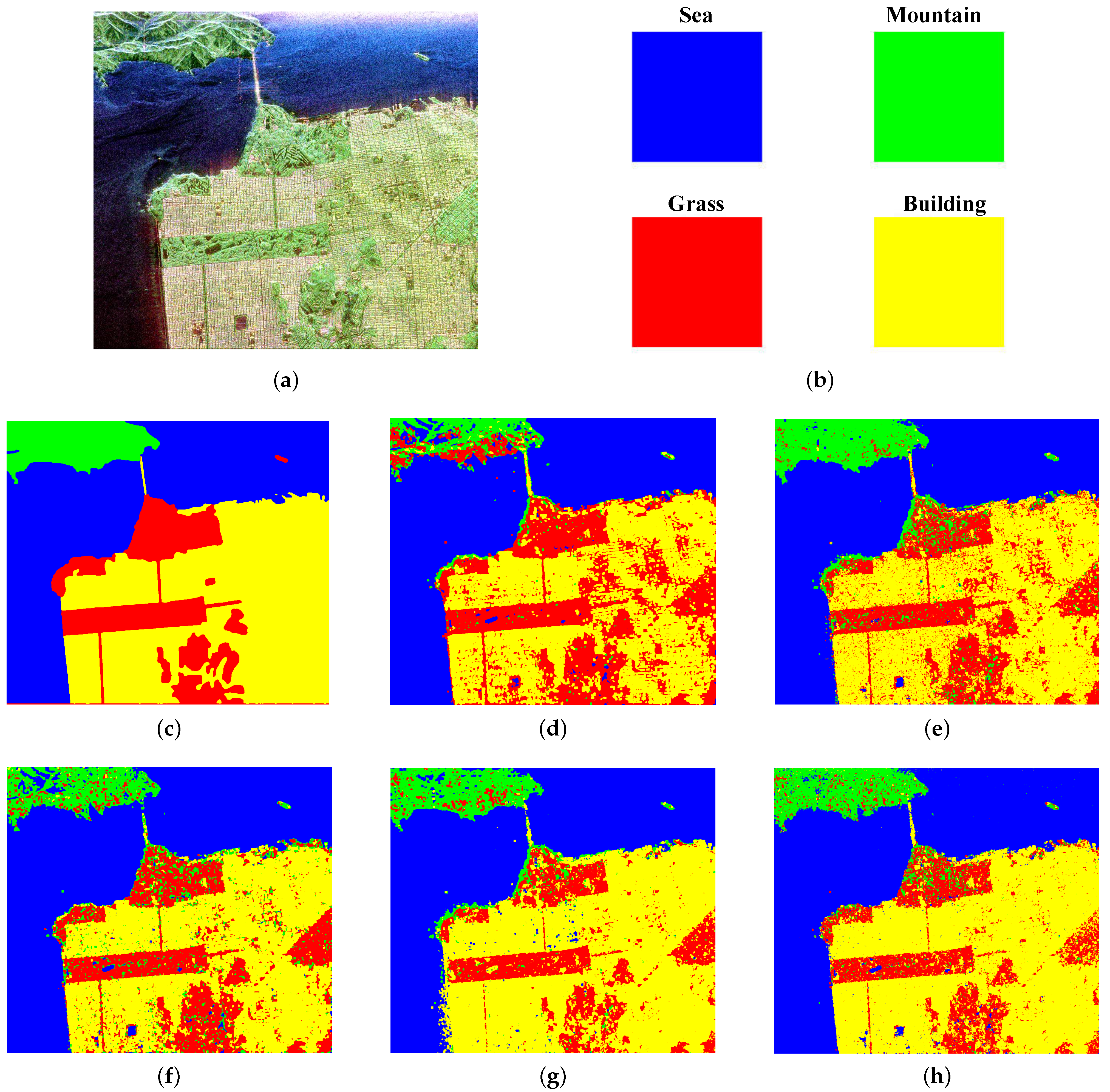
5.2.2. Evaluation on SanFransco

For the SanFransco image, the visual classification results of each algorithm are shown in Figure 7c–h and the classification accuracies are in Table 2. It can be seen clearly that all the methods worked better than on the Flevoland-1989 data due to the SanFransco image having fewer classes. Significantly, our method was also better than the others both regarding AC and kappa, except for LE-NDR.
As shown in Figure 7d–h, the sea which occupies half of the image was classified well with all methods, but the isle was classified wrong by all. From Figure 7d,f, the Wishart-ML method clearly mistakenly classified most of the land as mountains and the ND-KSVD method classified the Golden Gate Bridge badly. In Figure 7e, some line targets which are a boulevard in truth were wrongly labeled as urban buildings by RSC-SVM.
From Table 2, our GADDL achieved the second highest performance on the whole. Almost all algorithms could not distinguish the grass well, which can be seen on the right of the Figure 7d–h. Our GADDL got low accuracy for grass, which was probably due to the classification ability mainly relying only on target decomposition. LE-NDR is a method based on polarization target decomposition which relies on the prior knowledge of the designer. For the SanFransco dataset with a small number of categories, this method can easily obtain more discriminative features and achieve the best classification results. Compared with RSC-SVM, our GADDL is more robust to category imbalances. The category of “Mountain” (Table 2) only made up 6% of samples, which is a small sample category. Our method still achieved a higher classification accuracy than RSC-SVM by 14.1% in terms of OA.

5.2.3. Evaluation on Flevoland-1991

To further verify the performance of our method, experiments on another fully PolSAR image with a far more unbalanced number of categories were implemented. Given Table 3, our GADDL achieved the best performance. In our chosen region, the number of pixels for the two categories (i.e., Maize and Buildings) were only 378 and 961, accounting for only 0.48% and 1.21% of the image, respectively. The accuracy of the comparison method in these categories was significantly lower than that for other categories, especially ND-KSVD. However, our method can still achieve high accuracy. This also further shows that our method is robust to class imbalance.
The confusion matrices of the compared methods and GADDL are shown in Figure 8a–e. From the comparison of these confusion matrices, it can be seen that our GADDL can distinguish categories well, even the categories with small numbers of samples.

5.3. Computational Cost

We tested the performance and efficiency of GADDL and the compared methods on three datasets. The results of the test time and OA are summarized in Table 4. All the experiments were implemented using Matlab 2014b on a standard computer with I7 8700k CPU and 64 GB RAM. According to the comparison results, the performance and efficiency of each method had the same trends on the three datasets. For example, on the Flevoland-1991 dataset, Wishart-ML, LE-NDR and ND-KSVD were faster than ours, but the accuracy was lower. GADDL achieved 24.5%, 7.5% and 18.5% better speed, respectively. In the testing phase, GADDL was the same as RSC-SVM, but we still gained a 2.3% improvement. It can be concluded that our method achieved a good trade-off in terms of accuracy and efficiency.

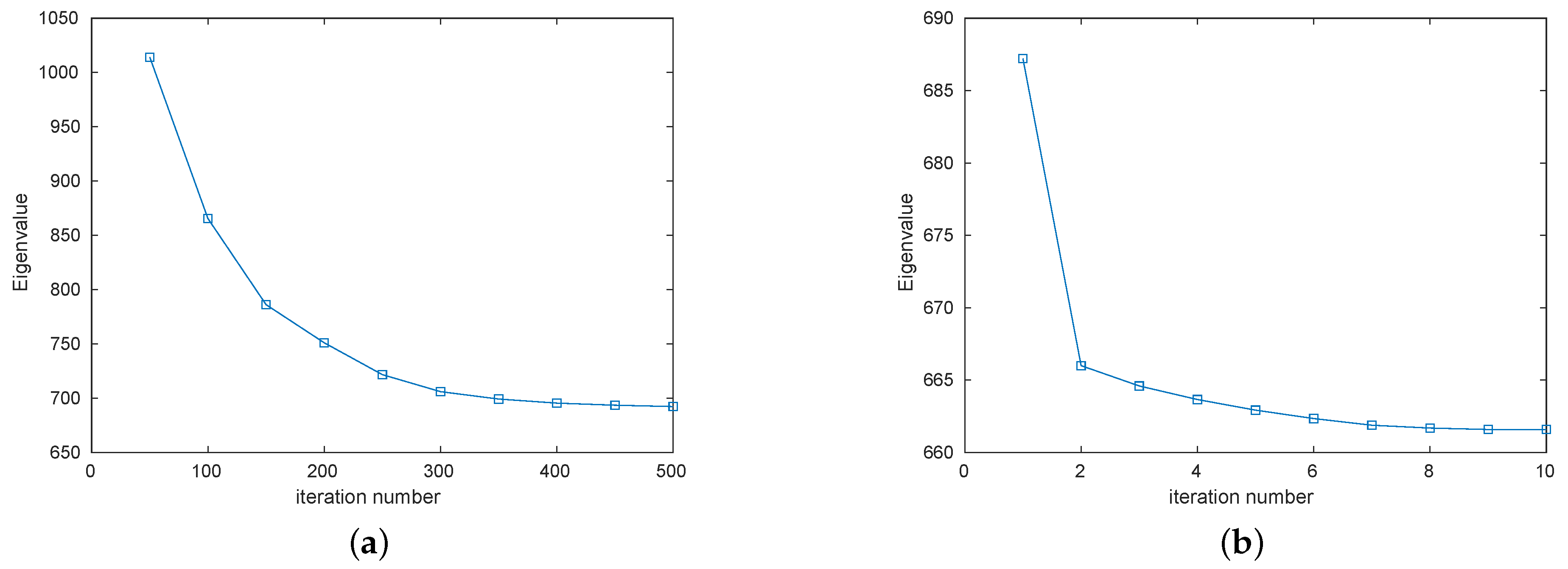
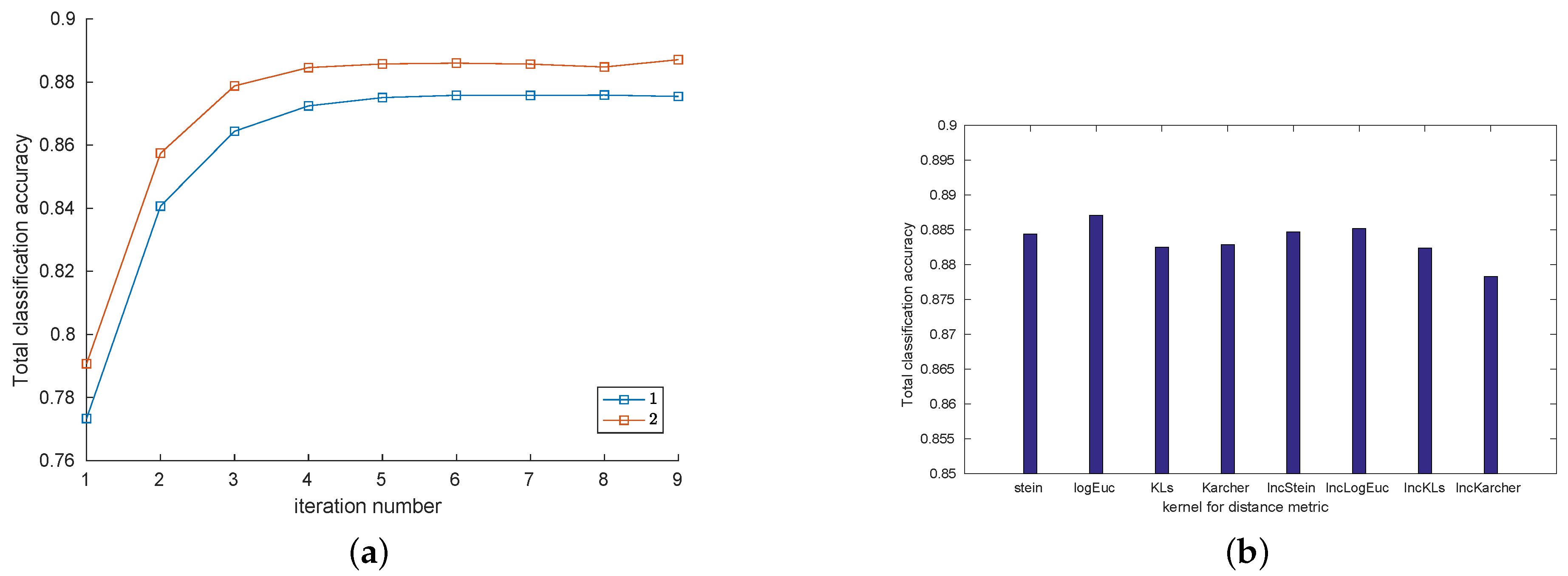
5.4. Convergence Analysis

The proposed GADDL is based on a sparse dictionary, which is used to illustrate the convergence by calculating the eigenvalue. We randomly selected 5% points for each type of Flevoland image; in all, 8203 matrices were used as experimental samples, and λ 1 , λ 2 , λ 3 and θ , represent 0.4 , 10 3 , 0.1 , 10 7 and 50 atoms respectively. We calculated the sum value of the reconstructed term, sparse regular term and discriminant term after each iteration. As can be seen from Figure 9, as the number of iterations increased, the curve decreased continuously and finally stayed nearly level.

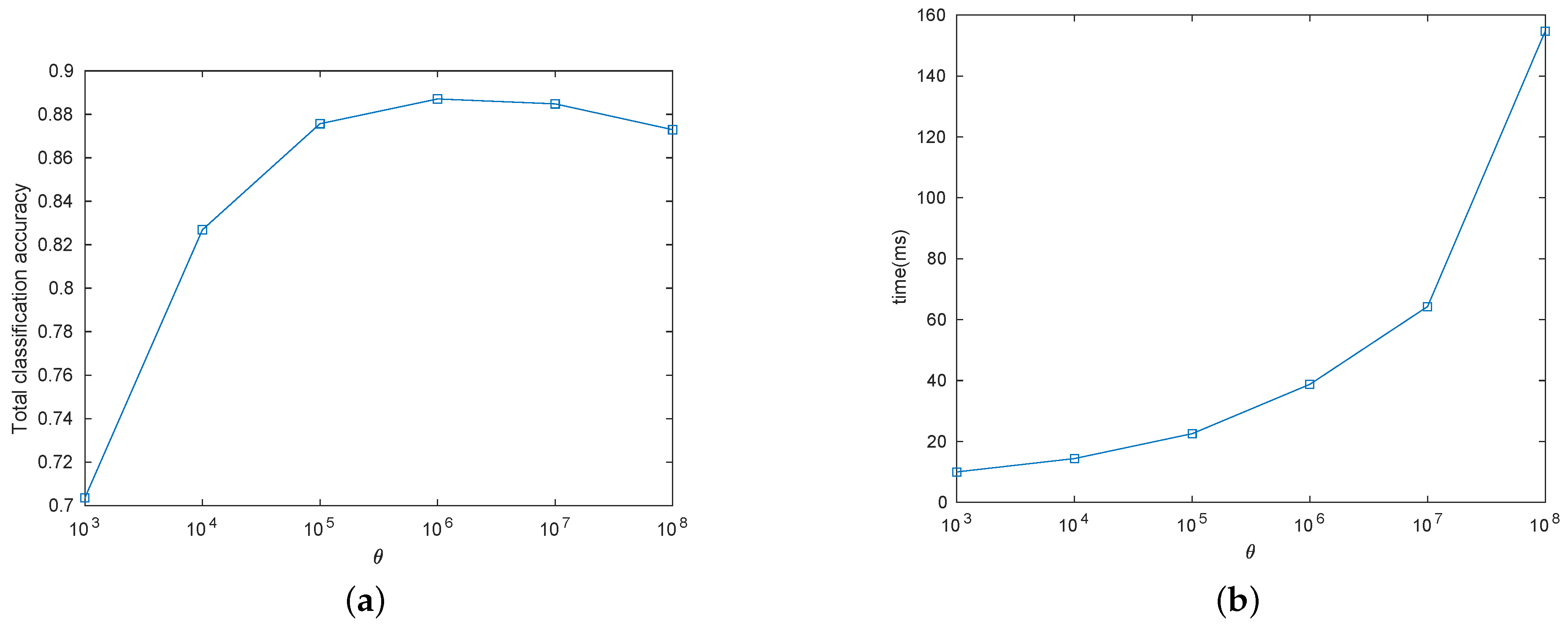
5.5. Parameter Analysis

In our method, there are several parameters closely related to the final results which need to be set, including the trade-off coefficients λ 1 , λ 2 and λ 3 related to the vector regular term, the discriminant term and the sparsity of dictionary, respectively. Moreover, the learning rate θ of the linear multi-svm classifier and the number of atoms for each type in dictionary are two key parameters. We conducted experiments in turn to prove the superiority of the selected parameters. The impacts assessed by comparing the total classification of the proposed method with different parameters are drawn out as curves for visualization.
According to the optimization strategy, the parameter θ , which stands for the learning rate of the classifier, is only used in the step optimizing W , b and has no effect on other parts of the experiment. From [34] we can find that with a decrease of the learning rate, the hyperplane obtained can be more suitable but more time consuming. We simply let θ be equal to a small value, 10 7 , which will be refined later. Then, the number of atoms for the dictionary for each type was first set as 30, which we decided by referring to other articles [18].
In general, due to the reconstructed terms and the regularized terms being the main parts of the dictionary learning, we first set λ 2 and λ 3 to relatively small values, such as 10 7 and 0.1 , respectively, to quantify the influences of different λ 1 . As shown in Figure 10, the weight coefficient of the vector of sparse constraint has a great influence on the final result. When λ 1 is set to between 0.1 and 1, we obtained better precision than for any other range. Furthermore, we changed the value of λ 1 from 0.1 to 1 with an interval of 0.1 to explore the influence on classification accuracy; the fluctuation of the resulting curve was less than 0.02. Then we set λ 1 to 0.4 in the experiments later.
Similarly, we performed experiments on the same data to investigate the impact of the parameter λ 2 , which is the weight coefficient of the discriminant term in the optimization target. It also is an important component of the Equation (20) optimizing z. As shown in Figure 11a, the value of λ 2 has a greater impact on the final accuracy. A value bigger than 10 5 makes the total classification accuracy lower; this may be caused due to an unbalanced contribution to the objective function. Additionally, a small value of λ 2 seems to lower the final result as well. To further verify the improvement of taking the discriminant term into consideration, we tried to set λ 2 to 0 fixing other parameters: the final precision was only 0.84; meanwhile, the highest precision was 0.86 as the value of λ 2 was set to 10 7 .
Furthermore, we implemented the same experiment to confirm the best value of parameter λ 3 . λ 3 is a parameter used to weigh the regularizer term of the dictionary tensor and constrain the sparsity of the dictionary, which can contribute to the gradient of dictionary in optimizing dictionary B . From Figure 11b, we can observe that the curve has a little fluctuation of within 0.01. In other words, the accuracy seems to make no difference with variable values of λ 3 . This may be because the initial dictionary obtained by clustering is better. It may also be attributed to the Riemann conjugate gradient method for direction and the line-search method for step-size. Therefore, the parameter λ 3 can be taken to be any integer from 1 to 0.001. We set it as 0.01 in the later experiments.
After that, we analyzed the influences of different numbers of dictionary atoms on the results. As we know, too small a size of the dictionary makes the model underfit, while a redundancy of dictionary atoms increases the computational burden. Thus, we need to set the size of the dictionary to as small as possible while the total classification accuracy is acceptable. In our experiment, the number of atoms for each class was set as the same value from 10 to 100 with an interval of 20 to observe a better balance between the dictionary size and the final accuracy. According to the experimental results shown in Figure 12, we found that when the number of dictionaries was set as about 50, the curve reached its peak value. However, considering the uneven distribution of the number of sample categories, the number of atoms in the dictionary for each class do not have to be the same. In this case, we assume that the number of atoms in the dictionary for a larger number of samples should be high, and vice versa. Therefore, we used the number of atoms of each type as 1 5 , 1 10 , 1 20 or 1 30 of the training data in each experiment, which showed higher accuracy in the same dataset in contrast to a similar dictionary size with an equal number of atoms for each class. We implemented the following experiment while setting the number of atoms to 1 10 of the training data to trade-off efficiency and precision.
Finally, we verified the optimal range of θ . θ is the learning rate when solving the optimal linear multi-SVM classification problem, which affects the balance between accuracy and time consumption. In our experiments, we had the parameter θ vary from 10 3 to 10 8 with average precision and time cost consumption. In Figure 13, we can see that the accuracy was almost the same when θ was bigger than 10 6 , and the time consumption increased in a geometrical progression. Meanwhile, when we set θ to 10 8 , the final results decreased a little. This may be explained that in this dataset, some classes such as water may have so few points that the classifier would overfit with a small θ . In conclusion, we can set θ = 10 7 for better performance and simplicity.

5.6. Robustness Analysis

For the optimization problem, the l 0 norm is impossible to calculate, and the l 1 norm, l 2 norm may have some different influences on the final result. We statistically analyze the effects of different norms in Figure 14a.
The objective function’s value with l 2 norm is generally half a point higher than the one with l 1 norm with the same parameters on the same datasets. The results using quadratic hinge loss were much better than those using squared loss, which further emphasizes the importance of the sparse weight matrix. Thus, we chose the l 2 norm regularizer in the later discussion due to its computational efficiency.
As a discriminant dictionary learning model, the initial dictionary is a vital subproblem. Although some effective but complex algorithms have been proposed to obtain an initial dictionary, we just applied the k-means algorithm and extended it to the Riemannian manifold to obtain cluster centers as dictionary atoms. However, the traditional k-means cluster method implemented on Euclidean space works badly on the HPD matrix dataset. Therefore, different distance metrics for the Riemannian manifold were proposed. Assume two SPD matrices, X , Y S + d ; for statistical measures, the log-determinant divergence has the following form: d B ( X , Y ) = T r ( X Y 1 ) l o g | X Y 1 | d . As for differential geometric schemes, one of the most popular is the log-Euclidean metric defined as d l e = L o g ( X ) L o g ( Y ) F . As for kernelized schemes, the Stein divergence is defined as d S ( X , Y ) = l o g | 1 2 ( X + Y ) | 1 2 l o g ( X Y ) . We simply replaced the distance metric in the k-means algorithm with the Riemannian metric to cluster center points for each class as the atoms of sub-dictionary, and then combined them to create our initial discriminant dictionary. In all, eight different distance calculation methods were used to prove the robustness of the proposed method. As shown in Figure 14b, the Riemannian metric achieved high values of classification accuracy. The range of difference in the classification accuracy with different initial dictionaries was less than 0.5 % , which is very small. Therefore, the proposed algorithm is robust for the different Riemannian metrics. Then, we used log-Euclidean in the following experiments.

6. Conclusions

In this paper, we propose a novel, geometry-aware discriminative dictionary learning framework for classifying land covers in PolSAR data. For each pixel in the PolSAR image being described as an HPD matrix, in contrast to traditional sparse coding approaches, which use extracted features from HPD matrices as atoms of a dictionary, we directly create the dictionary with an HPD matrix. The initial dictionaries are obtained utilizing k-means algorithm under the Riemannian metric, so that we obtain a list of nonnegative linear combinations of dictionaries for each point, which is named sparse coding. We first attempted to optimize the dictionary and match the large hyperplanes respectively, and then to obtain more suitable sparse coding. We repeat this step so that a more consummate model is generated. Experimental results on the real PolSAR datasets demonstrate that the proposed method outperforms many state-of-the-art methods in terms of accuracy and kappa.
The proposed algorithm also has limitations. As shown in the SanFransico dataset, the boundary between two labeled classes is not accurate. Additionally, for the correct division, some outliers need post-processing. Our randomly selected training data also contains some outliers, which damage the final average accuracy. In this case, we can improve the initial clustering method to reduce the impact.

Author Contributions

Y.Z. and X.L. developed the algorithm, performed the experiments, and wrote this manuscript. Y.X. outlined the research topic. Y.Q. make the optimization model and analyze the computational complexity. C.L. assisted with manuscript writing. All authors have read and agreed to the published version of the manuscript.

Funding

This research was funded by the National Natural Science Foundation of China under Grant 61876161, Grant 61772524, the National Key Research and Development Program of China No.2020AAA0108301, and Natural Science Foundation of Shanghai No.20ZR1417700.

Data Availability Statement

The data presented in this study are available on request from the corresponding author.

Conflicts of Interest

The authors declare no conflict of interest.

References

  1. Cloude, S.R.; Pottier, E. An entropy based classification scheme for land applications of polarimetric SAR. IEEE Trans. Geosci. Remote. Sens. 1997, 35, 68–78. [Google Scholar] [CrossRef]
  2. Yamaguchi, Y.; Moriyama, T.; Ishido, M.; Yamada, H. Four-component scattering model for polarimetric SAR image decomposition. IEEE Trans. Geosci. Remote. Sens. 2005, 43, 1699–1706. [Google Scholar] [CrossRef]
  3. Freeman, A.; Durden, S.L. A three-component scattering model for polarimetric SAR data. IEEE Trans. Geosci. Remote. Sens. 1998, 36, 963–973. [Google Scholar] [CrossRef] [Green Version]
  4. Pottier, E.; Saillard, J. On radar polarization target decomposition theorems with application to target classification, by using neural network method. In Proceedings of the 1991 Seventh International Conference on Antennas and Propagation, ICAP 91 (IEE), New York, NY, USA, 15–18 April 1991; pp. 265–268. [Google Scholar]
  5. Fukuda, S.; Hirosawa, H. Support vector machine classification of land cover: Application to polarimetric SAR data. In Proceedings of the IGARSS 2001. Scanning the Present and Resolving the Future. Proceedings. IEEE 2001 International Geoscience and Remote Sensing Symposium (Cat. No. 01CH37217), Sydney, NSW, Australia, 9–13 July 2001; Volume 1, pp. 187–189. [Google Scholar]
  6. Lardeux, C.; Frison, P.L.; Tison, C.; Souyris, J.C.; Stoll, B.; Fruneau, B.; Rudant, J.P. Support vector machine for multifrequency SAR polarimetric data classification. IEEE Trans. Geosci. Remote. Sens. 2009, 47, 4143–4152. [Google Scholar] [CrossRef]
  7. Ghoggali, N.; Melgani, F.; Bazi, Y. A multiobjective genetic SVM approach for classification problems with limited training samples. IEEE Trans. Geosci. Remote Sens. 2009, 47, 1707–1718. [Google Scholar] [CrossRef]
  8. She, X.; Yang, J.; Zhang, W. The boosting algorithm with application to polarimetric SAR image classification. In Proceedings of the 2007 1st Asian and Pacific Conference on Synthetic Aperture Radar, Huangshan, China, 5–9 November 2007; pp. 779–783. [Google Scholar]
  9. Zou, T.; Yang, W.; Dai, D.; Sun, H. Polarimetric SAR image classification using multifeatures combination and extremely randomized clustering forests. EURASIP J. Adv. Signal Process. 2009, 2010, 1–9. [Google Scholar] [CrossRef] [Green Version]
  10. Tannous, O.; Kasilingam, D. Independent component analysis of polarimetric SAR data for separating ground and vegetation components. In Proceedings of the 2009 IEEE International Geoscience and Remote Sensing Symposium, Cape Town, South Africa, 12–17 July 2009; Volume 4, pp. IV-93–IV-96. [Google Scholar]
  11. Wang, H.; Pi, Y.; Cao, Z. Unsupervised classification of polarimetric SAR images based on ICA. In Proceedings of the Third International Conference on Natural Computation (ICNC 2007), Haikou, China, 24–27 August 2007; Volume 3, pp. 576–582. [Google Scholar]
  12. Zhang, Y.D.; Wu, L.; Wei, G. A new classifier for polarimetric SAR images. Prog. Electromagn. Res. 2009, 94, 83–104. [Google Scholar] [CrossRef] [Green Version]
  13. Tu, S.T.; Chen, J.Y.; Yang, W.; Sun, H. Laplacian eigenmaps-based polarimetric dimensionality reduction for SAR image classification. IEEE Trans. Geosci. Remote. Sens. 2011, 50, 170–179. [Google Scholar] [CrossRef]
  14. He, C.; Li, S.; Liao, Z.; Liao, M. Texture Classification of PolSAR Data Based on Sparse Coding of Wavelet Polarization Textons. IEEE Trans. Geosci. Remote. Sens. 2013, 51, 4576–4590. [Google Scholar] [CrossRef]
  15. Zhang, L.; Sun, L.; Zou, B.; Moon, W.M. Fully Polarimetric SAR Image Classification via Sparse Representation and Polarimetric Features. IEEE J. Sel. Top. Appl. Earth Obs. Remote. Sens. 2015, 8, 3923–3932. [Google Scholar] [CrossRef]
  16. Xie, W.; Jiao, L.; Zhao, J. PolSAR Image Classification via D-KSVD and NSCT-Domain Features Extraction. IEEE Geosci. Remote. Sens. Lett. 2016, 13, 227–231. [Google Scholar] [CrossRef]
  17. Yang, F.; Gao, W.; Xu, B.; Yang, J. Multi-Frequency Polarimetric SAR Classification Based on Riemannian Manifold and Simultaneous Sparse Representation. Remote Sens. 2015, 7, 8469–8488. [Google Scholar] [CrossRef] [Green Version]
  18. Zhong, N.; Yan, T.; Yang, W.; Xia, G. A supervised classification approach for PolSAR images based on covariance matrix sparse coding. In Proceedings of the 2016 IEEE 13th International Conference on Signal Processing (ICSP), Chengdu, China, 6–10 November 2016; pp. 213–216. [Google Scholar] [CrossRef]
  19. Cai, S.; Zuo, W.; Zhang, L.; Feng, X.; Wang, P. Support Vector Guided Dictionary Learning. In Proceedings of the Computer Vision—ECCV 2014, Zurich, Switzerland, 6–12 September 2014; Fleet, D., Pajdla, T., Schiele, B., Tuytelaars, T., Eds.; Springer International Publishing: Cham, Switzerland, 2014; pp. 624–639. [Google Scholar]
  20. Cherian, A.; Sra, S. Riemannian Dictionary Learning and Sparse Coding for Positive Definite Matrices. IEEE Trans. Neural Networks Learn. Syst. 2017, 28, 2859–2871. [Google Scholar] [CrossRef] [Green Version]
  21. Birgin, E.G.; Raydan, M. SPG: Software for Convex-Constrained Optimization. Acm Trans. Math. Softw. 2001, 27, 340–349. [Google Scholar] [CrossRef]
  22. Hiai, F.; Petz, D. Riemannian metrics on positive definite matrices related to means. Linear Algebra Its Appl. 2012, 430, 3105–3130. [Google Scholar] [CrossRef] [Green Version]
  23. Absil, P.A.; Mahony, R.; Sepulchre, R. Optimization Algorithms on Matrix Manifolds:First-Order Geometry; Princeton University Press: Princeton, NJ, USA, 2009; pp. 17–51. [Google Scholar]
  24. Absil, P.A.; Baker, C.G.; Gallivan, K.A. Trust-Region Methods on Riemannian Manifolds. Found. Comput. Math. 2007, 7, 303–330. [Google Scholar] [CrossRef]
  25. Bertsekas, D.P. Nonlinear Programming. J. Oper. Res. Soc. 1997, 48, 334. [Google Scholar] [CrossRef]
  26. Yang, J.; Yu, K.; Gong, Y.; Huang, T. Linear spatial pyramid matching using sparse coding for image classification. In Proceedings of the 2009 IEEE Conference on Computer Vision and Pattern Recognition, Miami, FL, USA, 20–25 June 2009; pp. 1794–1801. [Google Scholar] [CrossRef] [Green Version]
  27. Schmidt, M.W.; Berg, E.V.D.; Friedlander, M.P.; Murphy, K.P. Optimizing Costly Functions with Simple Constraints: A Limited-Memory Projected Quasi-Newton Algorithm. Hansen. Int. 2009, 5, 355–357. [Google Scholar]
  28. He, C.; Deng, J.; Xu, L.; Li, S.; Duan, M.; Liao, M. A novel over-segmentation method for polarimetric SAR images classification. In Proceedings of the 2012 IEEE International Geoscience and Remote Sensing Symposium, Munich, Germany, 22–27 July 2012; pp. 4299–4302. [Google Scholar]
  29. Hoekman, D.H.; Vissers, M.A. A new polarimetric classification approach evaluated for agricultural crops. IEEE Trans. Geosci. Remote. Sens. 2003, 41, 2881–2889. [Google Scholar] [CrossRef] [Green Version]
  30. Xiao, D.; Liu, C.; Wang, Q.; Wang, C.; Zhang, X. PolSAR Image Classification Based on Dilated Convolution and Pixel-Refining Parallel Mapping network in the Complex Domain. arXiv 2019, arXiv:1909.10783. [Google Scholar]
  31. Lee, J.S.; Cloude, S.R.; Papathanassiou, K.P.; Grunes, M.R.; Woodhouse, I.H. Speckle filtering and coherence estimation of polarimetric SAR interferometry data for forest applications. Geosci. Remote. Sens. IEEE Trans. 2003, 41, 2254–2263. [Google Scholar]
  32. Du, L.J.; Lee, J.S. Polarimetric SAR image classification based on target decomposition theorem and complex Wishart distribution. In Proceedings of the IGARSS ’96. 1996 International Geoscience and Remote Sensing Symposium, Lincoln, NE, USA, 31 May 1996; Volume 1, pp. 439–441. [Google Scholar] [CrossRef]
  33. Hua, W.; Wang, S.; Zhao, Y.; Yue, B.; Guo, Y. Semi-supervised PolSAR Classification Based on Improved Tri-training. In Proceedings of the 2017 IEEE International Geoscience and Remote Sensing Symposium (IGARSS), Fort Worth, TX, USA, 23–28 July 2017; pp. 3937–3940. [Google Scholar] [CrossRef]
  34. Hearst, M.A.; Dumais, S.T.; Osuna, E.; Platt, J.; Scholkopf, B. Support vector machines. IEEE Intell. Syst. Their Appl. 1998, 13, 18–28. [Google Scholar] [CrossRef] [Green Version]
Figure 1. The framework of our method in the training phase.
Remotesensing 13 01218 g001
Figure 2. Experiment on simulated PolSAR data. (a) Eigenvalue while optimizing sparse coding z. (b) Eigenvalue while optimizing dictionary B .
Remotesensing 13 01218 g002
Figure 3. The Flevoland-1989 dataset. (a) Pauli RGB composite image. (b) Ground truth map.
Remotesensing 13 01218 g003
Figure 4. The San Francisco dataset. (a) Pauli RGB composite image. (b) Ground truth map.
Remotesensing 13 01218 g004
Figure 5. The Flevoland-1991 dataset. (a) The pseudo RGB image. (b) Ground truth map.
Remotesensing 13 01218 g005
Figure 6. AIRSAR L-band PolSAR image of Flevoland-1989. (a) Pauli RGB composite image for the original data. (b) Color code. (c) Ground truth map. (d) Result of the Wishart-ML method. (e) Result of the LE-NDR method. (f) Result of the ND-KSVD method. (g) Result of the RSC-SVM method. (h) Result of our method.
Remotesensing 13 01218 g006
Figure 7. AIRSAR L-band PolSAR image of SanFransco. (a) Pauli RGB composite image for the original data. (b) Color code. (c) Ground truth map. (d) Result of Wishart-ML method. (e) Result of LE-NDR method. (f) Result of ND-KSVD method. (g) Result of RSC-SVM method. (h) result of ours.
Remotesensing 13 01218 g007
Figure 8. Confusion matrixes of classification under different methods.
Remotesensing 13 01218 g008
Figure 9. The total eigenvalue of objective function with the iteration goes.
Remotesensing 13 01218 g009
Figure 10. Eigenvalue versus varying scale parameter λ 1 . (a) λ 1 varies from 0.01 to 100. (b) λ 1 varies from 0.1 to 1.
Remotesensing 13 01218 g010
Figure 11. Eigenvalue versus varying scale parameter λ 2 , λ 3 . (a) λ 2 varies from 1 to 10 12 . (b) λ 3 varies from 10 to 10 5 .
Remotesensing 13 01218 g011
Figure 12. Eigenvalue versus varying scale parameter atom number. (a) with the same atom number for each class. (b) with atom number in proportion for each class.
Remotesensing 13 01218 g012
Figure 13. Accuracy and time-consuming versus varying scale parameter θ . (a) precision. (b) time costing.
Remotesensing 13 01218 g013
Figure 14. Classification accuracy versus varying norms and distance metrics. (a) accuracy under different norm regularization. (b) total classification accuracy under different distance metrics.
Remotesensing 13 01218 g014
Table 1. The overall accuracy (OA), average accuracy (AA) and kappa coefficient values of different methods on Flevoland-1989 dataset. # Num. denotes the number of samples in each category.
Class# Num.Wishart-MLLE-NDRND-KSVDRSC-SVMGADDL
Water86711110.9655
Pea147980.69580.68560.25320.66290.7331
Bean80980.93890.78200.88590.95540.9481
Grass97060.69370.30910.28430.83070.8144
Beet98950.91780.84790.65710.87730.8152
Rape219670.94820.83200.56340.74270.8230
Forest226390.88550.94510.94180.91240.9616
Alfalfa136550.72160.693810.87990.93530.9129
Bare58880.59850.84920.95620.98010.9423
Wheat400300.51040.75490.89890.86860.9241
Potato164340.91710.83560.85560.83110.9069
OA0.75830.77350.74900.84830.8848
AA0.80250.77590.74330.87240.8861
Kappa0.72630.73880.70640.82580.8669
Table 2. The overall accuracy (OA), average accuracy (AA) and kappa coefficient values of different methods on the SanFransco image. # Num. denotes the number of samples of each category.
Class# Num.Wishart-MLLE-NDRND-KSVDRSC-SVMGADDL
Sea3525770.98140.98170.98870.98390.9871
Mountain634190.49290.82470.70520.68210.8231
Grass1331640.82140.65780.74410.58620.6689
Building3724400.75180.93150.81930.93850.9145
OA0.83190.90380.86540.88730.9005
AA0.76190.84890.81430.79770.8484
Kappa0.75310.85440.80120.84480.8491
Table 3. The overall accuracy (OA), average accuracy (AA) and kappa coefficient values of different methods on Flevoland-1991 dataset. # Num. denotes the number of samples of each category.
Class# Num.Wishart-MLLE-NDRND-KSVDRSC-SVMGADDL
Grass118900.60060.78280.58550.94430.9597
Onion114410.88400.53760.99630.9963
Potatoes141260.69980.97130.89730.94950.9864
Wheat150500.60930.94580.85460.96870.9764
Rapeseed1134510.99160.91690.96210.9912
Beet72390.21240.80330.64070.97630.9794
Barley16810.98640.95650.89950.98800.9948
Lucerne21290.95600.91250.83140.98220.9965
Maize9610.54820.53620.53900.85090.9156
Buildings3780.44290.00.00270.46520.5850
Roads25320.51100.43450.07860.54100.7048
OA0.72760.89680.78660.94980.9718
AA0.68790.74710.61670.87500.9078
Kappa0.72630.68640.74870.94100.9668
Table 4. The test time (minutes) of different methods on three datasets.
Datasets Wishart-MLLE-NDRND-KSVDRSC-SVMGADDL
Flevoland-1989Test-time9.1335.526.0883.4898.1
OA0.75830.77350.7490.84830.8848
SanFranscoTest-time20.71475.944.3986.01001.8
OA0.83190.90380.86540.88730.9005
Flevoland-1991Test-time7.1147.512.3428.4428.6
OA0.72760.89680.78660.94980.9718
Publisher’s Note: MDPI stays neutral with regard to jurisdictional claims in published maps and institutional affiliations.

