Article

Improved Mekong Basin Runoff Estimate and Its Error Characteristics Using Pure Remotely Sensed Data Products

1
School of Geodesy and Geomatics, Wuhan University, Wuhan 430079, China
2
Key Laboratory of Geophysical Geodesy, Ministry of Natural Resources, Wuhan 430079, China
3
Department of Civil, Environmental and Geodetic Engineering, Ohio State University, Columbus, OH 43210, USA
4
Core Faculty, Translational Data Analytics Institute, Ohio State University, Columbus, OH 43210, USA
5
Department of Land Surveying and Geo-informatics, The Hong Kong Polytechnic University, Hong Kong, China
6
Department of Geography, Hong Kong Baptist University, Hong Kong, China
*
Author to whom correspondence should be addressed.
Remote Sens. 2021, 13(5), 996; https://doi.org/10.3390/rs13050996
Submission received: 17 January 2021 / Revised: 16 February 2021 / Accepted: 2 March 2021 / Published: 5 March 2021
(This article belongs to the Section Remote Sensing in Geology, Geomorphology and Hydrology)

Abstract

:
Basin runoff is a quantity of river discharge per unit basin area monitored close to an estuary mouth, essential for providing information on the flooding and drought conditions of an entire river basin. Owing to a decreasing number of in situ monitoring stations since the late 1970s, basin runoff estimates using remote sensing have been advocated. Previous runoff estimates of the entire Mekong Basin calculated from the water balance equation were achieved through the hybrid use of remotely sensed and model-predicted data products. Nonetheless, these basin runoff estimates revealed a weak consistency with the in situ ones. To address this issue, we provide a newly improved estimate of the monthly Mekong Basin runoff by using the terrestrial water balance equation, purely based on remotely sensed water balance component data products. The remotely sensed water balance component data products used in this study included the satellite precipitation from the Tropical Rainfall Measuring Mission (TRMM), the satellite evapotranspiration from the Moderate Resolution Imaging Spectroradiometer (MODIS), and the inferred terrestrial water storage from the Gravity Recovery and Climate Experiment (GRACE). A comparison of our new estimate and previously published result against the in situ runoff indicated a marked improvement in terms of the Pearson’s correlation coefficient (PCC), reaching 0.836 (the new estimate) instead of 0.621 (the previously published result). When a three-month moving-average process was applied to each data product, our new estimate further reached a PCC of 0.932, along with the consistent improvement revealed from other evaluation metrics. Conducting an error analysis of the estimated mean monthly runoff for the entire data timespan, we found that the usage of different evapotranspiration data products had a substantial influence on the estimated runoff. This indicates that the choice of evapotranspiration data product is critical in the remotely sensed runoff estimation.

Graphical Abstract

1. Introduction

River discharge (RD) measured near an estuary mouth is one of the critical water balance components, expressing itself in terms of basin runoff (R) when it is divided by the basin surface area [1]. Continuous monitoring of RD is useful to provide information on flooding and drought conditions, in order to account for potential agricultural losses [2,3]. Unfortunately, insufficient financial budgets have resulted in a number of poorly documented station RD time series over the past four decades [4]. As a result, RD estimated from remotely sensed data products has great potential for supplementing ground measurements worldwide [5,6], highlighting the importance of this study.
At present, the RD (or R) estimated from remotely sensed data can be grouped into the following five categories:
(1).
Passively sensed gridded data products, such as the normalized difference vegetation index (NDVI), are directly correlated with the in situ water level (or RD) at a nearby gridded point via a linear regression [7,8,9,10,11]. This method is simple and common; however, these data products have no direct causal relationship with RD.
(2).
Both actively and passively sensed water balance component data products, such as precipitation (P) from the Tropical Rainfall Measuring Mission (TRMM) [12] (hereinafter denoted TRMM-P), evapotranspiration (ET) from the Moderate Resolution Imaging Spectroradiometer (MODIS) [13] (hereinafter denoted MODIS-ET), and terrestrial water storage (S) from the Gravity Recovery and Climate Experiment (GRACE) [14] (hereinafter denoted GRACE-S), are aggregated over the entire basin or sub-basin individually before being correlated with the water level [15] or R [16]. This method is similar to the first method, but the difference lies in the use of the aggregated remotely sensed water balance data over the entire basin or sub-basin.
(3).
Passively sensed river width is inputted into hydraulic functional models to estimate the RD (e.g., [17,18,19,20,21]). Despite elegant models, high-resolution remote sensing imagery and an accurate in situ measured roughness coefficient are required [22,23,24]. Hence, this method is still dependent on the in situ measurements, which is not desirable.
(4).
An actively sensed water level (or so-called stage) measured from satellite altimetry is directly correlated with nearby in situ RD either via rating curves (e.g., [25,26,27]) or an ensemble-learning regression technique [28]. This method is direct; however, the nominal size of the radar altimetric footprint (i.e., between 3.5 km and 5 km (e.g., [29])) is normally larger than the river width. This results in an inaccurately sensed water level because the reflected radar signal is contaminated by the riverside (e.g., [30]).
(5).
Based on the terrestrial or combined land–atmosphere water balance equation, R can be estimated using a combination of a remotely sensed water balance component (RSWBC) and model-predicted data products [31,32,33,34]. This method is independent of in situ measurements; however, R accuracy is highly dependent on reliable model-predicted data.
Among the five categories, only the last method can be truly independent of the in situ and model-predicted data, largely owing to the remotely sensed S obtained from GRACE since 2002.
GRACE is a satellite mission for observing global time-variable relative gravity, thereby inferring S anomalies with respect to the geoid (i.e., the equipotential surface of the gravity field) with about a three-arc degree gridded spatial resolution at a monthly scale (e.g., [14,35]). This remotely sensed S, which significantly complements the insufficient ground measurements, has gradually become an indispensable component for basin-scale RD or R estimates (e.g., [31,32,33]).
With regard to the combined land–atmosphere water balance equation (e.g., [36]), Syed et al. (2005) [32] first demonstrated its applicability for determining the monthly R estimates of the Amazon and Mississippi river basins by using GRACE-S and a modeled atmospheric moisture flux divergence from the National Centers for Environmental Protection–National Center for Atmospheric Research (NCEP-NCAR) and the European Centre for Medium-Range Forecasts (ECMWF). Similar studies were then conducted for large basins around the world, including the Mekong Basin [37]. The monthly R estimates for the Mekong Basin agree well with the in situ R, with a Pearson correlation coefficient (PCC) of 0.621, a root mean squares error (RMSE) of 46.144, and a Nash–Sutcliffe efficiency (NSE) of −0.521 (Figure 2 of [33]). Notably, GRACE-S were unavailable before 2003, and their change ( Δ S ) was assumed to be zero [38].
While the lack of GRACE-S data poses an unavoidable uncertainty, ET is another important source of errors for R estimates. Based on the terrestrial water balance equation, Ferreira et al. (2013) [31] estimated R for the Yangtze River Basin using TRMM-P, GRACE-S, and model-predicted ET from the Global Land Data Assimilation System (GLDAS) [39], while remotely sensed MODIS-ET data were used by Chen et al. (2019) [40]. The results of [40] showed better agreement with the in situ data because MODIS-ET data were generated using the Penman–Monteith equation, which is better adapted to cover types of croplands and grasslands than model-predicted ET from GLDAS in the Yangtze River Basin [13,41]. Nonetheless, both the MODIS-ET and GLDAS model-predicted ET should yield different results in different regions.
As a river basin stretching across different latitudes, the Mekong Basin (MB) is subject to a monsoonal climate and is particularly sensitive to seasonality. This basin is affected by the Indian Summer Monsoon, the Western North Pacific Summer Monsoon, and the East Asian Summer Monsoon [42], which intersect and interact with each other [43], as well as El Niño–Southern Oscillation (ENSO) influences [44]. Regardless of the upstream or downstream in the MB, the spatiotemporal pattern of P varies according to the above monsoon interactions, consequently causing the spatiotemporal redistribution of ET and S.
In addition, dams within the MB were actively constructed between 1990 and 2002 [45], owing to reasons of water security concerning different nations [46]. The substantial impact on RD for different seasons and years was quantitatively assessed using an RD time series before and after the dam constructions [47,48]. However, the annual change of RD was insignificant [45,48]. Note that as reliable RSWBC data were only available after 2002, in particular those of GRACE-S, the assessment of the RD change before and after 2002 could be safely avoided because the RSWBC data already recorded the distorted RD. Except for the study of monthly R estimates in the MB using the model-predicted atmospheric moisture flux divergence conducted by Syed et al. (2009) [33], no further study has been conducted.
Given the aforementioned reasons and potential error sources, this study aimed to improve R estimates of the MB based on pure RSWBC data that are truly independent of in situ and model-predicted data. Through the terrestrial water balance equation, the subtraction from among all the RSWBC data averaged over the entire basin should have also mitigated partial systematic effects due to dam operation and ENSO on the R estimates. The R estimates were subsequently compared to those published in [33] in order to demonstrate a marked improvement made in this study. Meanwhile, the mean monthly runoff performance was assessed in order to further explain potential reasons for discrepancies.
This study is organized into three sections: Section 2 presents the data and methodology applied, together with accuracy evaluation indicators; Section 3 presents and compares our estimated R values with a previous published result, along with discussion of the potential discrepancies for a particular RSWBC; and Section 4 summarizes and concludes our findings.

2. Data and Methods

All the remotely sensed data products and in situ datasets used in this study are summarized in Table 1. Notably, the remotely sensed TRMM-P (i.e., 0.25 ° × 0.25 ° ), the MODIS-ET (i.e., 0.5 ° × 0.5 ° ), and the GRACE-S (i.e., 1 ° × 1 ° or 3 ° × 3 ° ) data have different spatial resolutions (Table 1). Their differences are attributable to satellite mission purpose, orbit design, and active (i.e., point location sampling with its own light source) and/or passive (i.e., optical image sampling dependent on sunlight) remote sensing (see, e.g., [49]). Direct usage of these RSWBC data in the terrestrial water balance equation would result in rougher R estimates because the TRMM-P and MODIS-ET data have a higher resolution than those of GRACE-S. These RSWBC data ought to be unified to approximately the lowest spatial resolution before usage. Therefore, the TRMM and MODIS data were resampled at a 1 ° × 1 ° resolution, while the regular GRACE data were interpolated at a 1 ° × 1 ° resolution, through associated Legendre functions in spherical harmonics. Even when the RSWBC data were unified, we observed that further smoothing could further reduce the discrepancy between R estimates and in situ data.

2.1. River Discharge Data

The RD data time series were obtained from the Mekong River Commission (MRC). The Kratie station (latitude 12.48141o, longitude 106.01762o, elevation 26 m) was selected because it is situated ~500 km away from the estuary mouth (Figure 1), so the complexity due to the ocean tidal effect on the Mekong Delta (MD) [50] and the total adjustment effect from Tonle Sap Lake [51] are negligible. Therefore, the river discharge time series of Kratie station was chosen for assessing the performance of the estimated R values in this study.
Considering the potential instability of observations due to satellite orbit adjustment during the launch in 2002 and more missing data at the end of the mission phase during 2013–2015, GRACE-S covering the time span from 2003–2012 was used. Moreover, ENSO variability at various intensities distorting monsoons in the period from 2003–2012 caused the distortion of RSWBC data, and hence the R estimates, to a certain extent. This further helped in assessing the performance of our methodology and identifying error sources and characteristics of the RSWBC data under external variability. Hence, the 10-year time span between 2003 and 2012 was employed.
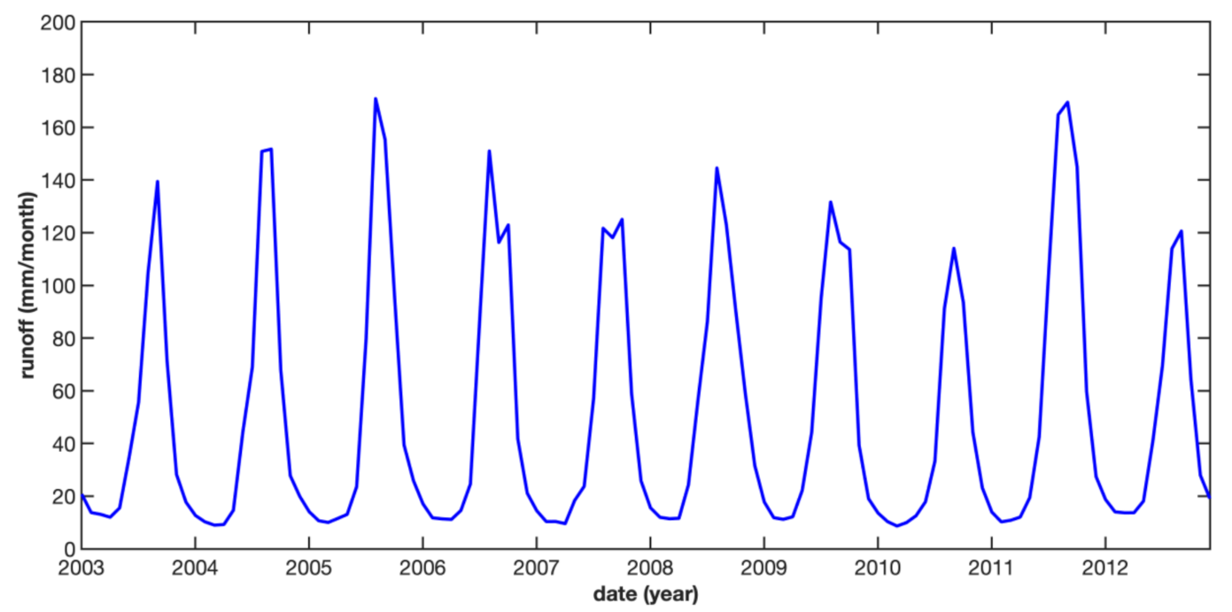
To be consistent with the monthly RSWBC data, the daily RD was transformed into a monthly R by applying a monthly data average divided by the MB surface area down to Kratie station (i.e., 646,000 km2). The runoff time series of Kratie station display a clear seasonal fluctuation pattern during the period from 2003–2012, with troughs relatively flatter and smoother than peaks (Figure 2). The yearly peaks and troughs appeared in September and April, respectively. This is because the rainfall season is between May and October and is controlled by the Southwest monsoon from the Indian Ocean, while the drought season is between November and April and is influenced by the northeast monsoon from the mainland [52]. The difference in peak values can be potentially attributed to irregular dam operations deployed to reduce the flooding conditions along the MB during the summer, in addition to ENSO variability [44].

2.2. Water Balance Gridded Data Products

The monthly quarter-degree gridded P data from the TRMM 3B43 version 7 [53] (i.e., TRMM-P; available at https://disc.gsfc.nasa.gov/datasets/TRMM_3B43_V7/summary, accessed on 16 January 2021) with a near-global coverage were used. Though parts of these datasets were bias-corrected with the Global Precipitation Climatology Centre (GPCP) gauges [54], their accuracy has not yet been confirmed.
The monthly half-degree gridded ET data from the MODIS MOD16A2 (i.e., MODIS-ET), estimated using the improved Penman–Monteith algorithm, were used [55]. This dataset has been made available by the University of Montana (http://www.ntsg.umt.edu/project/modis/, accessed on 16 January 2021). In addition, the GLDAS model-predicted ET generated from the Common Land Model (CLM) were used (available at https://disc.sci.gsfc.nasa.gov/datasets?keywords=GLDAS, accessed on 16 January 2021).
The monthly time-variable gravity data from GRACE enabled a conversion into globally gridded S data (i.e., GRACE-S). The regular release (RL) 05 and 06 (hereinafter abbreviated RL05 and RL06) and mascon solutions generated by the Center for Space Research (CSR) were used. Though the monthly gridded RL06 mascon data (http://www2.csr.utexas.edu/grace/RL06_mascons.html, accessed on 16 January 2021) at a 1 ° × 1 ° resolution could have been used directly, the RL05 and RL06 datasets (http://icgem.gfz-potsdam.de/series, accessed on 16 January 2021) were provided in terms of gravity Stokes coefficients (GSCs) up to the degree of 60, which is equivalent to a spatial resolution of about three arc degrees. Post-processing steps were necessary for the RL05 and RL06 data, including adding the degree-1 term and replacing the second zonal coefficient, C20, of the GSCs to account for the improved geocenter motion and the geoid, respectively [56,57]. De-striping and Gaussian filtering (with a 350-km radius) were applied to mitigate correlated noise in space [58]. Subsequently, the monthly gridded S time series were obtained using Equation (14) in [59] divided by the water density.
The monthly one-degree gridded S data were generated from the GLDAS soil moisture data [39], which are the sum of 0–10, 10–40, 40–100, and 100–200 cm layers. Four land-surface models, including the Common Land Model, Mosaic model, variable infiltration capacity (VIC) model, and the Noah model [39], were used.
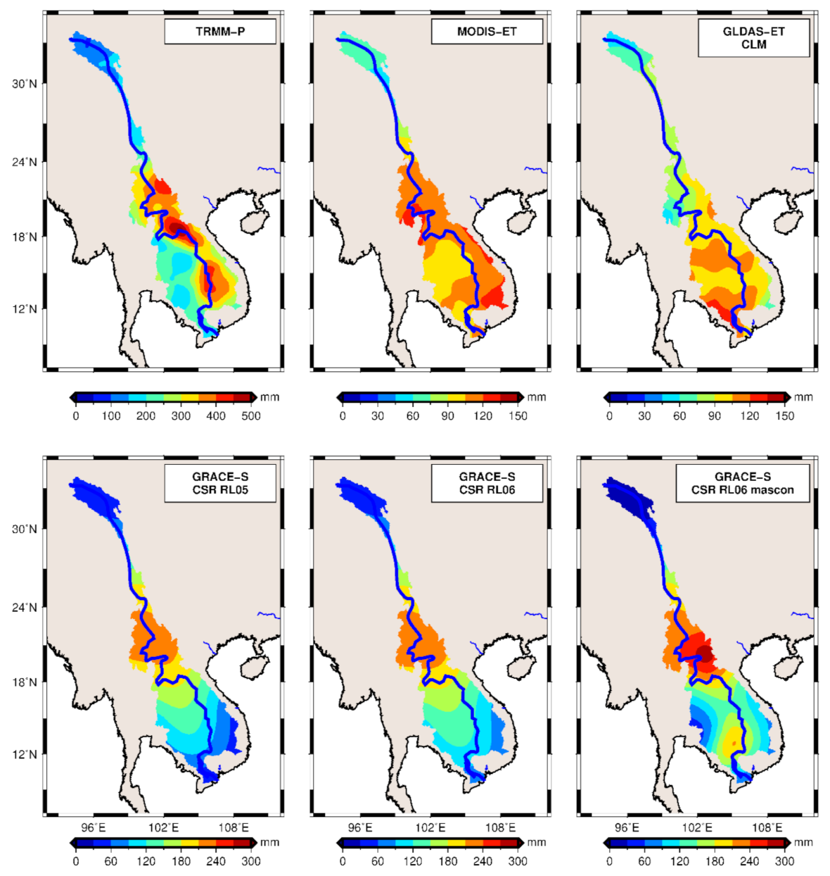
While both remotely sensed precipitation and evapotranspiration data have been compared with in situ data previously [40,41,60], remotely sensed water storage data could only be compared to the model-predicted water storage data (i.e., GLDAS models) due to the lack of in situ water storage measurements. All the above water balance gridded data products were visualized for a specific month in Summer (i.e., August 2008) in the MB (Figure 3), revealing the spatial heterogeneities of all RSWBCs. For instance, both TRMM-P and MODIS-ET presented larger values in the east of the main river channel than in the west. However, the GLDAS CLM-ET yielded a different spatial pattern when compared to MODIS-ET. All GRACE-S data presented similar patterns, except for the downstream MB for the GRACE mascon solution. These spatial heterogeneities potentially yield high uncertainties in R estimates when subtraction among RSWBCs through the terrestrial water balance equation, as is further discussed in Section 3.

2.3. Methodology

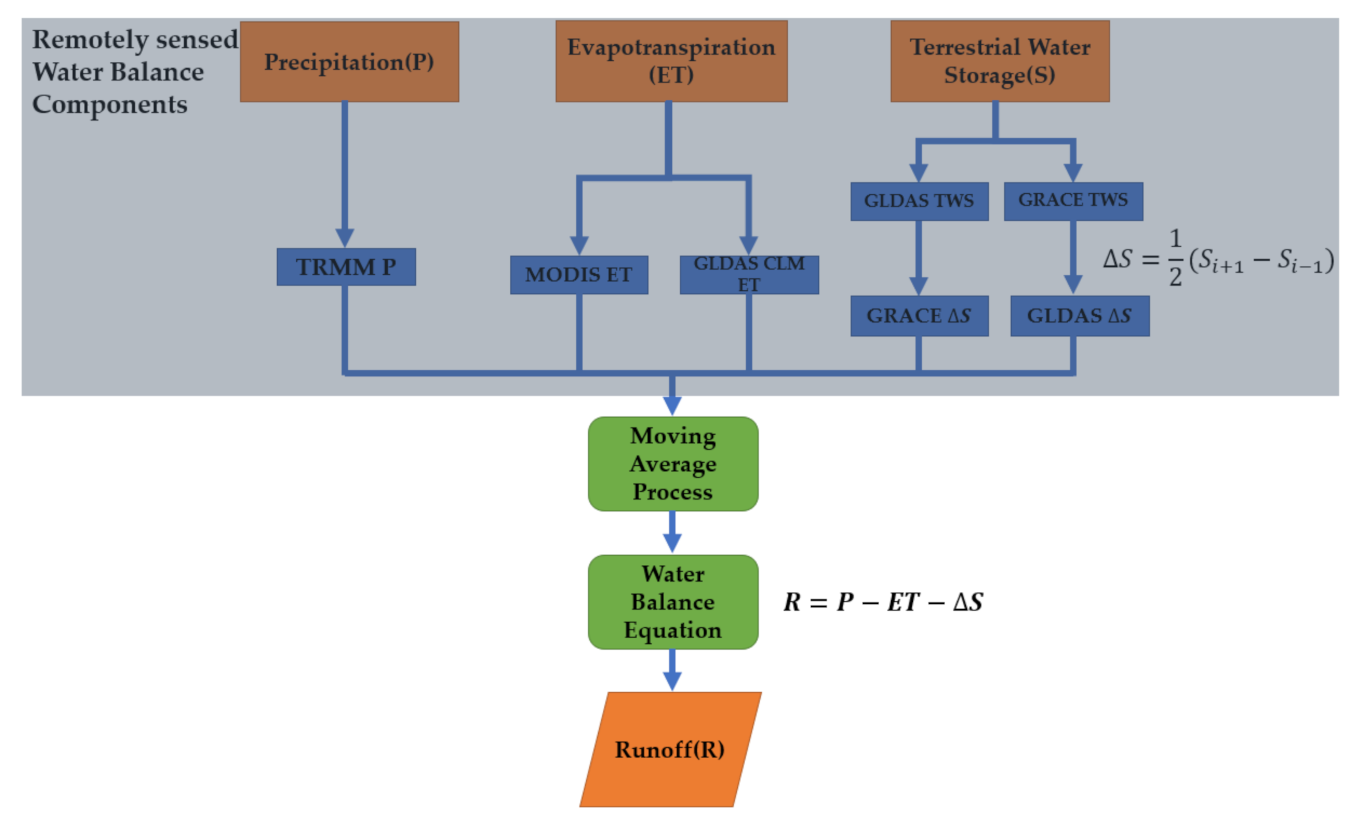
The remotely sensed basin runoff, R, for the MB bounded area up to Kratie station was determined from the terrestrial water balance equation [61] (Figure 4) as
R = P E T Δ S
where P, ET and ∆S are the precipitation, evapotranspiration, and the change of terrestrial water storage (in terms of mm/month), respectively. The change of terrestrial water storage in Equation (1) was defined in the following form:
Δ S = 1 2 S i + 1 S i 1
where S i is the terrestrial water storage anomaly with respect to the geoid of month i. Note again that the RSWBC data products were presented with different spatial resolutions, as stated above. These gridded data products were unified to a 1 ° × 1 ° resolution.
Gridded values of each data product within the MB were spatially summed up individually within the MB bounded area up to Kratie station (see Figure 1) each month to form a monthly time series for the period from 2003–2012. Due to the spatial heterogeneities for all RSWBCs within the entire MB, rougher R estimates generated from Equation (1) were obtained, and hence, further smoothing of the R estimates was required. Three-month, five-month, and seven-month moving averages were applied and compared against the in situ data. It was found that the three-month moving average was the best, because the five-month and seven-month moving averages caused a time-shift in the R estimates, resulting in larger discrepancies with the in situ data.

2.4. Accuracy Evaluation Indicators

The estimated time series of remotely sensed R in the MB were subjected to accuracy evaluation against the in situ R obtained from the Kratie station. Consistent with the accuracy evaluation indicators employed in classical and operational hydrology, the Pearson correlation coefficient, the Nash–Sutcliffe efficiency model coefficient, and the root mean square error and its normalized form (NRMSE) are conventional assessment indicators (as in, e.g., [62,63]). The mean absolute percentage error (MAPE) was also employed.
PCC, with its value within ± 1, measures the strength of collinearity between two variables. It is formulated as
P C C = i = 1 N R 0 i R 0 ¯ R m i R m ¯ N i = 1 N R 0 i R 0 ¯ 2 N i = 1 N R m i R m ¯ 2 N .
Commonly employed in the field of hydrology, the NSE model coefficient, with its value ranging between −∞ and 1, yields the efficient gain in the performance of the estimated R against the in situ R time series [64]. The best performance is achieved when the NSE equals one. It is formulated as
N S E = 1 i = 1 N R m i R 0 i 2 i = 1 N R 0 i R 0 ¯ 2
The RMSE is another commonly employed evaluation indicator for comparison of the estimated quantity against the in situ one. It is formulated as
R M S E = 1 N i = 1 N R m i R 0 i 2
The NRMSE is a normalized version of the RMSE, yielding a relative RMSE. It is defined as
N R M S E = 1 N i = 1 N R m i R 0 i 2 max R 0 i min R 0 i
The MAPE represents the average of the absolute error in terms of a fraction [65], calculated as:
M A P E = 1 N i = 1 N R 0 i R m i R 0 i
where R 0 i and R m i Ymare the in situ and remotely-sensed R values for each month i; R 0 ¯ and R m ¯ are the mean of R 0 i and R m i ; and max R 0 i and min R 0 i are the maximum and the minimum of the in situ R, respectively.

3. Results and Discussion

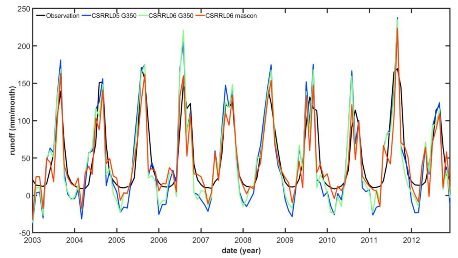
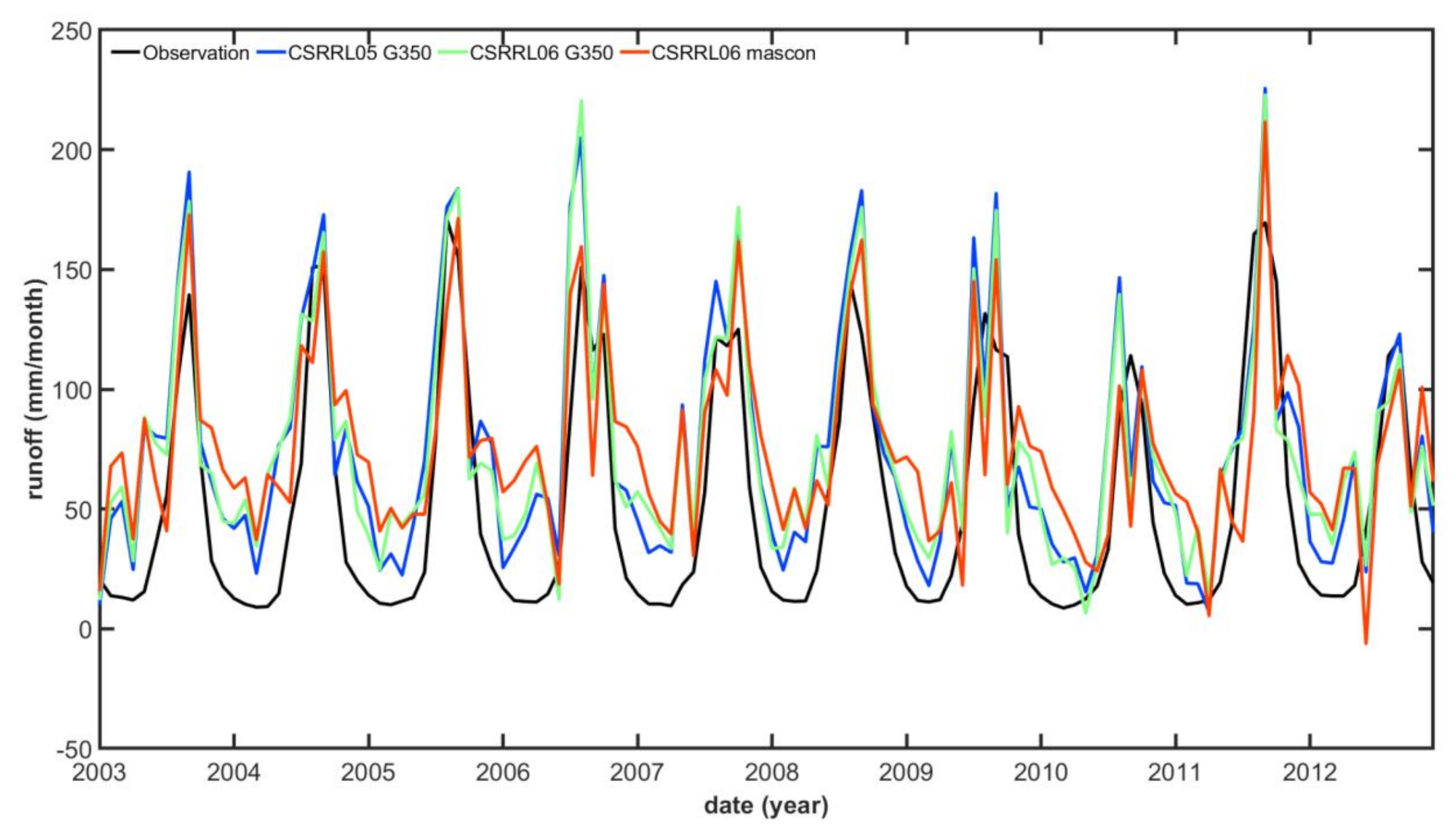
The R estimates (Figure 5) based purely on RSWBCs (namely TRMM-P, MODIS-ET, and several versions of GRACE-S) were compared with a combination of remotely sensed and modeled data products (namely GLDAS CLM-ET and several versions of GRACE-S, and MODIS-ET and several versions of GLDAS model-predicted S) (Figure 6 and Figure 7), using the same TRMM-P data (Table 2). Our analysis indicated that the R estimates based purely on RSWBCs yielded better results than the combination of remotely sensed and modeled data products. No matter the data products, all the estimated R values from these combinations yielded significantly higher PCCs, RMSEs, and NSEs than those of [33] (PCC of 0.621, RMSE of 46.144 mm/month, and NSE of −0.521). The best-estimated R at Kratie station, based purely on RSWBCs (i.e., MODIS-ET and GRACE-S CSR Mascon), resulted in a PCC of 0.836, RMSE (NRMSE) of 27.465 mm/month (0.169), and NSE of 0.665. A similar situation applied to other evaluation metrics in terms of ranking among different estimations of R. By evaluating the best-estimated R in terms of PCC, we were able to show a remarkable improvement when compared to the PCC of 0.621 obtained in [33].
Despite the remarkable improvement, all the R estimates were not as smooth as the in situ runoff, in particular the peaks and troughs. We observed a consistent discrepancy in troughs during dry seasons when compared to the in situ runoff. Using MODIS-ET and different GRACE-S data products, the R estimates showed an underestimation of the runoff during the dry seasons (Figure 5), while the one based on the CLM-ET yielded an overestimation (Figure 6). This highlights the unreliability of ET during the dry seasons, irrespective of whether observed or model-predicted ET data was used. As mentioned, GLDAS CLM-ET has a different spatial pattern from MODIS-ET, in addition to their differing magnitudes (Figure 3). As a result, ET can be one of the main error sources.
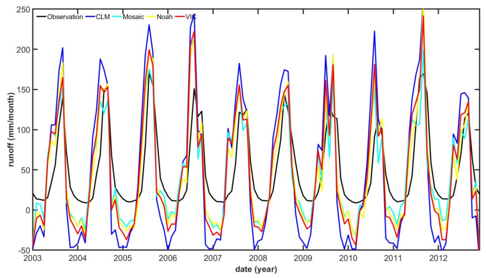
Employing MODIS-ET and several types of GLDAS model-predicted S data, the R estimates showed an underestimation (or overestimation) of the runoff during the dry (respectively, wet) seasons when compared to the in situ runoff (Figure 7). This indicates that the GLDAS model-predicted changes of terrestrial water storage (i.e., Δ S ) are always overestimated (underestimated) during the dry (wet) seasons. Moreover, variable time lag between the R estimates and the in situ runoff was present during the time period. These predicted changes in terrestrial water storage imply unrealistic terrestrial water storage conditions generated from GLDAS. This is the reason why the R estimates from MODIS-ET and different GRACE-S data products were better when compared against the in situ runoff (Table 2).
Overall, the in situ runoff presented a smaller range of fluctuations than our estimates. This is attributable to the result of the operation of cascaded dams covering the entire MB, which increases (or decreases) the runoff during drought (respectively, flooding) seasons with nearly no annual change (see, e.g., [45,66]). As a result, the in situ runoff presented smoother troughs than peaks. We speculate that the dam operations are not managed well during summer.
Note also that the runoff time series presents alternately high and low peak levels during 2010–2012, when El Niño and La Niña events occurred alternately with moderate intensities (https://ggweather.com/enso/oni.htm, accessed on 16 January 2021). This intensified the abnormal ranges of the precipitation and evapotranspiration, in addition to their spatiotemporal variations, and hence caused a larger runoff during the 2011 summer. This increased the discrepancy in peaks between the R estimates and the in situ R.
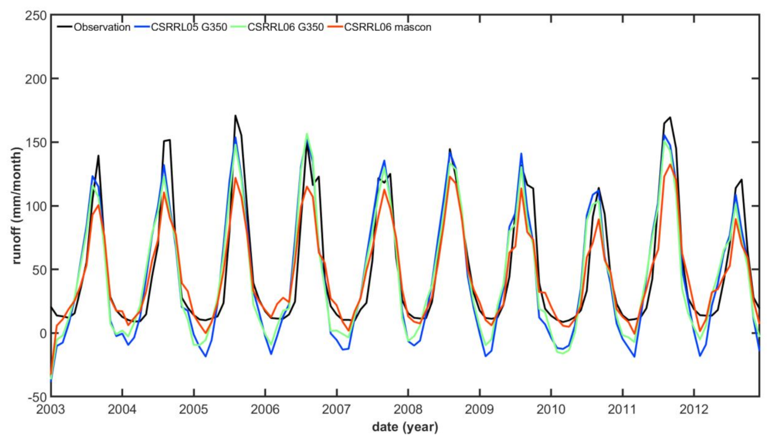
To mitigate the external influences due to climate variability, such as ENSO, on the R estimates, a three-month moving average was further applied to each RSWBC before R estimation using Equation (1), as mentioned. It can be seen that all estimated R values in this study were further improved, with the PCC of the best estimated R based purely on RSWBCs increasing from 0.836 to 0.932 (Table 2). This was mainly owing to the reduction of the discrepancy against the in situ R during dry seasons and for the peak during 2011 (Figure 8).
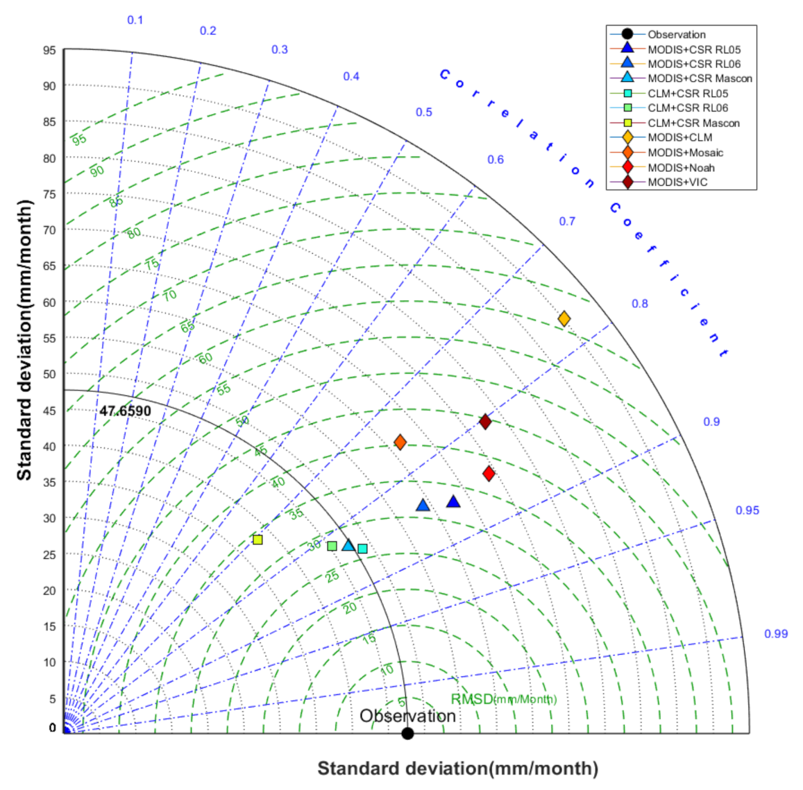
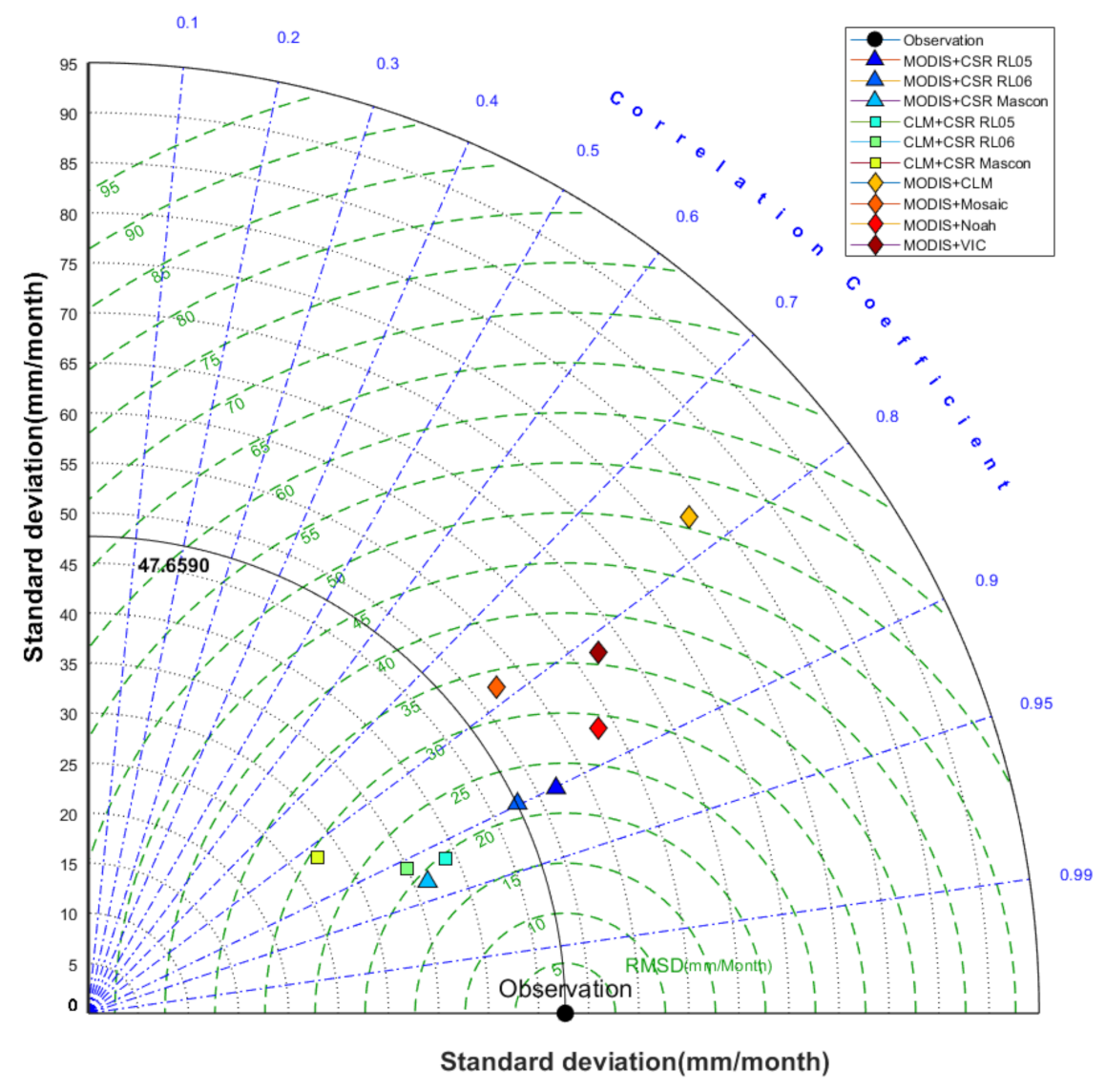
To further understand the error characteristics among the estimated R values from different data combinations, Taylor’s diagram was employed to visualize the correlation coefficient, the RMS difference (RMSD), and the standard deviation between the estimated and in situ values of R in a quarter pie chart [67]. Notice that the RMSD considers the mean offset between the estimated and in situ runoff, which is different from the RMSE. Figure 9 displays the accuracy evaluation statistics of the estimated R values derived through MODIS-ET with several versions of GRACE-S; GLDAS CLM-ET with several versions of GRACE-S; and MODIS-ET with several versions of GLDAS model-predicted S, against the in situ R. The estimated R values generated from MODIS-ET with several versions of GRACE-S were comparable to that generated from GLDAS CLM-ET with several versions of GRACE-S, contrary to the RMSE (Table 2). In addition, large discrepancies between the estimated R values generated by the GLDAS model-predicted S and the in situ R indicate that the GLDAS model-predicted S data products are not suitable for runoff estimation when compared to GRACE. After applying the three-month average for each data product before estimation, further improvement was achieved for all the estimated R values (Figure 10).
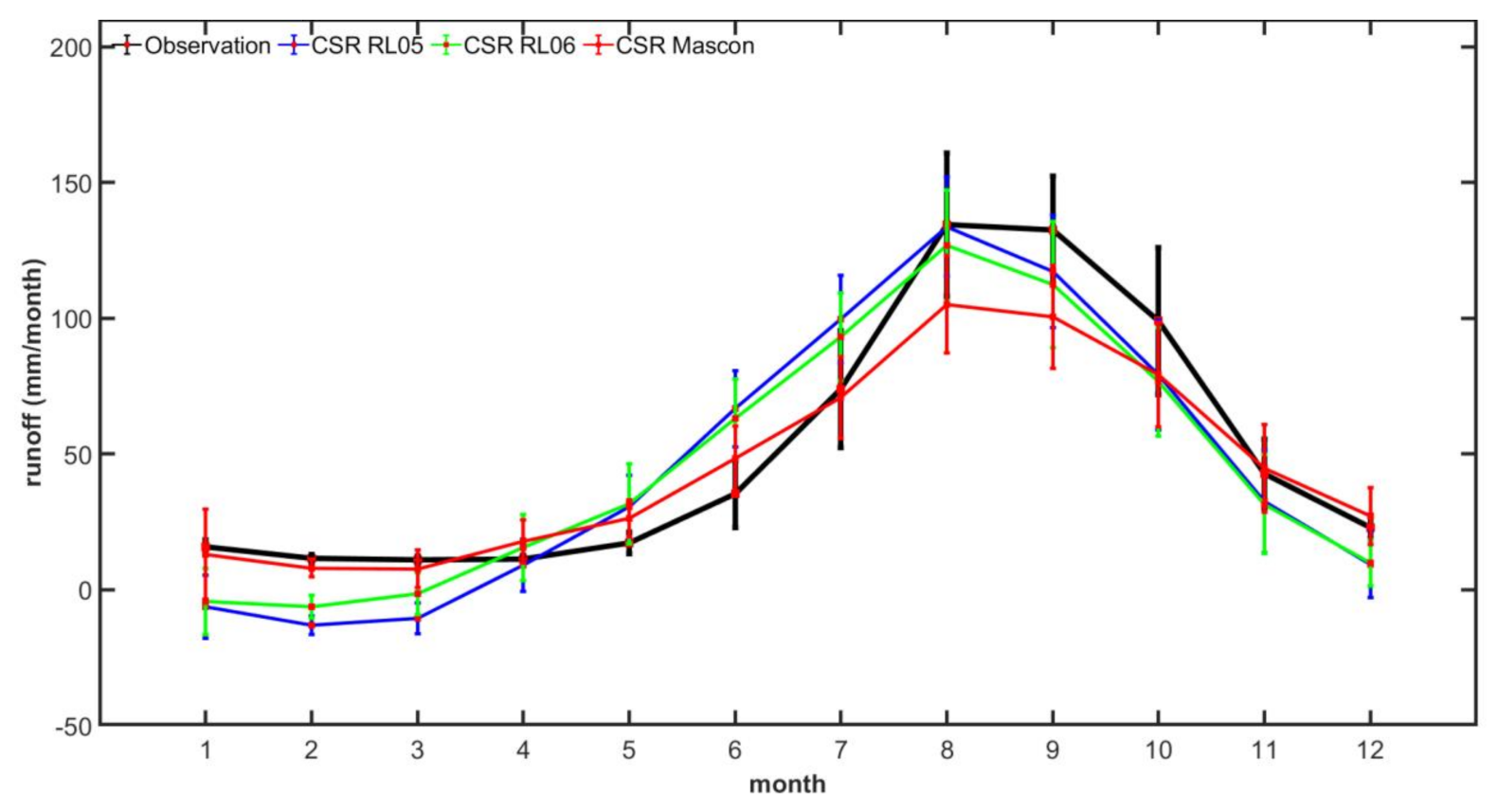
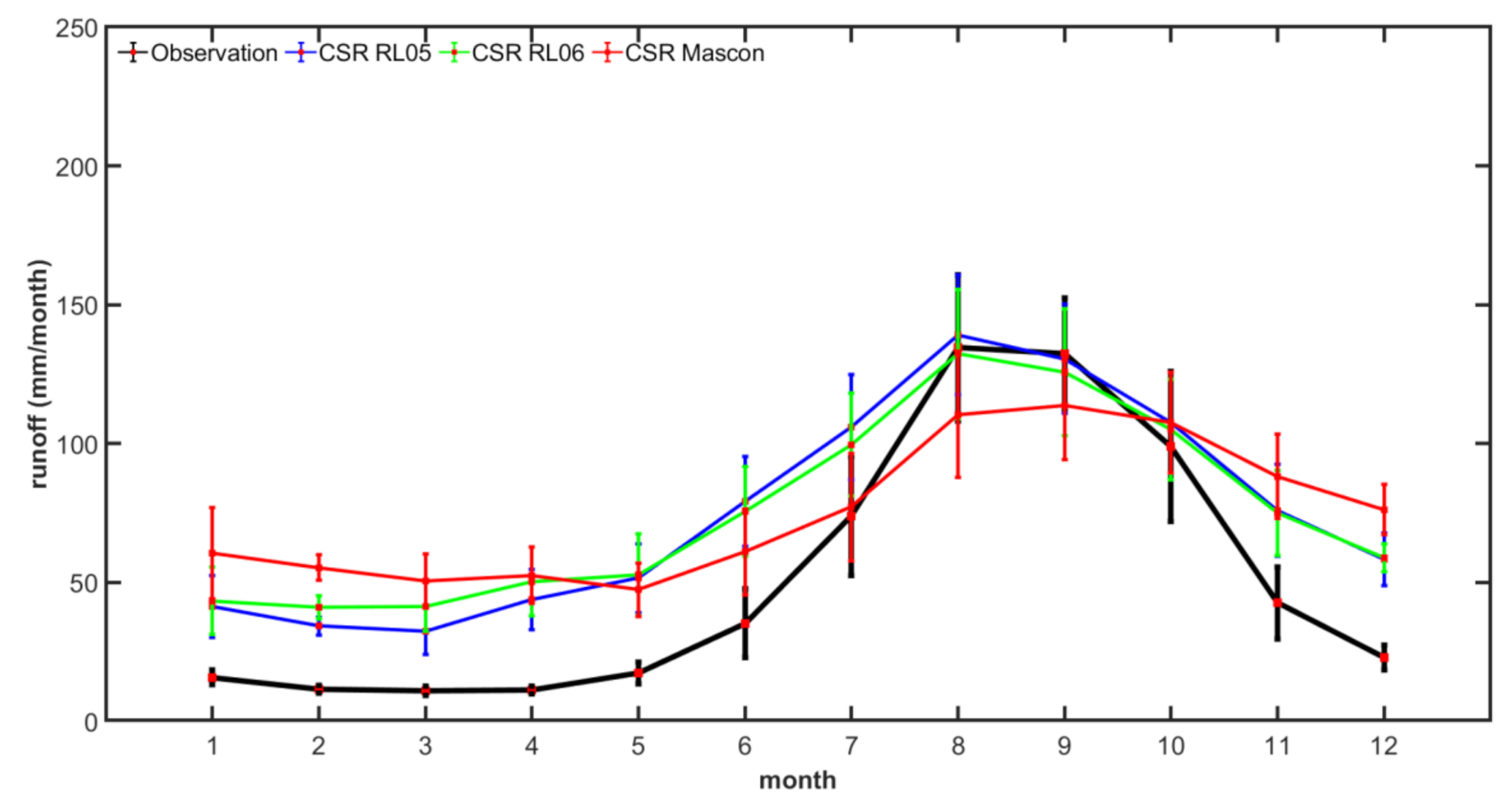
To further examine whether ET was influential on the estimated R values or not, the discrepancy between the estimated R values and the in situ runoff was evaluated with the estimated mean monthly R for MODIS-ET with several versions of GRACE-S and for GLDAS CLM-ET with several versions of GRACE-S, after applying a three-month average for each data product (Figure 11 and Figure 12). Comparing the mean monthly R values between the two dataset combinations, substantial differences can be observed (Figure 11 and Figure 12). Though the resulting R generated purely from the RSWBCs best matched the in situ R, the estimated mean monthly R presented various degrees of discrepancies for different seasons.
Apparently, the estimated mean monthly R for MODIS-ET with the GRACE CSR mascon was inconsistent with that of CSR RL05 and RL06 for the two dataset combinations (Figure 11 and Figure 12) because of the different data pre-processing strategies of RL05 (or RL06) and the mascon solutions. In the case of MODIS-ET with CSR mascon, the estimated mean monthly R was consistent with the in situ R for most months, except for being underestimated in August, September, and October (Figure 11). However, in the case of MODIS-ET with GRACE RL05 and RL06, the estimated mean monthly R values were underestimated (or overestimated) between September and March (respectively, May and July). As for the case of GLDAS CLM-ET with the CSR mascon, the estimated R was overestimated for all months except August and September (Figure 12). In the case of GLDAS CLM-ET with CSR RL05 and RL06, the estimated mean monthly R was overestimated for most months of the year, except for being matched well in August and September. Overall, the estimated mean monthly R generated from MODIS-ET with the CSR mascon exhibited smaller discrepancies than those from GLDAS CLM-ET with the CSR mascon. No matter whether MODIS-ET or GLDAS CLM-ET was used, unavoidable uncertainties arose during the remotely sensed R estimation process. After all, a number of research studies have complained about the uncertainty of ET data products at global or regional scales (e.g., [68,69]).

4. Summary and Conclusions

Previous study estimated the monthly runoff in the Mekong Basin according to the water balance equation, based on a hybrid use of the remotely sensed water balance component and modeled data products. In this study, we estimated the runoff purely using the RSWBC. After applying a three-month moving average to the RSWBCs, the best runoff estimate yielded a PCC of 0.932 when compared to the in situ runoff. This was a remarkable improvement when compared to the PCC of 0.621 obtained by Syed et al. (2009) [33]. We also found that dam operations and ENSO had a substantial impact on the R estimates when compared against the in situ runoff.
To further examine the error characteristics, we computed and compared the estimated mean monthly runoff. We found that, given the same TRMM precipitation and GRACE terrestrial water storage data, our best runoff estimate obtained purely from the RSWBCs was consistent with the in situ runoff for most months, whereas the runoff estimate based on GLDAS CLM evapotranspiration overestimated the runoff for most months. This finding indicates that the use of different ET data products has a substantial influence on the remotely sensed runoff estimates, which has not been previously investigated.
Further improvement lies in the separate estimation of upstream and downstream runoffs and in examining the natural boundaries (e.g., topography) before the estimated basin runoff, as there are potential differences between upstream and downstream water balance component properties, in addition to a potential time lag between the upstream and downstream regions of a basin.

Author Contributions

Conceptualization, H.S.F.; methodology, H.S.F.; software, H.S.F. and Y.C.; validation, H.S.F. and Y.C.; formal analysis, Y.C., H.S.F., Q.H.; investigation, Y.C. and H.S.F., Q.H.; resources, H.S.F.; data curation, H.S.F.; writing—original draft preparation, H.S.F.; writing—review and editing, H.S.F., Y.C., Q.H., L.W., R.T.; visualization, Y.C.; supervision, H.S.F.; project administration, H.S.F.; funding acquisition, H.S.F. All authors have read and agreed to the published version of the manuscript.

Funding

This study was financially supported by the National Natural Science Foundation of China (NSFC) (Grant No.: 41974003, 41674007, 41374010).

Data Availability Statement

The download link for the remotely sensed precipitation, evapotranspiration, terrestrial water storage data, along with the GLDAS-modeled predicted data are provided in Section 2.2 within the text. The in-situ Kratie station time series data is supplied by the Mekong River Commission (http://www.mrcmekong.org, accessed on 16 January 2021).

Acknowledgments

We acknowledge the river discharge data supplied by the Mekong River Commission (http://www.mrcmekong.org, accessed on 16 January 2021) under agreement and purchase using NSFC Grant No.: 41374010.

Conflicts of Interest

The authors declare no conflict of interest.

References

  1. Oki, T.; Kanae, S. Global hydrological cycles and world water resources. Science 2006, 313, 1068–1072. [Google Scholar] [CrossRef] [Green Version]
  2. Huang, S.; Krysanova, V.; Zhai, J.; Su, B. Impact of intensive irrigation activities on river discharge under agricultural scenarios in the semi-arid Aksu river basin, northwest China. Water Resour. Manag. 2015, 29, 945–959. [Google Scholar] [CrossRef]
  3. Zampieri, M.; Carmona Garcia, G.; Dentener, F.; Gumma, M.; Salamon, P.; Seguini, L.; Toreti, A. Surface freshwater limitation explains worst rice production anomaly in India in 2002. Remote Sens. 2018, 10, 244. [Google Scholar] [CrossRef] [Green Version]
  4. Sneeuw, N.; Lorenz, C.; Devaraju, B.; Tourian, M.J.; Riegger, J.; Kunstmann, H.; Bardossy, A. Estimating runoff using hydro-geodetic approaches. Surv. Geophys. 2014, 35, 1333–1359. [Google Scholar] [CrossRef]
  5. Alsdorf, D.E.; Lettenmaier, D.P. Tracking fresh water from space. Science 2003, 301, 1491–1494. [Google Scholar] [CrossRef] [PubMed] [Green Version]
  6. Gleason, C.J.; Durand, M.T. Remote sensing of river discharge: A review and framing for the discipline. Remote Sens. 2020, 12, 1107. [Google Scholar] [CrossRef] [Green Version]
  7. Chiara, C.; Marco, M. Calibration and validation of a distributed energy–water balance model using satellite data of land surface temperature and ground discharge measurements. J. Hydrometeorol. 2012, 15, 376–392. [Google Scholar]
  8. Tarpanelli, A.; Brocca, L.; Lacava, T.; Melone, F.; Moramarco, T.; Faruolo, M.; Pergola, N.; Tramutoli, V. Toward the estimation of river discharge variations using MODIS data in ungauged basins. Remote Sens. Environ. 2013, 136, 47–55. [Google Scholar] [CrossRef]
  9. Lu, X.X.; Wang, J.; Higgitt, D.L. NDVI and its relationships with hydrological regimes in the upper Yangtze. Can. J. Remote Sens. 2000, 26, 418–427. [Google Scholar] [CrossRef]
  10. Li, C.H.; Yang, Z.F. Spatio-temporal changes of NDVI and their relations with precipitation and runoff in the Yellow River Basin. Geogr. Res. 2004, 23, 753–759. [Google Scholar]
  11. Xu, W.; Yang, D.; Li, Y.; Xiao, R. Correlation analysis of Mackenzie river discharge and NDVI relationship. Can. J. Remote Sens. 2016, 42, 292–306. [Google Scholar] [CrossRef]
  12. Kummerow, C.; Barnes, W.; Kozu, T.; Shiue, J.; Simpson, J. The tropical rainfall measuring mission (TRMM) sensor package. J. Atmos. Ocean. Technol. 1998, 15, 809–817. [Google Scholar] [CrossRef]
  13. Rodell, M.; Famiglietti, J.S.; Chen, J.; Seneviratne, S.I.; Viterbo, P.; Holl, S.; Wilson, C.R. Basin scale estimates of evapotranspiration using GRACE and other observations. Geophys. Res. Lett. 2004, 31. [Google Scholar] [CrossRef] [Green Version]
  14. Wahr, J.; Swenson, S.; Zlotnicki, V.; Velicogna, I. Time-variable gravity from GRACE: First results. Geophys Res Lett. 2004, 31, L11501. [Google Scholar] [CrossRef] [Green Version]
  15. Fok, H.S.; He, Q. Water Level Reconstruction Based on Satellite Gravimetry in the Yangtze River Basin. ISPRS Int. J. Geo Inf. 2018, 7, 286. [Google Scholar] [CrossRef] [Green Version]
  16. Zhou, L.; Fok, H.S.; Ma, Z.; Chen, Q. Upstream Remotely-Sensed Hydrological Variables and Their Standardization for Surface Runoff Reconstruction and Estimation of the Entire Mekong River Basin. Remote Sens. 2019, 11, 1064. [Google Scholar] [CrossRef] [Green Version]
  17. Bjerklie, D.M.; Moller, D.; Smith, L.C.; Dingman, S.L. Estimating discharge in rivers using remotely sensed hydraulic information. J. Hydrol. 2005, 309, 191–209. [Google Scholar] [CrossRef]
  18. LeFavour, G.; Alsdorf, D. Water slope and discharge in the Amazon river estimated using the shuttle radar topography mission digital elevation model. Geophys. Res. Lett. 2005, 32, L17404. [Google Scholar] [CrossRef] [Green Version]
  19. Neal, J.; Schumann, G.; Bates, P.; Buytaert, W.; Matgen, P.; Pappenberger, F. A data assimilation approach to discharge estimation from space. Hydrol. Process. 2010, 23, 3641–3649. [Google Scholar] [CrossRef]
  20. Pavelsky, T.M.; Durand, M.T.; Andreadis, K.M.; Beighley, R.E.; Paiva, R.C.D.; Allen, G.H.; Miller, Z.F. Assessing the potential global extent of SWOT river discharge observations. J. Hydrol. 2014, 519, 1516–1525. [Google Scholar] [CrossRef]
  21. Sichangi, A.W.; Wang, L.; Yang, K.; Chen, D.; Wang, Z.; Li, X.; Zhou, J.; Liu, W.; Kuria, D. Estimating continental river basin discharges using multiple remote sensing datasets. Remote Sens. Environ. 2016, 179, 36–53. [Google Scholar] [CrossRef] [Green Version]
  22. Shih, S.F.; Rahi, G.S. Seasonal variations of Manning’s roughness coefficient in a subtropical marsh. Trans. ASABE 1982, 25, 116–119. [Google Scholar] [CrossRef] [Green Version]
  23. Mailapalli, D.R.; Raghuwanshi, N.S.; Singh, R.; Schmitz, G.H.; Lennartz, F. Spatial and temporal variation of Manning’s roughness coefficient in furrow irrigation. J. Irrig. Drain. Eng. 2008, 134, 185–192. [Google Scholar] [CrossRef]
  24. Hirpa, F.A.; Hopson, T.M.; DeGroeve, T.; Brakenridge, G.R.; Gebremichael, M.; Restrepo, P.J. Upstream satellite remote sensing for river discharge forecasting: Application to major rivers in South Asia. Remote Sens. Envrion. 2013, 131, 140–151. [Google Scholar] [CrossRef]
  25. Tarpanelli, A.; Barbetta, S.; Brocca, L.; Moramarco, T. River discharge estimation by using altimetry data and simplified flood routing modeling. Remote Sens. 2013, 5, 4145–4162. [Google Scholar] [CrossRef] [Green Version]
  26. Kouraev, A.V.; Zakharova, E.A.; Samain, O.; Mognard, N.M.; Cazenave, A. Ob’ river discharge from TOPEX/Poseidon satellite altimetry (1992–2002). Remote Sens. Environ. 2004, 93, 238–245. [Google Scholar] [CrossRef] [Green Version]
  27. Birkinshaw, S.J.; O’donnell, G.M.; Moore, P.; Kilsby, C.G.; Fowler, H.J.; Berry, P.A.M. Using satellite altimetry data to augment flow estimation techniques on the Mekong River. Hydrol. Process. 2010, 24, 3811–3825. [Google Scholar] [CrossRef]
  28. Kim, D.; Lee, H.; Chang, C.H.; Bui, D.D.; Jayasinghe, S.; Basnayake, S.; Chishtie, F.; Hwang, E. Daily river discharge estimation using multi-mission radar altimetry data and ensemble learning regression in the lower mekong river basin. Remote Sens. 2019, 11, 2684. [Google Scholar] [CrossRef] [Green Version]
  29. Phan, V.H.; Lindenbergh, R.; Menenti, M. ICESat derived elevation changes of Tibetan lakes between 2003 and 2009. Int. J. Appl. Earth Obs. 2012, 17, 12–22. [Google Scholar] [CrossRef]
  30. Sulistioadi, Y.B.; Tseng, K.H.; Shum, C.K.; Hidayat, H.; Sumaryono, M.; Suhardiman, A.; Setiawan, F.; Sunarso, S. Satellite radar altimetry for monitoring small rivers and lakes in Indonesia. Hydrol. Earth Syst Sc. 2015, 19, 341–359. [Google Scholar] [CrossRef] [Green Version]
  31. Ferreira, V.G.; Gong, Z.; He, X.; Zhang, Y.; Andam-Akorful, S.A. Estimating total discharge in the Yangtze River Basin using satellite-based observations. Remote Sens. 2013, 5, 3415–3430. [Google Scholar] [CrossRef] [Green Version]
  32. Syed, T.H.; Famiglietti, J.S.; Chen, J.; Rodell, M.; Seneviratne, S.I.; Viterbo, P.; Wilson, C.R. Total basin discharge for the Amazon and Mississippi River basins from GRACE and a land-atmosphere water balance. Geophys. Res. Lett. 2005, 32, L24404. [Google Scholar] [CrossRef] [Green Version]
  33. Syed, T.H.; Famiglietti, J.S.; Chambers, D.P. GRACE-based estimates of terrestrial freshwater discharge from basin to continental scales. J. Hydrometeorol. 2009, 10, 22–40. [Google Scholar] [CrossRef]
  34. Seo, J.; Lee, S.I. Total discharge estimation in the Korean Peninsula using multi-satellite products. Water 2017, 9, 532. [Google Scholar]
  35. Tapley, B.D.; Bettadpur, S.; Watkins, M.; Reigber, C. The gravity recovery and climate experiment: Mission overview and early results. Geophys. Res. Lett. 2004, 31, L09607. [Google Scholar] [CrossRef] [Green Version]
  36. Peixoto, J.P.; Oort, A.H. Physics of climate. N. Y. Am. Inst. Phys. 1992, 173, 415–423. [Google Scholar] [CrossRef]
  37. Kalnay, E.; Kanamitsu, M.; Kistler, R.; Collins, W.; Deaven, D.; Gandin, L.; Iredell, M.; Saha, S.; White, G.; Woollen, J.; et al. The NCEP/NCAR 40-year reanalysis project. Bull. Am. Meteorol. Soc. 1996, 77, 437–472. [Google Scholar] [CrossRef] [Green Version]
  38. Dai, A.; Trenberth, K.E. Estimates of freshwater discharge from continents: Latitudinal and seasonal variations. J. Hydrometeorol. 2002, 3, 660–687. [Google Scholar] [CrossRef] [Green Version]
  39. Rodell, M.; Houser, P.R.; Jambor, U.; Gottschalck, J.; Mitchell, K.; Meng, C.J.; Arsenault, K.; Cosgrove, B.; Radakovich, J.; Bosilovich, M.; et al. The global land data assimilation system. Bull. Am. Meteorol Soc. 2004, 3, 381–394. [Google Scholar] [CrossRef] [Green Version]
  40. Chen, Y.; Fok, H.S.; Ma, Z.; Tenzer, R. Improved remote sensed total basin discharge and its seasonal error characterization in the Yangtze River Basin. Sensors 2019, 19, 3386. [Google Scholar] [CrossRef] [Green Version]
  41. Khan, M.S.; Liaqat, U.W.; Baik, J.; Choi, M. Stand-alone uncertainty characterization of GLEAM, GLDAS and MOD16 evapotranspiration products using an extended triple collocation approach. Agric. For. Meteorol. 2018, 252, 256–268. [Google Scholar] [CrossRef]
  42. Xue, Z.; Liu, J.P.; Ge, Q. Changes in hydrology and sediment delivery of the Mekong River in the last 50 years: Connection to damming, monsoon, and ENSO. Earth Surf. Process. Landf. 2011, 36, 296–308. [Google Scholar] [CrossRef]
  43. Wang, B.; Lin, H. Rainy Season of the Asian–Pacific Summer Monsoon. J. Clim. 2002, 15, 386–398. [Google Scholar] [CrossRef] [Green Version]
  44. Räsänen, T.A.; Kummu, M. Spatiotemporal influences of ENSO on precipitation and flood pulse in the Mekong River Basin. J. Hydrol. 2013, 476, 154–168. [Google Scholar] [CrossRef]
  45. Li, X.; Liu, J.P.; Saito, Y.; Nguyen, V.L. Recent evolution of the Mekong Delta and the impacts of dams. Earth Sci. Rev. 2017, 175, 1–17. [Google Scholar] [CrossRef]
  46. Onishi, K. Reassessing water security in the Mekong: The Chinese rapprochement with Southeast Asia. J. Nat. Resour. Policy Res. 2011, 3, 393–412. [Google Scholar] [CrossRef]
  47. Lu, X.X.; Li, S.; Kummu, M.; Padawangi, R.; Wang, J.J. Observed changes in the water flow at Chiang Saen in the lower Mekong: Impacts of Chinese dams? Quat. Int. 2014, 336, 145–157. [Google Scholar] [CrossRef]
  48. Cochrane, T.A.; Arias, M.E.; Piman, T. Historical impact of water infrastructure on water levels of the Mekong River and the Tonle Sap system. Hydrol. Earth Syst. Sci. 2014, 18, 4529–4541. [Google Scholar] [CrossRef] [Green Version]
  49. Lillesand, T.; Kiefer, R.W.; Chipman, J. Remote Sensing and Image Interpretation; John Wiley & Sons: Hoboken, NJ, USA, 2015. [Google Scholar]
  50. Peng, H.; Fok, H.S.; Gong, J.; Wang, L. Improving Stage–Discharge Relation in The Mekong River Estuary by Remotely Sensed Long-Period Ocean Tides. Remote Sens. 2020, 12, 3648. [Google Scholar] [CrossRef]
  51. Kummu, M.; Tes, S.; Yin, S.; Adamson, P.; Józsa, J.; Koponen, J.; Richey, J.; Sarkkula, J. Water balance analysis for the Tonle Sap Lake–floodplain system. Hydrol Process. 2014, 28, 1722–1733. [Google Scholar] [CrossRef]
  52. Colin, C.; Siani, G.; Sicre, M.A.; Liu, Z. Impact of the east Asian monsoon rainfall changes on the erosion of the mekong river basin over the past 25,000 yr. Mar. Geol. 2010, 271, 84–92. [Google Scholar] [CrossRef]
  53. Liu, Z.; Ostrenga, D.; Teng, W.; Kempler, S. Tropical Rainfall Measuring Mission (TRMM) precipitation data and services for research and applications. Bull. Am. Meteorol. Soc. 2012, 93, 1317–1325. [Google Scholar] [CrossRef] [Green Version]
  54. Huffman, G.J.; Adler, R.F.; Bolvin, D.T.; Gu, G.; Nelkin, E.J.; Bowman, K.P.; Hong, Y.; Stocker, E.F.; Wolff, D.B. The TRMM Multi-satellite Precipitation Analysis: Quasi-Global, Multi-Year, Combined-Sensor Precipitation Estimates at Fine Scale. J. Hydrometeorol. 2007, 8, 38–55. [Google Scholar] [CrossRef]
  55. Mu, Q.; Zhao, M.; Running, S.W. Improvements to a MODIS global terrestrial evapotranspiration algorithm. Remote Sens. Environ. 2011, 115, 1781–1800. [Google Scholar] [CrossRef]
  56. Wu, X.; Ray, J.; van Dam, T. Geocenter motion and its geodetic and geophysical implications. J. Geodyn. 2012, 58, 44–61. [Google Scholar] [CrossRef]
  57. Cheng, M.; Ries, J. The unexpected signal in GRACE estimates of C20. J. Geod. 2017, 91, 897–914. [Google Scholar] [CrossRef]
  58. Swenson, S.; Wahr, J. Post-processing removal of correlated errors in GRACE data. Geophys. Res. Lett. 2006, 33. [Google Scholar] [CrossRef]
  59. Wahr, J.; Molenaar, M.; Bryan, F. Time variability of the Earth’s gravity field: Hydrological and oceanic effects and their possible detection using GRACE. J Geophys. Res. Solid Earth 1998, 103, 30205–30229. [Google Scholar] [CrossRef]
  60. Li, Y.; Wang, W.; Lu, H.; Khem, S.; Yang, K.; Huang, X. Evaluation of Three Satellite-Based Precipitation Products Over the Lower Mekong River Basin Using Rain Gauge Observations and Hydrological Modeling. IEEE J-STARS 2019, 12, 2357–2373. [Google Scholar] [CrossRef]
  61. Oki, T.; Musiake, K.; Matsuyama, H.; Masuda, K. Global atmospheric water balance and runoff from large river basins. Hydrol. Process. 1995, 9, 655–678. [Google Scholar] [CrossRef]
  62. Wang, W.-C.; Chau, K.-W.; Cheng, C.-T.; Qiu, L. A comparison of performance of several artificial intelligence methods for forecasting monthly discharge time series. J. Hydrol. 2009, 374, 294–306. [Google Scholar] [CrossRef] [Green Version]
  63. Fok, H.S.; Zhou, L.; Liu, Y.; Ma, Z.; Chen, Y. Upstream GPS vertical displacement and its standardization for Mekong river basin surface runoff reconstruction and estimation. Remote Sens. 2020, 12, 18. [Google Scholar] [CrossRef] [Green Version]
  64. Nash, J.E.; Sutcliffe, J.V. River flow forecasting through conceptual models part I—A discussion of principles. J. Hydrol. 1970, 10, 282–290. [Google Scholar] [CrossRef]
  65. Loc, H.H.; Do, Q.H.; Cokro, A.A.; Irvine, K.N. Deep neural network analyses of water quality time series associated with water sensitive urban design (WSUD) features. J. Appl. Water. Eng. Res. 2020, 1–20. [Google Scholar] [CrossRef]
  66. Ziv, G.; Baran, E.; Nam, S.; Rodríguez-Iturbe, I.; Levin, S.A. Trading-off fish biodiversity, food security, and hydropower in the Mekong River Basin. Proc. Natl Acad. Sci. USA 2012, 109, 5609–5614. [Google Scholar] [CrossRef] [Green Version]
  67. Taylor, K.E. Summarizing multiple aspects of model performance in a single diagram. J. Geophys. Res. Atmos. 2001, 106, 7183–7192. [Google Scholar] [CrossRef]
  68. Long, D.; Longuevergne, L.; Scanlon, B.R. Uncertainty in evapotranspiration from land surface modeling, remote sensing, and GRACE satellites. Water Resour. Res. 2014, 50, 1131–1151. [Google Scholar] [CrossRef] [Green Version]
  69. Wang, K.; Dickinson, R.E. A review of global terrestrial evapotranspiration: Observation, modeling, climatology, and climatic variability. Rev. Geophys. 2012, 50. [Google Scholar] [CrossRef]
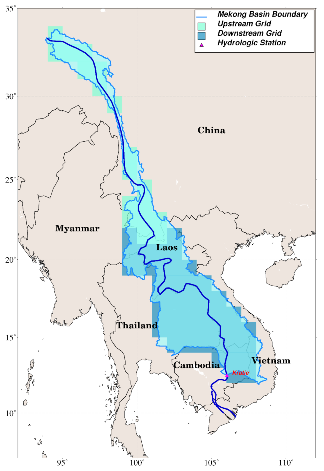
Figure 1. The Mekong Basin (bounded in light blue) and valid grids where the remotely sensed data was acquired in the upstream (light green) and downstream (dark blue) areas, along with the in situ hydrologic gauge (red triangle) station.
Remotesensing 13 00996 g001
Figure 2. Runoff time series of the Kratie station between 2003 and 2012.
Remotesensing 13 00996 g002
Figure 3. Spatial distribution of the Tropical Rainfall Measuring Mission precipitation (TRMM-P), the Moderate Resolution Imaging Spectroradiometer evapotranspiration (MODIS-ET), the Global Land Data Assimilation System Common Land Model evapotranspiration (GLDAS CLM-ET), and the Gravity Recovery and Climate Experiment terrestrial water storage (GRACE-S) with different data versions in August 2008.
Remotesensing 13 00996 g003
Figure 4. Flow diagram for determining the remotely sensed runoff estimates from the TRMM precipitation, the MODIS evapotranspiration, the GLDAS-CLM model-predicted evapotranspiration and terrestrial water storage, and the GRACE terrestrial water storage with different data versions.
Remotesensing 13 00996 g004
Figure 5. Estimated runoff of the entire Mekong Basin (MB) for Kratie station derived from the MODIS evapotranspiration data and several versions of the GRACE terrestrial water storage data.
Remotesensing 13 00996 g005
Figure 6. Estimated runoff of the entire MB for Kratie station derived from the GLDAS CLM evapotranspiration data and several versions of the GRACE terrestrial water storage data.
Remotesensing 13 00996 g006
Figure 7. Estimated runoff of the entire MB for Kratie station derived from the MODIS evapotranspiration data and several versions of the GLDAS terrestrial water storage data.
Remotesensing 13 00996 g007
Figure 8. Estimated runoff of the entire MB for Kratie station derived from the MODIS evapotranspiration and several versions of the GRACE terrestrial water storage with a three-month moving average.
Remotesensing 13 00996 g008
Figure 9. Taylor’s diagram showing the accuracy evaluation of the estimated runoff determined from the MODIS evapotranspiration data with several versions of GRACE terrestrial water storage data (triangle); the several versions of the GLDAS CLM evapotranspiration data with several versions of GRACE terrestrial water storage data (square); and the MODIS evapotranspiration data with several versions of GLDAS terrestrial water storage data (diamond), against in situ runoff (black dot) at Kratie station.
Remotesensing 13 00996 g009
Figure 10. Taylor’s diagram showing the accuracy evaluation of the estimated runoff after applying a three-month average for each data product determined from the MODIS evapotranspiration data with several versions of the GRACE terrestrial water storage data (triangle); the several versions of the GLDAS CLM evapotranspiration data with several versions of the GRACE terrestrial water storage data (square); and the MODIS evapotranspiration data with several versions of the GLDAS terrestrial water storage data (diamond), against in situ runoff (black dot) at Kratie station.
Remotesensing 13 00996 g010
Figure 11. The mean monthly remotely sensed runoff generated from the MODIS evapotranspiration data and several versions of the GRACE terrestrial water storages data after applying a three-month moving average and the in situ runoff at Kratie station.
Remotesensing 13 00996 g011
Figure 12. The mean monthly remotely sensed runoff generated from the GLDAS CLM evapotranspiration data and several versions of the GRACE terrestrial water storage data after applying a three-month moving average and the in situ runoff at Kratie station.
Remotesensing 13 00996 g012
Table 1. Remotely sensed data products and in situ gauge observations used in this study.
Hydrological ComponentData SourceSpatial ResolutionTemporal Resolution
PrecipitationTRMM 3B43 v7 0.25 ° × 0.25 ° 1 month
EvapotranspirationMOD16A2 0.5 ° × 0.5 ° 1 month
GLDAS CLM 1 ° × 1 ° 1 month
Terrestrial water storage changeGRACE 1 ° × 1 ° (mascon)/
3 ° × 3 ° (regular)
1 month
GLDAS (CLM, Mosaic, VIC, and the Noah model) 1 ° × 1 ° 1 month
RunoffGaugesPoint1 day
Table 2. Accuracy evaluation of the estimated monthly runoff generated from the MODIS-evapotranspiration and three versions of GRACE terrestrial water storage; GLDAS CLM-ET and three versions of GRACE terrestrial water storage; and MODIS-ET and several versions of GLDAS terrestrial water storage, using the same TRMM precipitation, against the in situ runoff at Kratie station.
Processing StrategyDataset CombinationsPCCRMSE
(mm/Month)
NSENRMSEMAPE
NoneMODIS + CSR RL050.86032.7980.5220.2021.055
MODIS + CSR RL060.84531.7630.5520.1960.927
MODIS + CSR Mascon0.83627.4650.6650.1690.644
CLM + CSR RL050.85135.9630.4260.2221.255
CLM + CSR RL060.81937.2420.3840.2301.445
CLM + CSR Mascon0.70741.8780.2210.2581.805
MODIS + CLM0.77061.371−0.6720.3782.136
MODIS + Mosaic0.75640.4640.2730.2491.263
MODIS + Noah0.85337.8830.3630.2341.258
MODIS + VIC0.80344.6890.1130.2751.578
Three-month averageMODIS + CSR RL050.90122.9660.7660.1420.816
MODIS + CSR RL060.89821.9520.7860.1350.715
MODIS + CSR Mascon0.93219.5800.8300.1210.377
CLM + CSR RL050.91831.1650.5690.1921.312
CLM + CSR RL060.91132.4120.5340.2001.476
CLM + CSR Mascon0.82838.0000.3590.2341.793
MODIS + CLM0.77151.175−0.1630.3151.934
MODIS + Mosaic0.78133.5360.5010.2071.137
MODIS + Noah0.87329.0460.6250.1791.070
MODIS + VIC0.81636.4830.4090.2251.376
Publisher’s Note: MDPI stays neutral with regard to jurisdictional claims in published maps and institutional affiliations.