Multiple Endmember Spectral Mixture Analysis (MESMA) Applied to the Study of Habitat Diversity in the Fine-Grained Landscapes of the Cantabrian Mountains

Abstract

Heterogeneous and patchy landscapes where vegetation and abiotic factors vary at small spatial scale (fine-grained landscapes) represent a challenge for habitat diversity mapping using remote sensing imagery. In this context, techniques of spectral mixture analysis may have an advantage over traditional methods of land cover classification because they allow to decompose the spectral signature of a mixed pixel into several endmembers and their respective abundances. In this work, we present the application of Multiple Endmember Spectral Mixture Analysis (MESMA) to quantify habitat diversity and assess the compositional turnover at different spatial scales in the fine-grained landscapes of the Cantabrian Mountains (northwestern Iberian Peninsula). A Landsat-8 OLI scene and high-resolution orthophotographs (25 cm) were used to build a region-specific spectral library of the main types of habitats in this region (arboreal vegetation; shrubby vegetation; herbaceous vegetation; rocks–soil and water bodies). We optimized the spectral library with the Iterative Endmember Selection (IES) method and we applied MESMA to unmix the Landsat scene into five fraction images representing the five defined habitats (root mean square error, RMSE ≤ 0.025 in 99.45% of the pixels). The fraction images were validated by linear regressions using 250 reference plots from the orthophotographs and then used to calculate habitat diversity at the pixel (α-diversity: 30 × 30 m), landscape (γ-diversity: 1 × 1 km) and regional (ε-diversity: 110 × 33 km) scales and the compositional turnover (β- and δ-diversity) according to Simpson’s diversity index. Richness and evenness were also computed. Results showed that fraction images were highly related to reference data (R² ≥ 0.73 and RMSE ≤ 0.18). In general, our findings indicated that habitat diversity was highly dependent on the spatial scale, with values for the Simpson index ranging from 0.20 ± 0.22 for α-diversity to 0.60 ± 0.09 for γ-diversity and 0.72 ± 0.11 for ε-diversity. Accordingly, we found β-diversity to be higher than δ-diversity. This work contributes to advance in the estimation of ecological diversity in complex landscapes, showing the potential of MESMA to quantify habitat diversity in a comprehensive way using Landsat imagery.

1. Introduction

A central point of natural sciences research is to identify, describe and understand biodiversity patterns for conservation purposes and natural resource management. The concept of biodiversity or biological diversity has changed rapidly during recent decades from a species diversity approach to a more comprehensible approach by also considering different hierarchical levels such as genes, populations, communities, ecosystems and landscapes, as well as their interactions [1,2]. Consequently, to evaluate all aspects of biological diversity is practically impossible, being necessary to focus on indicators that provide relevant, although relative, information [2]. Among them, habitats, which are defined as the type of site where an organism or population naturally occurs, are of high interest because they can be used as a proxy of diversity in different hierarchical levels. In this sense, the habitat heterogeneity hypothesis [3] states that increases in habitat diversity leads to increases in the variety of ways to exploit resources, thus increasing the complexity of ecosystems, species diversity [4,5] and, consequently, genetic diversity [6]. However, several studies suggest that the fulfillment of this hypothesis depends on the spatial scale of analysis and the target community [7,8].

It is generally assumed that biological diversity at any hierarchical level comprises two components: richness, which is defined as the number of different elements, and evenness, which indicates the equitability in the abundance distribution among different elements [2]. This concept has been integrated in several diversity indices based on the information theory that were originally proposed to measure the amount of disorder in a system. Among them, the Shannon [9] and Simpson [10] indices are the most widespread [11,12,13]. However, the Simpson index has a more intuitive interpretation, as it represents the probability that any two elements selected at random would be of different types, which unavoidably depends on richness and evenness [11].

Many authors have proposed a multiscale approach to analyze diversity because of its potential scale dependency [8,14,15], which has been demonstrated in several habitat diversity studies (e.g., [16,17]). In this sense, Whittaker [18] proposed the analysis of inventory diversity and compositional turnover (differentiation diversity) at different scales. Among the inventory diversity metrics, he defined (i) the α-diversity, or diversity at the plot level, with appropriate areas being between 100 m² and 1 ha for terrestrial plants [19]; (ii) the γ-diversity, or diversity at the landscape level, appropriate areas being of 1 km² or greater [19]; and (iii) the ε-diversity, or diversity at the regional scale. Among the compositional turnover metrics, Whittaker [18] defined the β-diversity as the difference in diversity between plot and landscape scales and the δ-diversity, or geographical differentiation, as the difference between the landscape and the regional scales.

Imagery from different satellites at relatively high and moderate spatial resolution, such as Landsat, Sentinel-2 and MODIS, has been commonly used to map habitat types [20,21,22] as well as habitat diversity at the landscape level [13,23,24]. In general, habitat mapping using remote sensing methods has been addressed with hard classifications, where each pixel is assigned to one unique type of habitat [25]. Among the most common are those classifications based on K-mean, ISODATA, maximum likelihood, decision trees, artificial neural networks or support vector machine algorithms [25]. However, hard classifications at the spatial resolution of Landsat, Sentinel or MODIS imagery (20 to 500 m) do not allow to obtain realistic spatial models in fragmented landscapes with predominance of small patches (i.e., fine-grained landscapes), where each image pixel can be a mixture of habitats or micro-habitats [25,26]. In this context, spectral unmixing, also known as spectral mixture analysis (SMA), is a key technique to address this challenge since it considers the spectrum of a single pixel as a weighted combination of constituent spectra (endmembers), the weight being the endmember fractions [27]. Thus, spectral unmixing provides fraction images allowing each pixel to have several and partial class memberships, which can be exploited in biodiversity studies by calculating diversity metrics even at the pixel level (α-diversity).

Multiple Endmember Spectral Mixture Analysis (MESMA) is an advanced method of linear SMA that calculates component fractions within a pixel [28]. As an improvement over basic linear SMA models, MESMA assumes that an image is composed of a large number of spectrally distinct endmembers, but individual pixels can be composed of a limited subset of these components [27,28]. Accordingly, MESMA allows a large number of endmembers to be used across a scene, but each pixel is analyzed and modeled independently with different numbers and types of endmembers [28,29,30], avoiding the overfitting caused by the use of many endmembers and, also, the large residuals that would cause the lack of specific endmembers in the analysis [31]. Previous research has focused on applying MESMA to map natural [28,29,32,33,34,35] and anthropized [31,36,37,38,39] landscapes, with the accuracy of MESMA fraction images largely varying depending on the land cover class [37,39]. In general, these studies have shown the capacity of MESMA to generate a number of land cover fraction images ranging from three [28,29,33,34] to five [31,32,39], which could be applied to the analysis of habitat diversity. However, to date, we have not found studies exploring the potentiality of MESMA for ecological applications such as biodiversity assessments.

Given the current challenges in habitat diversity monitoring and the potential benefits of spectral unmixing techniques, our study aims to use, for the first time, MESMA to accomplish a comprehensive analysis of habitat diversity in fine-grained landscapes, using the Cantabrian Mountains (northwest Iberian Peninsula) as a study case. Specifically, we aim (i) to analyze the potentiality of MESMA to model the fractional cover of the main types of habitat and (ii) to characterize habitat diversity at different scales, from the pixel level to the regional scale (α-, γ- and ε-diversity), as well as the compositional turnover (β- and δ-diversity).

2. Materials and Methods

The methodology followed in this study is structured in five blocks (Figure 1): (i) selection of the study site, (ii) data sources and preparatory steps, (iii) MESMA procedure, (iv) accuracy assessment of MESMA fraction images and (v) habitat diversity analysis.

2.1. Study Site

The study site is a framework of 110 × 33 km sited in the Cantabrian Mountains (Figure 2a,b), which are located in the northwest of the Iberian Peninsula, between the Eurosiberian and Mediterranean biogeographical regions. They exhibit a high elevation gradient (from sea level up to 2650 m), a mean annual precipitation from 700 to 2200 mm and a mean annual temperature from 4 to 14 °C [40] in a distance of less than 30 km, causing a high biodiversity and the existence of several endemic species [41]. The main vegetation types in the valleys are cultivated and grazed meadows and riparian forests. In the uplands, there are beech (Fagus sylvatica L.), oak (Quercus pyrenaica Willd., Q. petraea (Matt.), Liebl., Q. robur L. and Q. ilex L.) and birch (Betula spp.) deciduous forests, pine plantations (Pinus sylvestris L, P. nigra Arn. and P. radiata D. Don) as well as heathlands and shrublands dominated by Ericaceae, Fabaceae and Cistaceae plant species. Forests and shrublands are often interspersed with pastures and grasslands. The tops of the mountains are usually dominated by rocks, scree and natural grasslands, with variable cover of shrublands.

The Cantabrian Mountains were considered appropriate for this study for several reasons: (i) their landscapes (which include mountain massifs, intra-montane valleys and bocage landscapes) show a high complexity as they consist of fine-grained mosaics of natural and semi-natural habitats [42,43]. This fact encourages the use of unmixing methods for habitat mapping when using satellite multispectral imagery of coarser grain size than landscape (see Figure 2c–e to visually understand the inconvenience of assigning a 30-m pixel to a single habitat class). (ii) This region sustains a high diversity of species and ecosystems [44] and has many habitats that are considered as a conservation priority by the European Union (Council Directive 92/43/EEC) [45], which motivates the advancement of habitat mapping and monitoring methods relevant for conservation actions. (iii) The Cantabrian Mountains can be considered as a natural field laboratory to study habitat diversity and its relationships with rural abandonment and land use change, as they have experienced an intense change during recent decades [46,47].

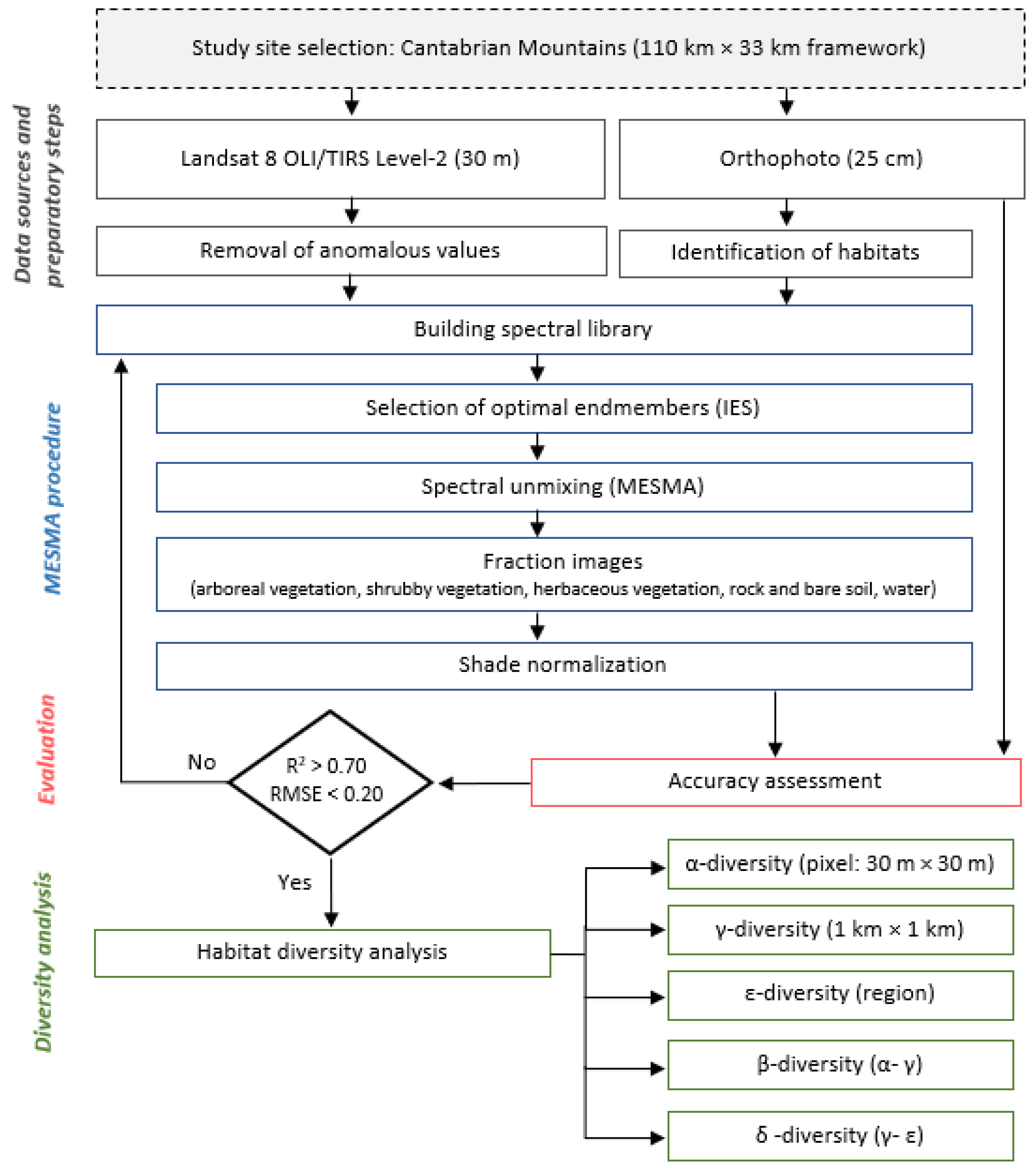
2.2. Data Sources and Preparatory Steps

2.2.1. Landsat Imagery

A cloud-free Landsat-8 OLI scene for the study area (Landsat path 203/row 30) from 11 August 2017, was selected and downloaded from the U.S. Geological Survey (USGS) server [48]. Specifically, we used a Landsat collection 1 Level-2 scene (LC082030302017081101T1-SC20200826092241), which is radiometrically and geometrically corrected, georeferenced to a Universal Transversal Mercator (UTM) projection and corrected for atmospheric effects with the Land Surface Reflectance Code (LaSRC) [49]. Thus, this product contains the following subset of Landsat reflective bands in land surface reflectance:

• Band 1: ultra-blue, 0.43–0.45-µm wavelength
• Band 2: blue, 0.45–0.51-µm wavelength
• Band 3: green, 0.53–0.59-µm wavelength
• Band 4: red, 0.64–0.67-µm wavelength
• Band 5: near-infrared, 0.85–0.88-µm wavelength
• Band 6: shortwave infrared 1, 1.57–1.65-µm wavelength
• Band 7: shortwave infrared 2, 2.11–2.29-µm wavelength

Landsat-8 OLI collection 1 Level-2 surface reflectance scenes are provided by the USGS systematically scaled to 10,000. However, anomalous values (≤0 or ≥10,000) are usual. In view of this issue, we removed all values ≤0 and ≥10,000 from the Landsat scene, resulting in reflectance values between 1 and 9999.

2.2.2. Reference Data

In this study, we used orthophotographs at very high spatial resolution (25 cm) as reference data to identify the main types of habitat, delineate pure habitats and assess the accuracy of Landsat-8-derived products. Specifically, we used the digital orthophotographs taken by the Spanish National Center of Geographic Information in July 2017, through the Spanish National Program for Aerial Orthophoto [50]. This is the latest series currently available (1 December 2020) and the flight date coincides with that of the Landsat-8 image used in this study.

Five types of habitat were differentiated for this study (arboreal vegetation; shrubby vegetation; herbaceous vegetation; rocks and bare soil and water bodies) according to previous work in the Cantabrian Mountains [41] and to a visual inspection of the orthophotographs at a scale of 1:1000.

For accuracy assessment purposes, we established 250 plots of 30 × 30 m spatially coincident with Landsat pixels. We followed a stratified random design, assigning a set of 50 plots to each habitat type in the orthophotographs (Figure 2b). Then, we used the orthophotos, to quantify the percentage cover correspondent to each habitat type in each plot. To improve the efficiency and accuracy of this process, plots were divided into 100 square cells of 3 × 3 m using the Polygon Divider plugin [51] in the QGIS 3.14 geographic information system software [52]. Then, each cell was visually classified into a unique habitat type and the proportion of cells corresponding to each class was calculated. In this way, we assigned information of the fractional cover of all types of habitat in each 30 × 30-m reference plot.

2.3. MESMA Procedure

2.3.1. Spectral Library: Candidate and Optimal Endmembers

The first step to perform MESMA was to build a spectral library with candidate endmembers for each of the five classes contemplated to unmix the Landsat-8 scene (arboreal vegetation; shrubby vegetation; herbaceous vegetation; rocks and bare soil and water bodies). Candidate endmember spectra can be obtained from spectral libraries (reference endmembers), which are built using field and laboratory measurements or radiative transfer models, or from the scenes used in the study (image endmembers) [27]. In this work, we have used the last approach, because image endmembers have the advantages of (i) being easily obtained; (ii) they can be collected at the same scale as the image data, capturing the multiple scattering environment of canopies [36]; and (iii) spectra are influenced by the same imagery corrections as the scene used in the study [53].

Image endmembers for each habitat type were extracted from the pre-processed Landsat-8 surface reflectance scene using 250 polygons, meeting the following criteria: (i) polygon size was fixed to 60 × 60 m to ensure that four Landsat-8 pixels fall within each polygon; (ii) the polygon and the surrounding area (30-m buffer) were dominated by a single habitat type (>75%), according to the orthophoto; (iii) plots were distanced at least 60 m from validation plots to ensure independence between endmember data and validation data; and (iv) polygons were distributed with equitability among the different types of habitat (50 plots per habitat, with 200 pixels per habitat and a total of 1000 pixels). Accordingly, we extracted 1000 candidate image endmembers (200 endmembers for each habitat type) using the Create Library tool from the Spectral Library plugin [54], which is implemented in QGIS [52].

Once the candidate endmembers are selected, it is critical to optimize the spectral library by defining a high-quality set of image endmembers. This process contributes to reduce the computational costs and to increase the accuracy of MESMA [31,53,55]. There are several techniques for pruning spectral libraries according to the relative value of each individual endmember. In this study, we used Iterative Endmember Selection (IES) [32], which is an automated method that finds the set of endmembers that produce the highest Cohen’s kappa value by iteratively adding or removing endmembers. Firstly, the algorithm compares all possible pairs of endmembers, retaining the two endmembers that reach the highest kappa value for classifying all the spectral library using MESMA. Then, the algorithm automatically checks the ability of additional endmembers to increase kappa, and the process is repeated until the kappa value does not increase any more. Thus, IES not only considers within-class variability, as many endmember selection methods do [55], but also confusion between classes. For the IES procedure, we set the minimum and maximum allowable endmember fractional constrains to 0.00 and 1.00, respectively, and the root mean square error (RMSE) value was constrained to 0.025. The spectral library processed in this way is referred as IES library for the remainder of this document. The spectral library was optimized using the IES tool from the Spectral Library plugin [54], which is implemented in QGIS [52] and based on VIPER Tools 2.0 developed by the VIPER Lab at UC Santa Barbara.

2.3.2. Spectral Unmixing: Obtention of Fraction Images and Shade Normalization

The IES library was used to map the fractional abundance of each habitat type in each pixel of the Landsat-8 scene using MESMA. In view of the composition and the fine-grain landscape of the study site (Figure 2), we assumed that every pixel in the Landsat-8 scene can be modeled by a linear combination of one to five types of habitat and a shade fraction that is typically present in all pixels. Accordingly, MESMA was applied, analyzing all the potential combinations for each pixel; i.e., two-endmember models (one habitat type + shade), three-endmember models (two types of habitat + shade), four-endmember models (three types of habitat + shade), five-endmember models (four types of habitat + shade) and six-endmember models (five types of habitat + shade). The shade endmember was defined as photometric shade, setting reflectance values to zero. We set the minimum and maximum allowable endmember fractional values to 0.00 and 1.00, respectively, because values outside this range cannot be achieved in the field. We constrained the maximum allowable shade fraction to 0.80 according to [36,56,57] recommendations. The performance of all endmember models that meet all the above criteria was evaluated by the RMSE and the model with the lowest RMSE was selected for each pixel and recorded. Hence, we generated three output products: (i) an image with the models given in the form of the endmember number of the spectral library, (ii) an RMSE image and (iii) the fraction images of each habitat type and shade. Finally, the output fraction images were shade normalized to obtain the relative abundance of non-shade endmembers (types of habitat) for each pixel. MESMAs and shade normalization were carried out with the MESMA and Shade normalization tools, respectively, from the MESMA plugin [58], which is implemented in QGIS [52] and based on VIPER Tools 2.0 developed by the VIPER Lab at UC Santa Barbara.

2.4. Accuracy Assessment of MESMA Fraction Images

We used 250 reference plots (see Section 2.2.2) with values of the fractional cover of each habitat type to assess the performance of the sub-pixel fraction estimates from MESMA. Specifically, using the reference plot centroids, we sampled the raster values (fractional covers) using the Point Sampling Tool [59] in QGIS [52], and then, we used them to perform bivariate linear regressions between each shade-normalized MESMA fraction (predictor variable) and the reference data (response variable), from which we calculated the significance of the correlations (P), the coefficient of determination (R²) and the RMSE. Linear regressions were performed using R software [60].

2.5. Diversity Analysis

After ensuring the accuracy of all shade-normalized MESMA fraction images (minimum requirements of R² > 0.70 and RMSE < 0.20), they were used to map habitat richness, evenness and diversity at different spatial scales (α-diversity: 30 × 30 m, γ-diversity: 1 × 1 km, ε-diversity: 110 × 33 km) as well as to calculate the mean values and standard deviations for the entire study area.

Habitat richness was calculated as the number of different types of habitat. According to the number of habitat types considered in this work, the maximum allowable richness is 5.

Habitat evenness was calculated using Simpson’s Evenness Index (Equation (1)) [10,12]. This index is unitless and approaches 0 as the distribution of area among the different habitat types becomes increasingly uneven, whereas it approaches 1 when proportional abundances are the same.

$$E=\frac{1-{{\displaystyle \sum }}_{i=1}^m{P}_i^2}{1-\left(\frac{1}{m}\right)}$$

(1)

where E is Simpson’s Evenness Index; P_i is the proportion occupied by habitat type (class) i at the working scale and m is the number of habitat types present at the working scale.

Habitat diversity was calculated using Simpson’s Diversity Index (Equation (2)) [10]. This index approaches 0 when there is a low richness and the distribution among the different habitat types becomes increasingly uneven, and it approaches 1 when there is a high richness and the proportional abundances are the same. The maximum allowable value for this index in this study, where the maximum richness is 5, is 0.80.

$$D=1-{\displaystyle \sum }_{i=1}^m{P}_i^2$$

(2)

where D is Simpson’s Diversity Index; P_i is the proportion occupied by habitat type (class) i at the working scale and m is the number of habitat types present at the working scale.

Geo-processing to obtain richness, evenness (E) and diversity (D) products at 30 × 30 m was carried out by applying the corresponding functions (richness, Equations (1) and (2)) to the fraction images from MESMA in the Raster Calculator tool in QGIS [52]. To obtain the richness, E and D at 1 × 1 km and 110 × 33 km, we computed all fraction images at these spatial resolutions by averaging the values from the original fraction images (30 × 30-m spatial resolution) in each 1 × 1-km cell and in the entire study area (110 × 33 km), respectively. This process was accomplished using the Zonal Statistics tool over a 1 × 1-km grid and 110 × 33-km polygon, respectively, in QGIS [52].

Moreover, we used Simpson’s Diversity Index at different scales to calculate the β-diversity (turnover between γ- and α-diversity) (Equation (3)) and δ-diversity (turnover between ε- and γ-diversity) (Equation (4)).

$$\mathsf{\beta }\mathrm{diversity}=D\gamma - D\alpha$$

(3)

$$\mathsf{\delta }\mathrm{diversity}=D\epsilon -D\gamma$$

(4)

where D$\alpha$ is Simpson’s Diversity Index calculated at the pixel level (30 × 30 m), Dγ is Simpson’s Diversity Index calculated at 1 × 1 km and Dε is the Simpson Diversity Index for the entire study region (110 × 33 km). Geo-processing to obtain β- and δ-diversity products was carried out by implementing Equation (3) and Equation (4) in the Raster Calculator tool in QGIS [52].

3. Results

3.1. MESMA Results and Accuracy Assessment

3.1.1. Optimal Endmembers

In the IES procedure applied to obtain a set of optimal endmembers (IES library), kappa values increased from 0.17 when using one candidate endmember to 0.78 when using five candidate endmembers (one endmember from each habitat type). The maximum within-library kappa peaked at 0.95, using 31 endmembers. Thus, the final IES library consisted of 31 endmembers (Figure 3), which were unequally distributed among habitat classes: arboreal vegetation—four spectra; shrubby vegetation—10 spectra; herbaceous vegetation—seven spectra; rock and bare soil—nine spectra; water—one spectrum. The maximum reflectance of arboreal and shrubby vegetation endmembers was detected in the near-infrared region (B5), and for herbaceous vegetation, in both the near-infrared and shortwave-infrared regions (B5 and B6). The spectral signatures of rock and bare soil endmembers differed because they showed higher reflectance values than vegetation endmembers for the ultra-blue, blue, green and red (B1 to B4) and the highest reflectance in the shortwave-infrared region (B6). On the contrary, the water spectrum showed low reflectance values for all bands, with the reflectance in the green region (B3) being the highest.

3.1.2. Spectral Unmixing

The comparison of all potential combinations of the spectra included in the IES library in all possible class models with MESMA signified the analysis of the performance of 8799 models in each Landsat pixel. Specifically, 31 one-endmember models (one habitat type + shade), 357 three-endmember models (two habitat types + shade), 1849 four-endmember models (three habitat types + shade), 4042 five-endmember models (four habitat types + shade) and 2520 six-endmember models (five habitat types + shade) were analyzed for each pixel.

MESMA modeled 99.45% of the pixels with an RMSE ≤ 0.025, whereas 99.61% of pixels were modeled with an RMSE ≤ 0.05. Moreover, the MESMA results after shade-normalization demonstrated that almost one half of the pixels in the study area were successfully modeled as a mixture of two habitats (

Table 1. Number and relative abundance of pixels of the study area with the presence of each habitat type, and class models for each level of complexity (one-, two- and three-endmember models). The table also shows the cover in percentage (mean ± standard deviation of each habitat type in the study area). Results were calculated from the MESMA fraction images after shade normalization. See Table A1 for further information.

	Pixels (n)	Pixels (%)	Cover (Mean ± SD)
Classes
Arboreal vegetation	1,639,730	39.98	23.96 ± 33.59
Shrubby vegetation	1,792,223	43.70	31.49 ± 39.86
Herbaceous vegetation	1,767,967	43.11	33.93 ± 42.50
Rock and bare soil	856,272	20.88	10.05 ± 24.51
Water	22,736	0.55	0.53 ± 7.16
Class models
One-habitat type model	2,123,946	51.79
Two-habitat type model	1,975,994	48.18
Three-habitat type model	998	0.02
Total	4,100,938	100

). Specifically, 51.79% of pixels were modeled using a single endmember from one habitat type, whereas 48.18% of pixels were modeled by endmembers from two types of habitat, the most frequent mixtures being arboreal and shrubby vegetation and arboreal and herbaceous vegetation (

Table A1. Number and relative abundance of pixels of the study for each combination of habitat types. Results were calculated from the MESMA fraction images after shade normalization.

	Pixels (n)	Pixels (%)
Class models
Arboreal vegetation	293,772	7.16
Shrubby vegetation	725,083	17.68
Herbaceous vegetation	892,727	21.77
Rock (and bare soil)	191,955	4.68
Water	20,409	0.50
Arboreal and herbaceous	438,983	10.70
Arboreal, herbaceous and rock	867	0.02
Arboreal, herbaceous and water	1	0.00
Arboreal and rock	136,413	3.33
Arboreal, rock and water	99	0.00
Arboreal and shrubby	769,141	18.76
Arboreal and water	454	0.01
Herbaceous and rock	331,387	8.08
Herbaceous, rock and shrubby	21	0.00
Herbaceous, rock and water	10	0.00
Herbaceous and shrubby	103,727	2.53
Herbaceous and water	244	0.01
Rock and shrubby	194,126	4.73
Rock and water	1394	0.03
Shrubby and water	125	0.00
Total	4,100,938	100

). Only 0.02% of pixels required the use of endmembers from three types of habitat to be modeled with the lowest RMSE, and they correspond mainly to the mixture of arboreal vegetation, herbaceous vegetation and rock–bare soil (Table A1).

Focusing on the types of habitats, MESMA modeled arboreal vegetation fractions in 39.40% of pixels, shrubby and herbaceous vegetation fractions in approximately 43% of pixels and rock and bare soil classes in 20.88% of pixels. Water fractions were present in 0.55% of pixels. Moreover, shade-normalized MESMA fraction images allowed to calculate the mean cover of each habitat type (Table 1). In this sense, we found that the study area was dominated by herbaceous, shrubby and arboreal vegetation (33.93%, 31.49% and 23.96%, respectively), whereas rocks and bare soil (10.05%) and water bodies (0.53%) were less abundant.

3.1.3. Accuracy Assessment of MESMA Fraction Images

The relationships between reference and modeled fractions of the five types of habitat were statistically significant in all cases (p < 0.001). Besides, MESMA fraction images showed R² values ≥ 0.73 and RMSE ≤ 0.18 when predicting the fractional cover of the five types of habitat (Figure 4). Analyzing each habitat type, the highest predictive accuracy was for water bodies (R² = 0.99; RMSE = 0.04). Rocks and bare soil also were modeled with a high accuracy (R² = 0.90; RMSE = 0.11). Linear relationships with herbaceous vegetation showed R² = 0.78 and RMSE = 0.15; relationships with shrubby and arboreal vegetation cover showed R² = 0.73 and RMSE of 0.17 and 0.18, respectively.

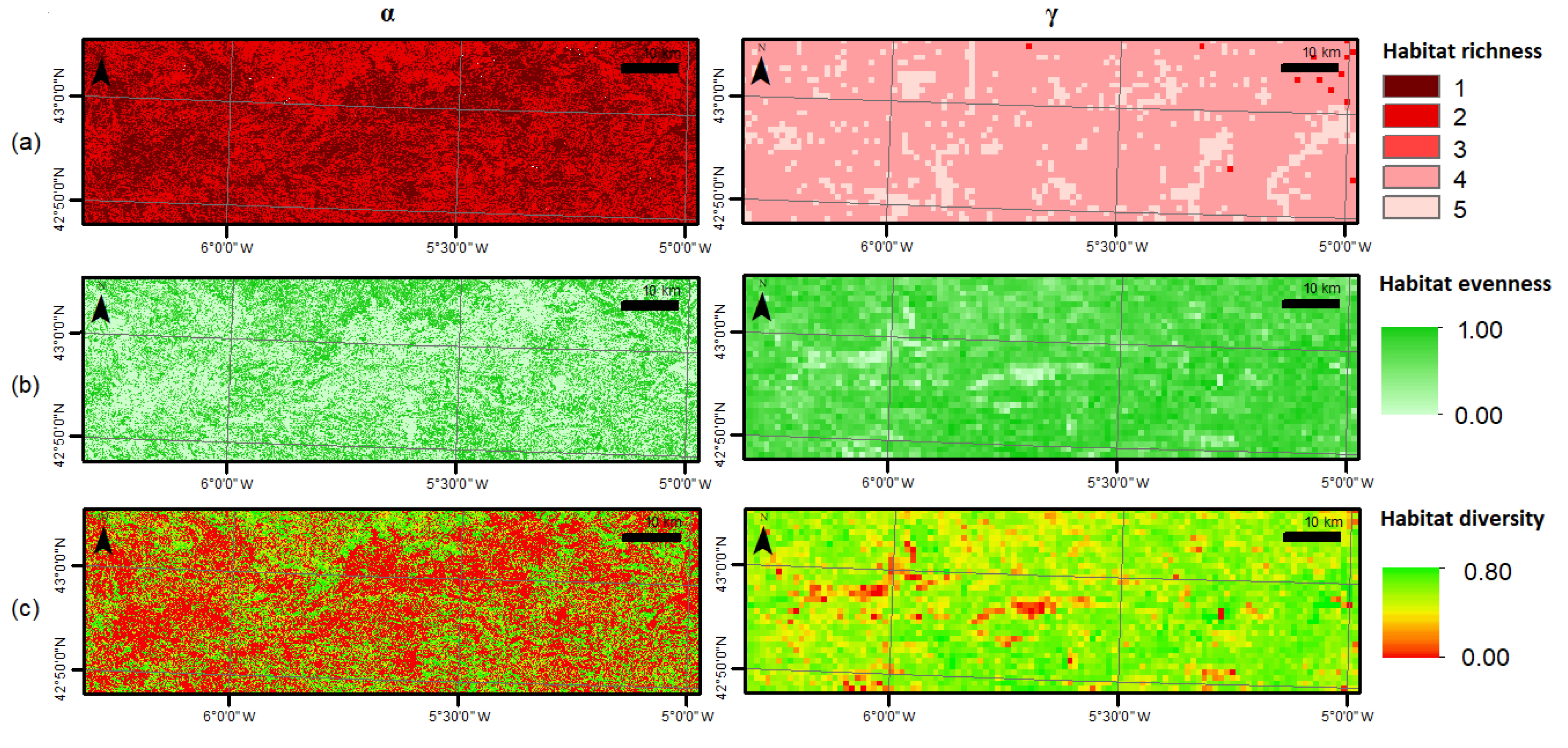
3.2. Habitat Diversity

Values of habitat richness, evenness and diversity in the Cantabrian Mountains were scale-dependent (

Table 2. Mean values of α-, γ- and ε-diversity metrics (habitat richness, habitat evenness and habitat diversity), as well as β- and δ-diversity values in the study site.

Diversity Metric	Spatial Scale (km2)	Value (Mean ± SD)
α-richness	0.0009	1.48 ± 0.50
γ-richness	1	4.15 ± 0.36
ε-richness	3630	5.00 ± 0.00
α-evenness *	0.0009	0.40 ± 0.43 *
γ-evenness	1	0.80 ± 0.12
ε-evenness	3630	0.90 ± 0.00
α-diversity	0.0009	0.20 ± 0.22
γ-diversity	1	0.60 ± 0.09
ε-diversity	3630	0.72 ± 0.00
β-diversity	0.0009	0.40 ± 0.23
δ-diversity	1	0.11 ± 0.09

* The area with α-richness = 1 (indeterminate form in evenness according to Equation (2)) was fixed to 0.

). Habitat richness increased from the pixel level at 30 × 30 m (mean α-richness = 1.48) to the landscape scale at 1 × 1 km (mean γ-richness = 4.15), with the maximum value being found at regional scale (ε-richness = 5). Similarly, habitat evenness, measured as the Simpson Evenness Index, increased from the pixel level (mean α-evenness = 0.40) to the landscape spatial scale (γ-evenness = 0.80), with the maximum equitability among habitat classes being found at the regional scale (ε-evenness = 0.90). The mean values of the Simpson Diversity Index also increased with the sampled area, particularly from the pixel (α-diversity = 0.20) to the landscape scale (γ-diversity = 0.60). The habitat diversity at the regional scale (ε-diversity) was 0.72.

In relation to the compositional turnover, the largest differences in habitat diversity were found when upscaling from the pixel to the landscape scale (β-diversity = 0.40). Habitat diversity slightly changed at resolutions coarser than 1 × 1 km (δ-diversity = 0.11).

Figure 5 shows the spatial patterns of habitat richness, evenness and diversity in the study area. At the pixel level, α-richness varied between one or two in most of the study area (Figure 5a), with the highest values spatially matching to forests, which are often combined with other types of habitat (See Figure A1 in the Appendix A). On the contrary, at landscape scale, four and five types of habitat predominated (Figure 5a), with the highest γ-richness in areas occupied by water bodies (reservoirs, lakes and rivers), which are scarcer and less spatially connected than the rest of habitats (Figure A1). In relation to habitat evenness (Figure 5b), it was directly related to habitat richness at the pixel level, whereas at landscape scale, we found the lowest evenness values in lowlands dominated by grasslands and meadows (Figure A1). Habitat diversity (Figure 5c) showed spatial heterogeneity at both pixel and landscape levels. In this sense, the spatial patterns of α-diversity were coincident with those of α-richness and evenness, whereas the spatial patterns γ-diversity were more related to γ-evenness than to γ-richness.

The spatial patterns of the compositional turnover (Figure 6) indicate that the diversity, in most of the study area, increased when upscaling from the pixel to the landscape level (97.88% of the study area showed a β-diversity > 0) as well as from the landscape to the regional level (96.00% of the study area showed a δ-diversity > 0). However, increases were much larger at fine spatial resolutions, with δ-diversity values being close to 0 in most of the study area.

4. Discussion

Our results showed the capacity of MESMA to model the main types of habitat present in the study region (arboreal vegetation, shrubby vegetation, herbaceous vegetation, rocks and bare soil and water bodies) as well as the suitability of fraction images obtained from MESMA to perform a thorough analysis of habitat diversity and compositional turnover in the fine-grained landscapes of the Cantabrian Mountains.

Although many studies have applied MESMA to differentiate photosynthetic vegetation, non-photosynthetic vegetation and soil [36,61], and impervious elements [57], and to map the fractional abundance of vegetation types [32] and even the fractional cover of bio-physical variables in disturbed areas [31,53], this is the first work in which MESMA is applied to analyze habitat diversity. The appropriateness and potentiality of MESMA for determining habitat fractions and habitat diversity in fine-grained landscapes, such as those of the Cantabrian Mountains, can be justified by the three following reasons supported by our findings. (i) Firstly, the need of 31 endmembers to build an optimized image-specific spectral library reflects that the use of multiple endmembers is needed for accurate mapping. This indicates that this challenge would not have been accurately addressed by simple SMA, where the maximum number of endmembers would be constrained to the number of habitat types plus shade [27,53]. Moreover, in relation to this issue, we underline the relevance of an appropriate selection of endmembers, which must be linearly independent, representative of the spectra and spatially generalizable [29], and we point out that the classification accuracy reached in our optimized spectral library (kappa = 0.95) using the iterative endmember selection method was better than that reported in the reviewed literature [32,37,62,63]. (ii) Secondly, the MESMA results revealed that the spectra of almost the half of the 30 × 30-m pixels in the study area were modeled using two endmembers from different type of habitats, whereas the other half were modeled using a single endmember. The need of multiple endmembers to accurately model spectra has been found in other studies [28,36,61,64] when characterizing dominant surface types and indicates that habitat mapping as well as habitat diversity analysis in fine-grained landscapes should be addressed either by spectral unmixing methods such as MESMA or using imagery at a higher spatial resolution, such as UAV-derived imagery or satellite imagery at very high spatial resolution. (iii) Lastly, we found that the subpixel abundance estimates obtained from MESMA were highly accurate—results showing very low errors (RMSE values between 0.04 and 0.18) and high coefficients of determination (R² between 0.73 and 0.99) for the fractions of the five target habitats. These results are in concordance with those obtained in previous studies that used multispectral and hyperspectral data to quantify the fractional cover of soil and vegetation types in other regions with different fine-grained landscape patterns [65,66,67,68], such as orchards [67,69], cultivated lands and urban areas, where impervious surfaces are interspersed with gardens and other habitat types [36,37,65,66]. This suggests the potential appropriateness of MESMA for habitat mapping and, consequently, habitat diversity analysis in other regions, although this fact should be confirmed by further research.

Hence, our results show the use of MESMA to characterize habitat diversity and compositional turnover in the fine-grained landscapes of the Cantabrian Mountains. The analysis at the different scales proposed by Whittaker [18] revealed a high scale-dependency of habitat diversity, with increases being particularly intense from the pixel (Simpson’s Diversity Index = 0.20) to the landscape (Simpson’s Diversity Index = 0.60) level. Values of habitat diversity at the regional scale were even higher (Simpson’s Diversity Index increased = 0.72) but close to those obtained at the landscape scale. Accordingly, β-diversity was higher than δ-diversity. The scale-dependency of habitat diversity has been previously reported [14,15,16,17] and confirms the appropriateness of a multi-scale analysis in this type of landscape. Moreover, our results indicated that the spatial patterns of habitat diversity were parallel to the spatial patterns of richness at the pixel level (α-diversity), whereas they were more similar to the spatial patterns of evenness at the landscape (γ-diversity) and regional (ε-diversity) levels because, in general, most habitat types were present when working at scales above 1 km². These results indicate that landscapes and regions sustain a higher biodiversity and should be considered by land managers and policy makers to spatially define priority areas for conservation purposes.

Our work provides a useful basis for habitat diversity mapping in fine-grained landscapes when using moderate spatial resolution imagery. It opens the possibility of conducting habitat diversity assessments across time, taking advantage of the availability of Landsat scenes since the 1970s [70] and the possibility of building multi-temporal libraries [71]. Likewise, this study presents a suitable method to address habitat diversity analysis in those landscapes where two types of habitat coexist at the pixel level, and we encourage validation of this methodology in other landscapes and regions across the globe, particularly in areas where more than two component mixtures are common. Future research to make advancements in the remote sensing discipline can address the potentiality of non-linear spectral unmixing methods for habitat diversity mapping in complex regions, as this method can account for both the effects of multiple scattering and endmember variability [27] and, therefore, contributes to improve the accuracy of fraction images [72,73]. Moreover, higher spectral resolution imagery can also contribute to increase the spectral separability among endmembers, which is essential for accurate unmixing in both linear and non-linear approaches [73].

5. Conclusions

Habitat diversity mapping in fine-grained territories is an important challenge that can be resolved either by using imagery of high spatial resolution or applying spectral unmixing methods to moderate spatial resolution imagery, such as Landsat scenes.

Multiple Endmember Spectral Mixture Analysis (MESMA) is useful for quantifying the fractional cover of the main habitat types present in the Cantabrian Mountains in a per-pixel basis. Thereafter, fractional cover images can be used to calculate habitat diversity at the pixel, landscape and regional levels (α-, γ- and ε-diversity) and are suitable for analyzing the compositional turnover (β- and δ-diversity).

Habitat diversity in the Cantabrian Mountains is scale-dependent, and therefore, diversity analysis should be performed at different spatial scales. Habitat diversity strongly increased with area from the pixel (α-diversity) to the landscape level (γ-diversity), with β-diversity being higher than δ-diversity. Moreover, we found that the spatial patterns of diversity were closely related to the spatial patterns of evenness at the landscape level.

References

1. Poiani, K.A.; Richter, B.D.; Anderson, M.G.; Richter, H.E. Biodiversity Conservation at Multiple Scales: Functional Sites, Landscapes, and Networks. BioScience 2000, 50, 133–146. [Google Scholar] [CrossRef] [Green Version]
2. Léveque, C.; Mounlou, J.-C. Biodiversity; Wiley: Cornwall, UK, 2003; pp. 13–38. [Google Scholar]
3. MacArthur, R.H.; MacArthur, J.W. On bird species diversity. Ecology 1961, 42, 594–598. [Google Scholar] [CrossRef]
4. Tews, J.; Brose, U.; Grimm, V.; Tielborger, K.; Wichmann, M.C.; Schwager, M.; Jeltsch, F. Animal species diversity driven by habitat heterogeneity/diversity: The importance of keystone structures. J. Biogeogr. 2004, 31, 79–92. [Google Scholar] [CrossRef] [Green Version]
5. Pacheco, R.; Vasconcelos, H.L. Habitat diversity enhances ant diversity in a naturally heterogeneous Brazilian landscape. Biodivers. Conserv. 2012, 21, 797–809. [Google Scholar] [CrossRef]
6. Currat, M.; Ray, N.; Excoffier, L. SPLATCHE: A program to simulate genetic diversity taking into account environmental heterogeneity. Mol. Ecol. Notes 2004, 4, 139–142. [Google Scholar] [CrossRef] [Green Version]
7. Vanbergen, A.J.; Watt, A.D.; Mitchell, R.; Truscott, A.-M.; Palmer, S.C.F.; Ivits, E.; Eggleton, P.; Jones, T.H.; Sousa, J.P. Scale-specific correlations between habitat heterogeneity and soil fauna diversity along a landscape structure gradient. Oecologia 2007, 153, 713–725. [Google Scholar] [CrossRef]
8. García-Llamas, P.; Calvo, L.; De la Cruz, M.; Suárez-Seoane, S. Landscape heterogeneity as a surrogate of biodiversity in mountain systems: What is the most appropriate spatial analytical unit? Ecol. Indic. 2018, 85, 285–294. [Google Scholar] [CrossRef]
9. Shannon, C.E.; Weaver, W. The Mathematical Theory of Communication; University of Illinois Press: Urbana, IL, USA, 1949. [Google Scholar]
10. Simpson, E.H. Measurement of diversity. Nature 1949, 163, 688. [Google Scholar] [CrossRef]
11. Margalef, D.R. Information theory in ecology. Gen. Syst. 1958, 3, 36–71. [Google Scholar]
12. Smith, B.; Wilson, J.B. A Consumer’s Guide to Evenness Indices. Oikos 1996, 76, 70–82. [Google Scholar] [CrossRef]
13. Rocchini, D.; Delucchi, L.; Bacaro, G.; Cavallini, P.; Feilhauer, H.; Foody, G.M.; He, K.S.; Nagendra, H.; Porta, C.; Ricotta, C.; et al. Calculating landscape diversity with information-theory based indices: A GRASS GIS solution. Ecol. Inf. 2013, 17, 82–93. [Google Scholar] [CrossRef]
14. Whittaker, R.J.; Willis, K.J.; Field, R. Scale and species richness: Towards a general, hierarchical theory of species diversity. J. Biogeogr. 2001, 28, 453–470. [Google Scholar] [CrossRef] [Green Version]
15. McGarigal, K.; Wan, H.Y.; Zeller, K.A.; Timm, B.C.; Cushman, S.A. Multi-scale habitat selection modeling: A review and outlook. Landsc. Ecol. 2016, 31, 1161–1175. [Google Scholar] [CrossRef]
16. Fox, B.J.; Fox, M.D. Factors determining mammal species richness on habitat islands and isolates: Habitat diversity, disturbance, species interactions and guild assembly rules. Glob. Ecol. Biogeogr. 2000, 9, 19–37. [Google Scholar] [CrossRef]
17. Kallimanis, A.S.; Mazaris, A.D.; Tzanopoulos, J.; Halley, J.M.; Pantis, J.D.; Sgardelis, S.P. How does habitat diversity affect the species–area relationship? Glob. Ecol. Biogeogr. 2008, 17, 532–538. [Google Scholar] [CrossRef]
18. Whittaker, R.H. Vegetation of the Siskiyou Mountains, Oregon and California. Ecol. Monogr. 1960, 30, 279–338. [Google Scholar] [CrossRef]
19. Shmida, A.; Wilson, M.V. Biological determinants of species diversity. J. Biogeogr. 1985, 12, 1–20. [Google Scholar] [CrossRef]
20. Weber, D.; Schaepman-Strub, G.; Ecker, K. Predicting habitat quality of protected dry grasslands using Landsat NDVI phenology. Ecol. Indic. 2018, 91, 447–460. [Google Scholar] [CrossRef]
21. Erinjery, J.; Singh, M.; Kent, R. Mapping and assessment of vegetation types in the tropical rainforests of the Western Ghats using multispectral Sentinel-2 and SAR Sentinel-1 satellite imagery. Remote Sens. Environ. 2018, 216, 345–354. [Google Scholar] [CrossRef]
22. Clerici, N.; Weissteiner, C.J.; Gerard, F. Exploring the Use of MODIS NDVI-Based Phenology Indicators for Classifying Forest General Habitat Categories. Remote Sens. 2012, 4, 1781–1803. [Google Scholar] [CrossRef] [Green Version]
23. Valerio, F.; Ferreira, E.; Godinho, S.; Pita, R.; Mira, A.; Fernandes, N.; Santos, S.M. Predicting Microhabitat Suitability for an Endangered Small Mammal Using Sentinel-2 Data. Remote Sens. 2020, 12, 562. [Google Scholar] [CrossRef] [Green Version]
24. Schulz, C.; Koch, R.; Cierjacks, A.; Kleinschmit, B. Land change and loss of landscape diversity at the Caatinga phytogeographical domain—Analysis of pattern-process relationships with MODIS land cover products (2001–2012). J. Arid Environ. 2017, 136, 54–74. [Google Scholar] [CrossRef]
25. Pan, Y.; Hu, T.; Zhu, X.; Zhang, J.; Wang, X. Mapping Cropland Distributions Using a Hard and Soft Classification Model. IEEE Trans. Geosci. Remote Sens. 2012, 50, 4301–4312. [Google Scholar] [CrossRef]
26. Nichol, J.E.; Wong, M.S.; Corlett, R.; Nichol, D.W. Assessing avian habitat fragmentation in urban areas of Hong Kong (Kowloon) at high spatial resolution using spectral unmixing. Landsc. Urban Plan. 2010, 95, 54–60. [Google Scholar] [CrossRef]
27. Somers, B.; Asner, G.P.; Tits, L.; Coppin, P. Endmember variability in Spectral Mixture Analysis: A review. Remote Sens. Environ. 2011, 115, 1603–1616. [Google Scholar] [CrossRef]
28. Roberts, D.A.; Gardner, M.; Church, R.; Ustin, S.; Scheer, G.; Green, R.O. Mapping Chaparral in the Santa Monica Mountains Using Multiple Endmember Spectral Mixture Models. Remote Sens. Environ. 1998, 65, 267–279. [Google Scholar] [CrossRef]
29. Quintano, C.; Fernández-Manso, A.; Roberts, D. Burn severity mapping from Landsat MESMA fraction images and Land Surface Temperature. Remote Sens. Environ. 2017, 190, 83–95. [Google Scholar] [CrossRef]
30. Fernandez-Guisuraga, J.M.; Calvo, L.; Suárez-Seoane, S. Comparison of pixel unmixing models in the evaluation of post-fire forest resilience based on temporal series of satellite imagery at moderate and very high spatial resolution. ISPRS J. Photogramm. Remote Sens. 2020, 164, 217–228. [Google Scholar] [CrossRef]
31. Fernández-Manso, A.; Quintano, C.; Roberts, D. Evaluation of potential of multiple endmember spectral mixture analysis (MESMA) for surface coal mining affected area mapping in different world forest ecosystems. Remote Sens. Environ. 2012, 127, 181–193. [Google Scholar] [CrossRef]
32. Schaaf, A.N.; Dennison, P.E.; Fryer, G.K.; Roth, K.L.; Roberts, D.A. Mapping Plant Functional Types at Multiple Spatial Resolutions Using Imaging Spectrometer Data. GISci. Remote Sens. 2011, 48, 324–344. [Google Scholar] [CrossRef]
33. Quintano, C.; Fernández-Manso, A.; Calvo, L.; Roberts, D.A. Vegetation and Soil Fire Damage Analysis Based on Species Distribution Modeling Trained with Multispectral Satellite Data. Remote Sens. 2019, 11, 1832. [Google Scholar] [CrossRef] [Green Version]
34. Dashti, H.; Poley, A.; Glenn, N.F.; Ilangakoon, N.; Spaete, L.; Roberts, D.; Enterkine, J.; Flores, A.; Ustin, S.; Mitchell, J. Regional Scale Dryland Vegetation Classification with an Integrated Lidar-Hyperspectral Approach. Remote Sens. 2019, 11, 2141. [Google Scholar] [CrossRef] [Green Version]
35. Lyu, X.; Li, X.; Dang, D.; Dou, H.; Xuan, X.; Liu, S.; Li, M.; Gong, J. A new method for grassland degradation monitoring by vegetation species composition using hyperspectral remote sensing. Ecol. Indic. 2020, 114, 106310. [Google Scholar] [CrossRef]
36. Powell, R.L.; Roberts, D.A.; Dennison, P.E.; Hess, L.L. Sub-pixel mapping of urban land cover using multiple endmember spectral mixture analysis: Manaus, Brazil. Remote Sens. Environ. 2007, 106, 253–267. [Google Scholar] [CrossRef]
37. Degerickx, J.; Okujeni, A.; Iordache, M.-D.; Hermy, M.; Van der Linden, S.; Somers, B. A Novel Spectral Library Pruning Technique for Spectral Unmixing of Urban Land Cover. Remote Sens. 2017, 9, 565. [Google Scholar] [CrossRef] [Green Version]
38. Degerickx, J.; Roberts, D.A.; Somers, B. Enhancing the performance of Multiple Endmember Spectral Mixture Analysis (MESMA) for urban land cover mapping using airborne lidar data and band selection. Remote Sens. Environ. 2019, 221, 260–273. [Google Scholar] [CrossRef]
39. Miller, D.L.; Alonzo, M.; Roberts, D.A.; Tague, C.; McFadden, J.P. Drought Response of Urban Trees and Turfgrass using Airborne Imaging Spectroscopy. Remote Sens. Environ. 2020, 240, 111646. [Google Scholar] [CrossRef]
40. Ninyerola, M.; Pons, X.; Roure, J.M. Atlas Climático Digital de la Península Ibérica. Metodología y Aplicaciones en Bioclimatología y Geobotánica; Universidad Autónoma de Barcelona: Barcelona, Spain, 2005; Available online: http://www.opengis.uab.es/wms/iberia/mms/index.htm (accessed on 1 December 2020).
41. Morán-Ordóñez, A.; Suárez-Seoane, S.; Calvo, L.; de Luis, E. Using predictive models as a spatially explicit support tool for managing cultural landscapes. Appl. Geogr. 2011, 31, 839–848. [Google Scholar] [CrossRef]
42. García, D.; Quevedo, M.; Obeso, J.R.; Abajo, A. Fragmentation patterns and protection of montane forest in the Cantabrian range (NW Spain). For. Ecol. Manag. 2005, 208, 29–43. [Google Scholar] [CrossRef]
43. Blanco-Fontao, B.; Quevedo, M.; Obeso, J.R. Abandonment of traditional uses in mountain areas: Typological thinking versus hard data in the Cantabrian Mountains (NW Spain). Biodivers. Conserv. 2011, 20, 1133–1140. [Google Scholar] [CrossRef]
44. Morán-Ordóñez, A.; Suárez-Seoane, S.; Marcos, E.; de Luis, E.; Calvo, L. The heathland economy in South-West Europe: Cantabrian Mountain (Spain). In Economy and Ecology of Heathlands; Diemont, A., Heijman, W.J.M., Spiel, H., Webb, N.R., Eds.; KNNV Publishing: Zeist, The Netherlands, 2013; pp. 93–104. [Google Scholar] [CrossRef]
45. Council Directive 92/43/EEC of 21 May 1992 on the Conservation of Natural Habitats and of Wild Fauna and Flora. Off. J. Eur. Commun. 1992, 206, 7–50. Available online: https://eur-lex.europa.eu/legal-content/EN/TXT/PDF/?uri=CELEX:31992L0043&from=EN (accessed on 1 December 2020).
46. Álvarez-Martínez, J.M.; Suárez-Seoane, S.; De Luis Calabuig, E. Modelling the risk of land cover change from environmental and socio-economic drivers in heterogeneous and changing landscapes: The role of uncertainty. Landsc. Urban Plan. 2011, 101, 108–119. [Google Scholar] [CrossRef]
47. García-Llamas, P.; Geijzendorffer, I.R.; García-Nieto, A.P.; Calvo, L.; Suárez-Seoane, S. Impact of land cover change on ecosystem service supply in mountain systems: A case study in the Cantabrian Mountains (NW of Spain). Reg. Environ. Chang. 2019, 19, 529–542. [Google Scholar] [CrossRef]
48. US. Geological Survey and EROS Data Center. EarthExplorer; U.S. Dept. of the Interior, U.S. Geological Survey: Reston, VA, USA, 2020. Available online: https://earthexplorer.usgs.gov/ (accessed on 1 December 2020).
49. USGS. Landsat 8 Collection 1 (C1) Land Surface Reflectance Code (LaSRC) Product Guide. Version 3.0; Department of the Interior U.S. Geological Survey: Sioux Falls, SD, USA, 2020.
50. Instituto Geográfico Nacional y el Centro Nacional de Información Geográfica. Plan Nacional de Ortofotografía Aérea; Ministerio de Transportes, Movilidad y Agenda Urbana: Madrid, Spain, 2020. Available online: https://pnoa.ign.es/ (accessed on 1 December 2020).
51. Huck, J.; Turtle, F. Polygon Divider (Version 0.6). 2020. Available online: https://github.com/jonnyhuck/RFCL-PolygonDivider (accessed on 1 December 2020).
52. QGIS Development Team. QGIS Geographic Information System; Open Source Geospatial Foundation Project. (Version 3.14.16). 2020. Available online: http://qgis.osgeo.org (accessed on 1 December 2020).
53. Quintano, C.; Fernández-Manso, A.; Roberts, D.A. Multiple Endmember Spectral Mixture Analysis (MESMA) to map burn severity levels from Landsat images in Mediterranean countries. Remote Sens. Environ. 2013, 136, 76–88. [Google Scholar] [CrossRef]
54. Crabbé, A.H.; Jakimow, B.; Somers, B.; Roberts, D.A.; Halligan, K.; Dennison, P.; Dudley, K. Spectral Library QGIS Plugin (Version 1.0.9). 2020. Available online: https://bitbucket.org/kul-reseco/spectral-libraries (accessed on 1 December 2020).
55. Tane, Z.; Roberts, D.; Veraverbeke, S.; Casas, A.; Ramirez, C.; Ustin, S. Evaluating Endmember and Band Selection Techniques for Multiple Endmember Spectral Mixture Analysis using Post-Fire Imaging Spectroscopy. Remote Sens. 2018, 10, 389. [Google Scholar] [CrossRef] [Green Version]
56. Roberts, D.A.; Dennison, P.E.; Gardner, M.; Hetzel, Y.; Ustin, S.L.; Lee, C. Evaluation of the potential of hyperion for fire danger assessment by comparison to the airborne visible/infrared imaging spectrometer. IEEE Trans. Geosci. Remote Sens. 2003, 41, 1297–1310. [Google Scholar] [CrossRef]
57. Roberts, D.A.; Quattrochi, D.A.; Hulley, G.C.; Hook, S.J.; Green, R.O. Synergies between VSWIR and TIR data for the urban environment: An evaluation of the potential for the hyperspectral infrared imager (HyspIRI) decadal survey mission. Remote Sens. Environ. 2012, 117, 83–101. [Google Scholar] [CrossRef]
58. Crabbé, A.H.; Somers, B.; Roberts, D.A.; Halligan, K.; Dennison, P.; Dudley, K. MESMA QGIS Plugin (Version 1.0.7). 2020. Available online: https://bitbucket.org/kul-reseco/mesma (accessed on 1 December 2020).
59. Jurgiel, B. Point Sampling Tool (Version 0.5.3). 2020. Available online: http://github.com/borysiasty/pointsamplingtool (accessed on 1 December 2020).
60. R Core Team. R: A Language and Environment for Statistical Computing; R Foundation for Statistical Computing: Vienna, Austria, 2020; Available online: https://www.R-project.org/ (accessed on 1 December 2020).
61. Brewer, W.L.; Lippitt, C.L.; Lippitt, C.D.; Litvak, M.E. Assessing drought-induced change in a piñon-juniper woodland with Landsat: A multiple endmember spectral mixture analysis approach. Int. J. Remote Sens. 2017, 38, 4156–4176. [Google Scholar] [CrossRef]
62. Roth, K.L.; Dennison, P.E.; Roberts, D.A. Comparing endmember selection techniques for accurate mapping of plant species and land cover using imaging spectrometer data. Remote Sens. Environ. 2012, 127, 139–152. [Google Scholar] [CrossRef]
63. Roth, K.L.; Roberts, D.A.; Dennison, P.E.; Alonzo, M.; Peterson, S.H.; Beland, M. Differentiating plant species within and across diverse ecosystems with imaging spectroscopy. Remote Sens. Environ. 2015, 167, 135–151. [Google Scholar] [CrossRef]
64. Rashed, T.; Weeks, J.; Roberts, D.; Rogan, J.; Powell, R. Measuring the physical compositions of urban morphology using multiple endmember spectral mixture models. Photogramm. Eng. Remote Sens. 2003, 69, 1011–1020. [Google Scholar] [CrossRef] [Green Version]
65. McWire, K.; Minor, T.; Fenstermaker, L. Hyperspectral Mixture Modeling for Quantifying Sparse Vegetation Cover in Arid Environments. Remote Sens. Environ. 2000, 72, 360–374. [Google Scholar] [CrossRef]
66. Chen, X.; Li, L. A Comparison of Spectral Mixture Analysis Methods for Urban Landscape Using LANDSAT ETM+ Data: Los Angeles, CA; The International Archives of the Photogrammetry, Remote Sensing and Spatial Information Sciences: Beijing, China, 2008. [Google Scholar]
67. Somers, B.; Delalieux, S.; Verstraeten, W.W.; Verbessel, J.; Lhermitte, S.; Coppin, P. Magnitude- and Shape-Related Feature Integration in Hyperspectral Mixture Analysis to Monitor Weeds in Citrus Orchards. IEEE Trans. Geosci. Remote Sens. 2009, 47, 3630–3642. [Google Scholar] [CrossRef]
68. Zhang, J.; Rivard, B.; Sanchez-Azofeifa, A. Derivative spectral unmixing of hyperspectral data applied to mixtures of lichen and rock. IEEE Trans. Geosci. Remote Sens. 2004, 42, 1934–1940. [Google Scholar] [CrossRef]
69. Tits, L.; Keersmaecker, W.D.; Somers, B.; Asner, G.P.; Farifteh, J.; Coppin, P. Hyperspectral shape-based unmixing to improve intra- and interclass variability for forest and agro-ecosystem monitoring. ISPRS J. Photogramm. Remote Sens. 2012, 74, 163–174. [Google Scholar] [CrossRef]
70. Fernández-García, V.; Quintano, C.; Taboada, A.; Marcos, E.; Calvo, L.; Fernández-Manso, A. Remote Sensing Applied to the Study of Fire Regime Attributes and Their Influence on Post-Fire Greenness Recovery in Pine Ecosystems. Remote Sens. 2018, 10, 733. [Google Scholar] [CrossRef] [Green Version]
71. Dudley, K.L.; Dennison, P.E.; Roth, K.L.; Roberts, D.A.; Coates, A.R. A multi-temporal spectral library approach for mapping vegetation species across spatial and temporal phenological gradients. Remote Sens. Environ. 2015, 167, 121–134. [Google Scholar] [CrossRef]
72. Mitraka, Z.; Del Frate, F.; Carbone, F. Nonlinear Spectral Unmixing of Landsat Imagery for Urban Surface Cover Mapping. IEEE J. Sel. Top. Appl. Earth Obs. Remote Sens. 2016, 9, 3340–3350. [Google Scholar] [CrossRef]
73. Yu, J.; Chen, D.; Lin, Y.; Ye, S. Comparison of linear and nonlinear spectral unmixing approaches: A case study with multispectral TM imagery. Int. J. Remote Sens. 2017, 38, 773–795. [Google Scholar] [CrossRef]
Figure 1. Methodology flowchart. IES: Iterative Endmember Selection. MESMA: Multiple Endmember Spectral Mixture Analysis. R2: coefficient of determination; RMSE: root mean square error.
Remotesensing 13 00979 g001
Figure 2. Location of the study site in western Europe (a) and orthophoto of the study site (b). The points in the orthophoto of the study area indicate the location of the 250 validation plots and the predominant habitat type in each plot. The three panels on the bottom (ce) show the complexity of the landscape in the Cantabrian Mountains and the inconvenience of classifying one Landsat pixel of 30 × 30 m (net) into a single habitat type, as several habitat types usually coexist at this spatial resolution.
Remotesensing 13 00979 g002
Figure 3. Spectra included in the final endmember library for the five types of habitat (arboreal vegetation: four spectra; shrubby vegetation: 10 spectra; herbaceous vegetation: seven spectra; rock and bare soil: nine spectra; water: one spectrum).
Remotesensing 13 00979 g003
Figure 4. Regression models between modeled fractions (MESMA) and reference fractions (orthophoto) of arboreal vegetation, shrubby vegetation, herbaceous vegetation, rock and bare soil and water. Grey-shaded areas represent the 95% confidence interval. The coefficient of determination (R2) and the root mean square error (RMSE) are shown in the plots. n = 250.
Remotesensing 13 00979 g004
Figure 5. Maps of habitat richness (a), habitat evenness (b) and habitat diversity (c) at two different scales: α at 30 × 30 m and γ at 1 × 1 km. Maps were obtained with MESMA fraction images of five types of habitat (arboreal vegetation, shrubby vegetation, herbaceous vegetation, rocks and bare soil and water).
Remotesensing 13 00979 g005
Figure 6. Maps of the compositional turnover at two different scales. β-diversity and δ-diversity. Maps were obtained with MESMA fraction images of five types of habitat (arboreal vegetation, shrubby vegetation, herbaceous vegetation, rocks and bare soil and water).
Remotesensing 13 00979 g006