Article

The Spatial Different Order Derivative Method of Gravity and Magnetic Anomalies for Source Distribution Inversion

1
College of Geo-Exploration Sciences and Technology, Jilin University, Changchun 130026, China
2
Key Laboratory of Geophysical Exploration Equipment, Ministry of Education, Jilin University, Changchun 130021, China
3
Institute of National Development and Security Studies, Jilin University, Changchun 130026, China
*
Author to whom correspondence should be addressed.
Remote Sens. 2021, 13(5), 964; https://doi.org/10.3390/rs13050964
Submission received: 15 January 2021 / Revised: 26 February 2021 / Accepted: 27 February 2021 / Published: 4 March 2021

Abstract

:
Gravity and magnetic measurements are common remote sensing strategies to obtain the property change of observed targets. Nowadays, the characteristic value of the derivatives of gravity and magnetic anomalies is commonly used to detect the source horizontal edge. We found that the horizontal coordinates of the characteristic value of different-order derivatives are not directly corresponding to the edge of the source, which varies with the depth and size of the source. The spatial different-order derivative (SDD) method of gravity and magnetic anomalies was developed, and we proved that the spatial intersection of different-order derivatives is corresponding to the location of the source, and used this feature to obtain horizontal location and depth of the source simultaneously. The model tests proved that the SDD method has high accuracy and strong anti-noisy. According to the corresponding relationship between the potential field data and lithology, we used the SDD method to delineate the potential metalorganic area in the survey region, which provides the basis for subsequent exploration.

Graphical Abstract

1. Introduction

Gravity and magnetic measurement ways include satellite, airborne, and ground measurements, which are usually used remote sensing technologies to obtain the property (density and susceptibility) change of observed targets. It is an important task to obtain the distribution of field sources in the processing of gravity and magnetic data. The extreme value of horizontal derivative and zero value of the vertical derivative is firstly used to obtain the horizontal edge of the source [1,2], but the horizontal or vertical derivative cannot display the edge of deeper sources clearly. Miller and Singh proposed the first equalization edge detection method-tilt angle method, which is the arctangent of the ratio of horizontal gradient to vertical gradient, and the zero value corresponds to the field source boundary [3]. Wijns et al. proposed the Theta map method, which uses the ratio of total horizontal gradient to analytic signal to detect the edge of field source [4]. Cooper and Cowan proposed the transformed tilt angle to detect the boundary of field source [5]. Cooper and Cowan used the mean square deviations of horizontal and vertical gradients to detect the edge of field source [6]. Cooper and Cowan proposed the generalized gradient operator method to enhance the structure linear feature [7]. Ma et al. proposed a step-edge detection filter based on the ratio of different order derivatives, which has higher accuracy and resolution [8].
To obtain the spatial distribution of the source, there are many methods to finish this work. Euler deconvolution, Wiener deconvolution, and local wavenumber method used the linear equation between potential field data and the location to obtain the distribution of the source [9,10,11,12]. The spatial imaging method is different from the traditional inversion method, which has the advantage of fast field source distribution, but the resolution is not enough. The correlation imaging method is based on the correlation coefficient between the measured anomalies and the anomalies produced by different underground geological bodies. It was first proposed by Patella and used in the interpretation of natural electric field anomalies and the magnetotelluric method [13,14]. Later, Mauriello and Patella extended the correlation imaging method to the field of gravity and magnetic data interpretation [15]. The normalized total gradient method is a normalized calculation of the gravity total gradient mode in the lower half space, and its extreme value is used to obtain the distribution of geological bodies. This method is often used to delineate oil and gas areas [16,17]. Fedi et al. proposed the depth from the extreme point (DEXP) method, which is used to calculate the spatial distribution position and the structural index of the field source [18]. Abass and Fedi eliminated structure index by using the ratio of different orders vertical derivatives, to complete the spatial imaging of the field source location without known information [19,20].
The current edge detection methods only give the horizontal distribution of the source, and the computation process of source spatial location method is complex. To obtain the source location correctly and quickly, we propose a high precision field source position inversion method based on the distribution characteristics of different order gradient fields of gravity and magnetic anomaly in the three-dimensional space. Our method used the intersection points of the extreme of the different order derivatives to obtain the exact locations of the geological bodies.

2. Methodology

It has been proved that maxima of the horizontal derivative and the zero point of vertical derivative of gravity and magnetic anomaly correspond to the edge of field source. However, by formula derivation, it can be derived that the distance between the position of derivative characteristic value and the true position of geological body increases with depth of the geological body.
For example, the plane gravity anomaly of an underground geological body can be expressed as (Appendix A):
g x , y , z = V z = k z 0 z x x 0 2 + y y 0 2 + z z 0 2 N + 1 2 .
where, V represents the gravity potential, k is the constant related to the density and gravitational constant, N is the structural index, and different structural indexes correspond to different geological body shapes (Table 1), (x0, y0, 
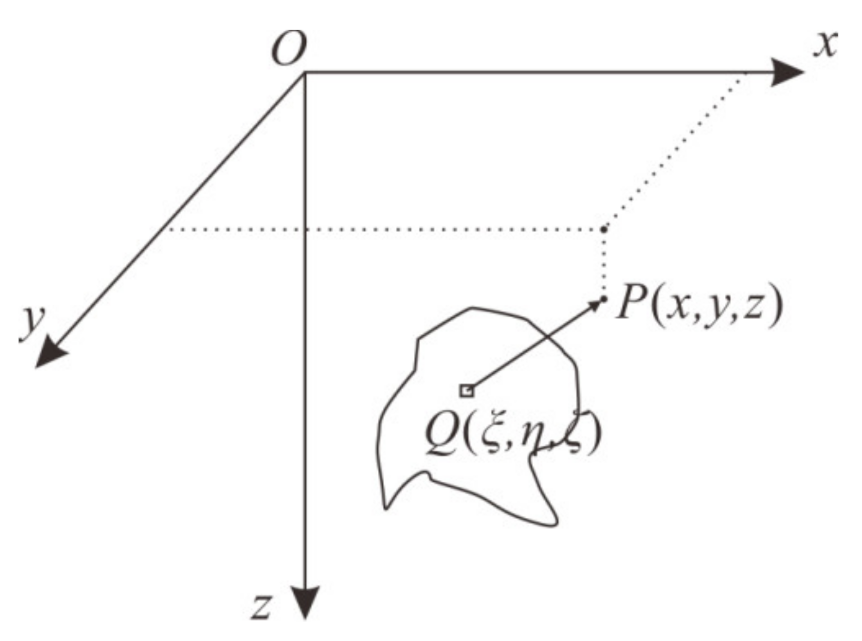
z0) is the center coordinate of the geological body, and (x, y, z) is the coordinate of the observation point.
The first and second order vertical derivatives of gravity anomaly can be defined as:
g x , y , z z = 2 V z 2 = k N z z 0 2 x x 0 2 y y 0 2 x x 0 2 + y y 0 2 + z z 0 2 N + 3 2 ,
and
2 g x , y , z z 2 = 3 V z 3 = k N + 1 z z 0 N z z 0 2 3 x x 0 2 3 y y 0 2 x x 0 2 + y y 0 2 + z z 0 2 N + 5 2 .
The horizontal distance between the zero point of the first vertical derivative and the real position of the geological body can be deduced as:
D 0 , 1 = x x 0 2 + y y 0 2 = N z z 0 .
The horizontal distance between the zero point of the second vertical derivative and the real position of the geological body can be deduced as:
D 0 , 2 = x x 0 2 + y y 0 2 = 3 N z z 0 .
It can be seen from Equations (4) and (5) that the horizontal error of zero value point of different order vertical derivative increases with the depth of the geological body, but the horizontal error of zero value of the second order vertical derivative is larger than that of the first order. Next, we obtain the following equation by making zz0 = 0:
D 0 , 1 = D 0 , 2 = 0 .
Therefore, the zero value points of different order vertical derivatives coincide at position of the geological body (x0, y0, z0), when the distance between the observation height and the geological body is zero (zz0 = 0).
Above, we proved that the zero points of vertical gradients of different orders intersect at the center of the isolated geological body. However, the separate field source is uncommon in actual geological environments. It is more realistic to choose the prism as a geological body model. When the bottom is deep, it can represent intrusive rocks, and when the thickness is small, it can represent rock beds, etc. Therefore, taking the two-dimensional gravity anomaly of prism as an example, the relationship between the prism boundary and the zero value of different vertical derivatives is discussed.
The two-dimensional gravity anomaly of a single prism is defined as:
g x , z = V z = k x + a ln x + a 2 + z H 2 x + a 2 + z h 2 x a ln x a 2 + z H 2 x a 2 + z h 2 + 2 z H tan 1 x + a z H tan 1 x a z H 2 z h tan 1 x + a z h tan 1 x a z h
where, H is the depth of the top surface of the prism, h is the depth of the bottom surface, and a is the horizontal distance from the center to the edge of the prism.
Its first and second vertical derivatives can be expressed as:
g x , z z = 2 V z 2 = 2 k tan 1 z H x + a tan 1 z h x + a tan 1 z H x a + tan 1 z h x a
and
2 g x , z z 2 = 3 V z 3 = 2 k x + a x + a 2 + z h 2 x + a x + a 2 + z H 2 x a x a 2 + z h 2 + x a x + a 2 + z H 2
Then, their zero-point coordinates are:
x 0 , 1 = ± a 2 + z H z h
and
x 0 , 2 = ± 1 6 4 a 2 + z h 2 + z H 2 2 + 12 z h 2 z H 2 + 2 a 2 z h 2 z H 2
When (zh) = 0, we find that the zero-point coordinates of the two vertical derivatives are both, that is the boundary position of the prism top surface:
x 0 , 1 = x 0 , 2 = ± a .
We can calculate the zero-point intersection position of different order vertical derivatives in the lower half space by the following three steps in our method. We will use the Laplace equation for transformation to calculate the higher order derivatives.
  • The original data is continued downward to obtain the three-dimensional data in the lower half space.
In order to reduce the divergence and instability of downward continuation, we use the Taylor series expansion of potential fields for downward continuation in the calculation process (detailed theory is provided in Appendix A), as:
f x , y , h = 2 f x , y , 0 f x , y , h + 2 f x , y , 0 z 2 h 2 + 2 4 ! 4 f x , y , 0 z 4 h 4 + + 2 2 l ! 2 l T x , y , 0 z 2 l h 2 l
where, f (x, y, h) is the downward continuation gravity anomaly h is the depth for downward continuation, and f (x, y, 0) is the gravity anomaly observed on the surface. l is normally 2 or 3, to reduce the instability of the method.
2.
Because the exhibition effect of zero value in the image is not good, two edge detection methods that used zero value of different order derivative to detect geological body boundary are used to find the intersection points of different derivatives.
The first method is normalized tilt angle (TDX), defined as:
T D X = tan 1 V x z 2 + V y z 2 V z z .
Its maximum position corresponds to zero position of the first-order vertical derivative.
The second one is step-edge detection method (SD). Its expression is as follows:
S D = tan 1 V x z 2 + V y z 2 C × V z z z C = m e a n V z z / V z z z
where, C is a parameter in the formula that is used to adjust the amplitude of edge detection result and improve the convergence of the result and make the formula have mathematical significance. The maxima of SD have the same position as the zero value of second order vertical derivative.
3.
Determining the geological body position according to the intersection position.
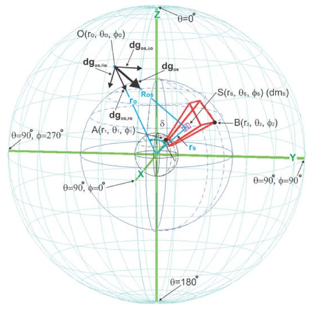
This method mainly aims at the gravity and magnetic anomaly data caused by the underground abnormal body, and is mainly applied to resource exploration and structural division. In general, because the scope of the object is not large, a rectangular coordinate system is adopted and the influence of the earth curvature is ignored. However, the theory of this method is still applicable in a spherical coordinate system; the specific derivation process is shown in Appendix A.

3. Results

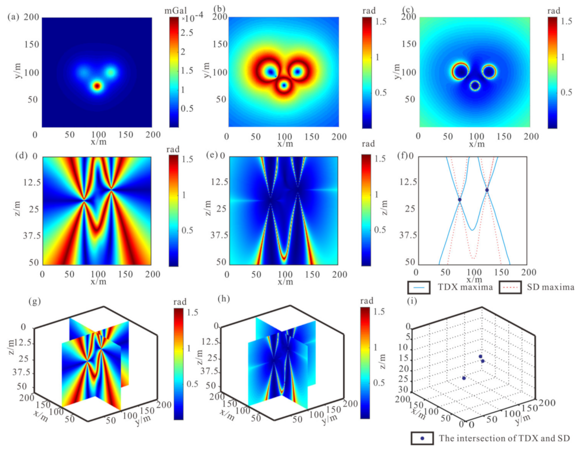
Three spheres with coordinates of x0, y0, 
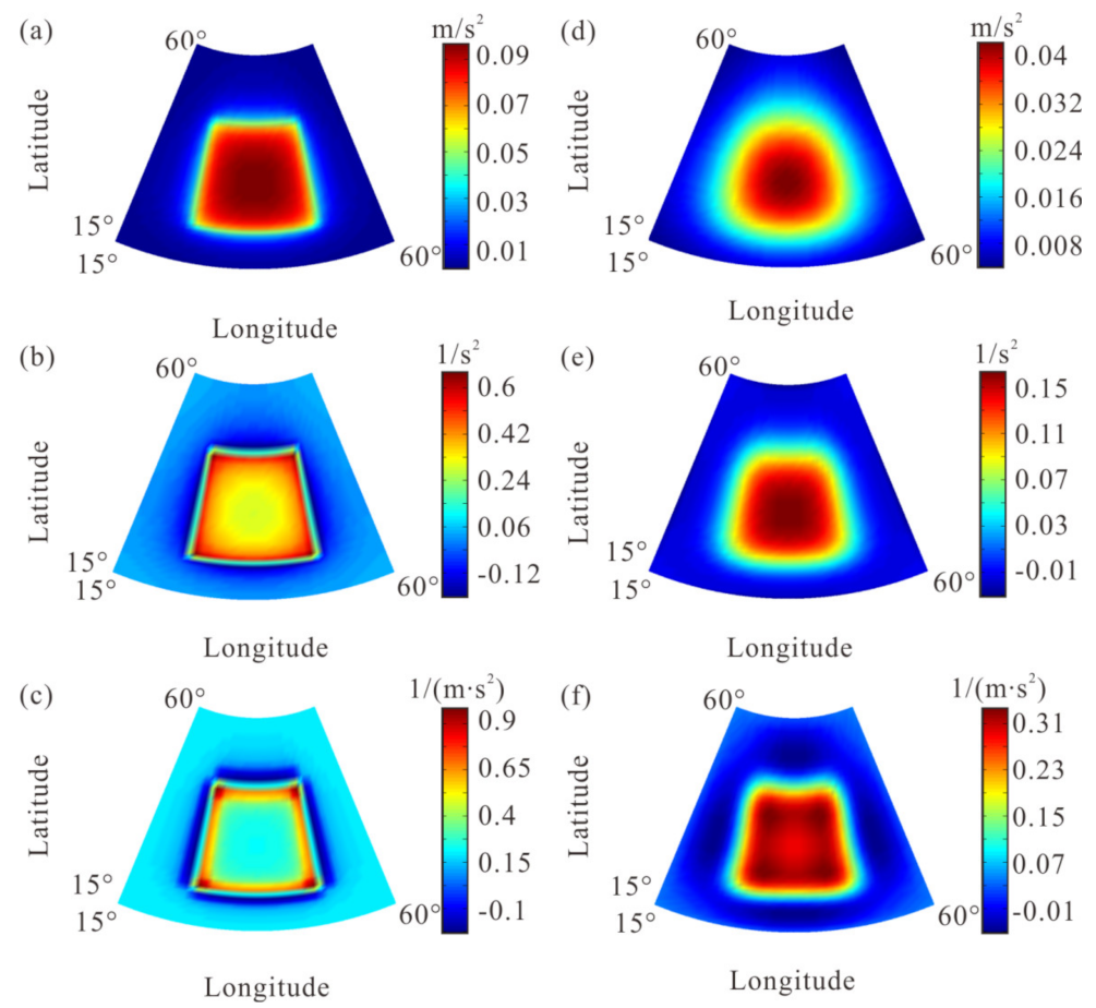
z0 are (75 m, 100 m, 20 m), (125 m, 100 m, 15 m), and (100 m, 75 m, 10 m), respectively. The gravity anomaly is shown in Figure 1a. Figure 1b,c is the TDX and SD edge detection results of anomaly in Figure 1a. It can be seen that the SD result of the sphere model is more convergent than the TDX result. Then, we calculate the spatial results of TDX and SD. To show the imaging results more clearly, we show the slice (x = 100 m) that contains the centers of two spheres. From the slice results, we can see that there are two extremum lines of TDX and SD for each sphere, and the two extremum lines of the two edge detection methods intersect at the center of the sphere (Figure 1d–e). We put the extremum lines of TDX and SD together in Figure 1f, which shows that the intersections of TDX and SD extremum lines are at the centers of the spheres. Figure 1g,h show the spatial TDX and SD results of three-dimensional anomaly in the lower half space, and the slice positions are x = 100 m and y = 100 m, passing through the centers of three sphere models. Three intersection points, obtained by extracting the intersection of two edge detection results, are at the center of the sphere model, which are (75 m, 100 m, 20 m), (125 m, 100 m, 15 m), and (100 m, 75 m, 10 m) (Figure 1i). The sphere model example proves that our method can accurately and quickly obtain the position of geological body.
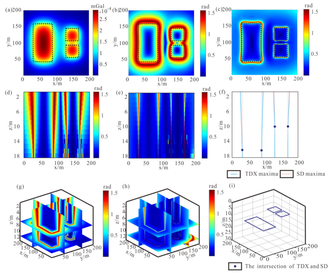
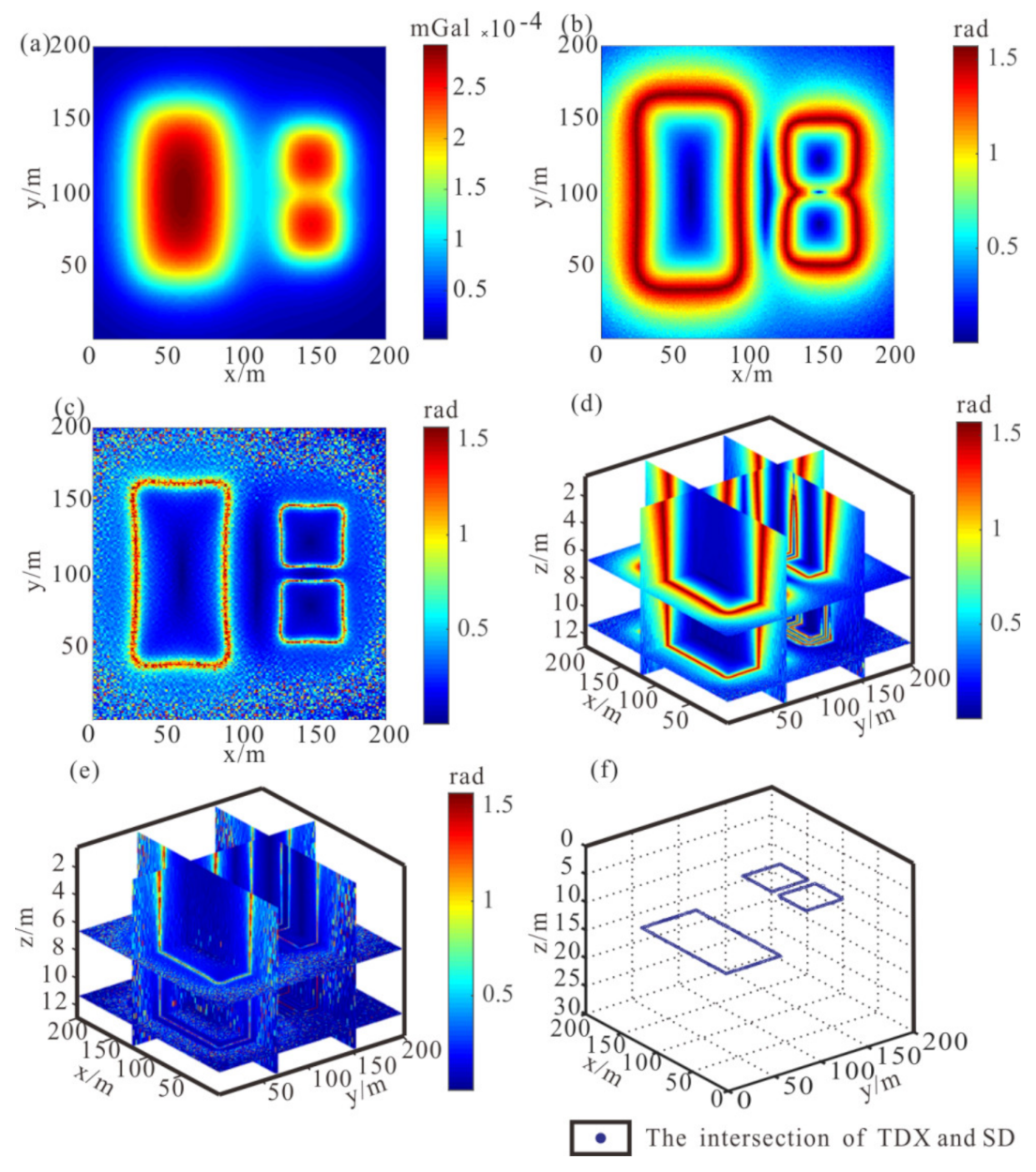
Next, the prism model was established to simulate the complex underground structure. The model parameters are shown in Table 2.
Where, prism 1 represents a deep geological body, prism 2 and 3 represent two geological bodies close to each other. The gravity anomalies of the models are shown in Figure 2a. Figure 2b,c shows the TDX and SD edge detection results of gravity anomaly of the prism model. We can see that the result using TDX is more divergent than the SD, and it cannot distinguish between the boundaries of two geological bodies that are close to each other. In order to present the imaging results more clearly, we show the x = 125 m slice with four edges of two prisms (prism 2 and 3). As shown in Figure 2d–e, it can be seen that we cannot infer an accurate position of prism boundary by referring to the result of single edge detection. Then, the intersection position of the two edge detection results was extracted (Figure 2f). Since the downward continuation depth is deeper than the depth of the model surface, the characteristic value of the different-order derivative continuously intersects below a certain depth; only the first intersection point of each maxima value line will be taken as the result of our method. Although false boundaries are detected in the deep region due to downward continuation, these false boundaries will not produce intersection points and will not affect the accuracy of the method. Figure 2g,h shows the spatial results of TDX and SD in the lower half space. The slice positions in the Figure 2g–h are z = 13 m (top surface of prism 1), z = 8 m (top surface of prism 2 and 3), x = 60 m (passing through prism 1), x = 150 m (passing through prism 2 and 3), and y = 125 m (passing through prism 1 and 3).The ultimate results of the model tests are shown in Figure 2i. It can be seen that the intersection points of characteristic value of different-order vertical derivatives are distributed at the top of three prism boundaries, which proves that our method can effectively determine the edge position of the geological body’s top surface.
To verify the anti-noise capability of our method, the gravity anomaly of prisms model is shown in Figure 3a, which added Gaussian noise with SNR = 70. Figure 3b and Figure 2c show the TDX and SD edge detection results of gravity anomaly with noise. Although the Laplace’s equation is used to calculate the high-order vertical derivative of the anomaly, the SD method is still more affected by noise than the TDX method. Figure 3d,e shows the 3D view of TDX and SD in the lower half space obtained by downward continuation. It can be seen from the figure that both methods are affected by noise with the increase in continuation depth, but the results can still be identified. The intersections position of two edge detection results are extracted and displayed in Figure 3f. Compared with the results shown in Figure 2f, a few imaging results are missing or have small-scale position offset, but they still converge at the boundary of the top surface of prisms overall. The results show this method has a certain degree of anti-noise property. However, to obtain more accurate results, it should be denoised before application.
This section will be divided into subheadings. It should provide a concise and precise description of the experimental results, their interpretation, as well as experimental conclusions that can be drawn.

4. Ore Body Location Inference in Baiyinnuoer-Shuangjianzishan Ore District

4.1. Regional Geology

The Baiyinnuoer-Shuangjianzishan ore district, rich in large-scale Pb-Zn-Ag deposits, is in Balinzuoqi, Inner Mongolia Autonomous Region, China. Based on its geology, mineralogy, geochronology, geochemistry, and geophysics, researchers have made a lot of research on the metallogenic chronology, mineralization, and ore controlling factors of this area, and have achieved important progress. The study area belongs to the Huanggangliang-Ganzhuermiao metallogenic belt, which is in the eastern part of the Central Asian orogenic belt and the southeast part of Daxinganling. This area experienced tectonic evolution thrice and was influenced by three domains: the paleo Asian Ocean tectonic domain, the Mongolia Okhotsk ocean tectonic domain, and the paleo Pacific tectonic domain (Figure 4a). The three subduction events in the whole Mesozoic were conducive to the mineralization in the south of Daxinganling.

4.1.1. Stratigraphy

Most of the strata in the study area have a common feature. The late Paleozoic strata (especially Permian) as the base is covered with Jurassic-Cretaceous continental volcanic rocks, showing a typical two-layer structure. For example, the lower Permian Zhesi formation and Huanggangliang formation in the Baiyinnuoer area are important lithologic and stratigraphic conditions of the deposits. The discovered polymetallic mineralization areas are mostly in or near the Permian strata (in a previous work of our study area), indicating that the strata are closely related to polymetallic mineralization (Figure 4b).

4.1.2. Geological Structure

The study area is located in the superposition of three tectonic domains, which is the junction of the North China plate and Siberian plate and intersection of the xilamulunhe fracture, Erlian-hegenshan fracture, and Nenjiang fracture. It belongs to the eastern part of the Central Asian orogenic belt. The Paleozoic strata in the study area has experienced strong folding. The tectonic location belongs to the Tianshan Xingan geosyncline fold area, the central Inner Mongolia geosyncline fold system, and the late Variscan geosyncline fold belt in Sonid Right Banner. The Huanggang Ganzhuermiao anticline runs through the area in the NE-SW direction, which is closely related to the distribution of regional lead-zinc deposits. Ore controlled by a combination of fractures and folds in this area points to the fact that the junction of fracture and the collapse zone of anticline axis is appropriate for ore bearing. The strata and intrusive rocks controlled by the NE direction Huanggangliang-ganzhuermiao fracture are distributed in the NE direction (Figure 4c).

4.1.3. Magmatism and Metallogenic Model

Magmatic activities are frequent in the southeastern part of Daxinganling, which can be divided into Hercynian, Indosinian, and Yanshanian periods. Baiyinnuoer granodiorite is an Indosinian magmatic intrusive body, which is closely related to skarn type mineralization in the mine area. During the Yanshanian movement, the magmatic activity in the Daxinganling area reached its peak, and it was exposed on a large scale in the central uplift belt of the southeastern segment. The Yanshanian magmatic intrusion in the area is obviously zonal distribution in the NE direction, and its lithology is mainly intermediate acid granite. The leading cause of the large-scale formation of hydrothermal polymetallic deposits is the Yanshanian magmatism. In the southeast part of Daxinganling, there are a large number of ore deposits formed by multi-stage superimposed mineralization. For example, the Shuangjianzishan deposit is a magmatic hydrothermal deposit with two main metallogenic periods of late Jurassic and early Cretaceous. The Baiyinnuoer deposit is a composite deposit with early Cretaceous epithermal vein type Pb-Zn-Ag mineralization superimposed on the Triassic skarn deposit (Figure 4c).

4.1.4. Physical Properties of Rocks

We collected the physical parameters of rock samples in the study area. The density of sedimentary rocks in the area is generally 2.6–2.7 g/cm3, which is high-density. The intrusive rocks are characterized by low density. The average density of granite is 2.55 g/cm3, which is significantly lower than that of sedimentary rocks. The density of the identified ore body is high, up to 6.199 g/cm3.
The magnetic susceptibility of the sedimentary layer in this area is obviously low, about 0.06–0.2 × 10⁻³ SI. The intrusive rocks generally with high magnetic susceptibility, about 1.34–1.70 × 10⁻³ SI. The magnetic susceptibility of the identified ore bodies is the highest, about 50 × 10−3 SI.
Therefore, according to the different responses of different rocks to gravity and magnetic anomalies, the corresponding characteristics of gravity and magnetic fields of different rocks can be summarized (Table 3).
According to the combination characteristics of gravity high-value anomaly and strong magnetic anomaly of ore body, we delineate the metallogenic potential area. The process is as follows (Figure 5).

4.2. Gravity and Magnetic Anomalies Processing

The data used in this paper were measured and processed by the authors’ team in June 2018, and they are 1:5000 scale airborne gravity and aeromagnetic data. The measured direction is northwest and the measured flight altitude is about 100 m. The error of airborne gravity measurement is about 0.62 mGal and that of the aeromagnetic measurement is 2.26 nT. The measured area is 5 × 20 km. Because the horizontal range is small, we will use a rectangular coordinate system for the application of the method. Figure 6a shows the Bouguer gravity anomaly map of the Shuangjianzishan Baiyinnuoer area (the Bouguer gravity anomaly and its physical significance are shown in Appendix A). It can be seen that there is an obvious gravity gradient belt in this area, the strike of gravity anomaly is in the NE direction, and the anomaly rises from West to East. It corresponds to the Huanggangliang Ganzhuermiao anticline—the strike is in the NNE direction).
Figure 6b shows the RTP magnetic anomaly map of the study area. A stripped magnetic anomaly can be seen in Figure 6b—the strike is in the NNE direction. However, the RTP magnetic anomaly does not correspond to the geological structure in this area.
Because the gravity and magnetic anomalies is the comprehensive response of all underground abnormal bodies. In order to obtain the anomalies aimed at research purposes, it is necessary to separate them. The separated regional field is used to divide the regional structure, and the local field is used to delineate the range of metallogenic potential area.
Firstly, the anomalous radial logarithmic power spectrum is obtained. The depth of the field source can be expressed by the slope of the fitting line, as:
h = k / 2 .
where h is the depth of the field source and k is the slope of the straight line.
Then, a filter is established by using the relationship between the slope of the radial logarithmic power spectrum (Figure 7) and the depth of the field source. The anomalies of ore body (residual anomalies of geological bodies with depth of about 250 m) and regional structure (regional anomalies caused by regional tectonics and Moho) are separated, and the noise is removed (Figure 8).

4.3. Structure Division

The fractures in the study area are developed, which play an important role in controlling the intrusion of magma and the occurrence and distribution of metallic minerals. The orebody is mainly controlled by the NE-NNE direction fractures and folds. Therefore, the division of structures is an important task for mineral exploration in this area.
Due to the development of intrusive rocks in the study area, the characteristics of magnetic anomalies are more complex, which do not correspond to the structures in the area. However, the variation in the gravity field usually has a good correspondence with the structure. Therefore, we will use the regional gravity anomaly to divide the structure in the study area.
Figure 9 shows the structure division results of the study area. From the results, we can see the location of the Huanggangliang-Ganzhuermiao anticline, and divide the distribution of fractures in the study area. The fracture strike is in the NE, NW, and NS direction, and the NE direction fractures are more developed.

4.4. Delineation of Metallogenic Potential Area

Next, we delineate the metallogenic potential area of the study area. The initial boundary detection results were obtained by applying the SD method to the residual gravity anomaly, and the results correspond well to the anomaly (Figure 10). It has been proved that the accuracy of the edge detection method is affected by the depth of the field source. Therefore, we will use the SDD method to obtain the accurate distribution and depth of the orebody.
Before applying our method, it is necessary to obtain the anomaly in the lower half space by downward continuation. According to the relationship between the radial logarithmic power spectrum and the depth of the field source, the anomaly of the separated ore body should be extended downward by 600 m in 10 m steps. After the lower half space gravity anomalies are obtained, TDX and SD methods are respectively applied to gravity anomalies on different observation surfaces to obtain the detection results of TDX and SD in a three-dimensional space (Figure 11). We will take the x = 5 km profile as an example to show the results of our method and carry out further explanation. There are 21 intersection points that can be seen from the imaging results, which correspond to 21 boundaries of the geological anomalous bodies in this profile, with depths approximately between 200 m and 400 m. Finally, we delineated the favorable metallogenic areas (orange and red range) on this profile by combining the profile anomalies and intersection points.
The inversion results of the whole area are summarized and uniformly displayed on the plane to obtain the distribution of medium and high-density bodies in the area, which can be inferred to as sedimentary rock and orebody. These medium and high-density bodies are distributed around the fractures in the region and have close contact with intrusive rocks (Figure 12a).
Next, we applied the SDD method on the RTP magnetic anomaly after separation in the study area. The distribution of medium- and high-susceptibility rocks in the region, which are considered intrusive rocks and orebodies, is obtained (Figure 12b). The high magnetic rock mass is mostly distributed on the fracture location, which proves that the fractures in the area provide a channel for magmatic intrusion and have an important influence on mineralization in this area.
The high-density range and high susceptibility range are superimposed to obtain a range consistent with the combined characteristics of the orebody (Table 3). It is the contact zone between intrusive rocks and sedimentary rocks, shown in purple, which is inferred to be the metallogenic potential area in the study area (Figure 12c). In addition, there are two mines already in production in the study area, which are located in our inferred potential area. Therefore, we believe that our work will lay the foundation for subsequent exploration.

5. Conclusions

In this paper, the relationship between the horizontal positions of the characteristic values of different vertical gradients (0 values) of gravity and magnetic anomalies and the depth of the anomalous bodies is derived. We propose the field source position imaging method using intersections of gravity and magnetic different-order derivatives. In this method, two edge detection methods are introduced to find the intersection position of the lower half space to determine the exact position of the anomalous body. The results of various model tests show that this method offers high resolution and high applicability. Our method uses the horizontal iterative method of stable downward continuation, and uses the Laplace equation to calculate the high-order vertical derivatives of gravity and magnetic anomalies to suppress noise interference, so that the method has good noise resistance.
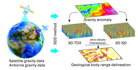
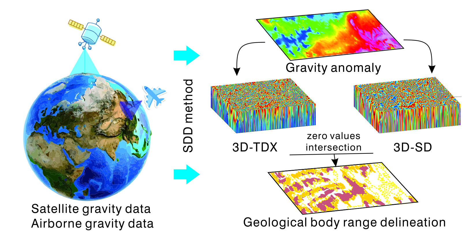
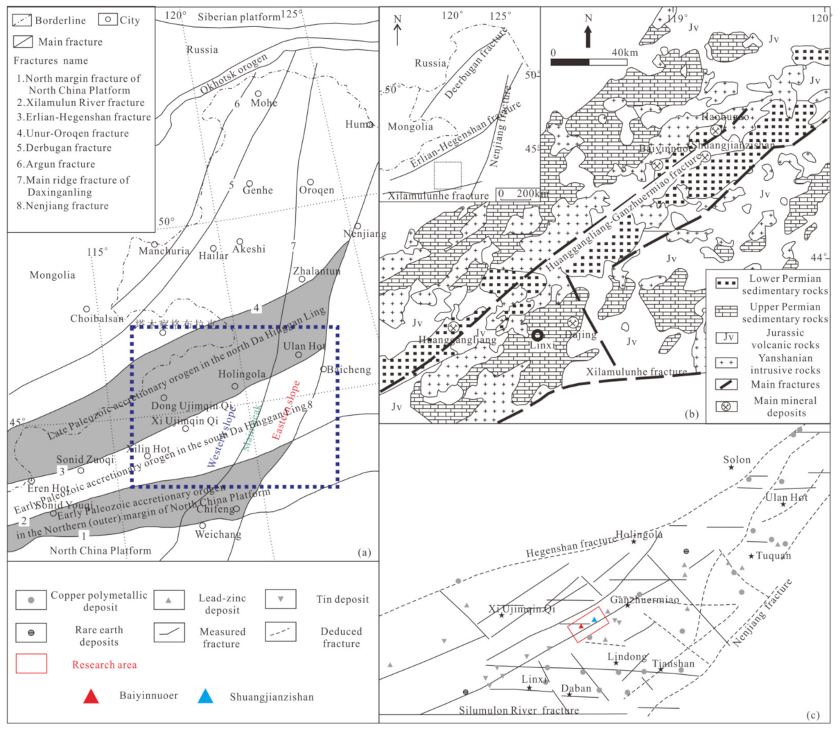
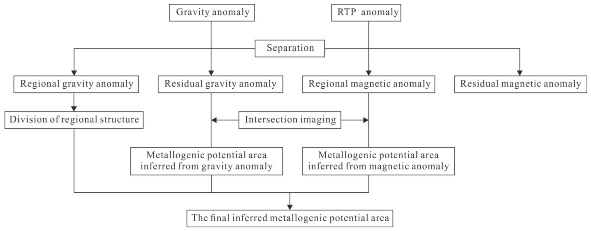
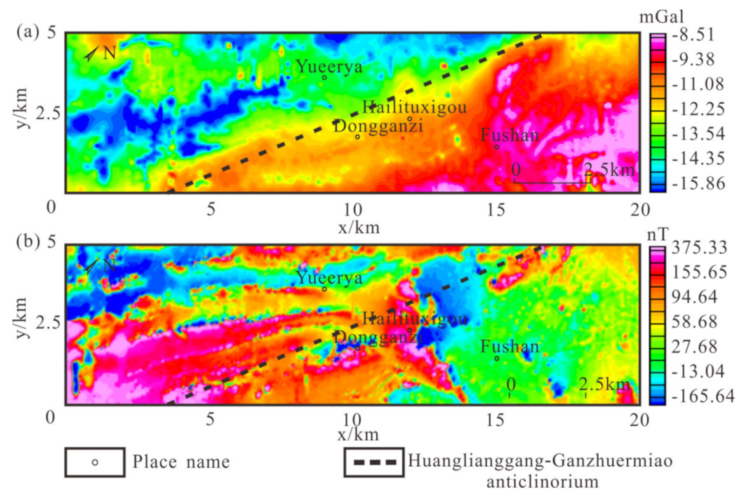
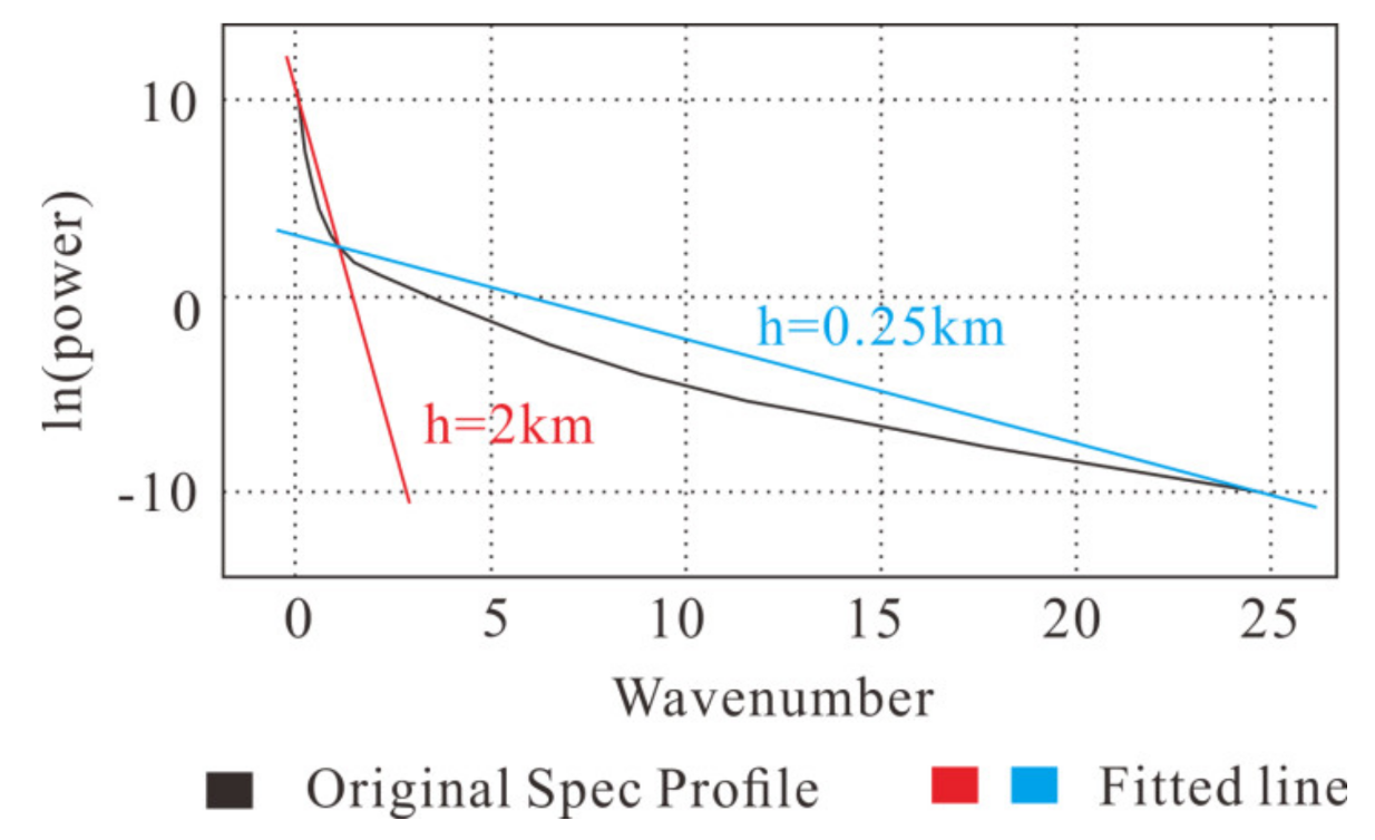
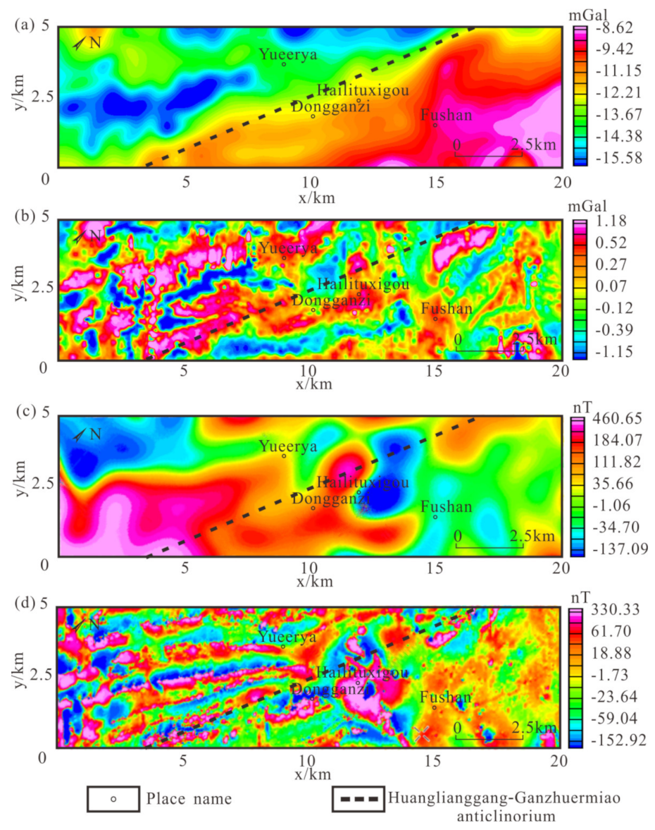
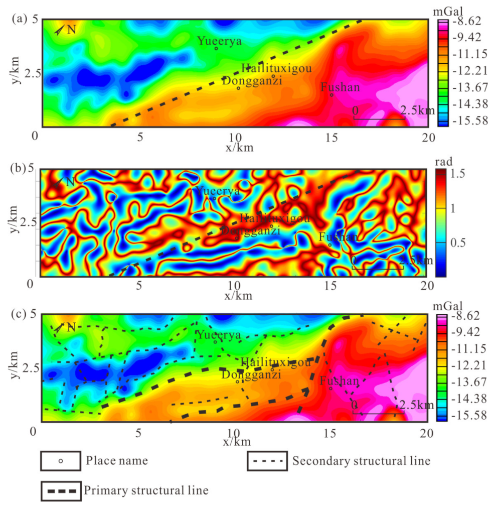
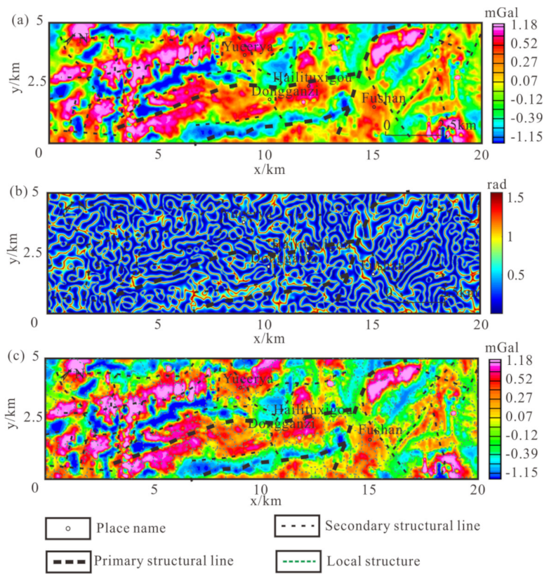
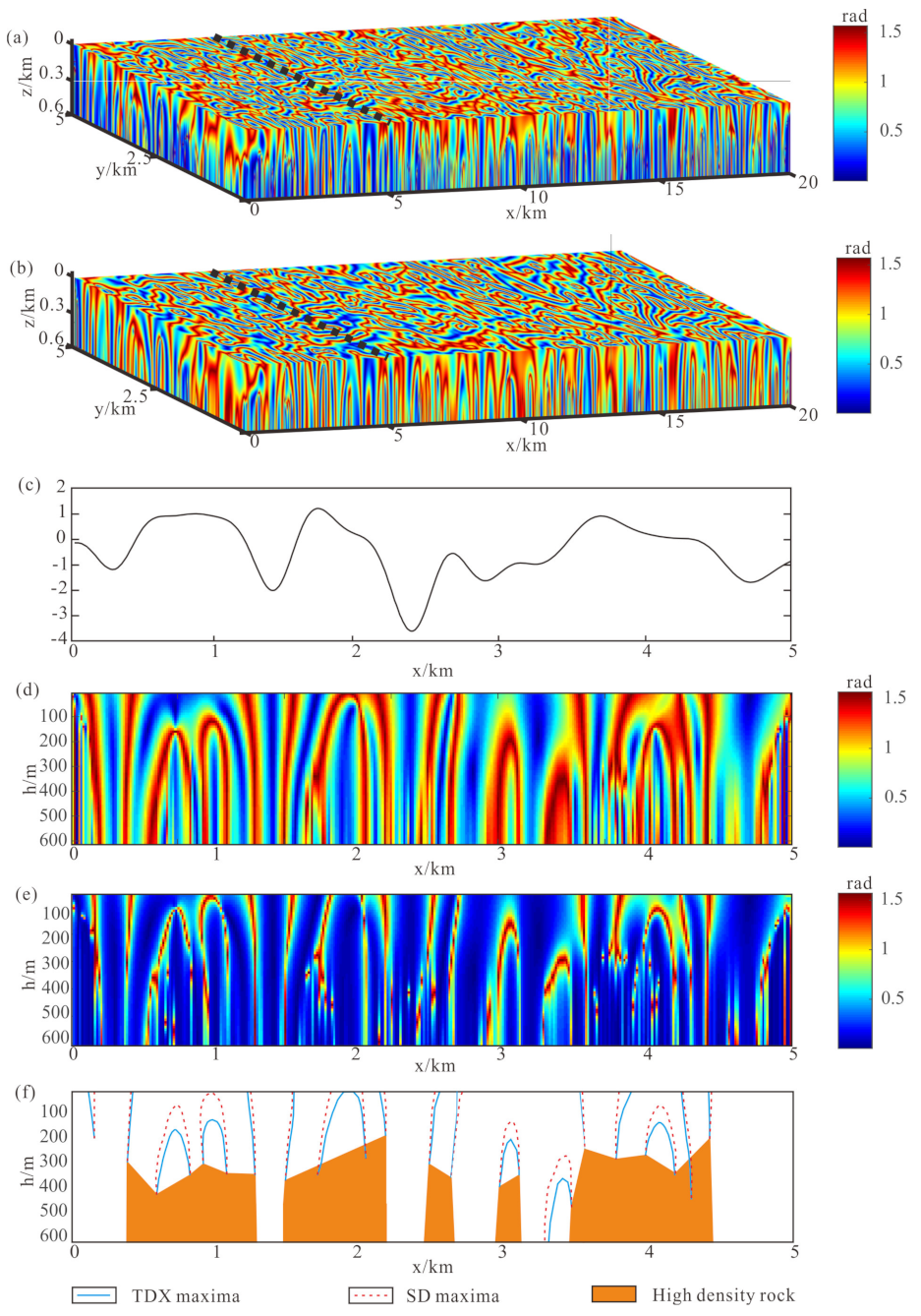
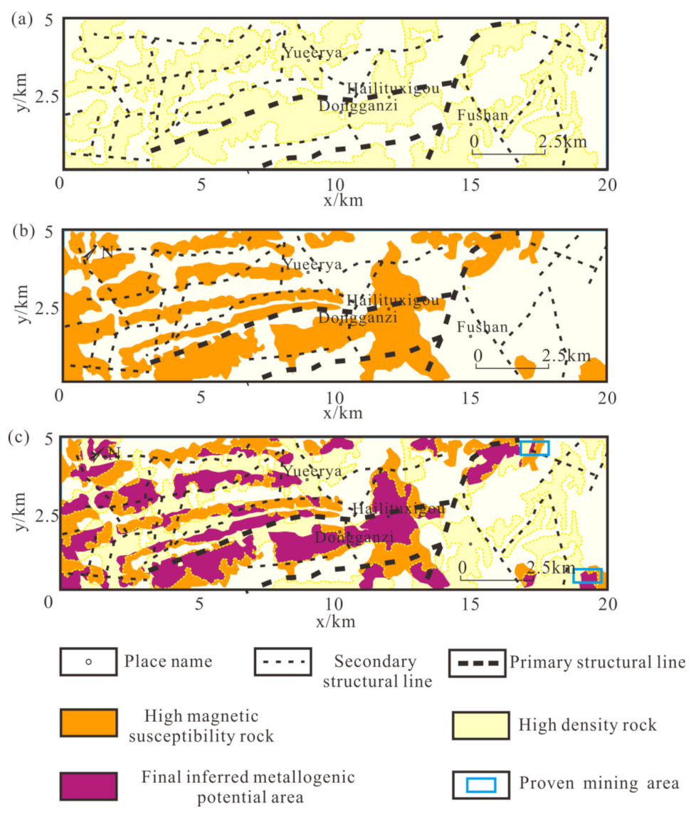
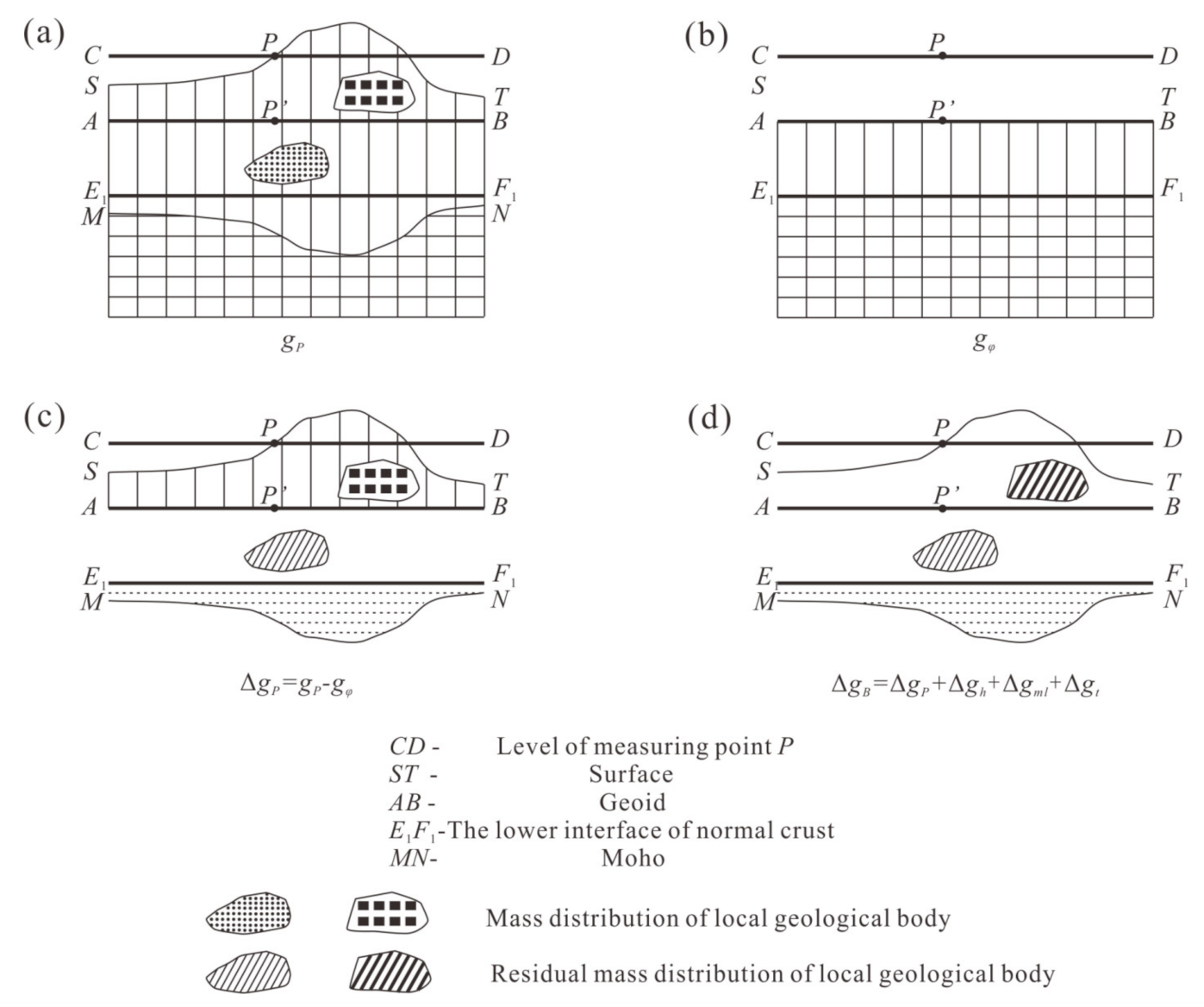
Next, we process and interpret the measured airborne gravity data and aeromagnetic data in the Baiyinnuoer–Shuangjianzishan area. We separated regional anomalies (reflecting deep structure) and residual anomalies (reflecting shallow geological body) by using the field separation method in wave number domain. The SD edge detection method is applied to gravity regional anomaly, the specific location of Huanggangliang-Ganzhuermiao anticlinorium is determined, and other secondary structures are divided. The overall strike of the structure in the region is NNE. By analyzing the gravity and magnetic residual anomalies, we can see that the anomalous bodies are generally distributed around the divided structures, which indicates that the magmatic movement is frequent in the region, and the structures provide channels for magmatic intrusion that supplies sufficient material basis for metallogeny. The SSD method was used to circle the high magnetic susceptibility and high-density range for residual gravity and magnetic anomalies. Combined with the known combination of gravity and magnetic response of rocks in the study area, the range of metallogenic potential area in the area was finally deduced. The depth of ore bodies in this area is about 200–400 m, and they are concentrated in the southwest of the research area. In addition, their strike is roughly consistent with the structure in the area, which is in the NE direction. In the eastern part of the study area, two ore fields have been produced, which are in the range of the metallogenic potential area delineated in this paper, proving that the results of this paper are accurate and lay a foundation for further exploration.

Author Contributions

Conceptualization, Y.M. and G.M.; methodology, Y.M.; software, L.L.; validation, T.W., J.H., and G.M.; formal analysis, G.M.; investigation, L.L.; resources, J.H.; data curation, J.H.; writing—original draft preparation, Y.M.; writing—review and editing, Y.M.; visualization, Y.M.; supervision, G.M.; project administration, G.M.; funding acquisition, J.H. All authors have read and agreed to the published version of the manuscript.

Funding

This research was funded by the National Natural Science Foundation of China (42074147), The National Key Research and Development Program Issue During the 13th Five-year Plan Period (2017YFC0602203; 2017YFC0601606; 2017YFC0601305), and The Excellent Young Talents Fund Project of Jilin Province (20190103011JH).

Data Availability Statement

The data presented in this study are available on request from the corresponding author.

Conflicts of Interest

The authors declare no conflict of interest.

Appendix A

A.1. Gravity Anomaly and Its Physical Significance

It is assumed that there is a spherical ore body underground near point P on the geoid (Figure A1). The density of the ore body is ρ1 and the volume is v. If the density of surrounding rock is ρ2, the residual density of ore body relative to surrounding rock is ρ = ρ1 − ρ2 (when ρ1 > ρ2, ρ1 > 0, and when ρ1 > ρ2, ρ1 < 0), and the residual mass of ore body is m = ρv.
Figure A1. Physical significance of gravity anomaly.
Remotesensing 13 00964 g0a1
If the normal gravity is gφ and the gravity of the residual density of the ore body is F (pointing to the center of the ore body), then the actual gravity of point P is g = gφ + F. As shown in the figure, the gravity anomaly of point P is defined as:
Δ g =   g     g φ   = g g φ .
From the cosine theorem, we have:
g = g φ 2 + 2 g φ F cos θ + F 2 1 / 2 ,
where, θ is the angle between F and gφ. Taking Equation (A2) into Equation (A1), we can get:
Δ g + g φ = g φ 2 + 2 g φ F cos θ + F 2 1 / 2 .
Divide the square of the Equation (A3) by gφ2 to get Equation (A4), as:
Δ g g φ 2 + 2 Δ g g φ = F g φ 2 + 2 F g φ cos θ .
Because F << gφ, (Δg/gφ)2 and (F/gφ)2 are negligible. We can get:
Δ g = F cos θ .
The above equation shows that the physical meaning of gravity anomaly is the component of gravity produced by residual mass in the normal gravity direction (or in vertical direction). It should be noted that the gravity anomaly is not the gravity of the residual mass itself (except point O). Because the gravity of the residual mass is far less than normal gravity, the gravity of the residual mass basically does not change the direction of gravity.
The actual gravity anomaly is usually composed of two parts, namely:
Δ g = Δ g 1 + Δ g 2 .
where, Δg1 is regional gravity anomaly (large-scale gravity anomaly) and Δg2 is residual gravity anomaly (small-scale gravity anomaly). Assume that the residual density of underground abnormal body is evenly distributed. As shown in Figure A2, take a point o on the ground as the coordinate origin, the z-axis is vertically downward, that is, along the gravity direction, and the x and y-axes are in the horizontal plane. The gravitational potential of the underground abnormal body is as follows:
V = G ρ v d v r = G ρ v d ξ d η d ζ x ξ 2 + y η 2 + z ζ 2 1 / 2 .
From the above equation, the basic integral expression of gravity anomaly is obtained as follows:
Δ g = V z = G ρ v z ζ d ξ d η d ζ x ξ 2 + y η 2 + z ζ 2 3 / 2 .
Figure A2. Gravitational potential and field of the geological body.
Remotesensing 13 00964 g0a2

A.2. Bouguer Gravity Anomaly and Its Physical Significance

Although we can use the instrument to measure the gravity difference between each measuring point and the base point, there are many factors that cause the difference between each measuring point and the base point. In addition to the underground geological factors, there is also the normal field difference, the elevation difference, and the terrain rise and fall around the measuring point. In order to obtain the gravity anomaly only caused by underground geological factors, it is necessary to correct the data. Bouguer gravity anomaly is a kind of gravity anomaly after normal field correction, height correction, middle layer correction, and terrain correction, which is expressed as:
Δ g B = g P g φ + Δ g h + Δ g m l + Δ g t .
where, gP is the observed gravity of the observation point P, gφ is the normal gravity field, Δgh is the height correction, Δgml is the middle layer correction, and Δgt is the terrain correction.
Next, we illustrate the geological geophysical significance of the Bouguer gravity anomaly with the crustal structure shown in Figure A2.
Figure A3a shows the earth structure around the survey point P, P′ is the projection of the point P on the geoid, and gP is the absolute gravity of P; Figure A3b shows the crustal structure assumed in the derivation of the normal gravity formula, and gφ is the normal gravity of the survey point P′. The normal field correction of point P is ΔgP = gPgφ. From the crustal structure, the normal field correction is Figure A3a minus Figure A3b (as shown in Figure A3c). The mass distribution above AB is consistent with that in Figure A3a, but there is only local residual mass between AB and E1F1, and there is a relative mass deficit between E1F1 and MN. After height correction, the difference of normal field caused by height between point P and P′ is eliminated. After terrain correction and middle layer correction, the mass of normal crustal density above AB is removed, but the local residual mass exists. Therefore, the Bouguer gravity anomaly reflects all kinds of geological bodies in the crust, which deviate from the normal crustal density.
Figure A3. Geological and geophysical significance of various gravity anomalies. (a) Absolute gravity of P; (b) Normal gravity field; (c) Correction of normal gravity field; (d) Bouguer gravity.
Remotesensing 13 00964 g0a3

A.3. Processing and Transformation of Gravity Anomaly in Wavenumber Domain

The basic formula of gravity data processing and conversion in space domain can be written as the following convolution form:
f b x , y , z = f a x ξ , y η , 0 φ x , y , z d ξ d η .
where, fa and fb represent the original exception and the processed exception, respectively, and φ is the weight function. Although there are many different conversion forms of gravity anomaly, different processing and conversion only have different weight functions.
By Fourier transform of Equation (A11), we get:
F ˜ b u , v , z = F ˜ a u , v , 0 φ ˜ u , v , z .
For the upward continuation calculation of gravity anomaly, the integral expression is as follows:
f x , y , z = z 2 π f ξ , η , 0 x ξ 2 + y η 2 + z 2 3 / 2 d ξ d η .
It is known that the convolution in spatial domain corresponds to the product in wavenumber domain. Fourier transform the equation so that the Fourier transform of f x , y , z is F ˜ u , v , z and the Fourier transform of f x , y , 0 is F ˜ u , v , 0 ,and there is:
1 2 π z x ξ 2 + y η 2 + z 2 3 / 2 FT e z u 2 + v 2 .
Therefore, the spectrum of gravity anomaly on observation plane z can be expressed as:
F ˜ u , v , z = F ˜ u , v , 0 e z u 2 + v 2 .
The above equation holds when z is greater than or equal to 0. Its inverse Fourier transform is:
f x , y , z = F ˜ u , v , 0 e z u 2 + v 2 e i u x + v y d u d v .
where, φ ˜ z = e z u 2 + v 2 is called upward continuation factor.
The above formula shows that the gravity anomaly at a certain height in the upper half space can be obtained by calculating the Fourier transform of the gravity anomaly on the z = 0 plane, multiplying it by the continuation factor, and then calculating its inverse Fourier transform.
We can also prove that Equations (A11) and (A12) can be extended to 0< z < H space (H is the field source depth), that is, if the gravity on the z = 0 plane is known, it will be multiplied by the continuation factor, and then the inverse Fourier transform of the product result will be obtained. However, downward continuation in the wavenumber domain will enlarge the high frequency part of the anomaly, resulting in computational instability.
Using the differential theorem to calculate the differential (x, y or z) of Equation (A15), the spectral expression of gravity anomaly derivative can be obtained:
n x n n y n n z n f x , y , z = F ˜ u , v , 0 i u n i v n u 2 + v 2 n e z u 2 + v 2 e i u x + v y d u d v .
where n = 1, 2, … is the order of the derivative.
The derivative factor can be expressed as:
φ ˜ d = i u n i v n u 2 + v 2 n .
where, (iu)n, (iv)n and u 2 + v 2 n are the factors to calculate the n-th derivative in different directions of x, y, and z, respectively.

A.4. The Stable Taylor Series Method of Upward Continuation

Downward continuation is widely used in gravity and magnetic data processing. It includes the equivalent source method, Wiener filter method, singular value decomposition method, downward continuation in wavenumber domain, and Taylor series method, among others. In this paper, we choose the stable Taylor series method of upward continuation.
The Taylor expansion of gravity anomaly on the interface with a certain depth of h is as follows:
g ( x , y , h ) = g ( x , y , 0 ) + g z h + 1 2 ! 2 g z 2 h 2 + 1 3 ! 3 g z 3 h 3 + + 1 m ! m g z m h m .
where, g(x, y, h) is the anomaly on the observation plane h, h is the depth of downward continuation, and g(x, y, 0) is the anomaly on the observation plane.
Similarly, the Taylor expansion of upward continuation is as follows:
g ( x , y , h ) = g ( x , y , 0 ) g z h + 1 2 ! 2 g z 2 h 2 1 3 ! 3 g z 3 h 3 + + 1 m ! m g z m h m .
where g(x, y, −h) is the anomaly on the observation plane −h. We add Equations (A20) and (A21) to get:
g ( x , y , h ) = 2 g ( x , y , 0 ) g ( x , y , h ) + 2 2 ! 2 g z 2 h 2 + 2 4 ! 4 g z 4 h 4 + + 2 2 l ! 2 l g z 2 l h 2 l .
Through the above transformation, we can obtain the Taylor series method using upward continuation. As the value of vertical derivative decreases with the increase of order, we usually choose the fourth derivative to complete the calculation of downward continuation (Equation (A21)):
g ( x , y , h ) = 2 g ( x , y , 0 ) g ( x , y , h ) + 2 2 ! 2 g z 2 h 2 + 2 4 ! 4 g z 4 h 4 .
Since the calculation of vertical derivatives in wavenumber domain will increase the interference of noise, we use the Laplace equation to calculate the second and fourth order vertical derivatives:
2 g z 2 = 2 g x 2 + 2 g y 2 .

A.5. The Stable Taylor Series Method of Upward Continuation

As an effective anomaly analysis method, the spectrum analysis of gravity and magnetic data is widely used in gravity and magnetic data processing, which can effectively analyze the anomaly characteristics and separate the anomalies of different depths.
The power spectrum function P at any depth h can be expressed as:
P = l e r h ,
where l is the factor related to the density, the shape of the geological body, and so on, r = u 2 + v 2 is the radial circular frequency.
Take logarithm of both sides of Equation (A23) to obtain:
l n P = l n l 2 h r .
lnP is called the logarithmic radial power spectrum. It can be seen that there is a linear relationship between the radial logarithmic power spectrum and the radial frequency, and the slope of the line is −2h. Therefore, a fitting line can be obtained from the radial logarithmic power spectrum, as shown in the figure. According to the slope of this line, the buried depth of field source can be calculated as:
h = ln P r 1 ln P r 2 2 r 1 r 2 ,
Therefore, according to the characteristics of the radial logarithmic power spectrum (Figure A4), we can separate the gravity anomalies at different depths by using an appropriate filter.
Figure A4. Radial logarithmic power spectrum.
Remotesensing 13 00964 g0a4

A.6. Gravity Effects for a Spherical Prism

Assuming that the spherical prism in a spherical coordinate system is shown in Figure A5, the displacement distance Ros is given by:
R o s = r 0 2 + r s 2 + 2 r 0 r s cos δ 1 2 cos δ = cos θ 0 cos θ s + sin θ 0 sin θ s cos φ 0 φ s ,
Figure A5. Spherical geometry for modelling at the observation point O(ro, θo, φo) the gravity effects of the spherical prism by integrating the differential source mass dms through the volume of the prism with bottom and top surfaces that include the representative corner points A(r1, θ1, φ1) and B(r2, θ2, φ2),respectively. The Cartesian perspective is given by the superposed, co-registered X, Y, and Z axes (Reference from [21]).
Remotesensing 13 00964 g0a5
Its gravity potential can be expressed as:
P = φ s = φ 1 φ 2 θ s = θ 1 θ 2 r s = r 1 r 2 k R o s d r s d θ s d φ s k = G ρ s r s 2 sin θ s
Then we can obtain the radial gravity anomaly and its first and second derivatives:
g o , r o = φ s = φ 1 φ 2 θ s = θ 1 θ 2 r s = r 1 r 2 k r o + r s cos δ R o s 3 d r s d θ s d φ s ,
g o , r o r o = φ s = φ 1 φ 2 θ s = θ 1 θ 2 r s = r 1 r 2 k R o s 2 + 3 r o r s cos δ 2 R o s 5 d r s d θ s d φ s
g o , r o r o = φ s = φ 1 φ 2 θ s = θ 1 θ 2 r s = r 1 r 2 3 k r o r s cos δ 5 r s 2 cos 2 δ + 4 r o r s cos δ + 3 r s 2 2 r o 2 R o s 7 d r s d θ s d φ s
Because the integrand is an analytic function, it is daunting to find the analytic interpretation of the function compared with the numerical integration. Therefore, the Gauss Legendre integral is usually used for forward calculation of the spherical prism:
r 2 r 1 θ 2 θ 1 φ 2 φ 1 8 n k = 1 K n j = 1 J n i = 1 I A n i A n j A n k f r o , θ o , φ o , r ^ n i , θ ^ n j , φ ^ n k ,
Here, the Gauss-Legendre coefficients (Ani, Anj, Ank) correspond to the coordinates (rni, θnj, φnk) of the n-th Gaussian node in the interval (−1, 1). Each node is the coordinate for a zero of the nth-order Legendre polynomial that orthogonally spans the unit interval.
Because there is no strict analytical solution for spherical prisms, it is impossible to prove our theory in a spherical coordinate system through formula derivation. Therefore, we analyze the different order radial derivatives of spherical prisms on different observation surfaces.
We assume a spherical prism model with a residual density of 1 g/cm3; the specific location parameters are shown in Table A1. We conduct forward modeling for different data of the model, and the results are shown in Figure A6.
Table A1. Location parameters of the spherical prism model
Location Parameters
r14000 km
r25000 km
θ126.25°
θ248.75°
ϕ126.25°
ϕ248.75°
Figure A6. (a), (b) and (c) are gravity anomaly, the first-order radial derivative and the second-order radial derivative at r0 = 5000 km; (d), (e) and (f) are gravity anomaly, the first-order radial derivative and the second-order radial derivative at r0 = 6000 km.
Remotesensing 13 00964 g0a6
In order to more clearly show the relationship between the 0 value of different order derivatives and the model boundary, we extracted the level = 0 contours (Figure A7). When the observation surface is on the top surface of the spherical prism, the 0 values of different order radial derivatives correspond to the boundary of the spherical prism. When the observation surface is above the spherical prism, they all have different degrees of position offset. Thus, we believe the method can be applied to gravity data in a spherical coordinate system.
Figure A7. (a) Zero value lines of different radial derivatives of gravity at r0 = 5000 km; (b) Zero value lines of different radial derivatives of gravity at r0 = 6000 km.
Remotesensing 13 00964 g0a7

References

  1. Evjen, H.M. The place of the vertical gradient in gravitational interpretations. Geophysics 1936, 1, 127–136. [Google Scholar] [CrossRef]
  2. Cordell, L. Gravimetric expression of graben faulting in Santa Fe Country and the Espanola Basin, New Mexico. In Proceedings of the New Mexico Geological Society Guidebook, 30th Field Conference; New Mexico Geological Society: Socorro, NM, USA, 1979; pp. 59–64. [Google Scholar]
  3. Miller, H.G.; Singh, V. Potential field tilt—A new concept for location of potential field sources. J. Appl. Geophys. 1994, 32, 213–217. [Google Scholar] [CrossRef]
  4. Wijns, C.; Perez, C.; Kowalczyk, P. Theta map: Edge detection in magnetic data. Geophysics 2005, 70, 39–43. [Google Scholar] [CrossRef]
  5. Cooper, G.R.J.; Cowan, D.R. Enhancing potential field data using filters based on the local phase. Comput. Geosci. 2006, 32, 1585–1591. [Google Scholar] [CrossRef]
  6. Cooper, G.R.J.; Cowan, D.R. Edge enhancement of potential-field data using normalized statistics. Geophysics 2008, 73, H1–H4. [Google Scholar] [CrossRef]
  7. Cooper, G.R.J.; Cowan, D.R. A generalized derivative operator for potential field data. Geophys. Prospect. 2011, 59, 188–194. [Google Scholar] [CrossRef]
  8. Ma, G.; Huang, D.; Liu, C. Step-Edge Detection Filters for the Interpretation of Potential Field Data. Pure & Appl. Geophys. 2016, 173, 795–803. [Google Scholar]
  9. Thompson, D.T. EULDPH: A new technique for making computer-assisted depth estimates from magnetic data. Geophysics 1982, 47, 31–37. [Google Scholar] [CrossRef]
  10. Thurston, J.B.; Smith, R.S. Automatic conversion of magnetic data to depth, dip, and susceptibility contrast using the SPI (TM) method. Geophysics 1997, 62, 807–813. [Google Scholar] [CrossRef]
  11. Salem, A.; Ravat, D.; Smith, R.; Ushijima, K. Interpretation of magnetic data using an enhanced local wavenumber (ELW) method. Geophysics 2005, 70, L7–L12. [Google Scholar] [CrossRef]
  12. Werner, S. Interpretation of Magnetic Anomalies at Sheet-Like Bodies. Sver. Geol. Unders. 1953, 57, 447–459. [Google Scholar]
  13. Patella, D. Introduction to ground surface self-potential tomography. Geophys. Prospect. 1997, 45, 653–681. [Google Scholar] [CrossRef]
  14. Patella, D. Self-potential global tomography including topographic effects. Geophys. Prospect. 1997, 45, 843–863. [Google Scholar] [CrossRef]
  15. Mauriello, P.; Patella, D. Localization of maximum-depth gravity anomaly sources by a distribution of equivalent point masses. Geophysics 2001, 66, 1431–1437. [Google Scholar] [CrossRef]
  16. Березкин, B.M. Πрименение Гравиразведки для Поисковместо Рождений не Фти и Газа; Soviet Union: Moscow, Russia, 1973. [Google Scholar]
  17. Aghajani, H.; Moradzadth, A.; Aydin, A. Using Normalized Full Gradient Method to Interpret Gravity Anomalies on Synthetic and Field Data. SGEM 2009, 14, 725–734. [Google Scholar]
  18. Fedi, M. DEXP: A fast method to determine the depth and the structural index of potential fields sources. Geophysics 2007, 72, I1–I11. [Google Scholar] [CrossRef]
  19. Abbas, M.A.; Fedi, M.; Florio, G. Improving the local wavenumber method by automatic DEXP transformation. J. Appl. Geophys. 2014, 111, 250–255. [Google Scholar] [CrossRef]
  20. Abbas, M.A.; Fedi, M. Automatic DEXP imaging of potential fields independent of the structural index. Geophys. J. Int. 2014, 199, 1625–1632. [Google Scholar] [CrossRef]
  21. Asgharzadeh, M.F.; Von Frese, R.R.; Kim, H.R.; Leftwich, T.E.; Kim, J.W. Spherical prism gravity effects by Gauss-Legendre quadrature integration. Geophys. J. Int. 2007, 169, 1. [Google Scholar] [CrossRef] [Green Version]
Figure 1. Imaging results of spatial different order derivative method of sphere model: (a) Gravity anomaly of sphere model on surface; (b) TDX result of gravity anomaly; (c) SD result of gravity anomaly; (d) TDX result of gravity anomaly in the lower half space; (e) SD result of gravity anomaly in the lower half space; (f) Slice results of SDD; (g) x = 100 m slice of TDX 3D result; (h) x = 100 m slice of SD 3D result; (i) imaging results of x = 100 m slice.
Remotesensing 13 00964 g001
Figure 2. Imaging results of different-order vertical derivatives intersection of the prisms model: (a) Gravity anomaly of the prisms model on surface; (b) TDX result of gravity anomaly; (c) SD result of gravity anomaly; (d) TDX result of anomaly by downward continuation in the lower half space; (e) SD result of anomaly by downward continuation in the lower half space; (f) Imaging results of SDD; (g) x = 125 m slice of TDX 3D result; (h) x = 125 m slice of SD 3D result; (i) Imaging results of x = 125 m slice.
Remotesensing 13 00964 g002
Figure 3. Imaging results of different-order vertical derivatives intersection of the noisy model: (a) Gravity anomaly of prisms model with SNR = 70 noise on the surface; (b) TDX result of gravity anomaly; (c) SD result of gravity anomaly; (d) TDX result of anomaly by downward continuation in the lower half space; (e) SD result of anomaly by downward continuation in the lower half space; (f) Imaging results of SDD.
Remotesensing 13 00964 g003
Figure 4. (a) Tectonic pattern in the southern part of Daxinganling; (b) Geological map; (c) Mineral distribution.
Remotesensing 13 00964 g004
Figure 5. Flow chart of metallogenic potential area delineation.
Remotesensing 13 00964 g005
Figure 6. (a) Bouguer gravity anomaly in the Shuangjianzishan Baiyinnuoer area; (b) RTP magnetic anomaly in the Shuangjianzishan Baiyinnuoer area.
Remotesensing 13 00964 g006
Figure 7. Radial logarithmic power spectrum.
Remotesensing 13 00964 g007
Figure 8. Field separation results of Bouguer gravity anomaly and RTP magnetic anomaly: (a) Regional gravity anomaly; (b) Residual gravity anomaly; (c) Regional magnetic anomaly; (d) Residual magnetic anomaly.
Remotesensing 13 00964 g008
Figure 9. Structure division of the study area: (a) Regional anomaly of the study area; (b) the SD result; (c) the result of structure division.
Remotesensing 13 00964 g009
Figure 10. Preliminary division results of local structures in the study area: (a) Residual anomaly in the study area; (b) SD results of residual anomaly; (c) Structure division results.
Remotesensing 13 00964 g010
Figure 11. (a) 3D TDX results of the study area; (b) 3D SD results of the study area; (c) Gravity anomaly of x = 5 km profile; (d) TDX profile of x = 5 km profile; (e) SD profile of x = 5 km profile; (f) Inversion results of x = 5 km profile.
Remotesensing 13 00964 g011
Figure 12. Delineation of metallogenic potential area: (a) High density rocks delineated by gravity anomalies; (b) High magnetic susceptibility rocks delineated by magnetic anomalies; (c) Final inferred metallogenic potential area.
Remotesensing 13 00964 g012
Table 1. Geological bodies corresponding to different structural indexes.
Structural IndexStructure in the Gravity FieldStructure in the Magnetic Field
0Dyke, step, or vertical cylinderInfinite extended sheet cover
0.5SheetVertical contact zone
1.0Horizontal cylinderStep or fault
2.0SphereHorizontal cylinder
3.0NoneSphere
Table 2. Model parameters of prisms.
NumberCentral CoordinatesLengthWidthHeight
1(60 m, 100 m, 20 m)60 m120 m14 m
2(150 m, 75 m, 15 m)40 m40 m14 m
3(150 m, 125 m, 15 m)40 m40 m14 m
Table 3. The combination characteristics of gravity and magnetic anomalies of different rocks in the study area.
Rock TypesCombination Characteristics of Gravity and Magnetic Anomalies
Ore bodyHigh gravity anomaly + strong magnetic anomaly
Sedimentary rocksMedium gravity anomaly + weak magnetic anomaly
Intrusive rocksLow gravity anomaly + strong magnetic anomaly
Publisher’s Note: MDPI stays neutral with regard to jurisdictional claims in published maps and institutional affiliations.

