Abstract
Estimating Terrestrial Water Storage (TWS) not only helps to provide a comprehensive insight into water resource variability and the hydrological cycle but also for better water resource management. In the current research, Gravity Recovery And Climate Experiment (GRACE) data are combined with the available hydrological data to reconstruct a longer record of Terrestrial Water Storage Anomalies (TWSA) prior to 2003 of the Tarim River Basin (TRB), based on a Long Short-Term Memory (LSTM) model. We found that the TWSA generated by LSTM using soil moisture, evapotranspiration, precipitation, and temperature best matches the GRACE-derived TWSA, with a high correlation coefficient (r) of 0.922 and a Normalized Root Mean Square Error (NRMSE) of 0.107 during the period 2003–2012. These results show that the LSTM model is an available and feasible method to generate TWSA. Further, the TWSA reveals a significant fluctuating downward trend (p < 0.001), with an average decline rate of 0.03 mm/month during the period 1982–2016 in the TRB. Moreover, the TWSA amount in the north of the TRB was less than that in the south of the basin. Overall, our findings unveiled that the LSTM model and GRACE data can be combined effectively to analyze the long-term TWSA in large-scale basins with limited hydrological data.
1. Introduction
Terrestrial Water Storage (TWS) is a crucial indicator to measure the health of hydrological regimes and ecosystems [1,2,3]. On top of that, TWS is the main element in water, food, and energy cycles [4]. Globally, endorheic systems experienced widespread water loss (106.3 Gt yr−1) during the period 2002–2016, along with a net decline in endorheic water storage, according to Gravity Recovery And Climate Experiment (GRACE) data [5]. These observations suggested that the decline in TWS mostly may be induced by both climate change and human activities [6,7]. Additionally, TWS has recently shown significant decreasing trends and experienced obvious seasonal variations in Northwest China, including the Tarim River Basin (TRB) [8,9]. The TRB is the largest inland basin in China, but also the heart of the Belt and Road Initiative [10]. Serious environmental problems resulted in the TRB disintegration mostly emanate from desertification, over-consumption of groundwater, and hydraulic disconnections due to water shortages [11]. From a global perspective, the TRB is one of the main water-scarce regions in the world, and the irrigation water requirement accounts for 95% of total water consumption. Furthermore, the increase in agricultural irrigation water requirements has led to a decrease in regional water storage [12]. In this extremely arid area, water storage is vulnerable to subtle flux perturbations, which are exacerbated by unceasing warming and human activities. Increasing bouts of warming and drying have triggered observable perturbations to the water balance, which is further intensified by damming, diversions, and human water withdrawals in arid/semi-arid endorheic regions [13,14,15]. TWS is an important indicator for measuring significant changes in the hydrological cycle and water resources management [16]. Consequently, continuous monitoring of TWS would not only lead to a better understanding of the hydrological cycle, but also it could be employed to analyze hydrological hazards, estimate water availability, and manage water resources [6,17]. Thus, as a contributive effort in the study area, it is crucial to monitor longer period spatial–temporal variations in total TWSA in the TRB region (a full list of acronyms is provided in Table 1).

Table 1.
List of acronyms used in this paper.
Due to the obstructions caused by mountains (e.g., Tienshan Mountains, Kunlun Mountains) and deserts (e.g., Taklimakan Desert) in the basin, there are no effective and feasible datasets or approaches for estimating spatio-temporal changes of TWS [18]. In addition, the study area is too large to observe hydrological fluxes [11]. However, the GRACE satellite mission successfully launched in 2002 [19,20] has offered a new method to quantify the monthly variations of TWS since it comprises soil moisture storage, surface water, groundwater, glaciers, and snow. Despite its coarse resolution [21], GRACE provides globally a “big picture” of TWS variations in real-time. Furthermore, GRACE data combined with hydrological data have been used in numerous researches to estimate groundwater storage [22,23,24,25,26,27], regional terrestrial water storage changes [28,29,30,31,32,33], drought evaluation [34,35,36,37], flood monitoring [38,39,40], and ice sheet mass changing [41]. All the aforementioned studies demonstrated that GRACE data are well-suited for monitoring variations in TWS.
GRACE has provided a nearly continuous record of global TWS dynamics (2002–2017) [21]. Monthly TWSA GRACE data are available, but there is a 2- to 6-month latency period before the release of data [42]. Since mid-2018, the GRACE satellite Follow-On (FO) mission has continued [43]. Nevertheless, the TWSA data before the GRACE launch are crucial for generating long-term terrestrial water storage changes (TWSCs) and for predicting future TWSCs. Several approaches have been made to reconstruct the TWS time series prior to the 2003 GRACE launch, by using GRACE data. Yin et al. [44] rebuilt the monthly, seasonal, and inter-annual variability of TWS for 1980 to 2015 based on the water balance method in the Beishan area. A two-parameter water balance model to reconstruct changes in annual groundwater storage and terrestrial water storage [45]. Meanwhile, Hasan et al. [46] charted a 66-year record of TWS for nine transboundary river basins in Africa, based on an autoregressive model with exogenous variables. The continuous development of deep learning techniques opens up new paths for the research of hydrology and related fields [47,48,49,50]. Deep learning methods including data mining and data reconstruction among others have proven to be effective in solving some traditionally difficult problems [51]. In fact, there has been an increasing interest in the use of deep-learning models to evaluate hydrological variables by understanding the relationship between the input and output variables [52,53,54,55]. Sun et al. [21] reconstructed GRACE data by combining a deep convolutional neural network (CNN) and hydrological models. Lately, they demonstrated that the CNN model can effectively and accurately improve the performance of LSMs [21]. In subsequent work, Sun et al. [56] reconstructed TWSA data by using three different models (MLR, DNN, and SARIMAX), and discovered that the DNN and SARIMAX models perform better than MLR models in majority grid cells. In China, especially in Northwest China, the RF method is considered optimal for reconstructing TWSA [9,57]. At the same time, the developed artificial neural network (ANN) models worked well in reconstructing the monthly mean TWSA for the region [39]. Likewise, Xie et al. [58] proposed an ANN model to build a relationship between TWSA and other available hydrological data during the period 2003–2010 and then applied it to generate TWSA before 2003. By using both ET and soil moisture, these results showed that the ANN model is a feasible method to reconstruct TWSA, as it matches best with the GRACE-derived TWSA.
In the current study, a long short-term memory (LSTM) model was used to build the correction between TWSA and hydrological variables (precipitation, ET, SM, and temperature), with the aim of developing a long-term record of TWSA in the TRB. Moreover, LSTM, which is a kind of Recurrent Neural Network (RNN) that performs well in coping with longer record data, was selected because of its sophisticated network structure [22]. The LSTM model has been widely applied to numerous researches in the forecasting of meteorological variables and water resources management, such as flood forecasting [59], precipitation forecasting [60], streamflow forecasting [61,62], rainfall-runoff simulation [63,64], and low-flow hydrological forecasting [65]. Although LSTM cannot directly show the internal mechanism of water balance, it can analyze the cell-states and correlate them to hydrological patterns [63]. Recently, Yang et al. [40] suggested that a combination of machine learning techniques and classical flood simulation could be a more robust and efficient method for flood risk assessment by using an LSTM model to enhance GHMs-based flood simulations. Zhang et al. [22] proved that the LSTM model can learn previous information well by developing it hence the prediction of water table depth with a higher prediction accuracy. From these findings, it is clear that LSTM models showed great superiority over traditional hydrological models, notably when there are complex nonlinear interrelationships in the processes. This is due to LSTM modeling which is a nonparametric method that does not depend on the true underlying function [63,66].
In recent decades, various studies have been undertaken to estimate TWS and water budgeting in the TRB. For instance, Yang et al. [18] estimated TWS based on four hydrology products from GRACE and GLADS in the TRB from 2003 to 2011. Zhao and Li, [67] found that the TWS slightly decreased with a declining trend value of −1.4069 ± 0.5060 mm yr−1 in the TRB during the period 2002–2015, similarly, Yang et al. [68] reported that the TWS in the TRB experienced a decreasing trend (1.6 ± 1.1 mm/a) during the period 2002–2015. Nevertheless, these studies covered only a relatively short term period, as the long-term GRACE data were not yet available. Thus, to further understand the variations of TWS in the TRB, we attempt to evaluate a long-term period of TWSA for the first time, based on both GRACE data and the LSTM model.
Therefore, the specific objectives of this research include: (1) The estimation of total water storage anomalies based on GRACE data in the TRB; (2) estimation of the long-term time series of meteorological data (precipitation, ET, SM, and temperature) and correlations between meteorological data and TWSA; and (3) propose an LSTM model to reconstruct a long-term record of TWSA for 1982–2016. To the best of our knowledge, only a few attempts have been made to calculate the TWSA from both GRACE data and the LSTM model. Thus, reconstructing longer record TWSA data could estimate the influence of climate change on the hydrological cycle and provide insights into the impact of water resources management in the region.
2. Materials and Methods
2.1. Study Area
The Tarim River basin (Figure 1) covers an area of 1.02 × 10⁶ km2 and is located in the northwest arid region of China. The inland basin is bordered by the Tienshan Mountains to the north and the Kunlun Mountains to the south and includes the headwaters of the Tarim River as well as nine other river basins, namely, the Yarkand River Basin (YRB), the Kaxgar River Basin (KGRB), the Aksu River Basin (ARB), the Hotan River Basin (HRB), the Weigan-Kuqa River Basin (WKRB), the Dina River Basin (DRB), the Keriya River Basin (KRB), the Kaidu-Kongque River Basin (KKRB), and the Qarqan River Basin (QRB). The Tarim River is a dissipative inland river whose runoff is mainly supplied by meltwater from glaciers and snow.
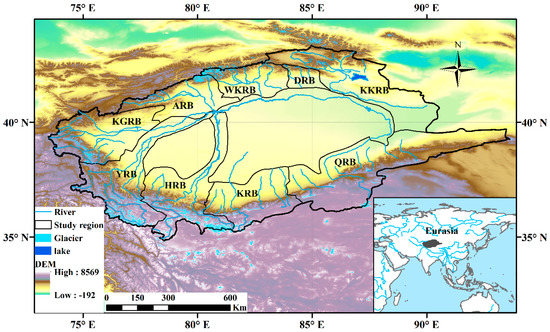
Figure 1.
Location of study region on the Tarim River Basin, including the headwaters of the Yarkand (YRB), Kaxgar (KGRB), Aksu (ARB), Hotan (HRB), Weigan-Kuqa (WKRB), Dina (DRB), Keriya (KRB), Kaidu-Kongque (KKRB), and Qarqan (QRB) River Basin; and glaciers, lakes, and elevations. DEM = digital elevation model.
2.2. Data
2.2.1. Meteorological Data
Precipitation (P) is deemed some of the most important data in the TRB’s water cycle [69]. Due to the harsh climatic and environmental conditions, there are few meteorological stations in the TRB. Thus, this research adopts four published global high-resolution precipitation datasets, namely (1) Asian Precipitation-Highly-Resolved Observational Data Integration Towards Evaluation (APHRODITE V1101 and V1101EX_R1) [70]; (2) The monthly 0.5° grid data of precipitation series generated by the Climatic Research Unit from the University of East Anglia in conjunction with the Hadley Centre (at the UK Met Office) [71]; (3) Princeton University and University of Southampton Hydro-climatology Group Bias Corrected Meteorological Forcing Dataset Versions 3 (PUSHGBC); and (4) Global Precipitation Climatology Centre (GPCC). All of these products can be used to offer accurate estimates of precipitation in the TRB.
On the other hand, Evapotranspiration (ET) is one of the most difficult hydrological variables to obtain [72], especially in a region with sparse long-term hydrological data like the TRB. So in this study, five types of ET products are proposed, including two land surface models (Global Land Data Assimilation System, version 1 and 2 (hereafter, GLDAS-1 and GLDAS-2)). The five products are: (1) GLDAS1-CLM; (2) GLDAS1-Mosaic; (3) GLDAS1-Noah; (4) GLDAS1-VIC; and (5) GLDAS2-Noah. Bear in mind that ET is also an essential variable and proposed as an input factor to reconstruct TWSA based on the LSTM model in this study.
Apart from P and ET, we also considered the influence of SM and temperature on TWSA when building our LSTM model. Mean monthly temperature readings from CRU and GLDAS-2 are also adopted due to temperature that may indirectly affect evaporation from the soil. Moreover, it has been revealed by numerous studies that a strong correlation appears between SM with GRACE-derived TWSA [39,58,73]. Further, it was illustrated that SM from GLDAS-2 has the best performance [58]. Consequently, we select the monthly SM data (kg/m2) from GLDAS-2 (0.25° × 0.25°) as an input factor to simulate TWSA based on the LSTM model.
2.2.2. GRACE Data
In this study, we selected two different GRACE data to estimate the changes in terrestrial water storage. The first source is Jet Propulsion Laboratory (JPL) GRACE RL05 mascon products (https://grace.jpl.nasa.gov/data/get-data/jpl_global_mascons/ (accessed on 1 January 2021)), and the other is GRACE RL05 Center for Space Research (CSR) mascon products [74], retrieved from the GRACE Tellus website of the University of Texas (http://www2.csr.utexas.edu/grace/RL05_mascons.html (accessed on 1 January 2021)). The subtle difference between the product of TWSA from JPL and CSR is mostly caused by the methods and parameters [75]. Based on Long’s method, seventeen months of missing data were interpolated [33]. The datasets used for additional information are presented (Table 2).
Table 2.
Brief Description of Datasets Used.
2.3. Methods
2.3.1. TWS Calculations
In this study, the JPL and CSR GRACE products were analyzed using the GRACE RL05 mascon solutions method. The two GRACE mascon datasets showed good performance at the basin scale. However, as the original GRACE data may be noisy because of the influences of atmospheric changes, some corrections and adjustments should be made when evaluating TWSA. The correction of a glacial isostatic adjustment was used to remove glacial rebound effects in a 3-D finite-element model [76]. The replacement of Earth’s oblateness scale (C20) coefficient was also done because C20 values have larger uncertainty [77]. For this, the degree-1 coefficients were calculated by using the Swenson method [78].
According to Equation (1), the terrestrial water storage changes (TWSCs) are computed using TWSA from the GRACE data in the TRB. The TWSCs for each month should be evaluated by the two different time derivatives of TWSA [79]. The changes in terrestrial water storage can be calculated as follows [80]:
where denotes TWSC for month t. Note that TWS is estimated as the average of two different TWSA products from JPL and CSR, such that TWS (t + 1) and TWS (t − 1) are terrestrial water storage for month t + 1 and t − 1, respectively. The time Δt is considered as 1 month to maintain consistency with the estimation of terrestrial water storage.
2.3.2. Design and Architecture of LSTM Deep Learning Models
We used deep learning-based models (i.e., LSTM, Figure 2) to reconstruct the TWSA data at set time scales under the Python software in this study. Long short-term memory network, the most advanced deep learning model, is a special kind of RNN. LSTM models are designed to overcome the weaknesses of conventional RNNs with regard to learning long-term dependencies. This model consists of three sections: an input layer, a few hidden layers, and an output layer. The LSTM not only provides input data but also remembers the states of the hidden neurons of the previous time steps. We set up four hidden layers, the number of neurons in each layer is 50, 50, 60, and 10, respectively. The optimizer that we used the LSTM model is Adam. The Time Step is 5 and the Batch Size is 10. As well, these models simplify solving the autocorrelation and the temporal lag of the data and avoid vanishing gradients [81]. The LSTM layer plays an important role in learning the time series data and maintaining previous information. At the same time, the fully connected layer on the top of the LSTM layer improves the fitting and learning ability of the model. Hence, the LSTM can serve as an alternative for reconstructing TWSA in places where long-time series hydrogeological data are difficult to get and complex hydrogeological characteristics.
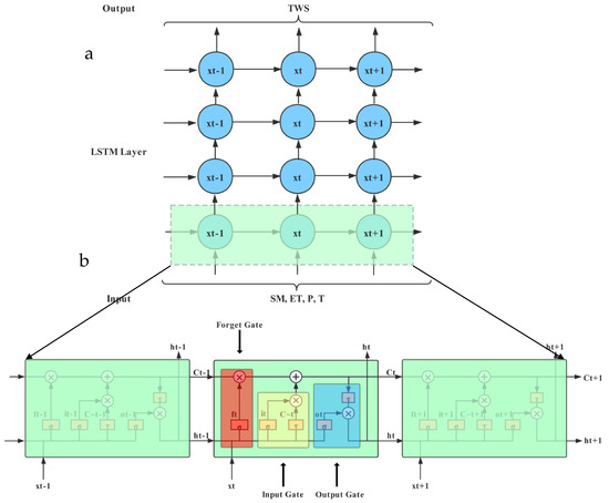
Figure 2.
(a) Chain-like structure of the Long Short-Term Memory (LSTM). (b) A graphical representation of LSTM’s memory block.
Various LSTM models have been used for flood forecasting, water table depth prediction, and water resources management [60,65]. A special multilayer recurrent neural network method [81], which is one of the most widely used LSTMs, is used jointly with the activation function of relu to reconstruct TWSA during the period 1982–2016. The multiple datasets of the four variables (P, ET, SM, and T) and TWSA unified the temporal resolution and spatial resolution. The multiple datasets of each variable are averaged and then put into the LSTM model for training. The input variables are P, ET, SM, and T, while the output data are the TWSA. Since the reconstruction of the data (1982–2003) is backward reconstruction, the time period of the model needs to be backward. For the LSTM model, GRACE-derived TWSA data covering 120 months (December 2012 to January 2003) are divided into three periods of the training (December 2012 to January 2006, 70% of all samples), validation (December 2005 to July 2004, 15% of all samples), and testing (June 2004 to January 2003, 15% of all samples). The training of the LSTM model is one of the nonlinear optimization problems, the purpose of which is to minimize the difference between the simulated results of the output layer and the observed results [21]. In this study, the activation function of relu is applied to train the network, as it requires less time in the convergence process. What is noteworthy is that multiple training will produce different results. Thus, in this process, statistical indicators (r and NRMSE) are used to select the suitable optimal network which is then used to reconstruct the TWSA during the period 1982–2002 in the TRB. The workflow exhibiting the reconstruction of TWSA based on the LSTM model across the TRB is shown in Figure 3.
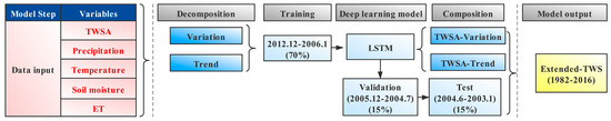
Figure 3.
The workflow of reconstruction the changes of terrestrial water storage.
2.3.3. Performance Metrics
In this study, evaluation criteria including Correlation Coefficient (r), Normalized Root-Mean-Square Error (NRMSE), Nash–Sutcliffe efficiency (NSE) coefficient [82], and relative bias (BIAS) are chosen to evaluate the simulated performance of the LSTM model. These criteria are calculated as follows:
where represents the estimated monthly values; denotes the observed monthly values; N indicates the number of months used for testing; and and are the mean values of and , respectively.
3. Results
3.1. Evaluation of GRACE TWSCs and Their Spatiotemporal Variability
The observations of GRACE can provide the monthly mean TWSA on a global scale. Figure 4 shows the monthly TWSA from JPL and CSR during the period 2002–2017. Results showed a significant correlation between the TWSA derived from JPL and CSR, with a correlation coefficient of 0.83. Additionally, it can reach a maximum and a minimum almost simultaneously. The uncertainty of TWSA can be computed from JPL (https://grace.jpl.nasa.gov/data/get-data/jpl_global_mascons.html (accessed on 1 January 2021)), and the uncertainty of CSR-derived TWSA can be determined using an uncertainty value of 2 cm equivalent water thickness (http://www2.csr.utexas.edu/grace/RL05_mascons.html (accessed on 1 January 2021)).
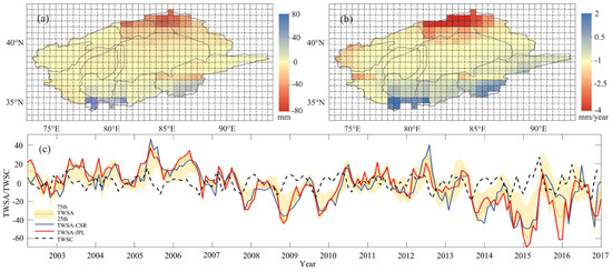
Figure 4.
The spatial–temporal distribution of Gravity Recovery and Climate Experiment (GRACE) terrestrial water storage anomalies (TWSA) derived from Jet Propulsion Laboratory (JPL) and Center for Space Research (CSR) during the period 2002–2017. ((a): spatial distribution of TWSA; (b): changing rate of TWSA; (c): temporal changes of average TWSA(mm) and TWSC(mm/month)).
The mean monthly TWSA is computed as the average of JPL-derived TWSA and CSR-derived TWSA with the view of diminishing the noise of equivalent water height. From Figure 4, the range for the mean monthly TWSA is between −59.47 and 41.47 mm in the TRB (relative to the baseline period from January 2004 to December 2009). Specifically, it shows a distinct seasonal cycle. The minimum and maximum values of TWSA were found in the winter (December to February) and summer (June to August). The monthly average water storage in the region was −4.53 mm, with the highest value in June 2005 (41.47 mm) and the lowest value in February 2015 (−59.47 mm). From 2002 to 2017, TWSA showed a significant downward trend (p < 0.001), with an average decline rate of 0.20 mm/month. Moreover, according to Equation (1), TWSC can be obtained from GRACE-derived TWSA in the study area. Then, the error can be calculated for the monthly TWSA to be approximately 9.6 mm, which is attributable to the measurement errors from 2002 to 2017 in the TRB. Figure 5 displays the spatial distribution of the TWSA from April 2002 to January 2017, averaged for different seasons. The TWSA shows obvious seasonal differences from spring to winter. It also reveals that the TWSA declined over a decade in the Tienshan Mountains, highlighting the phenomenon of the sum of TWSA in the north of the basin being less than that in the south of the basin from 2002 to 2017. Thus further, we found that the TWSA in spring declined significantly after 2014 (Figure 5e). It is believed that the decline in TWSA during the spring-time led to the decline of TWSA across the entire region. It is worth mentioning that this decline in spring-time terrestrial water storage may be related to the decrease in snow and glaciers cover in the Tienshan Mountains.
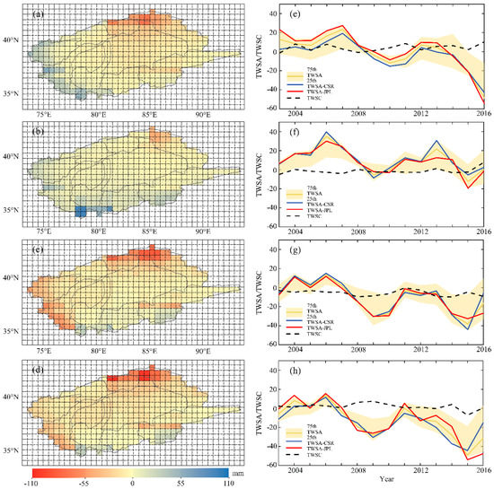
Figure 5.
The spatial–temporal distribution of the mean TWSA(mm) in different seasons from April 2002 to January 2017, (a,e) Spring (March–May), (b,f) Summer (June–August), (c,g) Autumn (September–November), and (d,h) Winter (December–February) in the Tarim River basin (TRB).
3.2. Estimation of Long-Term Time Series of Meteorological Data and Their Uncertainties
Figure 6a presents the seasonal cycles of four precipitation datasets (APHRODITE, PUSHGBC, CRU, and GPCC) was selected for the TRB., Findings disclosed that the precipitation from PUSHGBC is higher than that from the other three datasets, especially for the summertime, while the precipitation from APHRODITE is the lowest. The uncertainty of the overall average precipitation ranges from 0.49 to 32.68 mm/month, with the highest value observed in summer (40.21 mm) and the lowest in winter (0.22 mm). Note that the uncertainty of precipitation in 2016 cannot be obtained due to the lack of APHRODITE data. However, we assume that the average monthly precipitation in the region was 7.99 mm and the changes in precipitation from 1982 to 2016 were relatively stable. Despite the slight increase, the changing trend was not significant (p = 0.32), and the highest increase rate was detected in the upper reaches of the Tienshan Mountains.
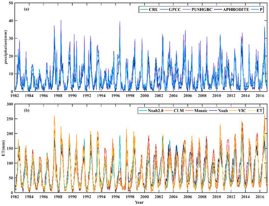
Figure 6.
(a) Comparisons of the four precipitation datasets from APHRODITE, PUSHGBC, CRU and GPCC during the period 1982–2016 in the TRB. (b) As in (a) but for five evapotranspiration (ET) datasets.
For large regions, it is difficult to obtain the actual ET at the in-situ measurements site, especially like the TRB, which has limited hydrological and meteorological data. For that, this study adopted five types of ET datasets to overcome these shortcomings. Therefore, Figure 6b shows the monthly ET rates, ranging from 5.99 to 211.11 mm following seasonal changes. In an overall perception, the ET increased from January to June, but decreased rapidly till December. The monthly average ET in the region was 69.59 mm. From 1982 to 2016, evapotranspiration showed a significant increasing trend (p < 0.005), and the average rate of change was 0.03 mm/month. The uncertainty of the monthly ET was calculated, ranging from approximately 0.47 to 263.04 mm. It is noteworthy that the value of ET in 1987 is abnormal, which may be the result of the difference between the five ET products. Nonetheless, these have a slight effect on the estimation of TWSA for the whole study period.
The climate of the TRB is predominantly temperate continental. Precipitation in the TRB shows clear seasonal variations (Figure 7a). The summer (June to August) accounts for about 50–70% of the annual total precipitation. Moreover, as displayed by Figure 7b, there is a good correspondence between the precipitation and the average ET, while Figure 7c demonstrates that the maximum TWSA occurred in July, which is consistent with the precipitation exhibited in Figure 7a. The nature of these findings unveils that the reduction in precipitation over different seasons will lead to the modifications in TWSA correspondingly. Consequently, climate change has not only affected the variations in precipitation and ET but also the variations in TWSA.
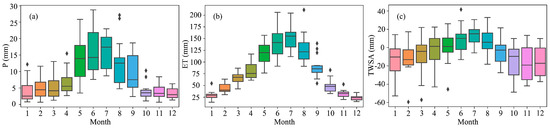
Figure 7.
The mean monthly (a) P, (b) ET, and (c) TWSA during the period 2003–2016 in the TRB.
3.3. Terrestrial Water Storage Anomalies Simulated from LSTM Models
The time scale of the GRACE data limits further estimations of terrestrial total water storage in the TRB. So, an LSTM model is used to establish the relationship between TWSA and hydrological data (P, ET, T, and SM) from 2003 to 2012 and accordingly apply it to reconstruct TWSA before 2003. Related researches indicated that SM has a significant correlation with TWSA. Thereby, we selected SM as an essential predictor and combined hydrological data. Additionally, we realized that the dataset of GLDAS-2 gives the best performance (r = 0.65) from 2003 to 2012, as shown in Figure 8.
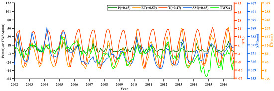
Figure 8.
Correlations between precipitation (P), ET, temperature (T), and soil moisture (SM) with TWSA. The results in parentheses represent the correlation coefficients between hydrological data with TWSA from 2003 to 2012.
To evaluate the effectiveness of the LSTM model, two performance metrics were selected, namely correlation coefficient and NRMSE. The LSTM model is proved to have satisfactory performance once the correlation coefficient is closer to 1 and a lower NRMSE value. Thereby, All of the LSTM predictors with their performances are presented, hence the comparison of the TWSA generated from GRACE and the LSTM model in different stages (Table 3).
Table 3.
Comparison Between LSTM-Generated TWSA and GRACE-Generated TWSA (2003–2012).
Taking note that the bolded value represents the best combination with 70%, 15%, 15%, and 100% representing the corresponding proportions to all samples in different periods.
From Table 3, the optimal combination of predictors is SM, ET, P, and T, which can best capture the characteristics of TWSA compared with remained combinations. Thus, using SM, ET, P, and T as predictors during the period 2003–2012, we simulated TWSA for the TRB based on the LSTM model, then again reconstructed the TWSA values from 1982 to 2002. Figure 9 displays the comparison of TWSA developed from both LSTM and GRACE. As can be depicted, TWSA generated by LSTM agrees well with GRACE’s one from 2003 to 2012, with a correlation efficient (r) of 0.922 and an NRMSE of 0.107, respectively. This indicates that the LSTM model indeed performs well in simulating time series data. Meanwhile TWSA exhibits an obvious seasonal cycle from 1982 to 2002. The monthly average water storage in the region is −1.60 mm, with the highest value in June 2005 (41.47 mm) and the lowest value in February 2015 (-59.47 mm). From 1982 to 2016, water storage unveiled a downward trend (p < 0.001), with an average decline rate of 0.03 mm/month. These data indicate that variables of SM, ET, P, and T in the LSTM model not only offer the simulation of TWSA, but also reconstruct the TWSA with a long-term time scale.
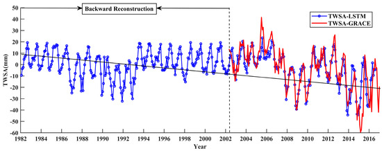
Figure 9.
Comparisons between the mean monthly TWSA from GRACE and LSTM-generated TWSA.
4. Discussion
Deep learning methods have been proven to be very helpful in solving some traditionally difficult problems (e.g., data reconstruction) [51]. In our study, TWSA generated by both LSTM and GRACE agrees well with each other’s from 2003 to 2012, with a high correlation efficient (r) of 0.922 and an NRMSE of 0.107, respectively. Likewise, Yang et al. [40] used the LSTM model to simulate the GHMs-based flood, and found the correlation coefficients to be 0.95, 0.98, and 0.99. These results indicated that the LSTM model presents a good performance in simulating time series data. Similarly, Sun et al. [21] reconstructed GRACE data by combining the CNN model and hydrological models. Generally, deep-learning techniques (e.g., LSTM model, CNN model) will promote the development of hydrology and related fields in the future [48,49,50]. Furthermore, in terms of predictor selection, we selected SM as an essential predictor and combined hydrological data, consistent with related researches that also mentioned SM to have a significant correlation with TWSA [80]. The Tarim River basin’s climate is predominantly temperate continental, which is the most common inland drought system in the world [71]. Figure 5 illustrates that the TWSA declined over a decade in the Tienshan Mountains, highlighting the phenomenon of the sum of TWSA in the north of the basin is less than that in the south of the basin from 2002 to 2017. Yang et al. [11] also reported the same phenomenon, but for a slightly shorter period (2002 to 2015). Furthermore, we realized that TWSA exhibited a significant downward trend (p < 0.001), with an average decline rate of 0.20 mm/month from 2002 to 2017. Similar findings were produced by Zhao and Li, [67] who found the TWS to slightly decrease with a declining trend of −1.4069 ± 0.5060 mm yr−1 in the TRB from 2002 to 2015. However, the reduction rate is slightly different due to the distinction in the selected timescale.
In general, the amplitudes of TWSA with the LSTM model are slightly higher than the TWSA from GRACE for the 1982–2016 period. However, this overestimation is reasonable when considering the groundwater storage changes [22]. This overestimation may come from the inherent uncertainty of TWSA. Even though the LSTM model provides an effective method for estimating TWSA, it still poses some uncertainties and errors. The uncertainty of the reconstructed TWSA could be attributed to two reasons: the uncertainty of the reanalysis datasets and the uncertainty of the LSTM model. Primarily, due to limited training sample data in this study, the results may be affected [22]. Moreover, there is a range of uncertainty in P and ET, which may result in either underestimation or overestimation of TWSA due to the complex geographical conditions in TRB’s areas (Figure 6). Secondly, the LSTM model provides a mathematically effective, pattern recognition technique that can generate complex algorithms describing the relationships among several input and output variables, and the model can be used to deal with the non-linear and seasonal tendencies data. Generally, the LSTM model cannot explain the physical dynamics in TWS since it is a relative “black box” compared with the logistic regression model [81]. This may reduce the confidence of the LSTM models. At the same time, this forecast result produced by the LSTM model may have some fluctuations, which is also quite normal [58]. The short-term prediction effect of this model is better, and the long-term trend volatility is indeed a bit large. Moreover, the determination of the appropriate LSTM model structure is another factor that affects the accuracy of the model, which calls for more and in-depth calibration of the model structure. In the current study, the best structure model was selected among seven combinations (Table 3) by comparing the errors between results and observations. More LSTM models with different architectures applied for evaluating results will improve the accuracy and reduce the uncertainty. Notwithstanding the goodness of LSTM in timing simulations, it still has obvious shortcomings when applied in spatial simulations.
In addition, some human-mediated activities such as irrigation and extraction of groundwater among others can also lead to water imbalance for regions [22]. For instance, some studies proved that irrigation affects the actual runoff and ET in the Aksu and Yarkand River basins [12]. Additionally, it is well known that the two main streams (Aksu River and Yarkand River) comprise the main agricultural regions in TRB. For future work, more efforts will be invested into various components of TWS, such as surface water and groundwater. In addition, a combination of CMIP6 data and an LSTM model will be drawn to simulate future water storage changes. Lately, this study mainly compares the TWSA trend of the LSTM model and GRACE dataset to complement the previous researches on fluxes (e.g., river discharge, ET). Yet, future investigations should take into account the hydrological process with physical mechanism models for verification. Thus, we relied on this model since it is the first attempt to be undertaken over the study area of interest, and its accuracy will be strengthened in the follow-up investigations.
5. Conclusions
The GRACE dataset provides an unprecedented opportunity for studying TWS, including changes in surface storage and groundwater storage. From 2002 to 2017, TWSA showed a significant downward trend (p < 0.001), with an average decline rate of 0.20 mm/month in the TRB. However, in this study, our goal was to generate a convenient and effective method for reconstructing total TWSA. The LSTM model using SM, P, T, and ET as predictors was used to generate a longer monthly TWSA. The modeled findings showed that the LSTM-generated TWSA was largely consistent with GRACE, with a correlation efficient (r) of 0.922 and an NRMSE of 0.107 (SM, ET, P, and T) during the period 2003–2012. This finding demonstrated that using the LSTM model can be an effective approach to generate TWSA. Furthermore, the structure of the model proved to be logical, and the LSTM helped to prevent overfitting effectively. Finally, TWSA showed a downward trend (p < 0.001), with an average decline rate of 0.03 mm/month in the TRB in the period 1982–2016.
Author Contributions
Conceptualization, Y.C. and F.W.; methodology, F.W.; validation, F.W. and X.W.; investigation, F.W.; data curation, F.W.; writing—original draft preparation, F.W.; writing—review and editing, Y.C., Z.L., G.F., Y.L., X.W., X.Z. and P.M.K.; project administration, Y.C.; funding acquisition, Y.C. All authors have read and agreed to the published version of the manuscript.
Funding
This research was funded by the Strategic Priority Research Program of Chinese Academy of Sciences, (Grant No. XDA20100303) and the Key Research Program of the Chinese Academy of Sciences (ZDRWZS–2019–3).
Acknowledgments
We appreciate the editors and the reviewers for their constructive suggestions and insightful comments, which helped us greatly to improve this manuscript.
Conflicts of Interest
The authors declare no conflict of interest.
References
- Deng, H.; Chen, Y. Influences of recent climate change and human activities on water storage variations in Central Asia. J. Hydrol. 2017, 544, 46–57. [Google Scholar] [CrossRef]
- Pellet, V.; Aires, F.; Papa, F.; Munier, S.; Decharme, B. Long-term Total Water Storage Change from a SAtellite Water Cycle (SAWC) reconstruction over large south Asian basins. Hydrol. Earth Syst. Sci. Discuss. 2019, 1–30. [Google Scholar] [CrossRef]
- Zhao, M.; Geruo, A.; Zhang, J.; Velicogna, I.; Liang, C.; Li, Z. Ecological restoration impact on total terrestrial water storage. Nat. Sustain. 2021, 4, 56–62. [Google Scholar] [CrossRef]
- Famiglietti, J.S. Remote sensing of terrestrial water storage, soil moisture and surface waters. Wash. Dc Am. Geophys. Union Geophys. Monogr. Ser. 2004, 150, 197–207. [Google Scholar]
- Wang, J.; Song, C.; Reager, J.T.; Yao, F.; Famiglietti, J.S.; Sheng, Y.; MacDonald, G.M.; Brun, F.; Schmied, H.M.; Marston, R.A. Recent global decline in endorheic basin water storages. Nat. Geosci. 2018, 11, 926–932. [Google Scholar] [CrossRef]
- Scanlon, B.R.; Zhang, Z.; Save, H.; Sun, A.Y.; Schmied, H.M.; Van Beek, L.P.; Wiese, D.N.; Wada, Y.; Long, D.; Reedy, R.C. Global models underestimate large decadal declining and rising water storage trends relative to GRACE satellite data. Proc. Natl. Acad. Sci. USA 2018, 115, 1080–1089. [Google Scholar] [CrossRef] [PubMed]
- Xie, J.; Xu, Y.-P.; Wang, Y.; Gu, H.; Wang, F.; Pan, S. Influences of climatic variability and human activities on terrestrial water storage variations across the Yellow River basin in the recent decade. J. Hydrol. 2019, 579, 124218. [Google Scholar] [CrossRef]
- Xie, Y.; Huang, S.; Liu, S.; Leng, G.; Peng, J.; Huang, Q.; Li, P. GRACE-based terrestrial water storage in Northwest China: Changes and causes. Remote Sens. 2018, 10, 1163. [Google Scholar] [CrossRef]
- Yang, P.; Xia, J.; Zhan, C.; Wang, T. Reconstruction of terrestrial water storage anomalies in Northwest China during 1948–2002 using GRACE and GLDAS products. Hydrol. Res. 2018, 49, 1594–1607. [Google Scholar] [CrossRef]
- Chen, Y.; Li, Z.; Li, W.; Deng, H.; Shen, Y. Water and ecological security: Dealing with hydroclimatic challenges at the heart of China’s Silk Road. Environ. Earth Sci. 2016, 75, 881. [Google Scholar] [CrossRef]
- Yang, P.; Xia, J.; Zhan, C.; Qiao, Y.; Wang, Y. Monitoring the spatio-temporal changes of terrestrial water storage using GRACE data in the Tarim River basin between 2002 and 2015. Sci. Total Environ. 2017, 595, 218–228. [Google Scholar] [CrossRef]
- Wang, F.; Chen, Y.; Li, Z.; Fang, G.; Li, Y.; Xia, Z. Assessment of the Irrigation Water Requirement and Water Supply Risk in the Tarim River Basin, Northwest China. Sustainability 2019, 11, 4941. [Google Scholar] [CrossRef]
- Rodell, M.; Famiglietti, J.; Wiese, D.; Reager, J.; Beaudoing, H.; Landerer, F.W.; Lo, M.-H. Emerging trends in global freshwater availability. Nature 2018, 557, 651–659. [Google Scholar] [CrossRef] [PubMed]
- Richey, A.S.; Thomas, B.F.; Lo, M.H.; Reager, J.T.; Famiglietti, J.S.; Voss, K.; Swenson, S.; Rodell, M. Quantifying renewable groundwater stress with GRACE. Water Resour. Res. 2015, 51, 5217–5238. [Google Scholar] [CrossRef]
- Wada, Y.; Van Beek, L.P.; Wanders, N.; Bierkens, M.F. Human water consumption intensifies hydrological drought worldwide. Environ. Res. Lett. 2013, 8, 034036. [Google Scholar] [CrossRef]
- Wang, X.; Xiao, X.; Zou, Z.; Dong, J.; Qin, Y.; Doughty, R.B.; Menarguez, M.A.; Chen, B.; Wang, J.; Ye, H.; et al. Gainers and losers of surface and terrestrial water resources in China during 1989–2016. Nat. Commun. 2020, 11, 3471. [Google Scholar] [CrossRef]
- Eom, J.; Seo, K.-W.; Ryu, D. Estimation of Amazon River discharge based on EOF analysis of GRACE gravity data. Remote Sens. Environ. 2017, 191, 55–66. [Google Scholar] [CrossRef]
- Yang, T.; Wang, C.; Chen, Y.; Chen, X.; Yu, Z. Climate change and water storage variability over an arid endorheic region. J. Hydrol. 2015, 529, 330–339. [Google Scholar] [CrossRef]
- Castellazzi, P.; Martel, R.; Rivera, A.; Huang, J.; Pavlic, G.; Calderhead, A.I.; Chaussard, E.; Garfias, J.; Salas, J. Groundwater depletion in Central Mexico: Use of GRACE and InSAR to support water resources management. Water Resour. Res. 2016, 52, 5985–6003. [Google Scholar] [CrossRef]
- Tian, S.; Tregoning, P.; Renzullo, L.J.; van Dijk, A.I.; Walker, J.P.; Pauwels, V.R.; Allgeyer, S. Improved water balance component estimates through joint assimilation of GRACE water storage and SMOS soil moisture retrievals. Water Resour. Res. 2017, 53, 1820–1840. [Google Scholar] [CrossRef]
- Sun, A.Y.; Scanlon, B.R.; Zhang, Z.; Walling, D.; Bhanja, S.N.; Mukherjee, A.; Zhong, Z. Combining Physically Based Modeling and Deep Learning for Fusing GRACE Satellite Data: Can We Learn From Mismatch? Water Resour. Res. 2019, 55, 1179–1195. [Google Scholar] [CrossRef]
- Zhang, J.; Zhu, Y.; Zhang, X.; Ye, M.; Yang, J. Developing a Long Short-Term Memory (LSTM) based model for predicting water table depth in agricultural areas. J. Hydrol. 2018, 561, 918–929. [Google Scholar] [CrossRef]
- Feng, W.; Zhong, M.; Lemoine, J.M.; Biancale, R.; Hsu, H.T.; Xia, J. Evaluation of groundwater depletion in North China using the Gravity Recovery and Climate Experiment (GRACE) data and ground-based measurements. Water Resour. Res. 2013, 49, 2110–2118. [Google Scholar] [CrossRef]
- Tangdamrongsub, N.; Han, S.-C.; Yeo, I.-Y.; Dong, J.; Steele-Dunne, S.C.; Willgoose, G.; Walker, J.P. Multivariate data assimilation of GRACE, SMOS, SMAP measurements for improved regional soil moisture and groundwater storage estimates. Adv. Water Resour. 2020, 135, 103477. [Google Scholar] [CrossRef]
- Chen, L.; He, Q.; Liu, K.; Li, J.; Jing, C. Downscaling of GRACE-Derived Groundwater Storage Based on the Random Forest Model. Remote Sens. 2019, 11, 2979. [Google Scholar] [CrossRef]
- Long, D.; Yang, W.; Scanlon, B.R.; Zhao, J.; Liu, D.; Burek, P.; Pan, Y.; You, L.; Wada, Y. South-to-North Water Diversion stabilizing Beijing’s groundwater levels. Nat. Commun. 2020, 11, 3665. [Google Scholar] [CrossRef]
- Yin, W.; Hu, L.; Zheng, W.; Jiao, J.J.; Han, S.-C.; Zhang, M. Assessing underground water-exchange between regions using GRACE data. J. Geophys. Res. Atmos. 2020, 125, e2020JD032570. [Google Scholar] [CrossRef]
- Zhang, H.; Zhang, L.L.; Li, J.; An, R.D.; Deng, Y. Monitoring the spatiotemporal terrestrial water storage changes in the Yarlung Zangbo River Basin by applying the P-LSA and EOF methods to GRACE data. Sci. Total Environ. 2020, 713, 136274. [Google Scholar] [CrossRef]
- Jing, W.; Yao, L.; Zhao, X.; Zhang, P.; Liu, Y.; Xia, X.; Song, J.; Yang, J.; Li, Y.; Zhou, C. Understanding terrestrial water storage declining trends in the Yellow River Basin. J. Geophys. Res. Atmos. 2019, 124, 12963–12984. [Google Scholar] [CrossRef]
- Seyoum, W.M.; Milewski, A.M. Monitoring and comparison of terrestrial water storage changes in the northern high plains using GRACE and in-situ based integrated hydrologic model estimates. Adv. Water Resour. 2016, 94, 31–44. [Google Scholar] [CrossRef]
- Deng, H.; Pepin, N.; Liu, Q.; Chen, Y. Understanding the spatial differences in terrestrial water storage variations in the Tibetan Plateau from 2002 to 2016. Clim. Chang. 2018, 151, 379–393. [Google Scholar] [CrossRef]
- Deng, H.; Chen, Y.; Li, Q.; Lin, G. Loss of terrestrial water storage in the Tianshan mountains from 2003 to 2015. Int. J. Remote Sens. 2019, 40, 8342–8358. [Google Scholar] [CrossRef]
- Long, D.; Yang, Y.; Wada, Y.; Hong, Y.; Liang, W.; Chen, Y.; Yong, B.; Hou, A.; Wei, J.; Chen, L. Deriving scaling factors using a global hydrological model to restore GRACE total water storage changes for China’s Yangtze River Basin. Remote Sens. Environ. 2015, 168, 177–193. [Google Scholar] [CrossRef]
- Gerdener, H.; Engels, O.; Kusche, J. A framework for deriving drought indicators from the Gravity Recovery and Climate Experiment (GRACE). Hydrol. Earth Syst. Sci. 2020, 24, 227–248. [Google Scholar] [CrossRef]
- Liu, X.; Feng, X.; Ciais, P.; Fu, B.; Hu, B.; Sun, Z. GRACE satellite-based drought index indicating increased impact of drought over major basins in China during 2002–2017. Agric. For. Meteorol. 2020, 291, 108057. [Google Scholar] [CrossRef]
- Sun, Z.; Zhu, X.; Pan, Y.; Zhang, J.; Liu, X. Drought evaluation using the GRACE terrestrial water storage deficit over the Yangtze River Basin, China. Sci. Total Environ. 2018, 634, 727–738. [Google Scholar] [CrossRef]
- Xia, J.; Yang, P.; Zhan, C.; Qiao, Y. Analysis of changes in drought and terrestrial water storage in the Tarim River Basin based on principal component analysis. Hydrol. Res. 2019, 50, 761–777. [Google Scholar] [CrossRef]
- Chen, J.L.; Wilson, C.R.; Tapley, B.D. The 2009 exceptional Amazon flood and interannual terrestrial water storage change observed by GRACE. Water Resour. Res. 2010, 46. [Google Scholar] [CrossRef]
- Long, D.; Shen, Y.; Sun, A.; Hong, Y.; Longuevergne, L.; Yang, Y.; Li, B.; Chen, L. Drought and flood monitoring for a large karst plateau in Southwest China using extended GRACE data. Remote Sens. Environ. 2014, 155, 145–160. [Google Scholar] [CrossRef]
- Yang, T.; Sun, F.; Gentine, P.; Liu, W.; Wang, H.; Yin, J.; Du, M.; Liu, C. Evaluation and machine learning improvement of global hydrological model-based flood simulations. Environ. Res. Lett. 2019, 14, 114027. [Google Scholar] [CrossRef]
- Loomis, B.D.; Rachlin, K.E.; Wiese, D.N.; Landerer, F.W.; Luthcke, S.B. Replacing GRACE/GRACE-FO C30 with satellite laser ranging: Impacts on Antarctic Ice Sheet mass change. Geophys. Res. Lett. 2020, e2019GL085488. [Google Scholar]
- Famiglietti, J.S.; Rodell, M. Water in the balance. Science 2013, 340, 1300–1301. [Google Scholar] [CrossRef]
- Croteau, M.J.; Nerem, R.S.; Loomis, B.D.; Sabaka, T.J. Development of a Daily GRACE Mascon Solution for Terrestrial Water Storage. J. Geophys. Res. 2020, 125, e2019JB018468. [Google Scholar] [CrossRef]
- Yin, W.; Hu, L.; Han, S.-C.; Zhang, M.; Teng, Y. Reconstructing Terrestrial Water Storage Variations from 1980 to 2015 in the Beishan Area of China. Geofluids 2019, 2019. [Google Scholar] [CrossRef]
- Tang, Y.; Hooshyar, M.; Zhu, T.; Ringler, C.; Sun, A.Y.; Long, D.; Wang, D. Reconstructing annual groundwater storage changes in a large-scale irrigation region using GRACE data and Budyko model. J. Hydrol. 2017, 551, 397–406. [Google Scholar] [CrossRef]
- Hasan, E.; Tarhule, A.; Zume, J.T.; Kirstetter, P.-E. + 50 Years of Terrestrial Hydroclimatic Variability in Africa’s Transboundary Waters. Sci. Rep. 2019, 9, 1–12. [Google Scholar] [CrossRef] [PubMed]
- Hamshaw, S.D.; Dewoolkar, M.M.; Schroth, A.W.; Wemple, B.C.; Rizzo, D.M. A New Machine-Learning Approach for Classifying Hysteresis in Suspended-Sediment Discharge Relationships Using High-Frequency Monitoring Data. Water Resour. Res. 2018, 54, 4040–4058. [Google Scholar] [CrossRef]
- Sun, A.Y.; Scanlon, B.R. How can Big Data and machine learning benefit environment and water management: A survey of methods, applications, and future directions. Environ. Res. Lett. 2019, 14, 073001. [Google Scholar] [CrossRef]
- Reichstein, M.; Camps-Valls, G.; Stevens, B.; Jung, M.; Denzler, J.; Carvalhais, N. Deep learning and process understanding for data-driven Earth system science. Nature 2019, 566, 195–204. [Google Scholar] [CrossRef]
- Xue, M.; Hang, R.; Liu, Q.; Yuan, X.-T.; Lu, X. CNN-based near-real-time precipitation estimation from Fengyun-2 satellite over Xinjiang, China. Atmos. Res. 2021, 250, 105337. [Google Scholar] [CrossRef]
- Li, F.; Kusche, J.; Rietbroek, R.; Wang, Z.; Forootan, E.; Schulze, K.; Luck, C. Comparison of Data-driven Techniques to Reconstruct (1992–2002) and Predict (2017–2018) GRACE-like Gridded Total Water Storage Changes using Climate Inputs. Water Resour. Res. 2020, 56, e2019WR026551. [Google Scholar] [CrossRef]
- Broxton, P.D.; Van Leeuwen, W.J.D.; Biederman, J.A. Improving Snow Water Equivalent Maps With Machine Learning of Snow Survey and Lidar Measurements. Water Resour. Res. 2019, 55, 3739–3757. [Google Scholar] [CrossRef]
- Kim, D.; Yu, H.; Lee, H.; Beighley, E.; Durand, M.; Alsdorf, D.; Hwang, E. Ensemble learning regression for estimating river discharges using satellite altimetry data: Central Congo River as a Test-bed. Remote Sens. Environ. 2019, 221, 741–755. [Google Scholar] [CrossRef]
- Sahoo, S.; Russo, T.A.; Elliott, J.; Foster, I. Machine learning algorithms for modeling groundwater level changes in agricultural regions of the U.S. Water Resour. Res. 2017, 53, 3878–3895. [Google Scholar] [CrossRef]
- Jing, W.; Zhao, X.; Yao, L.; Di, L.; Yang, J.; Li, Y.; Guo, L.; Zhou, C. Can terrestrial water storage dynamics be estimated from climate anomalies. Earth Space Sci. 2020, 7, e2019EA000959. [Google Scholar] [CrossRef]
- Sun, Z.; Long, D.; Yang, W.; Li, X.; Pan, Y. Reconstruction of GRACE Data on Changes in Total Water Storage Over the Global Land Surface and 60 Basins. Water Resour. Res. 2020, 56, e2019WR026250. [Google Scholar] [CrossRef]
- Jing, W.; Zhang, P.; Zhao, X.; Yang, Y.; Jiang, H.; Xu, J.; Yang, J.; Li, Y. Extending GRACE terrestrial water storage anomalies by combining the random forest regression and a spatially moving window structure. J. Hydrol. 2020, 590, 125239. [Google Scholar] [CrossRef]
- Xie, J.; Xu, Y.P.; Gao, C.; Xuan, W.; Bai, Z. Total basin discharge from GRACE and Water balance method for the Yarlung Tsangpo River basin, Southwestern China. J. Geophys. Res. Atmos. 2019, 124, 7617–7632. [Google Scholar] [CrossRef]
- Le, X.H.; Ho, H.V.; Lee, G.; Jung, S. Application of Long Short-Term Memory (LSTM) Neural Network for Flood Forecasting. Water 2019, 11, 1387. [Google Scholar] [CrossRef]
- Asanjan, A.A.; Yang, T.; Hsu, K.; Sorooshian, S.; Lin, J.; Peng, Q. Short-Term Precipitation Forecast Based on the PERSIANN System and LSTM Recurrent Neural Networks. J. Geophys. Res. 2018, 123, 12–563. [Google Scholar]
- Tennant, C.; Larsen, L.; Bellugi, D.; Moges, E.; Zhang, L.; Ma, H. The utility of information flow in formulating discharge forecast models: A case study from an arid snow-dominated catchment. Water Resour. Res. 2020, 56, e2019WR024908. [Google Scholar] [CrossRef]
- Zhu, S.; Luo, X.; Yuan, X.; Xu, Z. An improved long short-term memory network for streamflow forecasting in the upper Yangtze River. Stoch. Environ. Res. Risk Assess. 2020, 34, 1313–1329. [Google Scholar] [CrossRef]
- Kratzert, F.; Klotz, D.; Brenner, C.; Schulz, K.; Herrnegger, M. Rainfall–runoff modelling using long short-term memory (LSTM) networks. Hydrol. Earth Syst. Sci. 2018, 22, 6005–6022. [Google Scholar] [CrossRef]
- Hu, C.; Wu, Q.; Li, H.; Jian, S.; Li, N.; Lou, Z. Deep Learning with a Long Short-Term Memory Networks Approach for Rainfall-Runoff Simulation. Water 2018, 10, 1543. [Google Scholar] [CrossRef]
- Sahoo, B.B.; Jha, R.; Singh, A.; Kumar, D. Long short-term memory (LSTM) recurrent neural network for low-flow hydrological time series forecasting. Acta Geophys. 2019, 67, 1471–1481. [Google Scholar] [CrossRef]
- Huang, X.; Gao, L.; Crosbie, R.S.; Zhang, N.; Fu, G.; Doble, R. Groundwater Recharge Prediction Using Linear Regression, Multi-Layer Perception Network, and Deep Learning. Water 2019, 11, 1879. [Google Scholar] [CrossRef]
- Zhao, K.; Li, X. Estimating terrestrial water storage changes in the Tarim River Basin using GRACE data. Geophys. J. Int. 2017, 211, 1449–1460. [Google Scholar] [CrossRef]
- Yang, P.; Xia, J.; Zhan, C.; Zhang, Y.; Chen, J. Study on the Variation of Terrestrial Water Storage and the Identification of Its Relationship with Hydrological Cycle Factors in the Tarim River Basin, China. Adv. Meteorol. 2017, 2017, 1–11. [Google Scholar] [CrossRef]
- Chen, X.; Long, D.; Hong, Y.; Zeng, C.; Yan, D. Improved modeling of snow and glacier melting by a progressive two-stage calibration strategy with GRACE and multisource data: How snow and glacier meltwater contributes to the runoff of the Upper Brahmaputra River basin? Water Resour. Res. 2017, 53, 2431–2466. [Google Scholar] [CrossRef]
- Dong, W.; Lin, Y.; Wright, J.S.; Xie, Y.; Ming, Y.; Zhang, H.; Chen, R.; Chen, Y.; Xu, F.; Lin, N. Regional disparities in warm season rainfall changes over arid eastern–central Asia. Sci. Rep. 2018, 8, 1–11. [Google Scholar]
- Li, Z.; Chen, Y.; Li, W.; Deng, H.; Fang, G. Potential impacts of climate change on vegetation dynamics in Central Asia. J. Geophys. Res. 2015, 120, 12345–12356. [Google Scholar] [CrossRef]
- Wang, H.; Guan, H.; Gutiérrez-Jurado, H.A.; Simmons, C.T. Examination of water budget using satellite products over Australia. J. Hydrol. 2014, 511, 546–554. [Google Scholar] [CrossRef]
- Meng, L.; Long, D.; Quiring, S.M.; Shen, Y. Statistical analysis of the relationship between spring soil moisture and summer precipitation in East China. Int. J. Climatol. 2014, 34, 1511–1523. [Google Scholar] [CrossRef]
- Save, H.; Bettadpur, S.; Tapley, B.D. High-resolution CSR GRACE RL05 mascons. J. Geophys. Res. 2016, 121, 7547–7569. [Google Scholar] [CrossRef]
- Scanlon, B.R.; Zhang, Z.; Save, H.; Wiese, D.N.; Landerer, F.W.; Long, D.; Longuevergne, L.; Chen, J. Global evaluation of new GRACE mascon products for hydrologic applications. Water Resour. Res. 2016, 52, 9412–9429. [Google Scholar] [CrossRef]
- Wahr, J.; Zhong, S. Computations of the viscoelastic response of a 3-D compressible Earth to surface loading: An application to Glacial Isostatic Adjustment in Antarctica and Canada. Geophys. J. Int. 2013, 192, 557–572. [Google Scholar]
- Cheng, M.; Ries, J.C.; Tapley, B.D. Variations of the Earth’s figure axis from satellite laser ranging and GRACE. J. Geophys. Res. Solid Earth 2015, 116. [Google Scholar] [CrossRef]
- Swenson, S.; Chambers, D.; Wahr, J. Estimating geocenter variations from a combination of GRACE and ocean model output. J. Geophys. Res. Solid Earth 2008, 113. [Google Scholar] [CrossRef]
- Ramillien, G.; Frappart, F.; Guntner, A.; Ngoduc, T.; Cazenave, A.; Laval, K. Time variations of the regional evapotranspiration rate from Gravity Recovery and Climate Experiment (GRACE) satellite gravimetry. Water Resour. Res. 2006, 42. [Google Scholar] [CrossRef]
- Long, D.; Longuevergne, L.; Scanlon, B.R. Uncertainty in evapotranspiration from land surface modeling, remote sensing, and GRACE satellites. Water Resour. Res. 2014, 50, 1131–1151. [Google Scholar] [CrossRef]
- Hochreiter, S.; Schmidhuber, J. Long short-term memory. Neural Comput. 1997, 9, 1735–1780. [Google Scholar] [CrossRef] [PubMed]
- Nash, J.E.; Sutcliffe, J.V. River flow forecasting through conceptual models part I—A discussion of principles. J. Hydrol. 1970, 10, 282–290. [Google Scholar] [CrossRef]


Publisher’s Note: MDPI stays neutral with regard to jurisdictional claims in published maps and institutional affiliations. |
© 2021 by the authors. Licensee MDPI, Basel, Switzerland. This article is an open access article distributed under the terms and conditions of the Creative Commons Attribution (CC BY) license (http://creativecommons.org/licenses/by/4.0/).