Subpixel Change Detection Based on Radial Basis Function with Abundance Image Difference Measure for Remote Sensing Images

Abstract

Recently, land cover change detection has become a research focus of remote sensing. To obtain the change information from remote sensing images at fine spatial and temporal resolutions, subpixel change detection is widely studied and applied. In this paper, a new subpixel change detection method based on radial basis function (RBF) for remote sensing images is proposed, in which the abundance image difference measure (AIDM) is designed and utilized to enhance the subpixel mapping (SPM) by borrowing the fine spatial distribution of the fine spatial resolution image to decrease the influence of the spectral unmixing error. First, the fine and coarse spatial resolution images are used to develop subpixel change detection. Second, linear spectral mixing modeling and the degradation procedure are conducted on the coarse and fine spatial resolution image to produce two temporal abundance images, respectively. Then, the designed AIDM is utilized to enhance the RBF-based SPM by comparing the two temporal abundance images. At last, the proposed RBF-AIDM method is applied for SPM and subpixel change detection. The synthetic images based on Landsat-7 Enhanced Thematic Mapper Plus (ETM+) and real case images based on two temporal Landsat-8 Operational Land Imager (OLI) images and one Moderate Resolution Imaging Spectroradiometer (MODIS) image are undertaken to validate the proposed method. The experimental results indicate that the proposed method can sufficiently decrease the influence of the spectral unmixing error and improve the subpixel change detection results.

1. Introduction

In remote sensing, change detection is the process that identifies the differences that have occurred on the Earth’s surface by observing multi-temporal images acquired in the same area at different times [1,2,3,4,5]. With the advancement of remote sensing technology, the acquisition of multi-temporal remote sensing images over a certain area is becoming more convenient. Under this background, it is possible to detect land cover changes using remote sensing change detection methods, and it has been one of the most important ways of land cover change detection. Remote sensing change detection methods have been successfully applied in many fields, such as environmental monitoring [6,7], agricultural surveys [8], urban studies [9,10] and forest monitoring [11,12]. At present, land cover change detection from remote sensing images has become a research focus in remote sensing.

Over the past few decades, a large variety of change detection methods using remote sensing images have been developed. Generally, remote sensing change detection methods consist of three steps, namely, pre-processing, difference image generation and change detection technique selection. (1) The pre-processing stage mainly includes geometry correction and radiative correction to address the problems caused by radiometric difference, atmospheric difference and geometrical location difference between bi-temporal remote sensing images. (2) The difference image generation stage is to create the difference image between bi-temporal remote sensing images, and common difference image generation methods include image difference [13], image ratio [14] and change vector analysis [15]. (3) The change detection technique selection stage is to generate the change map in terms of the difference image, and common change detection techniques include threshold-based methods [16,17], clustering-based methods [18,19], post-classification methods [20,21] machine learning-based methods [22,23]. Moreover, deep learning-based change detection techniques have been widely applied in remote sensing research [24,25]. The aforementioned methods have been proved to be effective by practice.

In recent years, the change rate of the Earth’s surface is accelerating with the development of technology and human behavior. Thus, the change detection results are required to be obtained at a fine spatial resolution for detecting sufficient details. At the same time, a fine temporal resolution is also required to detect changes in a short period, such as in disaster monitoring. However, the reality is that sensors with fine spatial resolution usually have a long revisit time, and sensors with fine temporal resolution always have a low spatial resolution in contrast. For example, remote sensing images acquired by Landsat sensors have 30 meters’ spatial resolution, but the revisit time is 16 days. Correspondingly, remote sensing images acquired by the Moderate Resolution Imaging Spectroradiometer (MODIS) sensors have 500 m spatial resolution, but the revisit time is 1 day. Hence, it is necessary to develop change detection techniques at both fine spatial and temporal resolutions.

To address the aforementioned problems, some researchers have started to pay attention to spectral unmixing and subpixel change detection methods. As we know, mixed pixels are a widespread phenomenon within remote sensing images, especially within coarse spatial resolution images. In a mixed pixel, it generally covers a large area and contains more than one type of land cover class. Obviously, the existence of mixed pixels plays an important role in restricting the accuracy of change detection at fine spatial and temporal resolution remote sensing images. Spectral unmixing, as a mixed pixel analysis technique, has been developed for decades to extract land cover information within mixed pixels and it has already been utilized in change detection [26,27]. Lu et al. [26] proposed the linear spectral mixture analysis of multi-temporal thematic mapper images to detect land-cover change in Rondônia, Brazilian Amazon basin. Yokoya et al. [27] presented a new multi-sensor coupled spectral unmixing framework, and the framework solved unmixing problems involving a set of multi-sensor time-series spectral images in order to understand the dynamic changes of the surface at a subpixel scale. However, we can only acquire the change information at the pixel level and cannot obtain detailed information about changes at a fine spatial resolution using spectral unmixing techniques simply for change detection. For this reason, change detection methods based on subpixel mapping (SPM) between remote sensing images with different spatial and temporal resolutions have been developed in recent years [28,29,30]. Wang et al. [28] proposed a new subpixel resolution land cover change detection method based on the Hopfield neural network. Wu et al. [29] presented a new approach based on a back-propagation neural network with a high resolution map, in which a supervised model was introduced into subpixel land-cover change detection. He et al. [30] proposed the joint spectral–spatial–temporal maximum a posteriori (MAP)-based model for subpixel change detection, in which a newly developed temporal regularization model was added to the MAP model.

Although efforts have been made to improve the change detection methods at fine spatial and temporal resolutions, practical and effective methods still need to be developed. In this paper, we focus on the subpixel change detection method to detect fine spatial and temporal resolution changes. In remote sensing, SPM can be considered the post-processing of spectral unmixing, and it is a technique to obtain a fine spatial resolution land cover map using abundance images by estimating their spatial contribution [31,32,33,34,35]. Subpixel change detection is a promising technique for its providing of fine spatial resolution thematic maps of land cover changes. Wang et al. [33] proposed a new SPM method based on radial basis function (RBF) interpolation, in which the subpixel soft class values were calculated by RBF interpolation. Based on RBF-based SPM, a subpixel change detection method was proposed to detect changes at fine spatial and temporal resolutions, and the experimental results showed the effectiveness of the proposed subpixel change detection method [36]. Although the RBF-based subpixel change detection method has been demonstrated useful, there is still room for improvement. The RBF-based subpixel change detection method focused on the development of subpixel mapping but ignored the misdetection of changes generated by spectral unmixing. In fact, the spectral unmixing error yielded at the first stage will be propagated inevitably to the subpixel mapping stage and results in performance degradation of change detection.

In this paper, a new RBF-based subpixel change detection method is proposed for fine spatial and temporal resolution change detection, in which the spectral unmixing error is considered and processed. The main contribution of this paper consists of two parts. First, the abundance image difference measure (AIDM) is designed to reduce the impact of the spectral unmixing error for change detection. Second, based on RBF-based SPM, a new RBF-based subpixel change detection approach using the AIDM is developed. The remainder of this paper is organized as follows. Section 2 presents an overview of subpixel change detection and describes the proposed approach for fine spatial and temporal resolution change detection. Section 3 introduces the datasets, describes the design of experiments and illustrates and discusses the experimental results. Finally, Section 4 draws conclusions and future developments.

2. Methods

2.1. Subpixel Change Detection Problem

As mentioned before, the subpixel change detection problem can be described as identifying fine spatial resolution changes between bi-temporal remote sensing images acquired from the same geographical area at different times with fine and coarse spatial resolutions. The general scheme of subpixel change detection is shown in Figure 1. First, the coarse image at t₂ is processed using spectral unmixing techniques to generate the abundance image, then the generated abundance image at t₂ is operated by subpixel mapping methods to yield the subpixel map. Second, the fine spatial resolution thematic map is obtained by remote sensing image classification procedure on the fine image at t₁. Note that the spatial resolution of the subpixel map is the same as the fine spatial resolution thematic map. Finally, subpixel resolution change detection is performed on the subpixel map and the fine spatial resolution thematic map to produce the subpixel resolution change map. In recent studies, the land cover information in the fine image is incorporated into the subpixel mapping to modify the subpixel map, then improve the subpixel change detection results.

2.2. Spectral Unmixing on the Coarse Spatial Resolution Image

In recent years, a large number of spectral unmixing methods have been proposed, such as linear spectral mixing modeling [37], artificial neural networks [38], support vector machine [39] and fuzzy c-means classifier [40]. In the aforementioned spectral unmixing methods, the linear spectral mixing modeling is widely used thanks to its simplicity. Here, the principle of linear spectral mixing modeling is introduced briefly.

Linear spectral mixing modeling is based on the presupposition that it is a linear combination relationship between the spectral signature of a mixed pixel and the spectra of its endmembers. A lot of endmember extraction methods have been proposed, such as the sequential maximum angle convex cone (SMACC) [41] and N-FINDR [42]. Therefore, mixed pixels can be expressed by endmembers and its abundance values as follows:

$$X=WH+\epsilon$$

(1)

where X is a p × 1 vector of the mixed pixels with p spectral bands. W is a p × q matrix with q pure spectral signatures, and the column vector W = [W₁, W₂, …, W_q] is q endmember spectrum of the coarse image. H = [H₁, H₂,…, H_q]^T is a q × 1 vector of the abundance fractions vector. ε is a p × 1 vector of an additive noise representing the measurement errors.

To satisfy the physical interpretation, there are two constraints for spectral and abundance: (1) the endmember spectral values and the abundance fractions are nonnegative, namely, W_i ≥ 0, 0 ≤ H_i ≤ 1; (2) the sum of abundance fractions for a mixed pixel is 1, i.e., ${\displaystyle {\sum }_{i=1}^q{H}_i}=1$ (i = 1, 2, …, q).

2.3. RBF-Based Subpixel Change Detection

2.3.1. RBF-Based SPM

The RBF-based SPM method consists of subpixel soft class value estimation and subsequent class allocation for each subpixel. In detail, RBF interpolation was used to estimate the soft class value, and the abundance image generated by spectral unmixing on the coarse image is taken as input. Then an interpolation model is built for each visited coarse pixel. Here, the principle of RBF-based SPM is introduced as follows.

Let $P_i$ (i = 1, 2, …, N, N is the number of pixels in the coarse spatial resolution image) be a coarse pixel and $p_{i,j}$ (j = 1, 2, …, S², S is the zoom factor for SPM, i.e., each coarse spatial resolution pixel can be divided to S × S subpixels) be a subpixel within $P_i$. Let $V_{k\_c}\left(p_{i,j}\right)$ (k = 1, 2, …, q, q is the number of endmembers, namely, land cover classes) be the soft class value for the k-th class at subpixel $p_{i,j}$, and the task of RBF interpolation is to predict $V_{k\_c}\left(p_{i,j}\right)$ at the target fine spatial resolution. Let $P_n$ (n = 1, 2, …, N, N is the number of neighboring coarse pixels) be the neighboring pixel around $P_i$. In RBF interpolation, the soft class value $V_{k\_c}\left(p_{i,j}\right)$ is predicted by:

$$V_{k\_c}\left(p_{i,j}\right)={\displaystyle \sum _{n=1}^N{\lambda }_k\left(P_n\right)\varphi \left(P_n,p_{i,j}\right)}$$

(2)

in which $\varphi \left(P_n,p_{i,j}\right)$ is a basis function that reflects the spatial relation between subpixel $p_{i,j}$ and pixel $P_n$, and ${\lambda }_k\left(P_n\right)$ is the coefficient of class k for the coarse pixel $P_n$. The basis function takes the Gaussian form:

$$\varphi \left(P_n,p_{i,j}\right)=e^{-d^2\left(P_n,p_{i,j}\right)/a^2}$$

(3)

where $d\left(P_n,p_{i,j}\right)$ is the Euclidean distance between the centroids of pixel $P_n$ and subpixel $p_{i,j}$, and a is a parameter.

The coefficients ${\lambda }_k\left(P_1\right)$, ${\lambda }_k\left(P_2\right)$, …, ${\lambda }_k\left(P_N\right)$ are calculated by:

$$\left[\begin{array}{cccc}\varphi \left(P_1,P_1\right)& \varphi \left(P_2,P_1\right)& \cdots & \varphi \left(P_N,P_1\right)\\ \varphi \left(P_1,P_2\right)& \varphi \left(P_2,P_2\right)& \cdots & \varphi \left(P_N,P_2\right)\\ \cdots & \cdots & \cdots & \cdots \\ \varphi \left(P_1,P_N\right)& \varphi \left(P_2,P_N\right)& \cdots & \varphi \left(P_N,P_N\right)\end{array}\right]\times \left[\begin{array}{c}{\lambda }_k\left(P_1\right)\\ \begin{array}{l}{\lambda }_k\left(P_2\right)\\ \cdots \end{array}\\ {\lambda }_k\left(P_N\right)\end{array}\right]=\left[\begin{array}{c}{F}_{k\_c}\left(P_1\right)\\ \begin{array}{l}{F}_{k\_c}\left(P_2\right)\\ \cdots \end{array}\\ F_{k\_c}\left(P_N\right)\end{array}\right]$$

(4)

in which $F_{k\_c}\left(P_i\right)$ is the abundance fraction of class k in pixel $P_i$, and the elements in the first matrix are calculated in the same way for Equation (3).

Following the above, the subpixel soft class values can be obtained. Besides, there is one more constraint for the abundance image: the sum of the numbers of subpixels for all classes is S² (S is the zoom factor between the fine and coarse spatial resolution images).

Let $B_k\left(p_{i,j}\right)$ be the binary class value of subpixel $p_{i,j}$ as follows:

$$B_k\left(p_{i,j}\right)=\{\begin{array}{cc}1,& if p_{i,j}\in class k\\ 0,& if p_{i,j}\notin class k\end{array}$$

(5)

The subsequent class allocation for each subpixel is to predict $B_k\left(p_{i,j}\right)$ using the generated soft class values and abundance fraction constraint. Here, the hard class allocation step is performed by a recently developed approach, namely, allocating classes for soft-then-hard subpixel mapping algorithms in units of class (UOC) [43]. After the aforementioned RBF-based SPM, the subpixel map is obtained.

2.3.2. RBF-Based SPM for Subpixel Change Detection

Let TM₁ denote the thematic map at t₁ using remote sensing image classification methods (e.g., k-means classifier, fuzzy c-means classifier), and SM₂ denote the subpixel map at t₂ using RBF-based SPM. Then, subpixel change detection is performed by comparing TM₁ and SM₂ to generate the subpixel resolution change map. Note that the class number of TM₁ is the same as SM₂, and is equal to the endmember number of the coarse spatial resolution image.

2.4. AIDM Formulation

Although the aforementioned RBF-based SPM for subpixel change detection can generate subpixel resolution change map, the existence of a spectral unmixing error reduces the accuracy of SPM and results in performance degradation of subpixel change detection.

Let $F_{k\_f}\left(P_i\right)$ be the abundance fraction of the fine spatial resolution image at t₁ by degradation process, which corresponded with the abundance fraction $F_{k\_c}\left(P_i\right)$ of the coarse spatial resolution image at t₂. As shown in Figure 2, the degradation procedure can be introduced as follows. Figure 2a shows the fine spatial resolution image patch within the coarse pixel $P_i$, in which three classes are included and S = 10. We can see the number of pixels belonging to class 1 is 38 in Figure 2a, and the abundance fraction $F_{1\_f}\left(P_i\right)$ can be calculated as 0.38. Similarly, $F_{2\_f}\left(P_i\right)$ and $F_{3\_f}\left(P_i\right)$ are calculated as 0.25 and 0.37, and the degradation result is shown in Figure 2b.

For a particular coarse spatial resolution pixel $P_i$, if $F_{k\_c}\left(P_i\right)-F_{k\_f}\left(P_i\right)=0$, it indicates that there is no change for class k, namely, the spatial distribution of class k in the fine spatial resolution image is the same as that in the coarse spatial resolution image. In other words, if $F_{k\_c}\left(P_i\right)-F_{k\_f}\left(P_i\right)\ne 0$, some changes for class k happened and the spatial distribution of class k at t₁ is different from that at t₂. However, it is ineluctable that the unmixing error is led into change detection during the spectral unmixing process. In such a case, although there is no change between two temporal images, the values of $F_{k\_c}\left(P_i\right)$ and $F_{k\_f}\left(P_i\right)$ are not consistent with each other.

To address the aforementioned problem, the AIDM is defined in this section. For a particular pixel $P_i$ in the abundance image, the changed information is not directly obtained by comparing the abundance values of bi-temporal abundance images. The overall difference of all q classes is considered to estimate the changes within the pixel $P_i$. The AIDM value, denoted as $D_F\left(P_i\right)$, can be designed and formulated as follows:

$$D_F\left(P_i\right)={\displaystyle \sum _{k=1}^q{\left|F_{k\_c}\left(P_i\right)-F_{k\_f}\left(P_i\right)\right|}^2}$$

(6)

Using the AIDM, two thresholds are utilized to separate the changed and unchanged pixels to improve the performance of SPM. As shown in Figure 3, if $D_F\left(P_i\right)\le T1$, the pixel belongs to the totally unchanged region; if $D_F\left(P_i\right)\ge T2$, the pixel belongs to the totally changed region; and if $T1<D_F\left(P_i\right)<T2$, the pixel belongs to the partly changed region. According to the aforementioned rules, the following cases are taken into consideration.

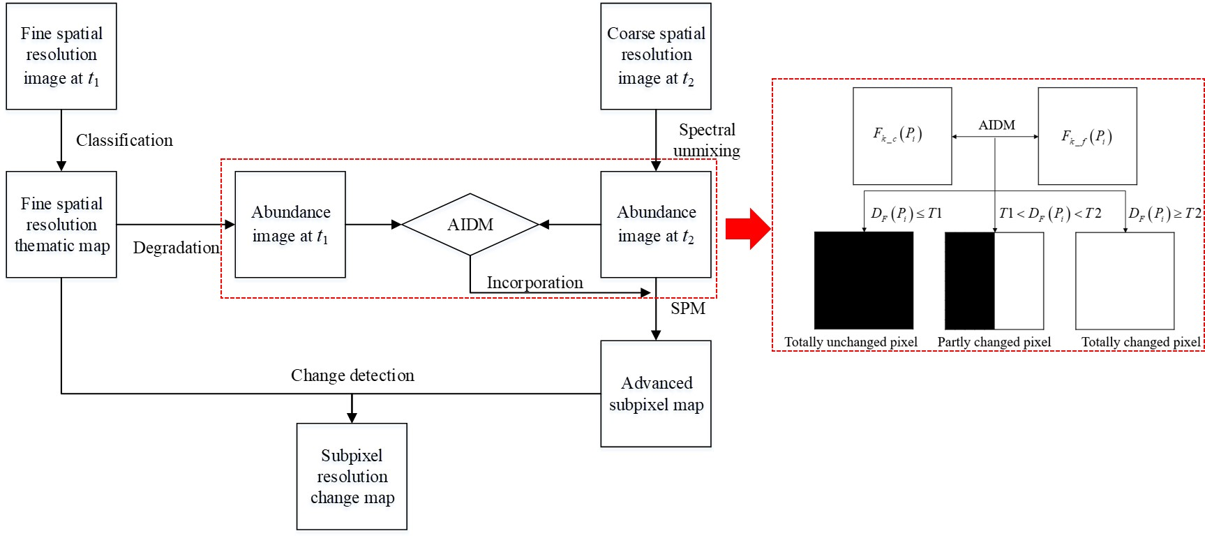
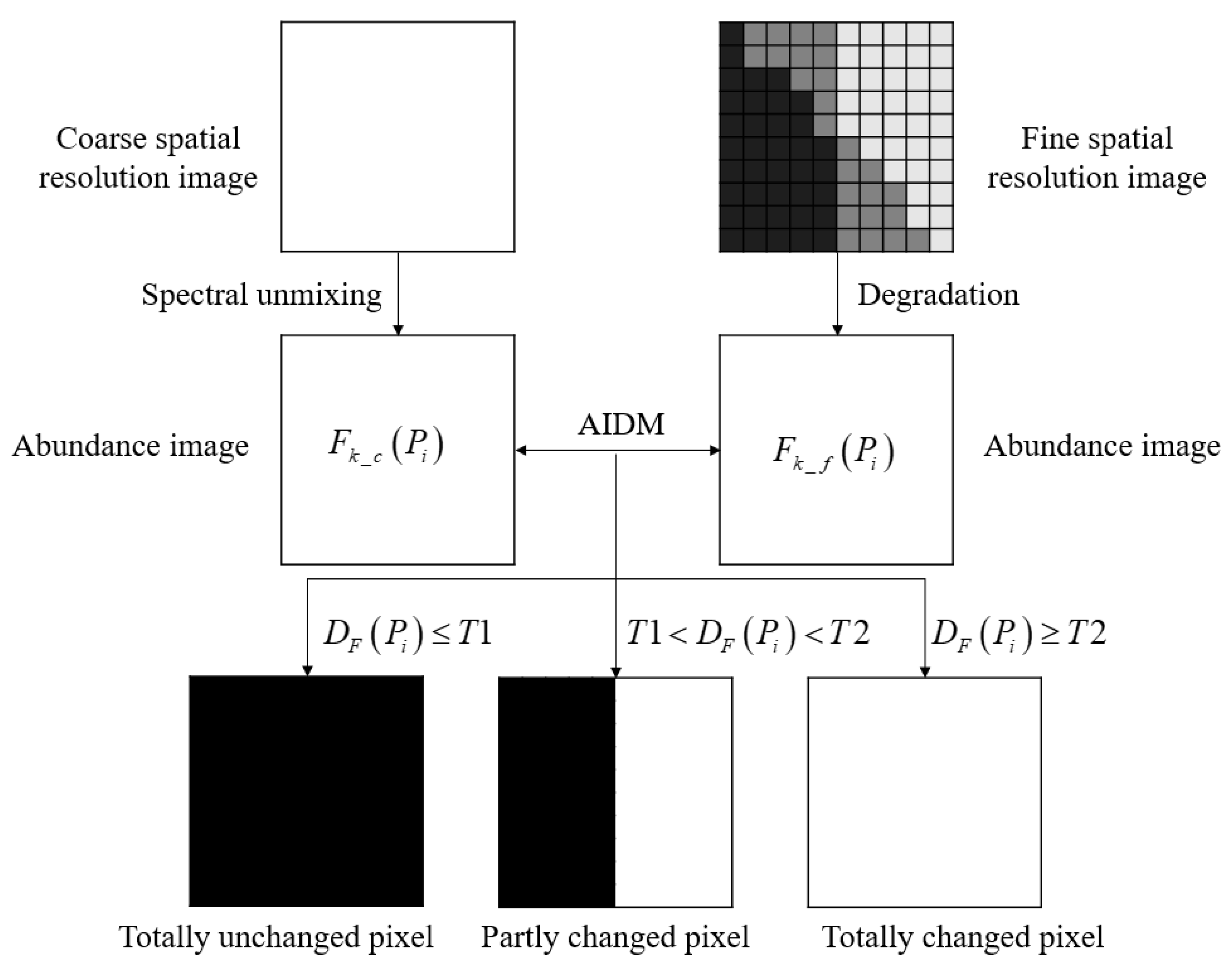
• If $D_F\left(P_i\right)\le T1$, there is no change for all classes within $P_i$. Consequently, the spatial distribution of the thematic map at t₂ is the same as that at t₁. More specifically, the RBF-based SPM result can be improved by repeating the fine thematic map at t₁.
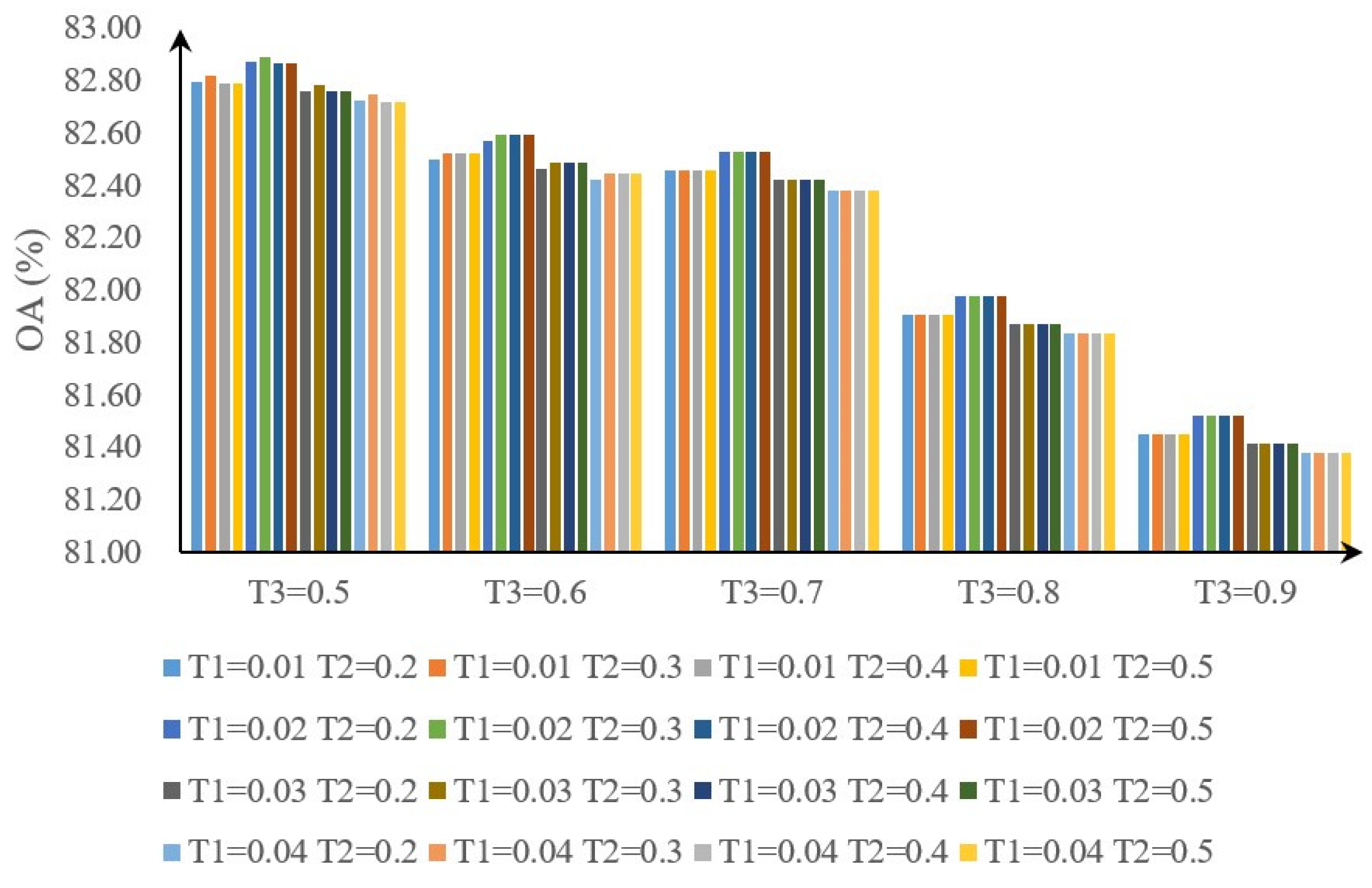
• If $D_F\left(P_i\right)\ge T2$, it is totally changed between bi-temporal images within $P_i$. In this condition, we need to make further judgments. If $F_{u\_c}\left(P_i\right)>T3$ (u = 1, 2, …, q; T3 is a threshold parameter), it indicates that the thematic map at t₂ within $P_i$ belongs to class u, then the RBF-based SPM result can be improved by replacing it to class u. Otherwise, the SPM result can be directly generated by RBF-based SPM method.
• If $T1<D_F\left(P_i\right)<T2$, it is indicated that there are partial changes within $P_i$. In this condition, further judgments on the abundance image cannot be made, and RBF-based SPM method is conducted to obtain the SPM result.

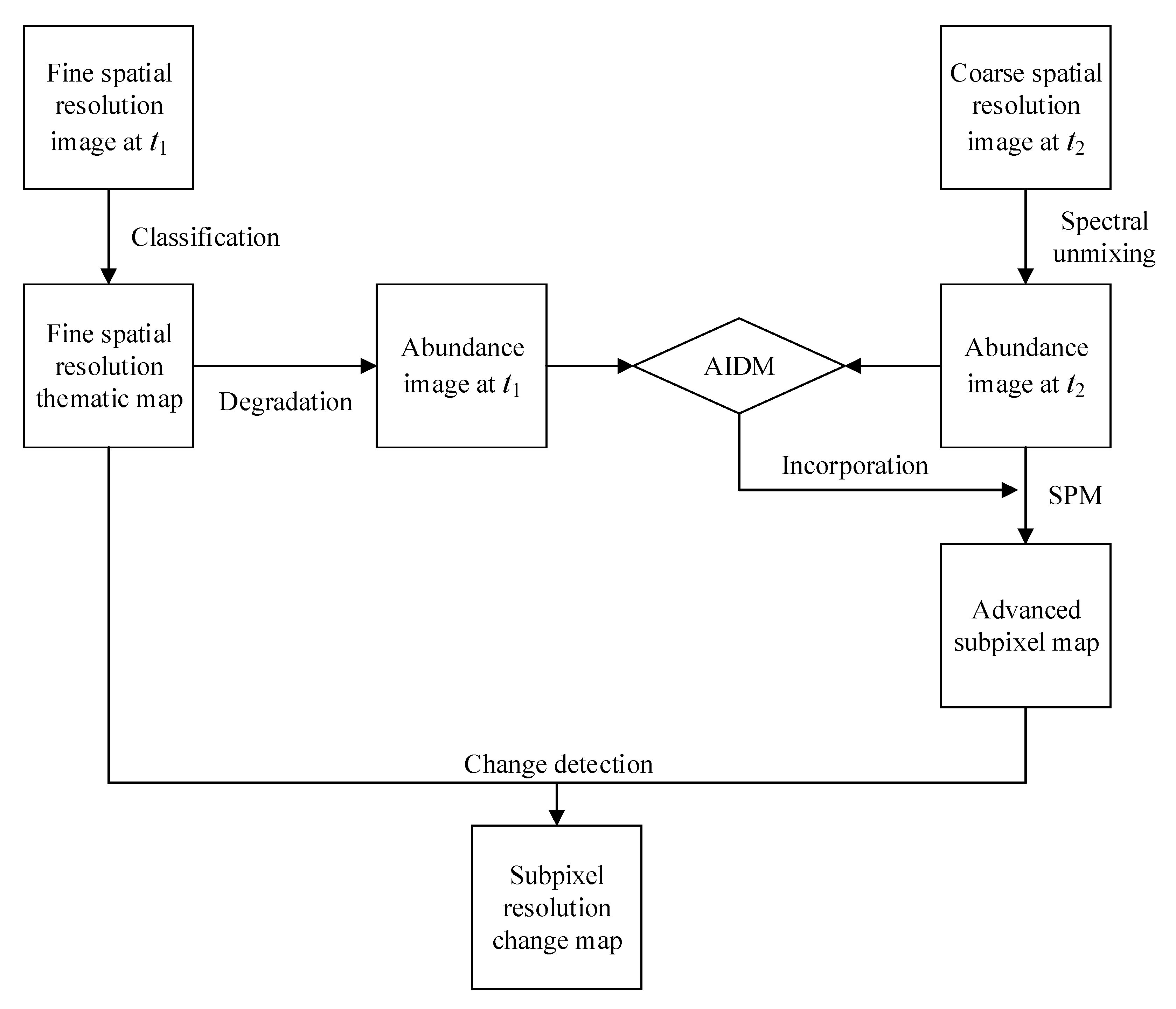
2.5. RBF-Based SPM for Subpixel Change Detection with AIDM

According to the proposed AIDM, the SPM result based on RBF is improved by utilizing the fine spatial resolution thematic map and enhances the performance of subpixel change detection. Therefore, a new subpixel change detection method based on RBF-SPM is proposed in this section. As shown in Figure 4, the proposed method broadly consists of four steps.

(1) Abundance image generation. For the coarse spatial resolution image at t₂, the spectral unmixing method is conducted to generate the abundance image $F_{k\_c}\left(P_i\right)$. For the fine image at t₁, the remote sensing image classification method is performed to obtain the fine spatial resolution thematic map. Then the degradation procedure is accomplished to generate the abundance image $F_{k\_f}\left(P_i\right)$ using the fine spatial resolution thematic map. Note that the degradation procedure is achieved according to the zoom factor S to ensure $F_{k\_c}\left(P_i\right)$ and $F_{k\_f}\left(P_i\right)$ have the same size.

(2) AIDM incorporation. For the generated $F_{k\_c}\left(P_i\right)$ and $F_{k\_f}\left(P_i\right)$, the proposed AIDM is applied to yield three kinds of changed pixels, namely, totally unchanged pixels, partly changed pixels and totally changed pixels.

(3) SPM. RBF-based SPM with the AIDM is accomplished in this step. Based on the abundance image at t₂ generated by spectral unmixing, pixels within the totally unchanged region are modified by repeating the fine thematic map at t₁. For the pixels within the totally changed region, a further process is conducted by comparing it with T3, then the SPM result can be enhanced by replacing it with the classes that meet the threshold condition. For pixels in the partly changed region, RBF-based SPM is performed to generate a subpixel map. Finally, the advanced subpixel map is obtained.

(4) Change detection. Subpixel resolution change detection is performed between the advanced subpixel map and the fine spatial resolution thematic map to produce the final subpixel resolution change map.

3. Experimental Results and Discussion

To evaluate the performance of the proposed subpixel change detection method, two datasets were tested for comparing the conventional RBF-based subpixel change detection and the proposed method. The parameters of the RBF method were set as follows according to the related paper [36]: the parameter a was set to 10, and the neighborhood window was set to 5.

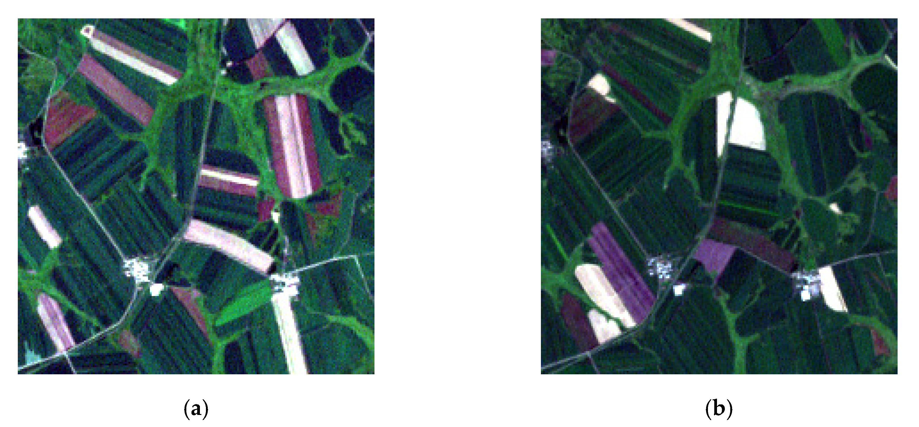
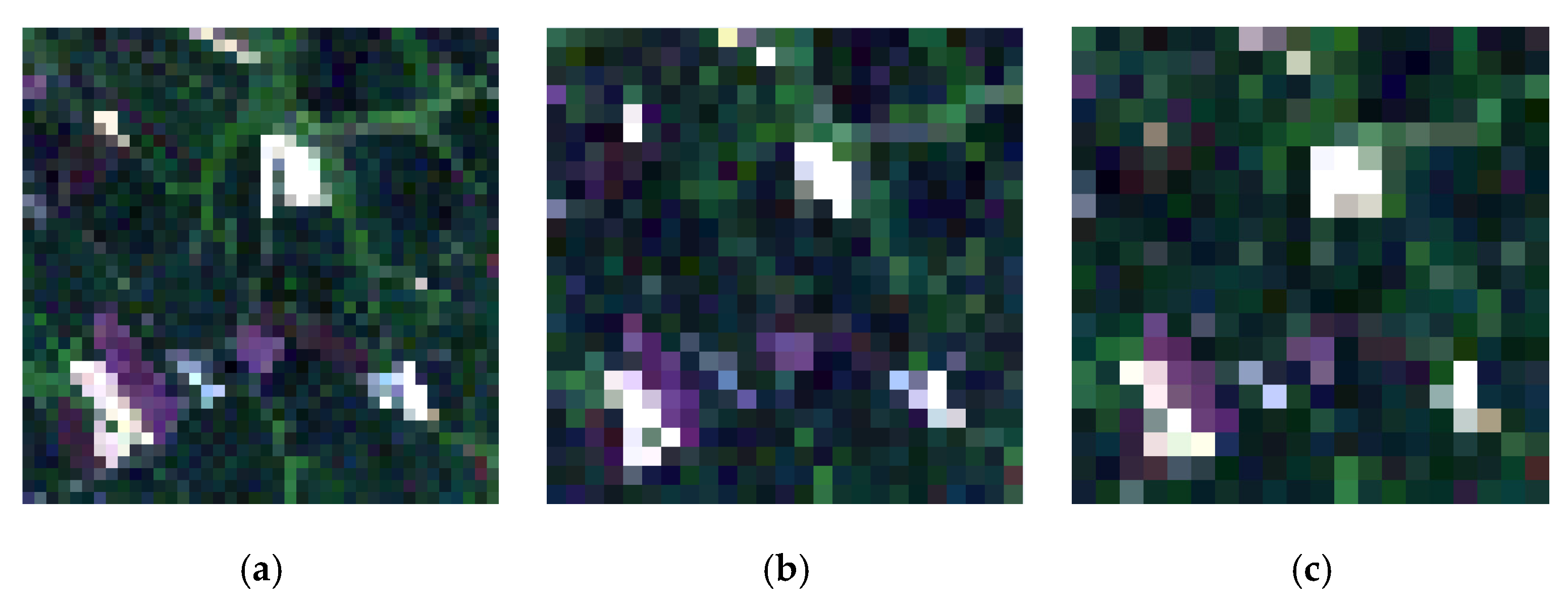
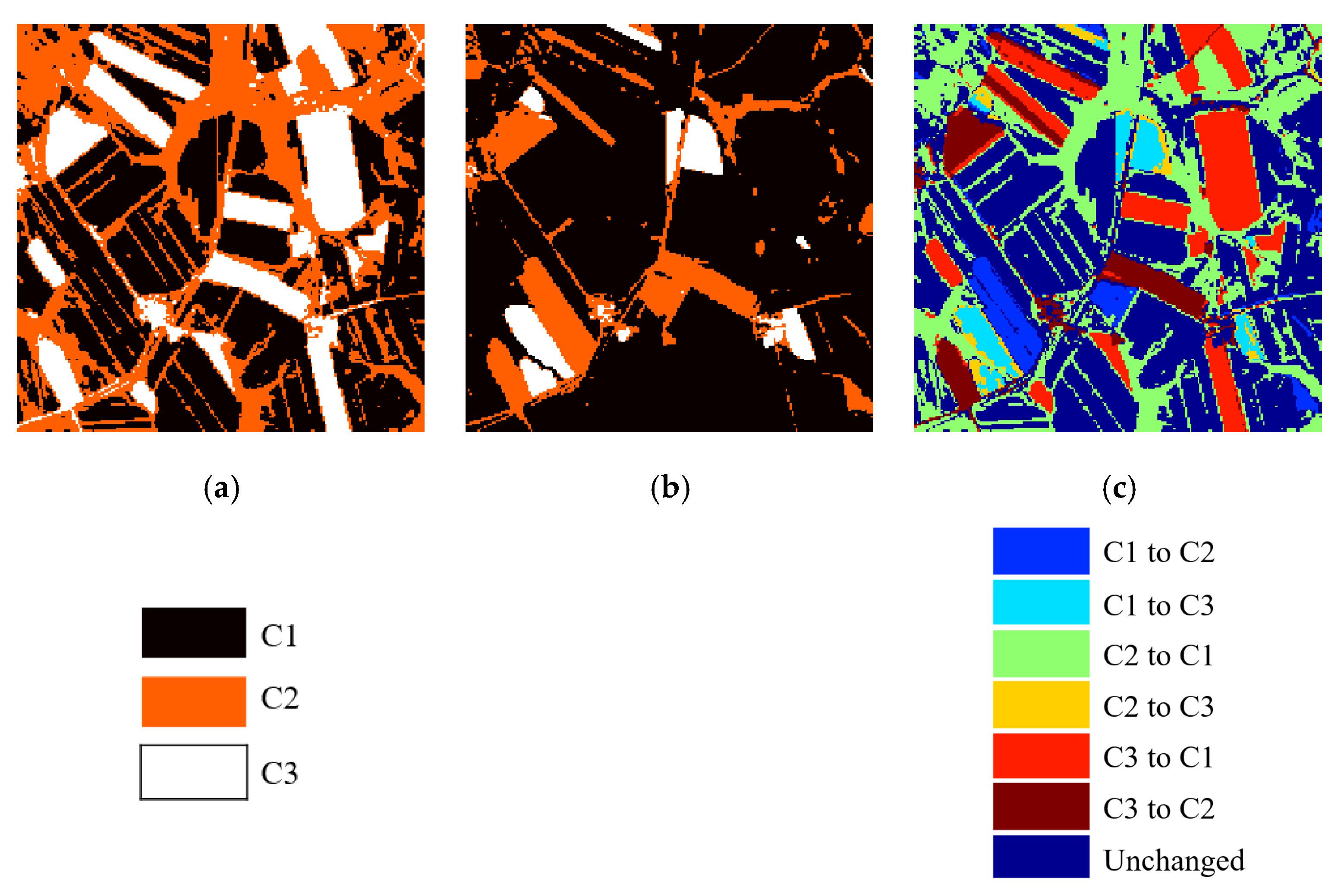
3.1. Experiment A

In this experiment, two temporal images acquired by the Landsat-7 Enhanced Thematic Mapper Plus (ETM+) sensor were utilized to simulate the fine and coarse spatial resolution images for controlling the analysis. The spatial resolution of the two temporal images is 30 m. Specifically, the previous image was obtained in August 2001 in Liaoning Province, China, which was denoted as the fine spatial resolution image at t₁. Correspondingly, the following image was obtained in August 2002 to denote the coarse spatial resolution image at t₂ by degradation procedure. The degradation procedure was accomplished via an S × S mean filter to generate the coarse image. As shown in Figure 5, the two temporal Landsat-7 ETM+ images are shown in Figure 5a,b, respectively.

There are many benefits of using the existing fine spatial resolution image to simulate the coarse spatial resolution image by degradation procedure. First, the true subpixel resolution change map can be obtained by comparing the two temporal thematic maps yielded by the corresponding Landsat-7 ETM+ images. Using the true subpixel resolution change map, different subpixel change detection methods can be evaluated precisely. Second, the true abundance images can be acquired by degrading the two temporal thematic maps, and they are used to generate the SPM results without spectral unmixing errors. At last, the true subpixel map can be generated by the thematic map at t₂ to evaluate the performance of SPM methods.

The two temporal Landsat-7 ETM+ images include three classes of crops, which are denoted as C1, C2 and C3, and the size of this area is 200 × 200 pixels. To explore the influence of different zoom factors on subpixel change detection, the zoom factor S is set to 5, 8, 10 to generate the coarse spatial resolution image at t₂ in this experiment. The spatial resolutions are 150, 240 and 300 m, respectively. As shown in Figure 6, the synthetic coarse images are shown in Figure 6a–c.

The two temporal thematic maps can be obtained by all kinds of classification methods, such as unsupervised classification methods, supervised classification methods and manual visual interpretation. In order to guarantee the accuracy of the thematic map, manual visual interpretation is employed in this experiment. According to the spectral differences of the three classes of crops, the thematic maps including three land covers, namely, C1, C2 and C3, can be obtained. Furthermore, the subpixel resolution change map including six types of changes (e.g., C1 to C2, C1 to C3) can be generated by comparing the two temporal thematic maps. As shown in Figure 7, the thematic map at t₁ is shown in Figure 7a, the thematic map at t₂ is shown in Figure 7b and the true subpixel resolution change map, or, the reference change map, is shown in Figure 7c.

For the generated coarse spatial resolution images, the linear spectral mixing modeling is conducted to obtain the abundance image at t₂ (AI2), in which the SMACC method is applied to acquire the three types of endmembers for its simplicity. Then, the thematic map at t₁ is processed to generate the abundance image at t₁ (AI1) by degradation procedure. In order to evaluate the performance of the spectral unmixing method, the true abundance image at t₂ (TAI2) is acquired by degrading the thematic map at t₂. Note that AI1 and TAI2 are obtained by degradation procedure using the two temporal thematic maps, then they can be taken as the true abundance images. Three sets of abundance images with S = 5, 8 and 10 are shown in Figure 8. We can see that there are some differences between AI2 and TAI2 in Figure 8, and it demonstrates that the spectral unmixing error does exist.

After the generation of the abundance images at t₂, the conventional RBF-based SPM method (RBF1) and the proposed RBF-based SPM method with the AIDM (RBF-AIDM) are performed to produce the subpixel map. As shown in Figure 9, taking AI2 as input and setting T1 = 0.02, T2 = 0.3, T3 = 0.5 (the parameters are obtained by the experimental method), the SPM results can be generated using RBF1 and RBF-AIDM. In contrast, the SPM results (RBF-TAI2) can be achieved using TAI2 as input, and the results represent the RBF-based SPM results without the influence of spectral unmixing error. By comparing the three sets of SPM results with the thematic map at t₂ in Figure 7b, we can see that the SPM results based on RBF-TAI2 are better than those based on RBF1 and RBF-AIDM, and the phenomenon indicates that the spectral unmixing error had a deep influence on SPM results. Moreover, the SPM results based on RBF-AIDM have a greater performance than those based on RBF1, and it is shown that the proposed AIDM can decrease the influence of the spectral unmixing error effectively and improve the RBF-based SPM results.

Based on the aforementioned SPM results, the subpixel resolution change maps can be obtained by comparing the three sets of SPM results with the thematic map at t₁ in Figure 7a. As shown in Figure 10, the subpixel resolution change maps based on RBF1 are generated by comparing the RBF1-based subpixel maps and the thematic map at t₁. Similarly, the subpixel resolution change maps based on RBF-AIDM and RBF-TAI2 are generated by comparing the RBF-AIDM-based subpixel maps, and the RBF-TAI2-based subpixel maps with the thematic map at t₁, respectively. By comparing the three sets of subpixel change maps with the reference change map in Figure 7c, we can see that the subpixel resolution change maps based on RBF-TAI2 are better than those based on RBF1 and RBF-AIDM, and they indicate that the spectral unmixing error had a deep influence on subpixel change detection. Moreover, by comparing the subpixel resolution change maps based on RBF1 and RBF-AIDM, the results represent that RBF-AIDM-based subpixel resolution change maps have greater performance than those based on RBF1, and they indicate that the proposed AIDM can improve the RBF-based subpixel change detection.

For quantitative evaluation of the three sets of subpixel change detection results based on RBF1, RBF-AIDM and RBF-TAI2, the overall accuracy (OA) is used to evaluate the change detection performances. Additionally, two change detection error indexes are implemented to evaluate the influences of spectral unmixing error and SPM error. Here, we denote E1 as the change detection error generated by spectral unmixing error and E2 as the change detection error generated by the SPM stage.

Table 1. The quantitative evaluation of subpixel change detection based on the three methods.

CD OA	S = 5			S = 8			S = 10
	OA1	E1	E2	OA1	E1	E2	OA1	E1	E2
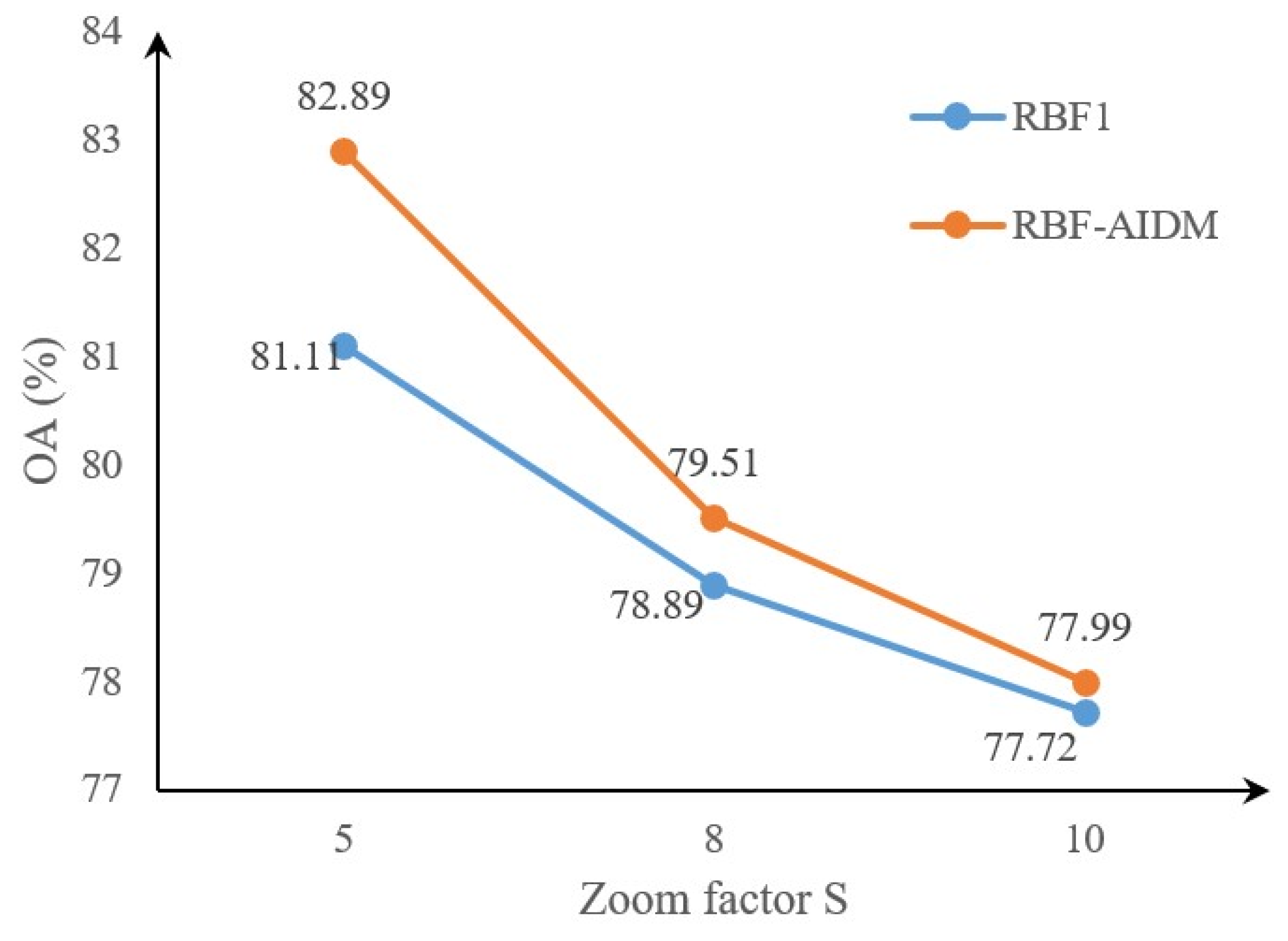
RBF1	81.11	13.09	5.8	78.89	12.78	8.33	77.72	12.06	10.22
RBF-AIDM	82.89	11.31	5.8	79.51	12.16	8.33	77.99	11.79	10.22
RBF-TAI2	94.20	/	5.8	91.67	/	8.33	89.78	/	10.22

shows the OA, E1 and E2 values of the three sets of subpixel change detection results. As shown in Table 1, the OA of RBF1, RBF-AIDM and RBF-TAI2 is 81.11%, 82.89 and 94.20% when S = 5, respectively. Hence, RBF-TAI2 outperforms RBF1 and RBF-AIDM in subpixel change detection performance, and it indicates that the spectral unmixing error has a deep influence on subpixel change detection considering that the subpixel change detection results based on RBF-TAI2 are generated without the spectral unmixing stage. By comparing the subpixel change detection results based on RBF1 and RBF-AIDM, we can see that the OA of RBF-AIDM improves 1.78% over RBF1, and it demonstrates that the proposed method is effective in improving the subpixel change detection performance.

When it comes to the zoom factor S, we can see that the subpixel change detection results of RBF1, RBF-AIDM and RBF-TAI2 with S = 8 and 10 are coincident with S = 5. Especially, as shown in Figure 11, there is such a rule that the OA decreases as S increases. It represents that the greater the spatial resolution difference between two temporal images, the lower the subpixel change detection accuracy. Moreover, as S increases, the E1 gradually decreases, and the E2 gradually increases. The phenomenon indicates that the influence of spectral unmixing error for subpixel change detection is great when the spatial resolution difference between the two temporal images is relatively small.

To explore the effect of the aforementioned three threshold parameters (i.e., T1, T2 and T3) on subpixel change detection results, the proposed RBF-AIDM method is conducted on the Landsat-7 ETM+ images to produce the change detection results using a set of parameters. Around the aforementioned parameters employed in experiment A, let set T1 = 0.01, 0.02, 0.03 and 0.04; T2 = 0.2, 0.3, 0.4 and 0.5; T3 = 0.5, 0.6, 0.7, 0.8 and 0.9. Figure 12 shows the subpixel change detection OA of the proposed RBF-AIDM method using different parameters when S = 5. From Figure 12, three observations can be made. First, the subpixel change detection OA based on the RBF-AIDM method using all of the selected parameters is better than the conventional RBF1 method, and the results indicate that the proposed RBF-AIDM method can effectively improve the subpixel change detection result, and it is insensitive to parameter selection in the same time. Second, the OA can achieve the maximum when T1 = 0.02, T2 = 0.3 and T3 = 0.5, and the OA will decrease when the three parameters decrease or increase. The phenomenon indicates that the optimal parameters are existing and different parameters will have an effect on the subpixel change detection result.

3.2. Experiment B

In this experiment, a set of Landsat-MODIS images, including two temporal Landsat-8 Operational Land Imager (OLI) images and one MODIS image, was used to test the proposed subpixel change detection method for a real case. The studied site is a 24 km × 24 km area of tropical water covering the city of Hefei, China. The previous Landsat-8 OLI image was acquired in October 2014, which was denoted as the fine spatial resolution image at t₁. The following MODIS image was acquired in October 2018, which was denoted as the coarse spatial resolution image at t₂. To facilitate accuracy evaluation, one Landsat-8 OLI image acquired in November 2018 was used as the reference. Note that the latter Landsat-8 OLI image is only used to evaluate the change detection accuracy as the fine spatial resolution image and is not necessary for the proposed subpixel change detection method.

Considering that the spatial resolution of the Landsat-8 OLI image is 30 m, the SPM method was conducted on the MODIS image to produce the 30 m spatial resolution land cover map. Because the spatial resolution of the MODIS image is 500 m, the nearest neighbor algorithm is used to resample the original MODIS image to 480 m for satisfying the zoom factor. Then, the zoom factor of SPM for the MODIS image is set to 16 to predict a land cover map at 30 m spatial resolutions. The spatial size of the Landsat image is 800 × 800 pixels, and the MODIS image is 50 × 50 pixels, Figure 13 shows the three images.

As with experiment A, the manual visual interpretation was conducted on the two temporal Landsat-8 OLI images to produce the corresponding thematic maps at t₁ and t₂. For the studied tropical water area, two main classes, i.e., water and non-water, were applied as the types of classification, and two change types, namely, water to non-water and non-water to water, were detected. For each 30 m Landsat-8 OLI image, the pixels were expected to be pure materials. Figure 14 shows the two temporal thematic maps, in which Figure 14a shows the thematic map at t₁ and Figure 14b shows the thematic map at t₂. In addition, Figure 14c shows the reference change map by comparing the two temporal thematic maps.

Before executing the SPM method, the linear spectral mixing modeling is conducted on the MODIS image to produce the abundance image at t₂. As with the aforementioned thematic map, the endmembers within the abundance image include two types, namely, water and non-water. For the Landsat-8 OLI image, the degradation procedure is performed to produce the abundance image at t₁. Figure 15 displays the two temporal abundance images. As shown in Figure 15, the two images on the left denote the abundance images of water and non-water based on the Landsat-8 OLI image at t₁, and the two images on the right denote the abundance images of water and non-water based on the MODIS image at t₂.

After generating the abundance images at t₂ based on MODIS image, the conventional RBF-based SPM method and the proposed RBF-based SPM method, namely, RBF1 and RBF-AIDM, are performed to produce the subpixel map. As shown in Figure 15, taking the aforementioned abundance image as input and setting T1 = 0.02, T2 = 0.3, T3 = 0.5, the SPM results can be generated using RBF1 and RBF-AIDM. By comparing the two SPM results with the thematic map at t₂ in Figure 14b, we can see that the SPM result based on RBF-AIDM is better than that based on RBF1, and the phenomenon indicates that the proposed AIDM can decrease the influence of spectral unmixing error effectively and improve the RBF-based SPM result.

Using the aforementioned SPM results, the subpixel resolution change maps can be obtained by comparing the two SPM results with the thematic map at t₁. As shown in Figure 16, the subpixel resolution change maps based on RBF1 and RBF-AIDM are generated by comparing the RBF1-based subpixel map and RBF-AIDM-based subpixel map with the thematic map at t₁, respectively. By comparing the two subpixel change maps with the reference change map in Figure 14c, the results represent that RBF-AIDM-based subpixel resolution change maps have a greater performance than those based on RBF1, and they indicate that the proposed AIDM can improve the RBF-based subpixel change detection. Moreover, the quantitative evaluation of the two subpixel resolution change maps based on RFB1 and RBF-AIDM demonstrates the effectiveness of the proposed method. Specifically, the OA of subpixel resolution change map based on RBF1 is 89.04%, and the OA of subpixel resolution change map based on RBF-AIDM is 91.76%. By comparing the subpixel change detection results based on RBF1 and RBF-AIDM, we can see that the OA of RBF-AIDM improve 2.72% over RBF1, and it demonstrates that the proposed method is effective in improving the subpixel change detection performance.

4. Conclusions

Land cover change detection from remote sensing images has become a research focus in the remote sensing field, and the change detection results are required to be obtained at a fine spatial resolution for detecting sufficient details in recent years. Considering the reality that sensors with fine spatial resolution usually have a long revisit time, and sensors with fine temporal resolution always have a low spatial resolution in contrast, the subpixel change detection is widely utilized to produce fine spatial resolution change detection results.

In this paper, we proposed a new RBF-based SPM method for subpixel change detection with the AIDM. In this method, the AIDM is designed using the two temporal abundance images to reduce the impact of the spectral unmixing error for subpixel change detection. Specifically, this method can be described as follows. First, the fine and coarse spatial resolution images are used to generate the fine spatial resolution change map. The fine spatial resolution image is processed to obtain the fine spatial resolution thematic map by image classification procedure, then the corresponding abundance image is generated by degradation using the fine spatial resolution thematic map. Meanwhile, the coarse spatial resolution image is utilized to produce the abundance image using linear spectral mixing modeling. Second, the proposed RBF-AIDM-based SPM method is conducted on the abundance image generated by spectral unmixing to produce the SPM result. In this procedure, the designed AIDM is used to enhance the RBF-based SPM by comparing the two temporal abundance images, in which the spatial distribution of the fine spatial resolution thematic map is borrowed to improve the SPM result. Lastly, the subpixel change map is obtained by comparing the fine spatial resolution thematic map with the SPM result.

The synthetic image experiment based on Landsat-7 ETM+ sensor is undertaken to validate the proposed RBF-AIDM method for controlling the analysis. The experiment result indicates that the spectral unmixing error has a deep influence on the subpixel change detection, and the proposed RBF-AIDM method can decrease the influence of the spectral unmixing error effectively and improve the subpixel change detection results. In addition, two temporal Landsat–MODIS images are used to test the proposed subpixel change detection method for a real case, and the experiment result confirms that the proposed method has the capability of borrowing the fine spatial distribution from the fine spatial resolution thematic map and improving the subpixel change detection results. In future research, more SPM algorithms will be explored for subpixel change detection and automatic determination of parameters will be studied.

References

- Singh, A. Review Article Digital change detection techniques using remotely-sensed data. Int. J. Remote Sens. 1989, 10, 989–1003. [Google Scholar] [CrossRef]
- Lu, D.; Mausel, P.; Brondizio, E.; Moran, E. Change detection techniques. Int. J. Remote Sens. 2004, 25, 2365–2401. [Google Scholar] [CrossRef]
- Bruzzone, L.; Bovolo, F. A novel framework for the design of change- detection systems for very-high-resolution remote sensing images. Proc. IEEE 2013, 101, 609–630. [Google Scholar] [CrossRef]
- Hussain, M.; Chen, D.; Cheng, A.; Wei, H.; Stanley, D. Change detection from remotely sensed images: From pixel-based to object-based approaches. ISPRS J. Photogramm. Remote Sens. 2013, 80, 91–106. [Google Scholar] [CrossRef]
- Tewkesbury, A.P.; Comber, A.J.; Tate, N.J.; Lamb, A.; Fisher, P.F. A critical synthesis of remotely sensed optical image change detection techniques. Remote Sens. Environ. 2015, 160, 1–14. [Google Scholar] [CrossRef]
- Johansen, K.; Arroyo, L.A.; Phinn, S.; Witte, C. Comparison of Geo-Object Based and Pixel-Based Change Detection of Riparian Environments using High Spatial Resolution Multi-Spectral Imagery. Photogramm. Eng. Remote Sens. 2010, 76, 123–136. [Google Scholar] [CrossRef]
- Mandanici, E.; Bitelli, G. Multi-Image and Multi-Sensor Change Detection for Long-Term Monitoring of Arid Environments with Landsat Series. Remote Sens. 2015, 7, 14019–14038. [Google Scholar] [CrossRef]
- Atzberger, C. Advances in remote sensing of agriculture: Context description, existing operational monitoring systems and major information needs. Remote Sens. 2013, 5, 949–981. [Google Scholar] [CrossRef]
- Du, P.; Liu, S.; Gamba, P.; Tan, K.; Xia, J. Fusion of difference images for change detection over urban areas. IEEE J. Sel. Top. Appl. Earth Obs. Remote Sens. 2012, 5, 1076–1086. [Google Scholar] [CrossRef]
- Hebel, M.; Arens, M.; Stilla, U. Change detection in urban areas by object-based analysis and on-the-fly comparison of multi-view ALS data. ISPRS J. Photogramm. Remote Sens. 2013, 86, 52–64. [Google Scholar] [CrossRef]
- Desclee, B.; Bogaert, P.; Defourny, P. Forest change detection by statistical object-based method. Remote Sens. Environ. 2006, 102, 1–11. [Google Scholar] [CrossRef]
- Chehata, N.; Orny, C.; Boukir, S.; Guyon, D.; Wigneron, J.P. Object-based change detection in wind storm-damaged forest using high-resolution multispectral images. Int. J. Remote Sens. 2014, 35, 4758–4777. [Google Scholar] [CrossRef]
- Fung, T. An assessment of TM imagery for land-cover change detection. IEEE Trans. Geosci. Remote Sens. 1990, 28, 681–684. [Google Scholar] [CrossRef]
- Rignot, E.J.; Van Zyl, J.J. Change detection techniques for ERS-1 SAR data. IEEE Trans. Geosci. Remote Sens. 1993, 31, 896–906. [Google Scholar] [CrossRef]
- Johnson, R.D.; Kasischke, E. Change vector analysis: A technique for the multispectral monitoring of land cover and condition. Int. J. Remote Sens. 1998, 19, 411–426. [Google Scholar] [CrossRef]
- Bruzzone, L.; Prieto, D.F. Automatic analysis of the difference image for unsupervised change detection. IEEE Trans. Geosci. Remote Sens. 2000, 38, 1171–1182. [Google Scholar] [CrossRef]
- He, P.; Shi, W.; Zhang, H.; Hao, M. A novel dynamic threshold method for unsupervised change detection from remotely sensed images. Remote Sens. Lett. 2014, 5, 396–403. [Google Scholar] [CrossRef]
- Ghosh, A.; Mishra, N.S.; Ghosh, S. Fuzzy clustering algorithms for unsupervised change detection in remote sensing images. Inf. Sci. 2011, 181, 699–715. [Google Scholar] [CrossRef]
- Hao, M.; Zhang, H.; Shi, W.; Deng, K. Unsupervised change detection using fuzzy c-means and MRF from remotely sensed images. Remote Sens. Lett. 2013, 4, 1185–1194. [Google Scholar] [CrossRef]
- Foody, G. Monitoring the magnitude of land-cover change around the southern limits of the Sahara. Photogramm. Eng. Remote Sens. 2001, 67, 841–847. [Google Scholar] [CrossRef]
- Yuan, F.; Sawaya, K.E.; Loeffelholz, B.C.; Bauer, M.E. Land cover classification and change analysis of the Twin Cities (Minnesota) Metropolitan Area by multitemporal Landsat remote sensing. Remote Sens. Environ. 2005, 98, 317–328. [Google Scholar] [CrossRef]
- Melgani, F.; Bruzzone, L. Classification of hyperspectral remote sensing images with support vector machines. IEEE Trans. Geosci. Remote Sens. 2004, 42, 1778–1790. [Google Scholar] [CrossRef]
- Mantero, P.; Moser, G.; Serpico, S.B. Partially supervised classification of remote sensing images through SVM-based probability density estimation. IEEE Trans. Geosci. Remote Sens. 2005, 43, 559–570. [Google Scholar] [CrossRef]
- Wang, M.C.; Zhang, H.M.; Sun, W.W.; Li, S.; Wang, F.Y.; Yang, G.D. A Coarse-to-Fine Deep Learning Based Land Use Change Detection Method for High-Resolution Remote Sensing Images. Remote Sens. 2020, 12, 1933. [Google Scholar] [CrossRef]
- Song, A.; Choi, J. Fully Convolutional Networks with Multiscale 3D Filters and Transfer Learning for Change Detection in High Spatial Resolution Satellite Images. Remote Sens. 2020, 12, 799. [Google Scholar] [CrossRef]
- Lu, D.; Batistella, M.; Moran, E. Multitemporal spectral mixture analysis for Amazonian land-cover change detection. Can. J. Remote Sens. 2004, 30, 87–100. [Google Scholar] [CrossRef]
- Yokoya, N.; Zhu, X.X.; Plaza, A. Multisensor coupled spectral unmixing for time-series analysis. IEEE Trans. Geosci. Remote Sens. 2017, 55, 2842–2857. [Google Scholar] [CrossRef]
- Wang, Q.; Shi, W.; Atkinson, P.M.; Li, Z. Land Cover Change Detection at Subpixel Resolution with a Hopfield Neural Network. IEEE J. Sel. Top. Appl. Earth Obs. Remote Sens. 2015, 8, 1339–1352. [Google Scholar] [CrossRef]
- Wu, K.; Zhong, Y.; Wang, X.; Sun, W. A Novel Approach to Subpixel Land-Cover Change Detection Based on a Supervised Back-Propagation Neural Network for Remotely Sensed Images with Different Resolutions. IEEE Geosci. Remote Sens. Lett. 2017, 14, 1750–1754. [Google Scholar] [CrossRef]
- He, D.; Zhong, Y.F.; Zhang, L.P. Spectral-Spatial-Temporal MAP-Based Sub-Pixel Mapping for Land-Cover Change Detection. IEEE Trans. Geosci. Remote Sens. 2020, 58, 1696–1717. [Google Scholar] [CrossRef]
- Ling, F.; Du, Y.; Xiao, F.; Li, X. Subpixel land cover mapping by integrating spectral and spatial information of remotely sensed imagery. IEEE Geosci. Remote Sens. Lett. 2012, 9, 408–412. [Google Scholar] [CrossRef]
- Wang, Q.; Shi, W.; Zhang, H. Class Allocation for Soft-Then-Hard Subpixel Mapping Algorithms with Adaptive Visiting Order of Classes. IEEE Geosci. Remote Sens. Lett. 2014, 11, 1494–1498. [Google Scholar] [CrossRef]
- Wang, Q.; Shi, W.; Atkinson, P.M. Sub-pixel mapping of remote sensing images based on radial basis function interpolation. ISPRS J. Photogramm. Remote Sens. 2014, 92, 1–15. [Google Scholar] [CrossRef]
- Wang, Q.; Zhang, C.; Tong, X.; Atkinson, P.M. General solution to reduce the point spread function effect in subpixel mapping. Remote Sens. Environ. 2020, 251, 112054. [Google Scholar] [CrossRef]
- Wang, Q.; Zhang, C.; Atkinson, P.M. Sub-pixel mapping with point constraints. Remote Sens. Environ. 2020, 244, 111817. [Google Scholar] [CrossRef]
- Wang, Q.; Atkinson, P.M.; Shi, W. Fast Subpixel Mapping Algorithms for Subpixel Resolution Change Detection. IEEE Trans. Geosci. Remote Sens. 2015, 53, 1692–1706. [Google Scholar] [CrossRef]
- Heinz, D.C.; Chang, C.I. Fully constrained least squares linear spectral mixture analysis method for material quantification in hyperspectral imagery. IEEE Trans. Geosci. Remote Sens. 2001, 39, 529–545. [Google Scholar] [CrossRef]
- Carpenter, G.A.; Gopal, S.; Macomber, S.; Martens, S.; Woodcock, C.E. A neural network method for mixture estimation for vegetation mapping. Remote Sens. Environ. 1999, 70, 138–152. [Google Scholar] [CrossRef]
- Wang, L.G.; Jia, X.P. Integration of Soft and Hard Classifications Using Extended Support Vector Machines. IEEE Geosci. Remote Sens. Lett. 2009, 6, 543–547. [Google Scholar] [CrossRef]
- Bastin, L. Comparison of fuzzy c-means classification, linear mixture modelling and MLC probabilities as tools for unmixing coarse pixels. Int. J. Remote Sens. 1997, 18, 3629–3648. [Google Scholar] [CrossRef]
- Gruninger, J.H.; Ratkowski, A.J.; Hoke, M.L. The sequential maximum angle convex cone (SMACC) endmember model. Proc. SPIE 2004, 5425, 1–14. [Google Scholar] [CrossRef]
- Zortea, M.; Plaza, A. A Quantitative and Comparative Analysis of Different Implementations of N-FINDR: A Fast Endmember Extraction Algorithm. IEEE Geosci. Remote Sens. Lett. 2009, 6, 787–791. [Google Scholar] [CrossRef]
- Wang, Q.; Shi, W.; Wang, L. Allocating classes for soft-then-hard subpixel mapping algorithms in units of class. IEEE Trans. Geosci. Remote Sens. 2014, 52, 2940–2959. [Google Scholar] [CrossRef]