KVGCN: A KNN Searching and VLAD Combined Graph Convolutional Network for Point Cloud Segmentation

Abstract

Semantic segmentation of the sensed point cloud data plays a significant role in scene understanding and reconstruction, robot navigation, etc. This work presents a Graph Convolutional Network integrating K-Nearest Neighbor searching (KNN) and Vector of Locally Aggregated Descriptors (VLAD). KNN searching is utilized to construct the topological graph of each point and its neighbors. Then, we perform convolution on the edges of constructed graph to extract representative local features by multiple Multilayer Perceptions (MLPs). Afterwards, a trainable VLAD layer, NetVLAD, is embedded in the feature encoder to aggregate the local and global contextual features. The designed feature encoder is repeated for multiple times, and the extracted features are concatenated in a jump-connection style to strengthen the distinctiveness of features and thereby improve the segmentation. Experimental results on two datasets show that the proposed work settles the shortcoming of insufficient local feature extraction and promotes the accuracy (mIoU 60.9% and oAcc 87.4% for S3DIS) of semantic segmentation comparing to existing models.

1. Introduction

As one of the key technologies for scene understanding, semantic segmentation [1,2,3] of 3D point clouds plays fundamental roles in the fields of 3D reconstruction, autonomous driving, and robotics. Vehicles in autonomous driving applications need to interpret the objects (e.g., pedestrians and cars) and their kinestates in the outdoor scenes before making reliable decisions. For a robot, reconstructing and parsing the models of surrounding environments is the premise of navigation and object manipulation. Unlike 2D images, point clouds are unstructured, unevenly distributed, and large in data volume, making them difficult to process analyze by the conventional methods. Great attention has been paid to achieving reliable semantic segmentation of point clouds in deep learning style. However, how to effectively learn presentative features from unorganized point clouds is still a challenging problem.

In order to solve the difficulty of feature learning caused by disordered point clouds, a number of works [4,5,6,7,8,9,10] preprocess the 3D point cloud data to a normalized 2D or 3D representation, such as voxelization and multi-view projection. However, projection causes information loss, and the 3D convolution after voxelization brings greater computational cost. Another type of work, on the other hand, uses the original point clouds as input and conducts end-to-end learning, such as the pioneering work PointNet [11], the upgraded PointNet++ [12], and other new deep networks [13,14,15,16,17,18,19,20]. They all directly deal with the unordered point clouds, and learn global and local features to realize the classification and segmentation. These works have achieved excellent results, yet difficulties still exist in the processing of point clouds [21]. The effective local geometric feature correspondence cannot be established, and the information between the points cannot be well utilized, which results in low accuracy of semantic segmentation.

To solve the above issues, this work mainly considers two aspects: how to learn features from the local structures and how to aggregate the local and global information. In this paper, we propose the K-nearest neighbor searching (KNN) and Vector of Locally Aggregated Descriptors (VLAD) [22] combined Graph Convolutional Network (KVGCN) to learn point cloud features from the topological graph constructed by each point and its K-nearest neighbors. Specifically, it performs convolution on the edges of constructed graph to extract representative local features by multiple MLPs, followed by two different pooling operations to compensate information loss. Then, the VLAD layer is embedded in the feature encoding block to aggregate local and global contextual features. Furthermore, the designed feature encoding block is repeated multiple times and the extracted features are concatenated in a jump connection style to strengthen the ability of network and thereby improve the accuracy of semantic segmentation. Our key contributions are as follows.

• We propose an edge convolution on the constructed KNN graph to encode the local features. The query point denotes the global position and the edges, namely, the relative positions of the query point and its neighbors, represent the local geometry. By concatenating this information, representative features can be achieved via edge convolution.
• We employ max pooling and average pooling as the symmetric functions, and because VLAD layer is symmetric, the proposed network guarantees invariance to the point order.
• By embedding the VLAD layer in the feature encoding block, we construct an enhanced feature merging encoder which effectively aggregate the local features and the global contextual information. The segmentation in dense region or confusable region improves.
• Experimental results on two datasets show that KVGCN achieves comparable or superior performance compared with state-of-the-art methods.

The rest of this work is organized as follows. Section 2 classifies and discusses the related work. Section 3 describes details of the proposed KGCN and KVGCN segmentation networks. Experimental evaluations and discussions are performed in Section 4 and Section 5. Then, Section 6 concludes this work.

2. Related Work

Before the deep learning era, most researchers followed the traditional routine of “segmenting then labeling” in point cloud segmentation. However, with the growing scale of 3D data, the workload of traditional methods increases rapidly, resulting in low efficiency of segmenting [23,24,25,26]. On the other hand, the deep learning-based methods can improve the accuracy and efficiency of semantic segmentation [27]. At present, the semantic segmentation models based on deep learning can be divided into two main categories.

2.1. Networks with Preprocessings

This type of model presents the 3D data in multi-view renderings or voxels. The multi-view convolutional neural network (MV-CNN) was first applied to 3D shape recognition [4], rendering 3D data from multiple visions into 2D images as input to 2D CNNs. Kalogerakis et al. [6] propose a more complex multi-view rendering framework based on the multi-view CNNs. The MV-RNN [7] model successfully applies a Recurrent Neural Network (RNN) to the 3D image field, which treats multi-view image sequences as time series and uses RNN to learn features from images.

Point cloud voxelization converts the irregular point cloud into the regular 3D voxelized representation. Qi et al. [9] propose a volumetric convolution neural network model (volumetric CNN), which was developed based on the 2D CNNs. Maturana et al. [5] develop the VoxNet model, which divides the 3D space into regular 3D voxel grids and applies it to the revised 3D CNN model. However, the biggest disadvantage of this method is that the higher resolution of the voxelization, the faster the memory and computing consumption increase. What is worse, the increase in the resolution of the voxel causes many empty voxel grids, so the calculations consumed in this part are wasteful. In order to reduce this waste, 3D CNNs based on rough resolution [8] seem to be a solution, but in turn lead to greater quantization errors.

Some researchers also propose other works to reduce the huge consumption of memory and computation of voxelized CNNs, for instance, the Kd-Net [28] and OctNet [29]. These algorithms are all tree-based models that can perform high-resolution voxel learning on point clouds. These models try to ignore empty voxel grids and focus on the information-rich grids, but are difficult to implement and expressiveness limited. Qi et al. [9] compare the recognition performance of the volumetric methods and multi-view presentation. Compared with voxel representation, multi-view rendering lowers the calculation cost, but causes information loss.

2.2. End-to-End Learning Networks

In order to make full use of the information of point clouds, many researchers abandoned the preprocessing and tried to learn the point clouds end-to-end. A groundbreaking work, PointNet [11], is completed for unordered point clouds. It directly processes point clouds and uses the pooling layer to extract the global point features. On several different datasets, PointNet achieves advanced performance in 3D classification and semantic segmentation. However, there is a drawback that the PointNet lacks local feature representation. Therefore, the authors propose an improved model, PointNet++ [12], which applies a fast point sampling algorithm and a ball query algorithm to cluster the input point clouds, combining local dependence and multi-level features to achieve better performance. Later, an RNN-based deep learning model RSNet [13] was proposed. This model projects the features of disordered points onto the ordered sequence of feature vectors, which are then fed into the recurrent neural network for learning. Besides, Graph Convolutional Neural Networks [30,31,32] and Multi-scale Graph Convolutional Neural Networks [15,33] also are used to deal with irregular data structure. Mao et al. [16] and Thomas et al. [17] present new convolution methods to extract local features. In 2020, more powerful architectures are presented for 3D point cloud processing, e.g., JSENet [34], CT2 [35], and Point Transformer [36], pushing point cloud semantic segmentation to further level. Among these networks, Point Transformer designs self-attention layers for point clouds and uses them to construct self-attention networks for tasks such as semantic scene segmentation and object part segmentation, achieving the best performance on S3DIS dataset. By dropping the preprocessing, the end-to-end learning methods can learn the intrinsic information of the point clouds and reduce the costs of storage and calculation.

In summary, the point clouds retain most of the sensor information, and the difficulty of directly learning from point clouds have been solved. However, how to sample from point cloud data and how to effectively extract the local features remain to be studied, so we make further exploration around this issue. This paper proposes a convolution network based on a KNN topological graph to encode the local features. By embedding the VLAD layer in the feature encoding block, we construct an enhanced feature merging encoder which effectively aggregates the local features and the global contextual information. The proposed network is introduced in detail in Section 3.

3. Method

Inspired by PointNet [11] and convolutions, this work proposes a different segmentation network based on the idea of graph convolution to resolve the segmentation defects in the premise of permutation invariance of point cloud data. Unlike PointNet extracting features from isolated points, this network constructs the neighboring geometric graphs and then performs convolution on the edges of the local graphs to gather powerful features for semantic segmentation.

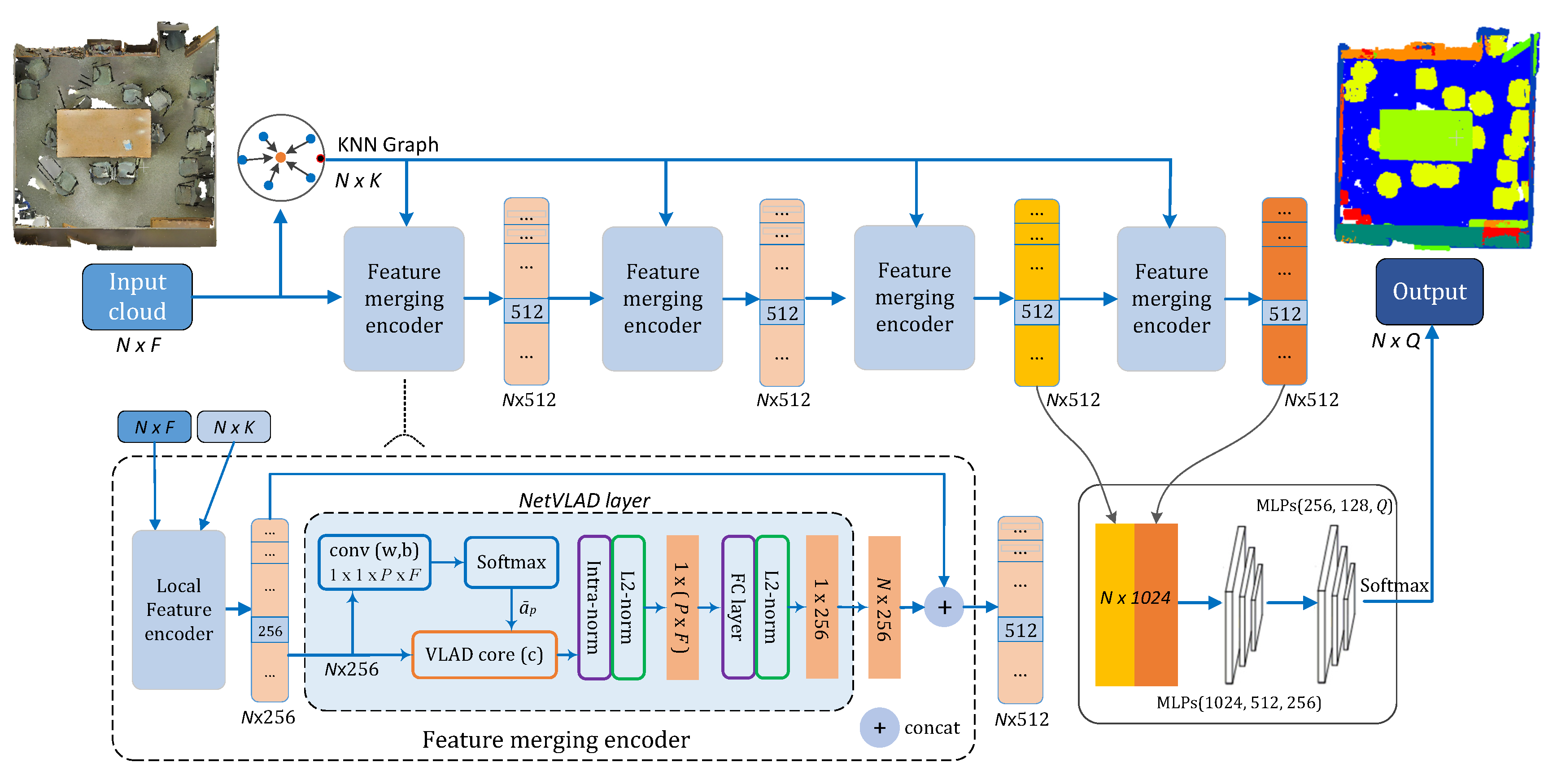
3.1. Knn Graph Convolution

For a point cloud with N points $X=\{x_1,x_2,\dots ,x_N\}\subseteq {\mathbb{R}}^F$, establish the KNN topological graph. As Figure 1 illustrates, the directional graph $\mathcal{G}=\{V,E\}$ shows the local structure of a point $x_i$ and its K nearest neighbors $\{x_{j_1},x_{j_2},\dots ,x_{j_k}\}$, in which $V=X$ and $E=$<$i,j_k$>, $x_i,x_{j_k}\in V$. Define edge feature $e_{ij}={\mathrm{h}}_{\theta }\{x_i,x_j\}$, in which ${\mathrm{h}}_{\theta }:{\mathbb{R}}^F\times {\mathbb{R}}^F\to {\mathbb{R}}^{F^{\prime }}$ is a nonlinear function with learning parameter $\theta$, and $F^{\prime }$ denotes the dimension of the edge features. Then, an aggregating operation $\mathcal{C}$ is applied on the K edge features to get the output $y_i$ corresponding to $x_i$, as defined in Equation (1).

$$y_i=\underset{j:(i,j)\in E}{\mathcal{C}}{\mathrm{h}}_{\theta }(x_i,x_j)$$

(1)

Figure 1. The illustration of K-Nearest Neighbor searching (KNN) graph convolution.

The choice of edge function and aggregation method is crucial to the proposed KNN graph convolution network. PointNet only encodes the global coordinates without considering the local structure, leading to unideal segmentation in local regions. To simultaneously take into account the global and local information, here we utilize an asymmetric operation as edge function:

$${\mathrm{h}}_{\theta }(x_i,x_j)={\mathrm{h}}_{\theta }(x_i,x_i-x_j)$$

(2)

The function obtains the global information through the query point $x_i$ and the local information through $(x_i-x_j)$. In this way, both the global and local features are counted to get stronger feature representation. For feature aggregation $\mathcal{C}$, we use the two-channel pooling (max and average pooling) techniques to compensate the information loss, retaining strong response and fine-grained local feature. To be specific, we define the following operator in Equation (3) to train edge feature, which could be considered as a shared MLP with learning parameters $\theta =\{\lambda ,\phi \}$ and activation function ReLU. Then, the aggregation can be realized on the edge features by Equation (4).

$$e_{ij}^{\prime }=\mathrm{ReLU}(\lambda ·x_i+\phi ·(x_i-x_j))$$

(3)

$$y_i^{\prime }=\underset{j:(i,j)\in E}{\max }{e}_{ij}^{\prime }+\underset{j:(i,j)\in E}{\mathrm{avg}}{e}_{ij}^{\prime }$$

(4)

3.2. Kgcn

To realize the above idea, we propose a KNN Graph Convolution Network (KGCN) consisting of three main parts, as shown in Figure 2.

Figure 2. The structure of the proposed KNN Graph Convolution Network (KGCN). Four local feature encoding blocks (big blue boxes, with detail structure shown in the dotted box) are assembled recursively to encode the local features, then the last two outputs (orange boxes) are concatenated for segmentation which labels the point cloud by two sets of MLPs. The four local feature encoding blocks follows the same design. The operation $\mathcal{L}$ (small green box) takes point features and the KNN graph and transforms them to a $N\times K\times 2F$ tensor which is trained by MLPs. Then, two pooling functions are applied and the responses are concatenated, followed by another MLP to generate $N\times 256$ local features.

-

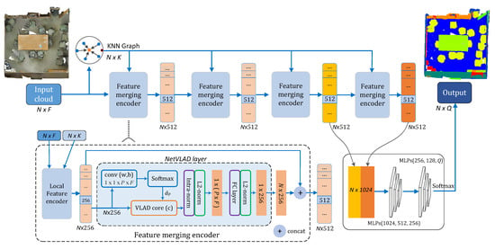
First, it searches the K nearest neighbors of each point and constructs the KNN graph ($N\times K$ tensor, N is the number of points) for the input point cloud ($N\times F$ tensor, here F represents the data dimension, usually including coordinates, colors, normals, etc.).

-

Afterward, the point cloud and its KNN graph are sent into the local feature encoder which transforms the inputs to a $N\times 256$ tensor. The local feature encoder block is recursively assembled for four times to expand the perception field, and each block could output different level of feature abstraction.

-

Finally, the third-level features and the final features are concatenated in the jump-connection style, followed by two sets of shared MLPs (MLPs $\{512,256,128\}$ and MLPs $\{128,64,Q\}$) for dimensionality reduction to get the semantic labels. The final output of the network is a $N\times P$ matrix, namely, the possibilities of each point belonging to P different categories, which can be further assigned by a softmax function.

As is implied in the network, the design of the local feature encoder plays a decisive role. As shown in Figure 2, the structure of the encoder basically follows the idea of KNN graph convolution introduced. First, the two input tensors—the point features and the K neighboring relations in ${\mathbb{R}}^F$ space—are merged and transformed to a $N\times K\times 2F$ tensor by a specific operation $\mathcal{L}$. Assume that $k_i$ stores the indices of the K nearest neighbors of point $x_i$ and $l_i$ signifies the transformed vector related to $x_i$, then the operation $\mathcal{L}$ is defined as

$$\begin{array}{cc}\hfill & \mathcal{L}:X\to L\end{array}$$

(5)

$$\begin{array}{cc}& L=\{l_1,\dots ,l_N\mid l_i\in {\mathbb{R}}^{K\times 2F}\}\end{array}$$

(6)

$$\begin{array}{cc}& l_i\left(j\right)=[x_i,x_i-x_j],j\in k_i\end{array}$$

(7)

Here, $l_i\left(j\right)$ corresponds to the neighbor $x_j$, and $[x_i,x_i-x_j]$ represents the concat of vector $x_i$ and $(x_i-x_j)$. The tensor of edge features is repressed as $E=\{e_1,\dots ,e_N\mid e_i\in {\mathbb{R}}^{K\times 128}\}$ which is computed by Equation (8):

$$e_i=\sigma \left(\mathcal{M}(\sigma \left(\mathcal{M}(l_i;{\theta }_1)\right);{\theta }_2)\right)$$

(8)

In this equation, $\mathcal{M}$ denotes a shared MLP and $\sigma$ means the activation function ReLU. ${\theta }_1$ and ${\theta }_2$ are, respectively, the learning parameter of the two MLPs. Afterward, the max-pooling and average-pooling are used in K channels to simultaneously get the strong and fine-grained responses. Then, the output features Y = $\{y_1,\dots ,y_N\mid y_i\in {\mathbb{R}}^{256}\}$ of the local feature encoder are determined by Equation (9), in which ${\theta }_3$ is the parameter of the last MLP. Cross-entropy function is employed to weigh the loss in the network training.

$$y_i=\sigma (\mathcal{M}([\underset{j\in k_i}{\max }\left(e_j\right),\underset{j\in k_i}{\mathrm{avg}}\left(e_j\right)];{\theta }_3))$$

(9)

3.3. Kvgcn

The KGCN extracts the global features via assembling local feature encoders repeatedly. This way it loses certain semantic contexts of scenes, causing confusions in dense or regions with similar appearance. To abstract and exploit the global contextual information effectively, we try to embed a Vector of Locally Aggregated Descriptors (VLAD) [22] layer into the proposed network and name it the KNN and VLAD combined Graph Convolution Network (KVGCN).

3.3.1. Overall Structure

VLAD is a traditional feature encoding algorithm based on feature descriptors, which is usually applied in image classification and instance retrieving. It is a technique that aggregates the local feature descriptors to global vectors with elaborate representation of local details but no data loss. Arandjelović et al. [37] simulated VLAD and designed a trainable generalized VLAD layer in the CNN framework, known as NetVLAD, to aggregate the local features. In this work, we embed the NetVLAD layer into our network and merge the local and global features for point cloud semantic segmentation (as shown in Figure 3).

Figure 3. The structure of the proposed KNN and VLAD combined Graph Convolution Network (KVGCN) which follows the encoder–decoder pipeline. Four feature merging encoders (blue boxes, with detail structure shown in the dotted box) are arrayed to merge the local and global features for representativeness. The point features and KNN graphs are taken as input by a local feature encoder. Then, the encoded $N\times 256$ local features are sent into the NetVLAD layer for global feature aggregation via a VLAD core followed by normalizations and concatenation. Similar to KGCN, two tensors are jump-connected for a decoding process to label the points.

The proposed KVGCN follows the similar encoder–decoder pipeline, whereas a new feature merging encoder is designed. The new feature encoder merges the $N\times 256$ local features and the global features aggregated by NetVLAD layer to compose the $N\times 512$ feature representation for the following decoding stage. The NetVLAD layer uses a convolution and a softmax function to compute parameters of the VLAD core which aggregates the input local features. Afterward, the L2-normalization and feature concatenation are introduced to generate the merged features. Similar to KGCN, two feature vectors from different stages are then jump-connected for a decoding process to label the points. For loss function, we follow the setting in KGCN and use the cross-entropy function to weigh the segmentation loss in network training.

3.3.2. Netvlad Layer

VLAD can be considered as a feature pooling method that stores the residuals of the feature vector and its cluster center. Given NF-dimensional local features $\left\{x_i\right\}$ as input, and P cluster centers $\left\{c_p\right\}$ as parameters, the output V of VLAD is a $P\times F$ representation matrix (Equation (10)) which is further normalized to a vector as the global feature. The ($j,p$) element of V is computed as

$$V(j,p)=\sum _{i=1}^N{a}_p\left(x_i\right)(x_i\left(j\right)-c_p\left(j\right))$$

(10)

where $x_i\left(j\right)$ and $c_p\left(j\right)$ are the jth element of the ith local feature and the pth cluster center. $a_p\left(x_i\right)$ defines the contribution of feature $x_i$ to cluster $c_p$; it is 1 or 0, meaning that $c_p$ is the closest cluster to $x_i$ or otherwise. Intuitively, the elements of matrix V records the residuals $(x_i-c_p)$ of each feature to each cluster. Apparently, VLAD is untrainable due to the discontinuity of $a_p\left(x_i\right)$.

In order to construct a trainable VLAD layer and embed it into a back-propagation network, the differentiability of the layer operation to its all parameters is required. To make the operation differentiable, the hard assignment of $a_p\left(x_i\right)$ is replaced with a soft assignment in Equation (11):

$${\overline{a}}_p\left(x_i\right)=\frac{e^{-\alpha {\parallel x_i-c_p\parallel }^2}}{{\sum }_{p^{\prime }}{e}^{-\alpha {\parallel x_i-c_{p^{\prime }}\parallel }^2}}$$

(11)

and ${\overline{a}}_p\left(x_i\right)$ ranges between 0 and 1 according to the proximity of feature $x_i$ to the cluster center $c_p$. Note that $\alpha$ is a positive parameter which controls the decay of the response and $\alpha \to +\infty$ corresponds to the original VLAD. This equation can be expanded and simplified by canceling $e^{-\alpha {\parallel x_i\parallel }^2}$ term, then we get a softmax function in Equation (12):

$${\overline{a}}_p\left(x_i\right)=\frac{e^{{\mathbf{w}}_p^T{x}_i+b_p}}{{\sum }_{p^{\prime }}{e}^{{\mathbf{w}}_{p^{\prime }}^T{x}_i+b_{p^{\prime }}}}$$

(12)

where ${\mathbf{w}}_p^T=2\alpha c_p$ and $b=-\alpha {\parallel c_p\parallel }^2$. Then, the soft-assignment of V is determined by Equation (13):

$$V(j,p)=\sum _{i=1}^N\frac{e^{{\mathbf{w}}_p^T{x}_i+b_p}}{{\sum }_{p^{\prime }}{e}^{{\mathbf{w}}_{p^{\prime }}^T{x}_i+b_{p^{\prime }}}}(x_i\left(j\right)-c_p\left(j\right))$$

(13)

$\left\{{\mathbf{w}}_p\right\}$,$\left\{b_p\right\}$ and $\left\{c_p\right\}$ are the trainable parameter sets of NetVLAD. Comparing to the original VLAD just having parameter set $\left\{c_p\right\}$, NetVLAD has three sets of parameters, enabling greater flexibility.

As shown in Figure 3, the NetVLAD layer includes three steps before the normalizations: (1) a convolution “conv($\mathbf{w},b$)” with P filters $\left\{{\mathbf{w}}_p\right\}$ of size $1\times 1$ and biases $\left\{b_p\right\}$, (2) the following “softmax” function which computes weight ${\overline{a}}_p\left(x_i\right)$ by Equation (12), and (3) the “VLAD core” taking ${\overline{a}}_p\left(x_i\right)$ as parameter to calculate the output matrix V by Equation (13). Afterward, the intra-normalization and L2-normalization are used to normalize the aggregated $P\times F$ features. A fully connected layer and L2-normalization are added to obtain the concise $1\times 256$ global descriptor, followed by a vector expansion operation to get the $N\times 256$ global features, which are then concatenated with local features for further processing.

3.4. Permutation Invariance

For unordered point cloud data, the premise of a model being invariant to input permutation is required. The local feature encoder uses two symmetric functions—max pooling and average pooling—to aggregate the information from each point, thus is invariant to input orders. Therefore, the NetVLAD layer also meets this requirement, meaning that it can be embedded to the feature merging encoder for point cloud feature learning.

The $1\times 1$ kernel only upsamples or downsamples the input feature without considering the spatial relations with others, so it will not be impacted by the input permutation, then we can get stable parameters from “conv($\mathbf{w},b$)” and “softmax” operations. Therefore, the invariance of NetVLAD to input permutation lies to that of the “VLAD core”.

Given N input feature descriptors $X=\{x_1,x_2,\dots ,x_N\}$ and the trained parameters of P clusters $\left\{{\mathbf{w}}_p\right\}$, $\left\{b_p\right\}$ and $\left\{c_p\right\}$, then the output of “VLAD core” is $V=\left[V\right(j,p\left)\right]$,

$$V(j,p)=\sum _{i=1}^N{\overline{a}}_p\left(x_i\right)(x_i\left(j\right)-c_p\left(j\right))=\sum _{i=1}^N{h}_{jp}\left(x_i\right)$$

(14)

$V(j,p)$ aggregates the residuals in the jth part of each descriptor to the pth cluster center. It is the sum of a function of descriptor $x_i$.

For another input, $\tilde{X}=\{x_i,x_1,\dots ,x_t,\dots ,x_N,x_{i+1}\}$ with the same descriptors as X but different input order, the corresponding “VLAD core” output $\tilde{V}=\left[\tilde{V}(j,p)\right]$ is calculated as

$$\tilde{V}(j,p)=h_{jp}\left(x_i\right)+h_{jp}\left(x_1\right)+\dots +h_{jp}\left(x_t\right)+\dots +h_{jp}\left(x_N\right)+h_{jp}\left(x_{i+1}\right)=\sum _{t=1}^N{h}_{jp}\left(x_t\right)$$

(15)

As the parameters are stable to input orders, the soft-assignment ${\overline{a}}_p\left(x_i\right)$ and the residual of the same descriptor remain stable, which means the Equations (14) and (15) represent the same output. Therefore, the “VLAD core” is invariance to input permutation, and so is the NetVLAD layer.

4. Experimental Results

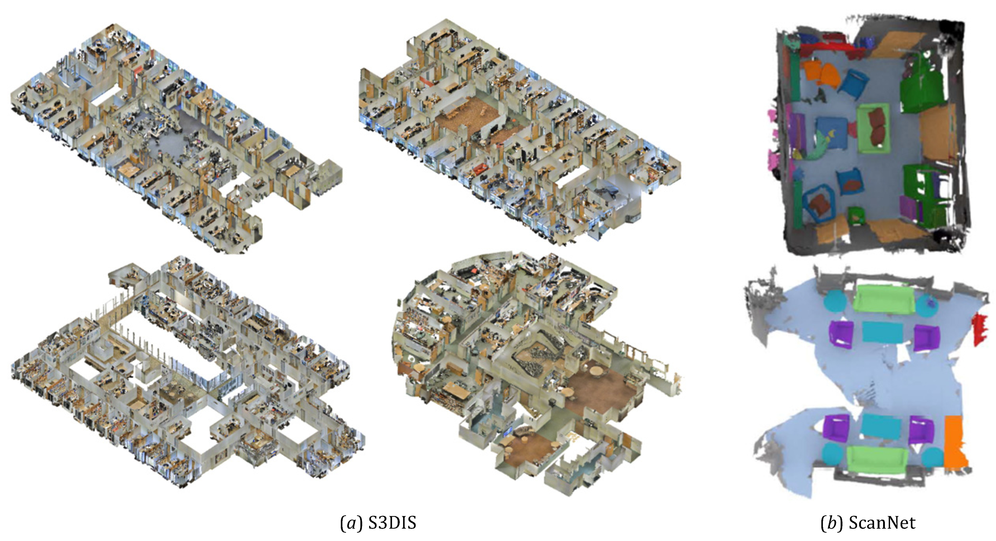
4.1. Datasets

To evaluate the performance of the proposed network, we test it on two different datasets: the high-density indoor datasets S3DIS [1] and ScanNet [38], as demonstrated in Figure 4.

Figure 4. Demonstration of the testing datasets. (a) S3DIS dataset. (b) ScanNet dataset.

S3DIS Dataset contains six different large-scale indoor scenes in three buildings, involving 11 room types, which are divided into 13 semantic categories. It covers an area of more than 6000 square meters, exceeding 200 million points that are composed of 3D coordinates, colors, and point labels. ScanNet is a dataset of richly annotated RGB-D scans of real-world environments containing 2.5 M RGB-D images in 1513 scans acquired in 707 distinct spaces, with estimated calibration parameters, camera poses, 3D surface reconstructions, textured meshes, and dense object-level semantic segmentations.

4.2. Experimental Details

As the S3DIS dataset is divided into six different areas, we follow the same evaluation protocol used in PointNet [11], which is a 6-fold cross-validation over all the areas, namely, choosing five areas as training set and one as testing set in each training and using cross-validation to establish six models to cover the whole dataset. Three widely used metrics—overall accuracy ($oAcc$), mean accuracy ($mAcc$), and mean intersection over union ($mIoU$)—are employed to measure the segmentation performances.

Each room in S3DIS dataset is divided into grids of 1 m × 1 m, and 4096 sample points are randomly collected in each grid. The entire room is then traversed in a step of 0.5 m. In the experiment, the number of sampled points is about 96.6 million, and each point is represented by a 9-dimension vector [$x,y,z,r,g,b,n_x,n_y,n_z$]. During the model training, the batch size 4096, the batch number for each training epoch is 12, and the number of training epoch is 100. For ScanNet, we follow the preprocessing settings in PointNet++ [12]. The point clouds are voxelized and divided into cubes of 1.5 m × 1.5 m × 3 m, and 8192 points with [$x,y,z$] coordinates are sampled from each cube. The 1201 samples out of total 1513 scanned scenes of ScanNet are used for training, and the other 312 samples are for testing. The training settings for S3DIS are copied.

4.3. Parameter Evaluations

Before conducting comparisons with state-of-the-art methods, we first evaluate the influence of two critical parameters on semantic segmentation to choose the best settings. The two parameters are the number of neighboring points K in KNN algorithm and the number of clusters D in NetVLAD layer. Our evaluations are carried out on S3DIS dataset, with “Area_5” as testing set and the other five areas as training set.

4.3.1. Parameter K

The parameter K controls the scope of neighbor searching and the volume of local information for training. Too small a value of K leads to inadequate local contextual information, and too large a value may include irrelevant noises and is computational expensive. The evaluation of K is performed by comparing the segmentation results of different settings in KGCN. Table 1 lists the segmentation metrics under six settings of K, and the trend can be observed though only six tests are carried out. It is easily concluded that the best setting is $K=20$ (highest $mAcc$, $mIoU$, and $oAcc$), and the segmentation accuracy does not improve with more neighboring information counted as usually anticipated. In the following evaluations, we fix parameter K to 20 for both KGCN and KVGCN.

Table 1. The segmentation accuracy (%) of KGCN on “Area_5” of S3DIS dataset for different K.

Metric	K = 5	K = 10	K = 15	K = 20	K = 25	K = 30
mAcc	52.4	59.6	62.8	63.5	63.2	60.3
mIoU	47.7	50.6	55.2	56.3	56.4	54.7
oAcc	74.6	79.5	81.8	83.2	82.5	79.6

4.3.2. Parameter D

In the NetVLAD layer of the proposed KVGCN, the input features are grouped to D clusters and then the output of “VLAD core” is calculated. This preset parameter D has a major impact on the performance of KVGCN. Here, we try to experimentally determine the optimal setting for D, and the segmentation results under different D are shown in Table 2. The segmentation accuracy arises with D ranges from 4 to 12 and drops afterwards. The optimal value cluster number is 12, which is also the setting for parameter D in the following evaluations.

Table 2. The segmentation accuracy (%) of KVGCN on “Area_5” of S3DIS dataset for different D.

Metric	D = 4	D = 8	D = 12	D = 16	D = 20	D = 24
mAcc	60.9	62.1	66.7	62.9	61.7	59.8
mIoU	54.7	57.6	59.3	56.3	54.4	51.1
oAcc	74.6	75.3	85.3	80.2	79.1	78.3

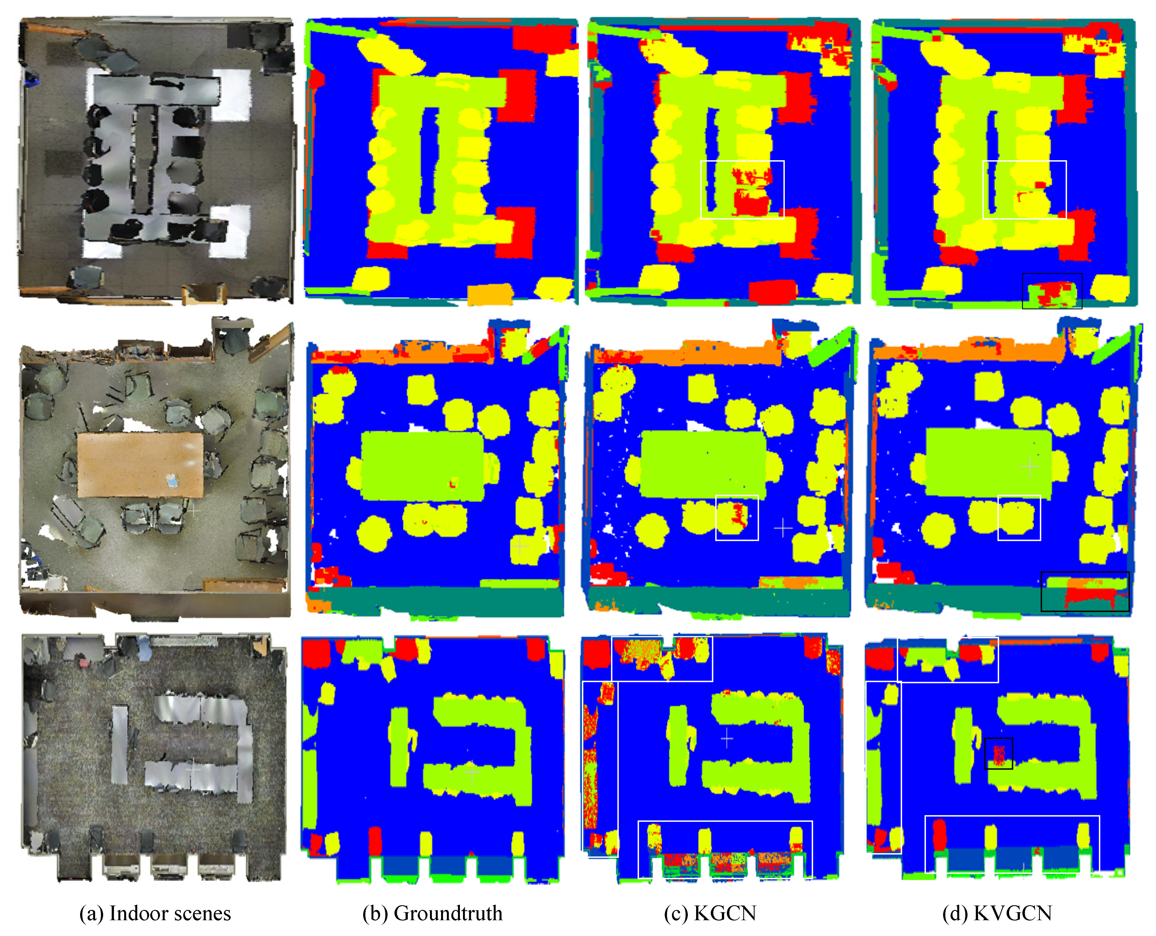
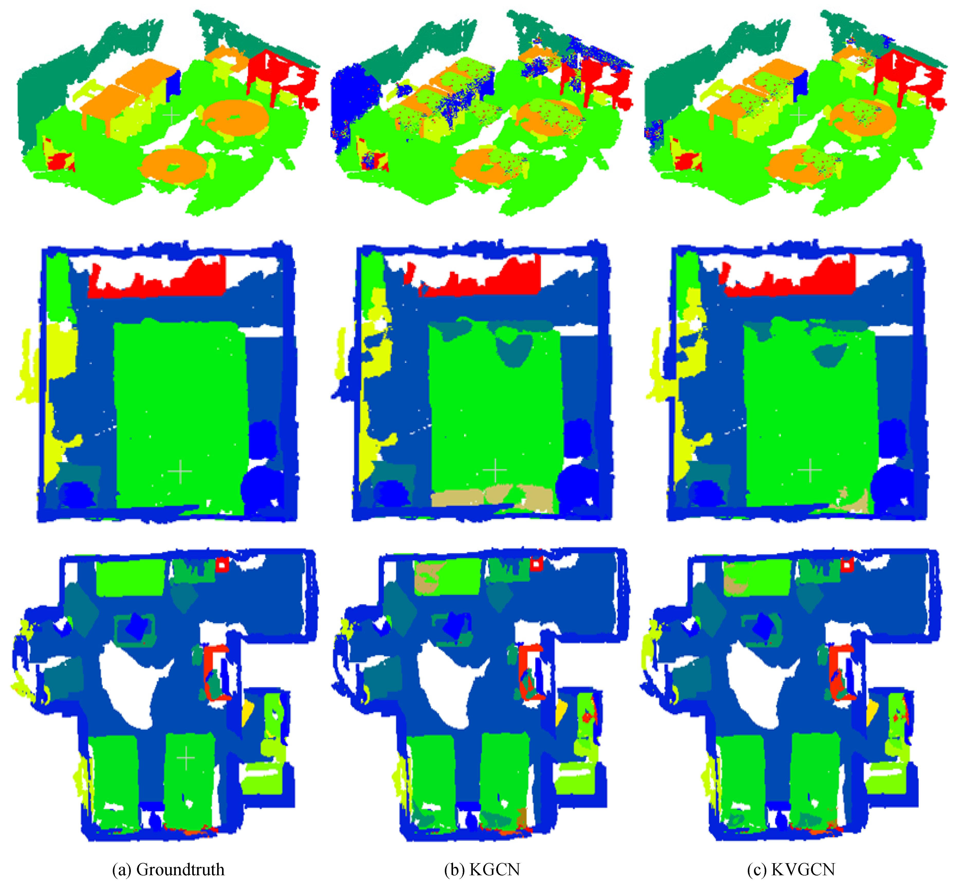
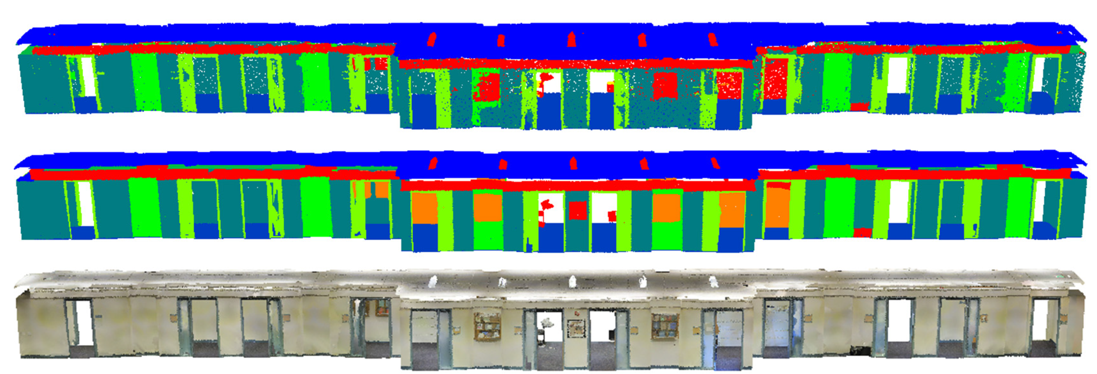
4.4. Comparison with Other Networks

4.4.1. S3dis Dataset

We gather the segmentation results of the proposed KGCN and KVGCN models on S3DIS dataset by 6-fold cross-validation and compare with state-of-the-art methods. The overall accuracy results are reported in Table 3, and the IoU scores of each semantic class are reported in Table 4. The mean IoU, overall accuracy, and mean accuracy of KGCN are, respectively, 59.0%, 85.8%, and 70.9%, which are better than PointNet [11], G+RCU [2], SEGCloud [3], RSNet [13], and A-SCN [19]. By combing the KNN and NetVLAD layer into the feature encoder, the KVGCN model further lifts the segmentation accuracy on S3DIS dataset, and the three metrics reach 60.9%, 87.4%, and 72.3%. Meanwhile, our KVGCN model improves the IoU results in five classes (Table 4). These quantitative results show that the NetVLAD is an essential feature pooling method for aggregating global features from local features and can promote the accuracy of point cloud semantic segmentation.

Table 3. Comparison of segmentation accuracy (%) on the entire S3DIS dataset.

Method	mIoU	oAcc	mAcc
PointNet [11]	41.1	78.5	49.0
G+RCU [2]	49.7	81.1	66.4
SEGCloud [3]	48.9	-	-
RSNet [13]	51.9	81.7	59.4
A-SCN [19]	52.7	81.6	-
KGCN	59.0	85.8	70.9
KVGCN	60.9	87.4	72.3

Table 4. IoU (%) of per semantic class in S3DIS dataset.

Method	Celling	Floor	Wall	Beam	Column	Window	Door	Chair	Table	Bookcase	Sofa	Board	Clutter
PointNet [11]	88.6	97.3	69.8	0.05	3.92	46.3	10.8	52.6	58.9	40.3	5.9	26.4	33.2
G+RCU [2]	90.3	92.1	67.9	44.7	24.2	52.3	51.2	58.1	41.9	6.9	47.4	39.0	30.0
SEGCloud [3]	90.1	96.1	69.9	0.0	18.4	38.4	23.1	78.6	70.4	58.4	40.9	13.0	41.1
RSNet [13]	92.5	92.8	78.6	32.8	34.4	51.6	68.1	60.1	59.7	50.2	16.4	44.9	52.0
SPGraph [33]	89.9	95.1	72.0	62.8	47.1	55.3	60.0	73.5	69.2	3.2	45.9	8.7	52.9
KGCN	94.3	93.5	78.4	52.5	35.0	53.7	62.9	64.4	62.0	20.4	51.5	42.0	50.2
KVGCN	94.5	94.1	79.5	53.4	36.3	56.8	63.2	67.5	64.3	23.6	54.3	43.1	53.2

To present intuitive observations, we select three samples to visualize the segmentation results, which are shown in Figure 5. KGCN segments most of the tables and chairs in the scenes, but the separation in certain parts (e.g., the chairs in the first two samples, denoted in white boxes) and the easily confused areas (e.g., the corner with several different objects and the conjunction parts of wall and windows in the third sample, denoted in white boxes) are ambiguous. Then, KVGCN aggregates the local and global contextual features and lifts the segmentation in these areas. Though better segmenting boundaries are obtained by KVGCN, there are few negative examples, which are marked by black boxes in the samples. Overall, KVGCN achieves comparative segmentation to groundtruth on S3DIS dataset.

Figure 5. Sample segmentation results of the S3DIS dataset. From left to right are the input scenes, groundtruth segmentation, and results by KGCN and KVGCN. KGCN outputs ambiguous segmentation in easily confused areas and KVGCN achieves better results, which are denoted by white boxes, while few negative examples are marked by black boxes.

4.4.2. Scannet Dataset

To evaluate the segmentation of the proposed models on the ScanNet dataset without color information, the 1201 samples out of total 1513 scanned scenes of ScanNet are used for training, and the other 312 samples are for testing. Table 5 gives the overall accuracy results, and Table 6 lists the IoU scores of each semantic class in the dataset. Results in Table 6 reveal that the KGCN outperforms PointNet [11], PointNet++ [12], and RsNet [13] in IoU of 11 categories (e.g., floor, chair, bathtub, bath curtain, etc.) and maintains comparative results for the other nine categories, meaning that the local feature encoders in KGCN can recognize and provide distinctive feature representations in local regions. Then, with the global aggregation layer NetVLAD combined in the feature encoder, KVGCN obtains richer semantic features to distinguish different objects. KVGCN promotes the segmentation IoUs of all classes in this dataset, including several challenging classes (such as sofa, sink, window, photo, etc.) and gains the best performance in 13 classes comparing to other methods. The overall results in Table 5 verify the advantages of KVGCN in three metrics $mIoU,oAcc,$ and $mAcc$.

Table 5. Comparison of segmentation accuracy (%) on the entire ScanNet dataset.

Method	mIoU	oAcc	mAcc
PointNet [11]	14.3	52.6	18.6
PointNet++ [12]	32.2	73.8	43.1
RSNet [13]	37.5	75.2	46.2
KGCN	38.7	80.7	48.3
KVGCN	40.4	82.3	49.4

Table 6. IoU (%) of per semantic class in ScanNet dataset.

Method	Wall	Floor	Chair	Table	Desk	Bed	Bookshelf	Sofa	Sink	Bathtub
PointNet [11]	68.3	86.6	35.4	31.8	1.42	19.3	2.7	30.6	0.3	0.4
PointNet++ [12]	72.1	88.3	60.3	44.7	10.9	48.6	49.1	49.3	28.3	40.3
RSNet [13]	78.4	90.5	61.3	49.9	34.4	51.5	50.3	53.3	32.4	45.6
KGCN	79.3	91.6	63.4	46.1	28.9	47.5	49.3	51.2	28.5	55.4
KVGCN	82.4	94.3	65.1	48.3	30.5	49.1	52.1	56.3	30.3	56.3
Method	Toilet	Curtain	Counter	Door	Window	Showercurtain	Refrigerator	Picture	Cabinet	Otherfurniture
PointNet [11]	0	0	4.3	0	0	0	0	0	3.7	0.2
PointNet++ [12]	29.8	31.8	19.5	25.5	3.6	1.8	17.6	0	21.7	1.8
RSNet [13]	53.6	5.8	21.8	27.5	7.3	2.8	36.5	0.6	29.7	17.6
KGCN	56.7	22.2	23.4	33.1	10.1	5.6	35.3	1.6	26.1	18.1
KVGCN	58.3	23.1	24.2	35.2	12.2	6.3	36.2	2.6	26.3	19.2

Intuitive examples are demonstrated in Figure 6. KGCN performs better in semantic parts with larger data portion, without causing so many mislabeled points comparing to existing methods. KVGCN gets closer segmentation to the groundtruth in semantic parts like chairs and walls, as well as in the easily confused regions, such as the joint parts between chair/desk and floor. KVGCN generates fewer mislabelings on the three examples. This illustrates that the proposed feature merging encoder in KVGCN is beneficial to aggregating meaningful global information and improves the semantic segmentation.

Figure 6. Sample segmentation results of the S3DIS dataset. From left to right are the input scenes, groundtruth segmentation, and results by KGCN and KVGCN. KVGCN generates less mislabelings.

5. Discussion

Establishing the local graph structure of the query point and convolving the graph edges to obtain powerful local features shows great advantage in feature representation. It can extract sophisticated features from graph structure compared with PointNet directly capturing single point’s feature, and causes less data loss in comparison to slicing in RNN. The choice of K in KNN graph construction plays a crucial role in the feature gathering. In this work, we employ a fix value for K, which could limit the ability of feature learning in dense area. An adaptive adjusting strategy for K or assuring uniform input points could be a plausible solution. The similar concern for parameter D in KVGCN also stands.

Another issue is that four feature encoders are assembled in the proposed KGCN and KVGCN for feature learning. As a general rule, a greater number of encoders implies a deeper network, meaning that more distinctive features could be learnt. However, too deep a network may result in gradient explosion or overfitting during network training. In this work, we determine to use four encoders based on experimental tests. Table 7 gives the segmentation performance of KGCN on “Area_5” of S3DIS using different number of local feature encoders. The segmenting metrics lift significantly when more encoders are used, especially from three to four, and start declining when more than four encoders are utilized. Therefore, we use four encoders in all evaluations of the proposed KGCN and KVGCN.

Table 7. The segmentation accuracy (%) of KGCN on “Area_5” of S3DIS dataset for different number of feature encoders assembled.

Encoders	2	3	4	5	6
mAcc	52.3	54.6	63.5	61.4	59.2
mIoU	47.1	50.6	56.3	53.2	51.7
oAcc	71.2	72.3	83.2	82.1	81.5

Assembling multiple local feature encoders does not guarantee that reliable global features could be trained. The segmentation of KGCN in object concentrated areas or easily confused areas is sub-average. To aggregate representative global vectors for making full use of the semantic information, the trainable version of VLAD, the NetVLAD layer, is introduced in our network. Similar to Fisher Vector [39] or other single-vector representations [40], NetVLAD considers each element of the local features and depicts fine-grained details without data loss. The most important characteristic of NetVLAD is that it is amenable to training via back-propagation, which make it pluggable into other deep learning architectures. By embedding NetVLAD, the proposed KVGCN significantly improved the segmentation performance. Figure 7 and Figure 8 illustrate more segmentation results of KVGCN. Comparing to the best network available [41], our network achieves comparative $oAcc$ and $mAcc$ results, but falls behind on the $mIoU$ metric. As a concrete manifestation, the separation in shapely similar areas, such as walls, embedded boards, objects in corners, etc., requires more distinguishable features in model training. However, NetVLAD has shown its potential power in feature aggregating; the study of exploiting and enhancing NetVLAD for global feature aggregation could be a promising future direction.

Figure 7. More segmentation samples of the proposed KVGCN method. The KVGCN result and the groundtruth segmentation are pairwise illustrated. Upper: segmented results by KVGCN. Lower: groundtruth.

Figure 8. Another large sample of segmentation results of the proposed KVGCN method. From top to bottom are the KVGCN result, groundtruth segmentation, and the actual scene of hallway.

6. Conclusions

This work designs a new graph convolutional network architecture that is trained for semantic segmentation of point cloud data in an end-to-end manner. The input points and KNN graph topological information are sent into four orderly assembled feature encoders to train powerful features for semantic segmentation. The encoder performs edge convolution on each query point and its nearest K neighbors to gain rich details, outperforming existing methods that only focus on isolated points. Another highlight is that we introduce the powerful pooling mechanism with learnable parameters that can be easily trained via back-propagation, NetVLAD layer, in the proposed feature merging encoder to aggregate global representation from local features. This combination of KNN graph and NetVLAD layer pays off on the final segmentation. We evaluated the proposed network on two challenging indoor datasets, and the results show its superiority in segmentation (better $mIoU$, $oAcc$, and $mAcc$). Based on this work, further research could focus on designing a network with adjustable parameters and high training efficiency.

References

1. Armeni, I.; Sener, O.; Zamir, A.R.; Jiang, H.; Brilakis, I.; Fischer, M.; Savarese, S. 3d semantic parsing of large-scale indoor spaces. In Proceedings of the IEEE Conference on Computer Vision and Pattern Recognition (CVPR), Las Vegas, NV, USA, 27–30 June 2016; pp. 1534–1543. [Google Scholar]
2. Engelmann, F.; Kontogianni, T.; Hermans, A.; Leibe, B. Exploring spatial context for 3d semantic segmentation of point clouds. In Proceedings of the IEEE International Conference on Computer Vision (ICCV), Venice, Italy, 22–29 October 2017; pp. 716–724. [Google Scholar]
3. Tchapmi, L.; Choy, C.; Armeni, I.; Gwak, J.; Savarese, S. Segcloud: Semantic segmentation of 3d pointclouds. In Proceedings of the 2017 International Conference on 3D Vision (3DV), Qingdao, China, 10–12 October 2017; pp. 537–547. [Google Scholar]
4. Su, H.; Maji, S.; Kalogerakis, E.; Learned-Miller, E. Multi-view convolutional neural networks for 3d shape recognition. In Proceedings of the IEEE International Conference on Computer Vision (ICCV), Santiago, Chile, 7–13 December 2015; pp. 945–953. [Google Scholar]
5. Maturana, D.; Scherer, S. Voxnet: A 3d convolutional neural network for real-time object recognition. In Proceedings of the 2015 IEEE RSJ International Conference on Intelligent Robots and Systems (IROS), Hamburg, Germany, 28 September–2 October 2015; pp. 922–928. [Google Scholar]
6. Kalogerakis, E.; Averkiou, M.; Maji, S.; Chaudhuri, S. 3D shape segmentation with projective convolutional networks. In Proceedings of the IEEE Conference on Computer Vision and Pattern Recognition (CVPR), Honolulu, HI, USA, 21–26 July 2017; pp. 3779–3788. [Google Scholar]
7. Le, T.; Bui, G.; Duan, Y. A multi-view recurrent neural network for 3D mesh segmentation. Comput. Graph. 2017, 66, 103–112. [Google Scholar] [CrossRef]
8. Wu, Z.; Song, S.; Khosla, A.; Yu, F.; Zhang, L.; Tang, X.; Xiao, J. 3d shapenets: A deep representation for volumetric shapes. In Proceedings of the IEEE Conference on Computer Vision and Pattern Recognition (CVPR), Boston, MA, USA, 7–12 June 2015; pp. 1912–1920. [Google Scholar]
9. Qi, C.R.; Su, H.; Niessner, M.; Dai, A.; Yan, M.; Guibas, L.J. Volumetric and Multi-view CNNs for Object Classification on 3D Data. In Proceedings of the IEEE Conference on Computer Vision and Pattern Recognition (CVPR), Las Vegas, NV, USA, 27–30 June 2016; pp. 5648–5656. [Google Scholar]
10. Shi, B.; Bai, S.; Zhou, Z.; Bai, X. Deeppano: Deep panoramic representation for 3-d shape recognition. IEEE Signal Process. Lett. 2015, 22, 2339–2343. [Google Scholar] [CrossRef]
11. Qi, C.R.; Su, H.; Mo, K.; Guibas, L.J. PointNet: Deep learning on point sets for 3d classification and segmentation. In Proceedings of the IEEE Conference on Computer Vision and Pattern Recognition (CVPR), Honolulu, HI, USA, 21–26 July 2017; pp. 652–660. [Google Scholar]
12. Qi, C.R.; Yi, L.; Su, H.; Guibas, L.J. Pointnet++: Deep hierarchical feature learning on point sets in a metric space. arXiv 2017, arXiv:1706.02413. [Google Scholar]
13. Huang, Q.; Wang, W.; Neumann, U. Recurrent slice networks for 3d segmentation of point clouds. In Proceedings of the IEEE Conference on Computer Vision and Pattern Recognition (CVPR), Salt Lake City, UT, USA, 18–23 June 2018; pp. 2626–2635. [Google Scholar]
14. Scarselli, F.; Gori, M.; Tsoi, A.C.; Hagenbuchner, M.; Monfardini, G. The graph neural network model. IEEE Trans. Neural Netw. 2009, 20, 61–80. [Google Scholar] [CrossRef] [PubMed]
15. Xu, M.X.; Dai, W.R.; Shen, Y.M.; Xiong, H.K. MSGCNN: Multi-scale Graph Convolutional Neural Network for Point Cloud Segmentation. In Proceedings of the Fifth IEEE International Conference on Multimedia Big Data, Singapore, 11–13 September 2019; pp. 118–127. [Google Scholar]
16. Mao, J.G.; Wang, X.G.; Li, H.S. Interpolated Convolutional Networks for 3D Point Cloud Understanding. In Proceedings of the IEEE International Conference on Computer Vision (ICCV), Seoul, Korea, 27 October–2 November 2019; pp. 1578–1587. [Google Scholar] [CrossRef]
17. Thomas, H.; Qi, C.R.; Deschaud, J.; Marcotegui, B.; Goulette, F.; Guibas, L. KPConv: Flexible and Deformable Convolution for Point Clouds. In Proceedings of the 2019 IEEE CVF International Conference on Computer Vision (ICCV), Seoul, Korea, 27–28 October 2019; pp. 6410–6419. [Google Scholar] [CrossRef]
18. Li, Y.; Bu, R.; Sun, M.; Wu, W.; Di, X.; Chen, B. PointCNN: Convolution On X-Transformed Points. arXiv 2018, arXiv:1801.07791. [Google Scholar]
19. Xie, S.; Liu, S.; Chen, Z.; Tu, Z. Attentional shapecontextnet for point cloud recognition. In Proceedings of the IEEE Conferenceon Computer Vision and Pattern Recognition (CVRP), Salt Lake City, UT, USA, 18–22 June 2018; pp. 4606–4615. [Google Scholar]
20. Komarichev, A.; Zhong, Z.C.; Hua, J. A-CNN: Annularly Convolutional Neural Networks on Point Clouds. In Proceedings of the IEEE Conference on Computer Vision and Pattern Recognition (CVRP), Long Beach, CA, USA, 16–20 June 2019; pp. 7421–7430. [Google Scholar]
21. Bello, S.A.; Yu, S.; Wang, C.; Adam, J.M.; Li, J. Review: Deep Learning on 3D Point Clouds. Remote Sens. 2020, 12, 1729. [Google Scholar] [CrossRef]
22. Jégou, H.; Douze, M.; Schmid, C.; Pérez, P. Aggregating local descriptors into a compact image representation. In Proceedings of the 2010 IEEE Computer Society Conference on Computer Vision and Pattern Recognition, San Francisco, CA, USA, 13–18 June 2010; pp. 3304–3311. [Google Scholar] [CrossRef]
23. Huang, J.; You, S.Y. Pole-like object detection and classification from urban point clouds. In Proceedings of the IEEE International Conference on Robotics and Automation (ICRA), Seattle, WA, USA, 26–30 May 2015; pp. 3032–3038. [Google Scholar]
24. Pang, G.; Neumann, U. Fast and Robust Multi-view 3D Object Recognition in Point Clouds. In Proceedings of the International Conference on 3D Vision, Lyon, France, 19–22 October 2015; pp. 171–179. [Google Scholar]
25. Pang, G.; Neumann, U. 3D point cloud object detection with multi-view convolutional neural network. In Proceedings of the IEEE International Conference on Robotics and Automation (ICRA), Stockholm, Sweden, 16–21 May 2016; pp. 585–590. [Google Scholar]
26. Qiu, R.Q.; Neumann, U. Exemplar-Based 3D Shape Segmentation in Point Clouds. In Proceedings of the International Conference on 3D Vision, Stanford, CA, USA, 25–28 October 2016; pp. 203–211. [Google Scholar]
27. Liu, W.; Wang, Z.; Liu, X.; Zeng, N.; Liu, Y.; Alsaadi, F.E. A survey of deep neural network architectures and their applications. Neurocomputing 2017, 234, 11–26. [Google Scholar] [CrossRef]
28. Klokov, R.; Lempitsky, V. Escape from cells: Deep kd-networks for the recognition of 3d point cloud models. In Proceedings of the IEEE International Conference on Computer Vision (ICCV), Venice, Italy, 22–29 October 2017; pp. 863–872. [Google Scholar]
29. Riegler, G.; Osman, U.A.; Geiger, A. Octnet: Learning deep 3d representations at high resolutions. In Proceedings of the IEEE Conference on Computer Vision and Pattern Recognition (CVPR), Honolulu, HI, USA, 21–26 July 2017; pp. 3577–3586. [Google Scholar]
30. Liang, Z.D.; Yang, M.; Deng, L.Y.; Wang, C.X.; Wang, B. Hirarchical Depthwise Graph Convolutional Neural Network for 3D Semantic Segmentation of Point Clouds. In Proceedings of the International Conference on Robotics and Automation(ICRA), Montreal, QC, Canada, 20–24 May 2019; pp. 8152–8158. [Google Scholar]
31. Wang, Y.; Sun, Y.B.; Liu, Z.W.; Sarma, S.E.; Bronstein, M.M.; Solomon, J.M. Dynamic Graph CNN for Learning on Point Clouds. ACM Trans. Graph (TOG) 2019, 38, 146. [Google Scholar] [CrossRef]
32. Xie, Z.Y.; Chen, J.Z.; Peng, B. Point clouds learning with attention-based graph convolution networks. Neurocomputing 2020, 402, 245–255. [Google Scholar] [CrossRef]
33. Landrieu, L.; Simonovsky, M. Large-scale pointcloud semantic segmentation with superpointgraphs. In Proceedings of the IEEE Conferenceon Computer Vision and Pattern Recognition (CVRP), Salt Lake City, UT, USA, 18–23 June 2018; pp. 4558–4567. [Google Scholar]
34. Hu, Z.; Zhen, M.; Bai, X.; Fu, H.; Tai, C.L. JSENet: Joint semantic segmentation and edge detection network for 3d point clouds. In Proceedings of the European Conference on Computer Vision (ECCV), Glasgow, UK, 23–28 August 2020. [Google Scholar]
35. Mazur, K.; Lempitsky, V. Cloud Transformers. 2020. Available online: https://arxiv.org/pdf/2007.11679v2.pdf (accessed on 2 March 2021).
36. Zhao, H.; Jiang, L.; Jia, J.; Torr, P.; Koltun, V. Point Transformer. Available online: https://arxiv.org/pdf/2012.09164v1.pdf (accessed on 2 March 2021).
37. Arandjelović, R.; Gronat, P.; Torii, A.; Pajdla, T.; Sivic, J. NetVLAD: CNN Architecture for Weakly Supervised Place Recognition. IEEE Trans. Pattern Anal. Mach. Intell. 2018, 40, 1437–1451. [Google Scholar] [CrossRef] [PubMed]
38. Lin, H.; Chen, H.; Dou, Q.; Wang, L.; Qin, J.; Heng, P. Scannet: A fast and dense scanning framework for metastatic breast cancer detection from whole-slide images. In Proceedings of the 2018 IEEE Winter Conference on Applications of Computer Vision (WACV), Lake Tahoe, NV, USA, 12–15 March 2018; pp. 539–546. [Google Scholar] [CrossRef]
39. Perronnin, F.; Liu, Y.; Sanchez, J.; Poirier, H. Large-scale image retrieval with compressed Fisher vectors. In Proceedings of the 2010 IEEE Conference on Computer Vision and Pattern Recognition (CVPR), San Francisco, CA, USA, 13–18 June 2010; pp. 3384–3391. [Google Scholar] [CrossRef]
40. Philbin, J.; Chum, O.; Isard, M.; Sivic, J.; Zisserman, A. Object retrieval with large vocabularies and fast spatial matching. In Proceedings of the 2007 IEEE Conference on Computer Vision and Pattern Recognition, Minneapolis, MN, USA, 17–22 June 2007; pp. 1–8. [Google Scholar] [CrossRef]
41. Semantic Segmentation on S3DIS. Available online: https://paperswithcode.com/sota/semantic-segmentation-on-s3dis (accessed on 2 March 2021).
Publisher’s Note: MDPI stays neutral with regard to jurisdictional claims in published maps and institutional affiliations.
Article Metrics
Citations
Article Access Statistics
Multiple requests from the same IP address are counted as one view.