Article

Scene Complexity: A New Perspective on Understanding the Scene Semantics of Remote Sensing and Designing Image-Adaptive Convolutional Neural Networks

1
School of Geosciences and Info-Physics, Central South University, Changsha 410083, China
2
Institute of Technology Innovation, Hefei Institutes of Physical Science, Chinese Academy of Sciences, Hefei 230088, China
3
School of Tourism and Geography, Yunnan Normal University, Kunming 650500, China
4
GIS Technology Research Center of Resource and Environment in Western China of Ministry of Education, Kunming 650500, China
5
School of Information Science and Technology, Yunnan Normal University, Kunming 650500, China
*
Author to whom correspondence should be addressed.
Remote Sens. 2021, 13(4), 742; https://doi.org/10.3390/rs13040742
Submission received: 19 January 2021 / Revised: 7 February 2021 / Accepted: 12 February 2021 / Published: 17 February 2021

Abstract

:
Scene understanding of remote sensing images is of great significance in various applications. Its fundamental problem is how to construct representative features. Various convolutional neural network architectures have been proposed for automatically learning features from images. However, is the current way of configuring the same architecture to learn all the data while ignoring the differences between images the right one? It seems to be contrary to our intuition: it is clear that some images are easier to recognize, and some are harder to recognize. This problem is the gap between the characteristics of the images and the learning features corresponding to specific network structures. Unfortunately, the literature so far lacks an analysis of the two. In this paper, we explore this problem from three aspects: we first build a visual-based evaluation pipeline of scene complexity to characterize the intrinsic differences between images; then, we analyze the relationship between semantic concepts and feature representations, i.e., the scalability and hierarchy of features which the essential elements in CNNs of different architectures, for remote sensing scenes of different complexity; thirdly, we introduce CAM, a visualization method that explains feature learning within neural networks, to analyze the relationship between scenes with different complexity and semantic feature representations. The experimental results show that a complex scene would need deeper and multi-scale features, whereas a simpler scene would need lower and single-scale features. Besides, the complex scene concept is more dependent on the joint semantic representation of multiple objects. Furthermore, we propose the framework of scene complexity prediction for an image and utilize it to design a depth and scale-adaptive model. It achieves higher performance but with fewer parameters than the original model, demonstrating the potential significance of scene complexity.

Graphical Abstract

1. Introduction

Scene understanding is one of the essential and challenging tasks for computer vision and photogrammetry [1]. It plays a vital role in many applications, such as autonomous driving, navigation, indoor and outdoor mapping, as well as localization [2,3]. In particular, the classification task is the basis for some downstream tasks, such as segmentation [4] and detection [5]. Its Key is acquiring strong representative features to represent the semantic knowledge of images. Thanks to the rapid development of research related to convolutional neural networks [6,7,8], the automatic learning of features from images now replaces the manual construction of features in the past. In recent years, the focus of research has gradually shifted from designing sophisticated feature extraction algorithms [9,10,11,12,13] to building efficient network architecture [14] to learn expressive features. Some works focus on introducing prior knowledge into the architecture of networks to improve the learning of features. Studies [15,16] try to combine satellite image characters and the general convolutional neural network. Chen et al. [17] proposed a CNN architecture by combining a scene’s context to perform object detection. Qu et al. [18] presented a modified Faster-RCNN to solve the problem of object detection in infrared streetscape images with limited samples. Liu et al. [19] designed a superpixel-guided embedding CNN to handle limited labeled data and irregular spatial dependency in remote sensing images. Moreover, Xu et al. [20] proposed a segmentation model that uses guided filters to rectify the features. These works focus on improving performance by modifying the architecture of networks based on artificial prior knowledge.
Many methods [21,22,23] for scene recognition of remote sensing images have been proposed in recent years, but these methods use the same network for all images. Is this the right way? It is counter-intuitive: some scenes are easier to recognize, while others are harder to recognize. In other words, using a uniform architecture or introducing artificial priors while ignoring the differences in the images themselves may cause a mismatch in feature learning, e.g., in Figure 1, commercial center and dense residential are similar in content, it requires the network to learn the feature of the style. The reason behind this is the gap between the inherent nature of the images and the features learned by the network architecture. However, current research lacks an analysis of the relationship between the two.
Bridging the gap between image properties and feature learning of network faces three problems:
  • how to measure the inherent properties of images.
  • how to analyze the relationship between image properties and features learned from different structures.
  • how to make the features learned within the network correspond to the semantic concepts of images for straightforward interpretation.
For the first problem, although some methods, e.g., cosine similarity and Euclidean distance, reflect the differences between images, they lack the characterization of the images themselves. Structural similarity assesses the variability among statistical features between images but lacks semantic features. We introduce scene complexity to measure the intrinsic property of images. It considers high-level semantic feature representations and image memorability to evaluate one scene concept’s learning difficulty more objectively. Several scene complexity measurements have been proposed, such as radiosity and scene visibility complexity [24], which applied the concept of entropy from information theory to study 3D scene visibility. Methods introduce the cognitive neuroscience to discuss potential image properties, such as saliency [25,26], memorability [27] and search difficulty [28]. Some studies use it in feature matching to help improve object tracking [29]. Nevertheless, there is little literature about the synthesis of human visual perception and computer vision. In this paper, we decompose the estimation into two components: the memorability and search difficulty of an image. Specifically, we proposed a pipeline for scene complexity evaluation using visual processing tasks and building a scene complexity dataset called the AID-22. It is the first scene complexity dataset in remote sensing, and its images are mainly sampled from the AID [30]. For the second problem, Remote sensing images are sensitive to scale and are hierarchical in semantic representation. We analyze the relationship between the nature of images and the scale and hierarchy of features. Since the scale and hierarchy in CNNs are mainly determined by the size of receptive field and depth in the network architecture, which is the fundamental element of the network architecture, we analyze the relationship between images of various complexity and the depth and receptive field of the network. For the third problem, some works tried to open the black box of CNNs to interpret the mechanism of feature learning. Some works focus on visualizing the activation neurons [31] or the inverse mapping of the max response on neurons [32]. These works demonstrate that CNNs learn features, from general features to high-level semantic features, layer by layer. Furthermore, Zhou et al. [33] proposed CAM to automatically learn the contribution of image region features to the semantic representation. Therefore, we use CAM to visualize the mapping relationship between attention in learning features and scene objects at different complexity levels.
The contributions of our work are as follows:
  • We introduce scene complexity and analyze the relationship between remote sensing scenes of different complexity and the scale and hierarchy of feature learning in CNNs.
  • We propose a scene complexity measure that integrates scene search difficulty and scene memorability. Besides, we construct the first scene complexity dataset in remote sensing.
  • We design a scene complexity prediction framework to adapt different complexity data to the network depth and scale, which effectively improves the downstream model’s recognition accuracy and reduces the number of parameters.
  • We visualized and analyzed the relationship between semantic concept representation and model feature learning for scenes of different complexity, showing that complex scenes rely on learning multi-object features jointly to support semantic representation.

2. Materials and Methods

2.1. The Scene Complexity Dataset Construction

The quality of the training dataset is an important factor that impacts the performance of a model [34]. Considering the nature of scene complexity, we select 22 categories of scenes, whose complexity is more distinguishable, from the AID dataset [30] as our basic dataset because of its applicable characteristics. The dataset contains 360 samples per class; each sample is a 600 × 600 pixels RGB image with a spatial resolution ranged from 1 to 8m. Note that to balance the image size with the hardware limits, we resize the original images to 256 × 256 pixels in the experiments.
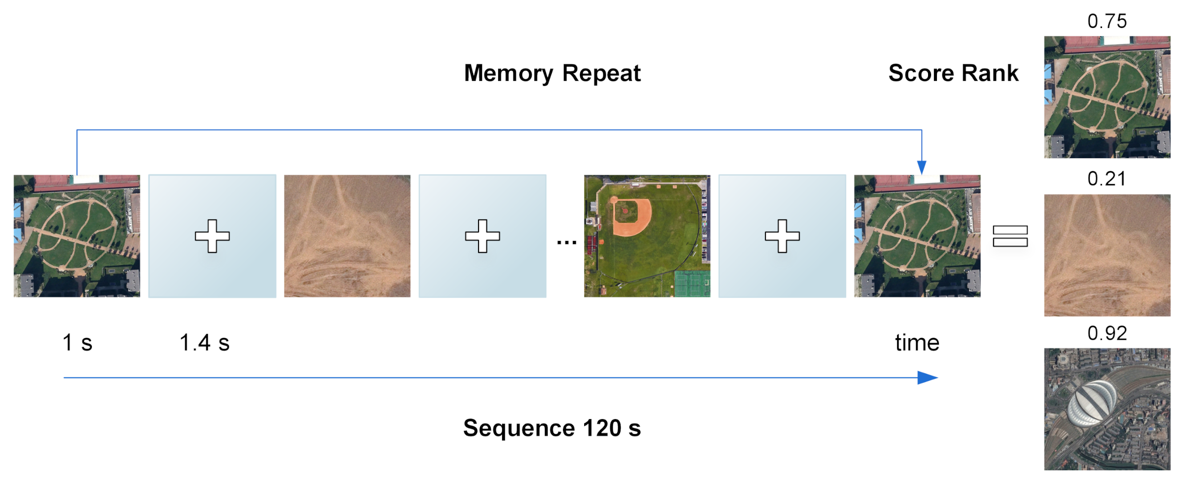
Evaluating the degree of the images is central to building our dataset. Referring to how humans understand diverse complex scenes, the more complicated a scene is, the more difficult it is to search for objects that belong to the scene, and memorizing it is even more difficult. Based on this cognitive phenomenon, we addressed the problem by measuring how memorable an image is and how easily it can be searched. We refer to [27] that characterized the consistency of an image memory across various observers and time delays. To measure image memorability, we asked volunteers to view a sequence of images. During the process, they would scan each image for 1 s and have 1.4 s rest. Once they recognized an image they had seen before, they would report the image. We shuffled images and asked volunteers to rest before the next sequence (we set a time of 12 s for the sequence) to avoid exhaustion (the procedure is shown in Figure 2). We asked volunteers to repeatedly view the images and then recognize them and rank them according to the length of repeated sessions required to recognize them. The longer the repeated session, the higher the memorability score. The pictures were then scored for memorability (from 1 to 10) based on the repeated session times. Moreover, the scores were normalized to 0 to 1.
Similar to [28], we tested the human response time during the visual search task and converted it into difficulty scores. We invited volunteers to select 10 to 15 samples randomly and asked them to execute the following visual tasks:
  • Given an image they were required to answer “yes” or “no” to a question about whether there was a particular object class in the image or point to a location when asked to locate a randomly selected object in the image, for example,” Is there an airplane?” or “Where is the house?”;
  • The response time to correctly answer the questions about the image was recorded;
  • For each image, the average response time for the two types of question, across all the volunteers, was calculated;
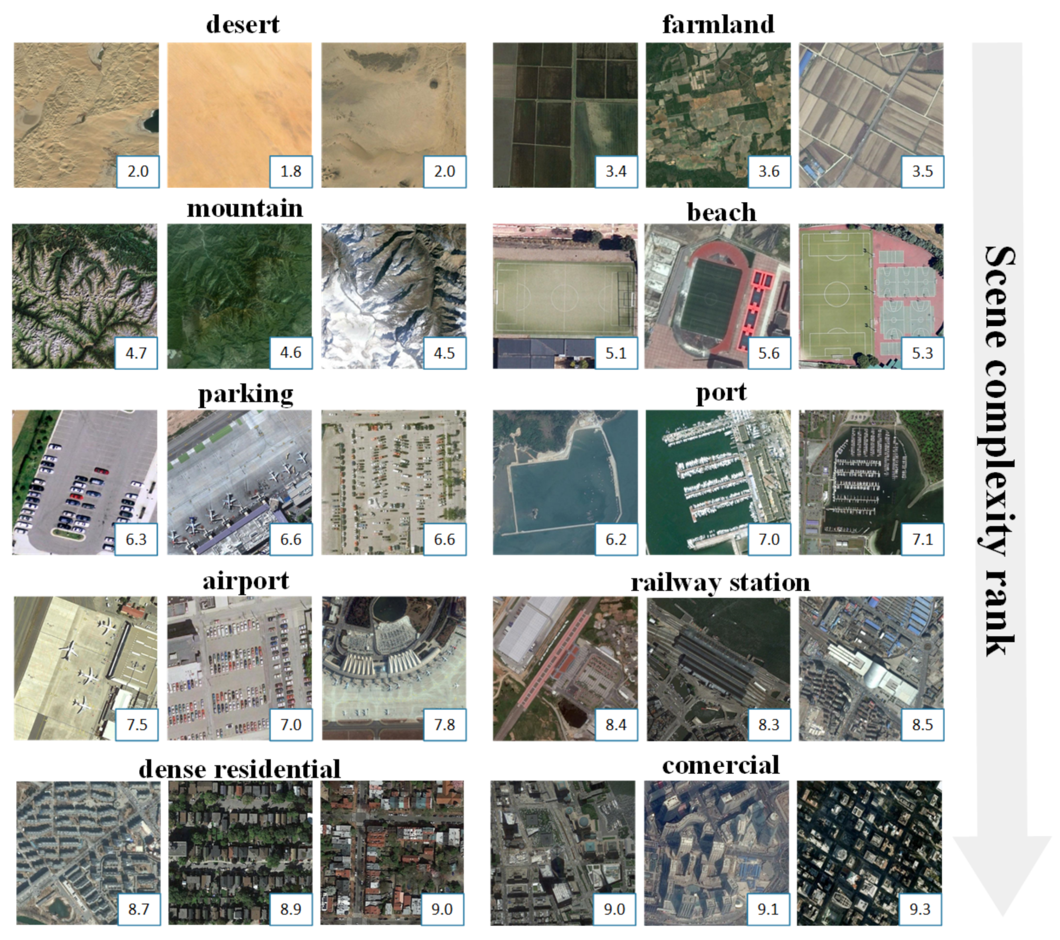
  • The sum of the search difficulty score and the memorability score is used as the scene complexity score of an image (Figure 3).
To simplify the experiment, we normalized an image’s score on the range 1 to 10 and divided the range into three superclasses: low, middle, and high complexity. Furthermore, we calculated the mean of a category’s complexity scores as the total score and used the K-means clustering method, setting K = 3 , to automatically categorize the dataset into three clusters. Figure 4 shows the three levels of the clustering result. The number in the circle indicates the clustering center, and the elements surrounding it shows the mean score of each category.

2.2. Methods

2.2.1. How to Control the Scale of Learning Feature

The scale of feature learning is mainly decided by two factors: the input image’s size and the receptive fields (RFs). Because we usually use uniform input size in one network, we mainly discuss the receptive fields in this paper. The depth and kernel size control the scope of receptive fields. To control the variables, we use the same depth and only adjust the kernel size in convolutional layers to explore the effect of the features’ scale on the recognition of scenes of different complexity. Specifically, we train the GoogLeNet [35], which is composed of multiple inceptions. The original inception V1 contains two layers: the first layer is three parallel convolutional layers with kernel size 1 × 1 and one pooling layer; the second layer is three parallel convolutional layers with various kernel size 1 × 1, 3 × 3, and 5 × 5, which ensure to learning multiple scales of features. Besides it, we modify three versions of inception based on it as a contrast. Figure 5 shows the architecture of the modified inception with RFs, which indicate the scale of features.

2.2.2. How to Control the Hierarchy of Learning Feature

Deep network extracts high-level semantic features via stacked layers [6], which ensure the feature can encode a scene’s concept. To explore the hierarchy of feature learning in remote sensing imagery understanding, we train models with various depth, which ensures the feature is of multiple levels of features, from scene complexity.
To analyze the influence of network depth on remote sensing scene recognition, we trained models using the VGG-16/19 models [36], which are composed of 13 or 16 convolution layers and three fully connected layers. Both of the networks utilize a uniform convolutional kernel size of (k = 3 × 3 ), which eliminates the interference of other possible factors. We implemented the experiments in the Caffe [37] and trained models on the AID-22. The capacity of networks is sufficient for classifying this dataset [38], which avoids the interference of network capacity change to experimental results.

2.2.3. Designing Image-Adaptive Networks with Scene Complexity

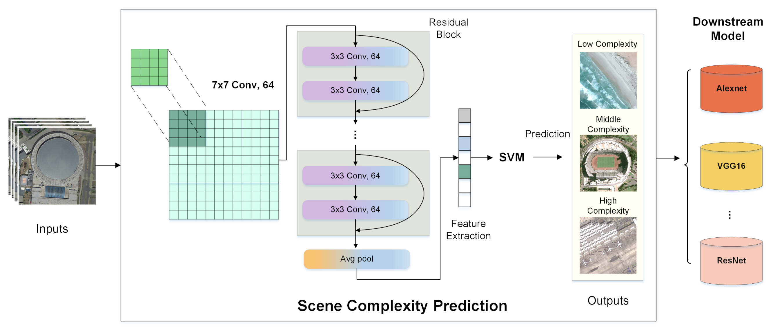
Predicting the degree of scene complexity. Benefiting from the strong capabilities of CNN for feature representation, we view scene complexity as synthesizing multiple-levels of features. We use resnet-18 [39] rather than other classic models to extract features of one scene because it is easy to train and can learn better features. In Figure 6, we show the pipeline of scene complexity prediction. It contains three steps: firstly, we train the pretrained resnet-18 on the constructed scene complexity dataset. The resnet-18 is trained 100,000 iterations with an initial learning rate lr = 1 × 10⁻³, batch size = 64. Secondly, we use it to extract the features of the last FC-layer. Thirdly, we utilize the extracted features to train the SVM to predict the scene complexity of images. The categories of images are sorted into three degrees of complexity by the prediction score. It achieves 92.85% test accuracy on complexity prediction. This result suggests that classifying the scene complexity is a high-level semantic task, and deep convolution neural networks can do well.
Improving the recognition accuracy and lighten the model parameters size. The prediction of complexity plays the role of data preprocessing. It categories the images with complexity and take them into the downstream networks with various depth (e.g., revised VGG-16). We designed modified versions of VGG-16. Table 1 shows the architectures of VGG-16*. Compared with the original VGG-16, all use the same convolutional layers, except that fully connected layers and output layers (VGG-16*-A) for different scene complexity images are configured behind different convolutional layers, respectively, thus allowing images of different complexity to adapt to different network depths. All images share the shallow layer of the network. Moreover, the number of neurons in the output layer is modified because the number of processed scene classes decreases much, and the fully connected layer no longer needs such a massive number of neurons. Considering the massive number of flatten layer parameters corresponding to low and medium complexity, we use Maxpool and Global average pool (GAP) and process them parallel, i.e., Maxpool processes the convolutional layer’s information inputs it to the next convolutional layer. In contrast, GAP processes the convolutional layer’s information and flows to each output module (VGG-16*-D). In addition to significantly reducing the number of parameters in the model, GAP integrates global information, while using global information in the shallow layers is sufficient. We also give two other versions (VGG-16*-B, VGG-16*-D) depending on the GAP modules’ location.

2.2.4. Class Activation Mapping and Semantic Representation

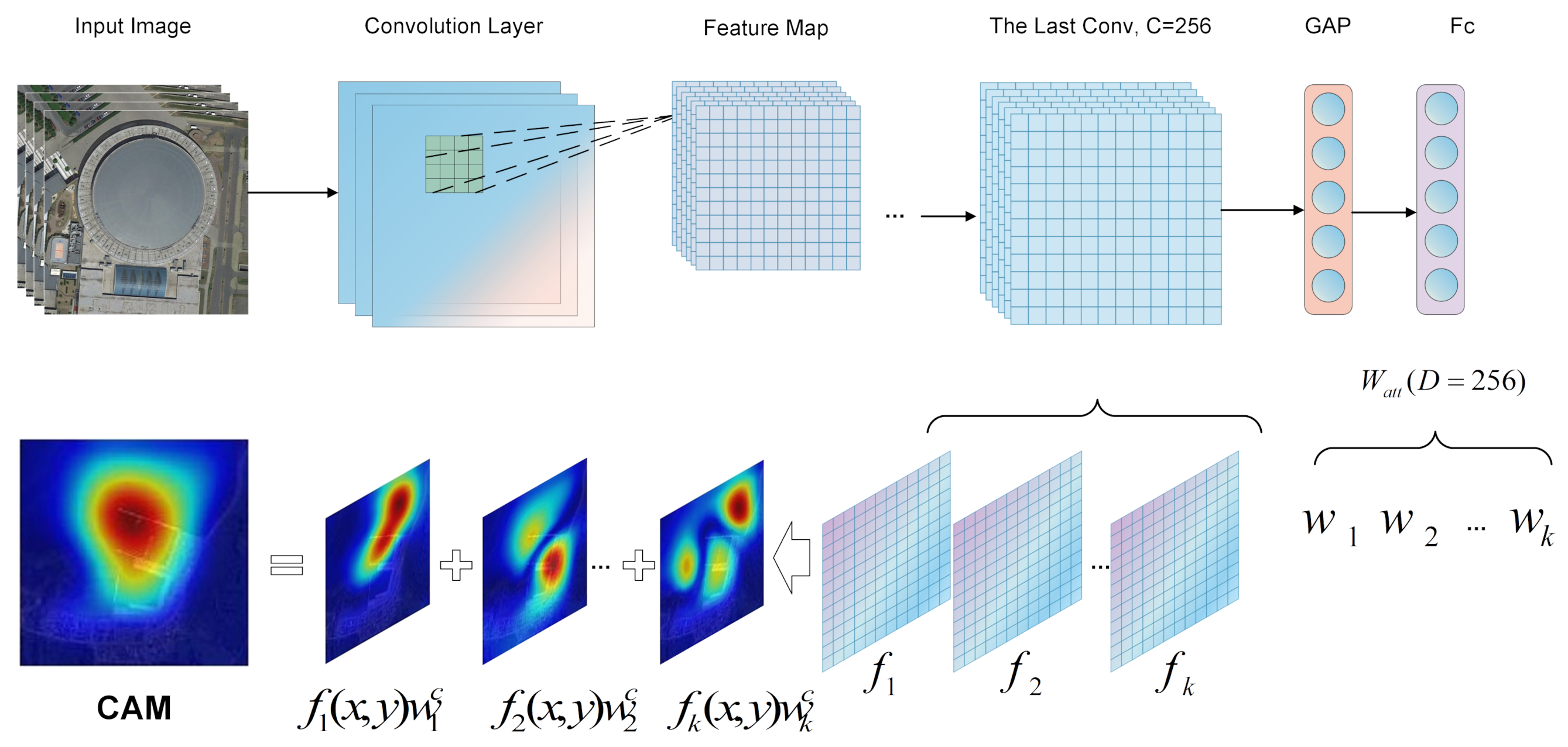
To explore the feature learning mechanism for images of different complexity, we utilized a visual approach named Class Activation Mapping (CAM) [33] to map the relationship between the output and the original input image. It visualizes the pixels that highly contribute to recognition. CAM learns the mapping from the pixels of an image to the output probability and reflects the weights that pixels contribute to the prediction score via a heat map (Figure 7). The most important part is building the class activation maps, it is calculated by:
M c = K w k c f k ( x , y )
where k is the number of neurons in the last convolution layer, w k c is the weight that the k-th neuron contributes to the prediction score corresponding to class c, and f k ( x , y ) is the activation function of the k-th neuron of the last convolution layer at position (x, y). To calculate the feature maps’ weight in the last convolutional layer, the full connected layer of GoogLeNet, which is between the last convolution layer and the output layer, is replaced with global average pooling (GAP) and the auxiliary loss function is removed.

2.3. Training Details

We train all models on our constructed scene complexity dataset. It contains 3 degrees of complexity, a total of 22 categories, each class of 360 samples. Furthermore, the dataset is divided into the training set, validation set, and test set in a ratio of 3:1:1. We implemented models on Caffe. In all experiments, we initialize the models’ weights using a Gaussian distribution. The activation function used is the ReLU activation function. We use a grid search to obtain the best model by setting the learning rate as η = 0.1 , 0.01 , 0.001 , 0.0001 , and divide it by 10 per 50,000 iterations. The maximum number of iterations is 300,000. The optimization policy is stochastic gradient descent with a batch size equal to the maximum number of examples that the hardware could support. We test models every 10,000 iterations and then save the best result as the final model. The momentum is 0.9, and the weight decay is 0.0005. We resize the input image to the size networks required and train models using the NVIDIA GTX1070 8GB GPU.

3. Results

Current studies [40] prove that a model learns a scene by encoding objects’ distribution. However, the feature representation that the model learns remains unclear. Thus, we explored the relationship among the semantic concept of a scene, the scale, and the hierarchy of feature learning, based on CNN’s, from the perspective of scene complexity. Our experiments use our own constructed AID-22 scene complexity dataset, which contains three degrees of scene complexity image samples. Moreover, as introduced in Section 2, these sample complexities are clustered to obtain the corresponding complexity degree. Furthermore, we constructed an adaptive network to improve model performance based on VGG-16. It can adjust its depth and scales to the scene complexity of an image. The experimental results show that the modified network increases the recognition accuracy with only one-tenth parameters.

3.1. How the Scale of Feature Learning Influences the Recognition of Scenes with Different Complexity

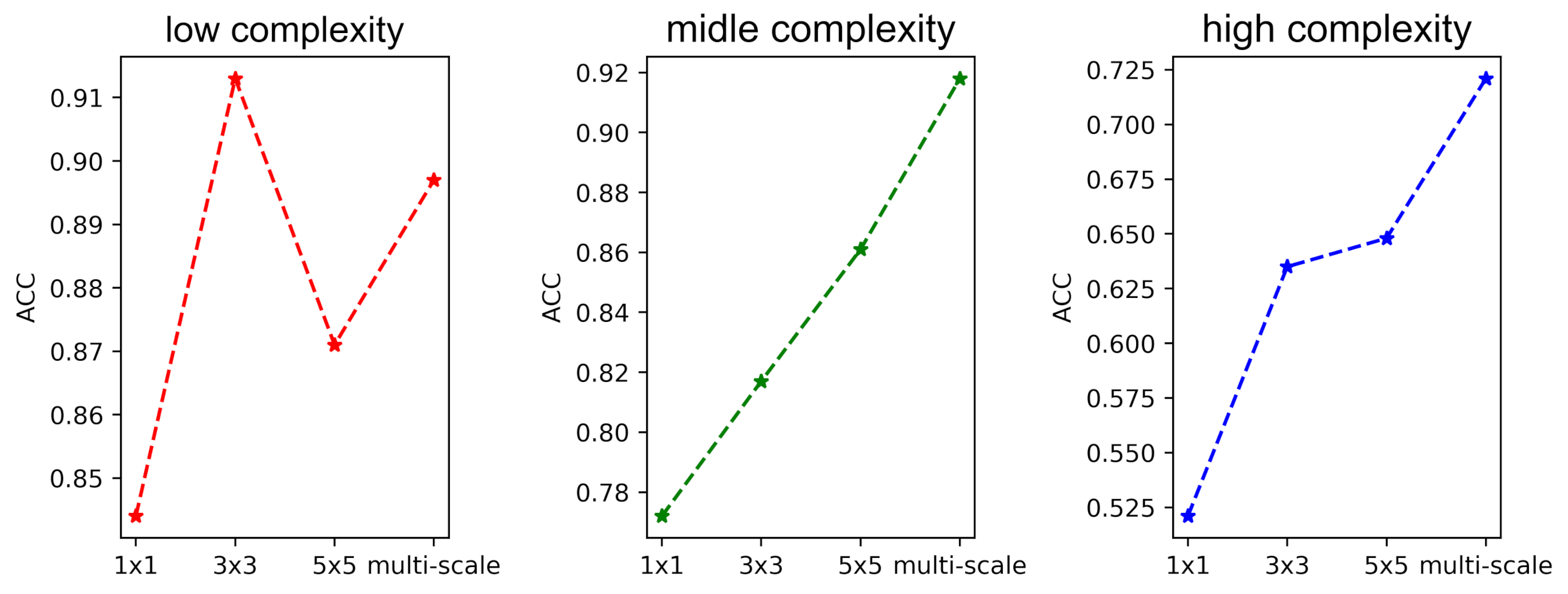
Except for the overall accuracy (OA), which is defined by the ratio of the predicted sample to the entire data sample, we utilize the kappa coefficients [41] to evaluate the performance of the model because it measures the consistency between the prediction and ground truth more objectively. Experimental results show that RFs significantly influence remote sensing scene recognition. Multiple scale features are usually useful for improving the overall accuracy in scene recognition. Table 2 shows that the kappa coefficient of GoogLeNet with multiple scales RFs is higher than that of other single-scale RF models. The inception 5 × 5 model, with a larger convolution kernel scale, works best in single-scale RF models; the smallest scale inception, 1 × 1, drops more than others. It suggests that the different levels of granularity of features have various weights for the whole dataset.
To explore the relationship between RFs and scene complexity, we separately analyzed category recognition accuracy with complexity. With increasing scene complexity, the model with a multi-scale RFs performs better than the single-scale architecture. As seen in Figure 8, the four inception models have nearly the same performance in the low scene complexity categories, but it is evident that the multi-scale inception works best.
The classes with high scene complexity are sensitive to the change of the learning feature’s scale, while classes with low scene complexity are not sensitive. As shown in Figure 9, the precision curve rises as the scale increases. Note that the multi-scale model rises the fastest and that a similar phenomenon occurs with moderate-complexity scene recognition, but it is not evident in low-complexity scenes. It indicates that a complicated scene representation requires multiple-scale features. Nonetheless, it is sufficient to encode simple scenes with single-scale features.

3.2. How the Hierarchy of Feature Learning Influences the Recognition of Scenes with Different Complexity

Experimental results in Table 3 show that a deeper network performs better on overall accuracy. The VGG-19 model achieves higher accuracy than the VGG-16 model. And the overall accuracy of the VGG models, with the best performance of is 95%. While the GoogLeNet, which is lower than VGG, has 83% OA (Table 2). It suggests that a deeper network is usually beneficial for improving the overall recognition but may lead to higher computational costs and time complexity.
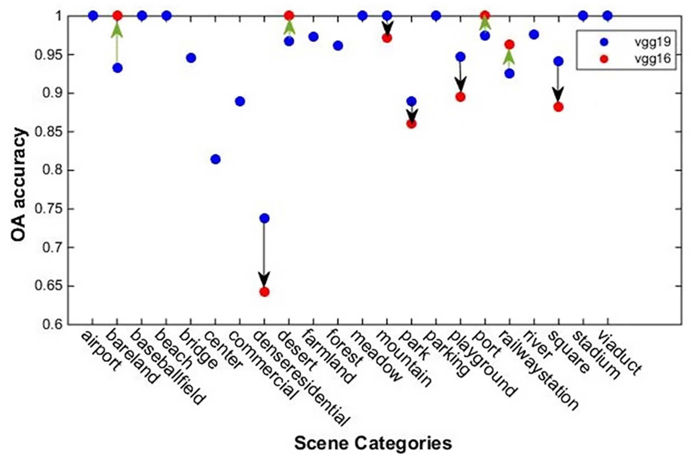
We further investigated different classes’ recognition and found that different depth models are good at identifying different scenes. As seen in Figure 10, the VGG-16 is preferable for bare land recognition and has weak performance in the mountain category, whereas the VGG-19 model performs better than the VGG-16 model in recognizing the playground. It shows that different scenes require a specific depth of networks. Thus, we conclude that a unified depth of features may benefit partial categories of scenes but may obstruct some scenes’ recognition.
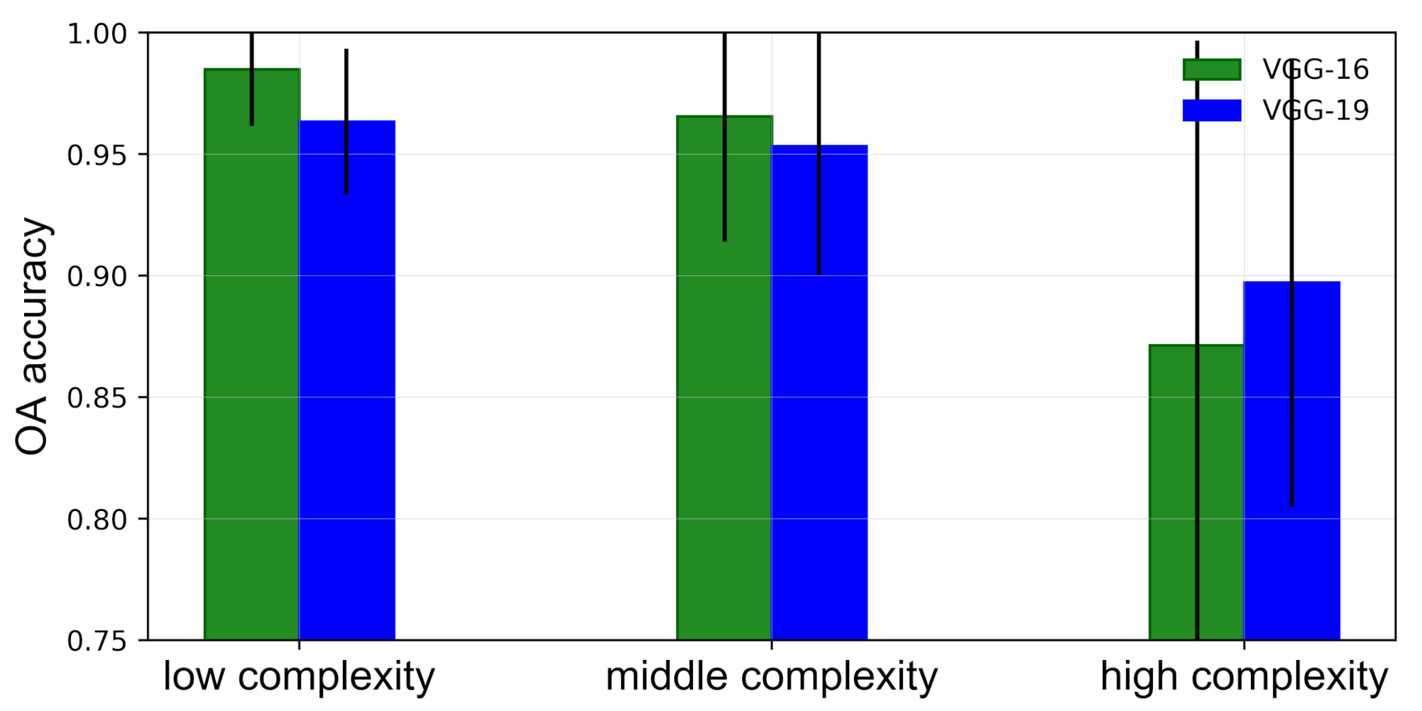
We calculated the overall average accuracy of images with different scene complexity on various deep networks in Figure 11. Simple scenes are more easily recognized on shallow networks, while complex sets rely more on deep networks. Deeper network models can significantly improve the recognition accuracy of complex networks but may impair simple scenes’ recognition. Specifically, when using VGG-19, the OA accuracy improves by 3% on highly complex sets; however, the OA accuracy decreases on all other complexity scenes, especially on simple sets. We also calculate the standard deviation of recognition accuracy for each complexity scene, as shown by the solid black line. We find that the recognition accuracy of the shallow network is more stable on the low complexity scene. In contrast, the recognition accuracy of the deep network is more stable on the high complexity scene. Thus, we can conclude that the complex scene relies more on the high-level features, while the simple scene relies more on the shallow features. Under such conditions, the recognition accuracy of models is higher and more stable.
More precisely, because the Kendall correlation coefficient is constant in the range of the various measurements, we utilized it to compute the correlation between the VGG-Net depth variable and the change in the samples’ probability from the VGG-16 model to the VGG-19 model. The Kendall π is 0.179, which indicates that a complex scene is sensitive to network depth and that a positive correlation exists between the scene complexity and network depth. We speculate that the Kendall value would increase for a more complex dataset or for some models that have much larger differences in network depth because some of the categories, especially ones with high-complexity scenes, are recognized as well.

3.3. How Adaptive Networks Based on Scene Complexity Improve Model’s Performance

According to the above analysis, different complexity requires matching features of different scales and depths. Specifically, simple scenes rely on shallow and global single-scale feature learning, while complex sets rely on deep and multi-scale feature learning. How to build adaptive networks for images of specific complexity? Based on VGG-16, we construct the depth adaptive ground VGG-16* (Table 1) to verify how scene complexity helps the model learn features better and improve its performance. Table 4 shows the comparison results between the VGG-16* family and the plain VGG-16. The deep adaptive ground network(without GAP) improves 0.4% in test accuracy and 1.5% in training accuracy. It increases the number of network parameters by 1.5 times and requires longer training time. Furthermore, VGG-16*-B/C/D reduces the number of model parameters and training time after using GAP. And the recognition accuracy has been further improved.
Moreover, when we configure GAP for all output layer modules, the number of VGG-16*-D’s parameters is reduced by 9 times, and the accuracy is improved by nearly 0.8%—noting that it is not advantageous to use GAP on all complexity images. The model’s recognition accuracy can be enhanced when using GAP on simple scenes (VGG-16*-B/C), but the recognition accuracy decreases when using GAP on complex sets (VGG-16*-D). It is mainly because the GAP operation preserves global information but ignores local details, which are crucial in the semantic representation of high complexity scenes. To summarize, by using scene complexity adaptive models, it is possible to improve the accuracy by almost 2%, reduce the model parameters by nearly 9 times, and reduce the training time by twice. We conclude that adaptive networks based on the scene complexity can effectively improve the performance of scene recognition.

4. Discussion

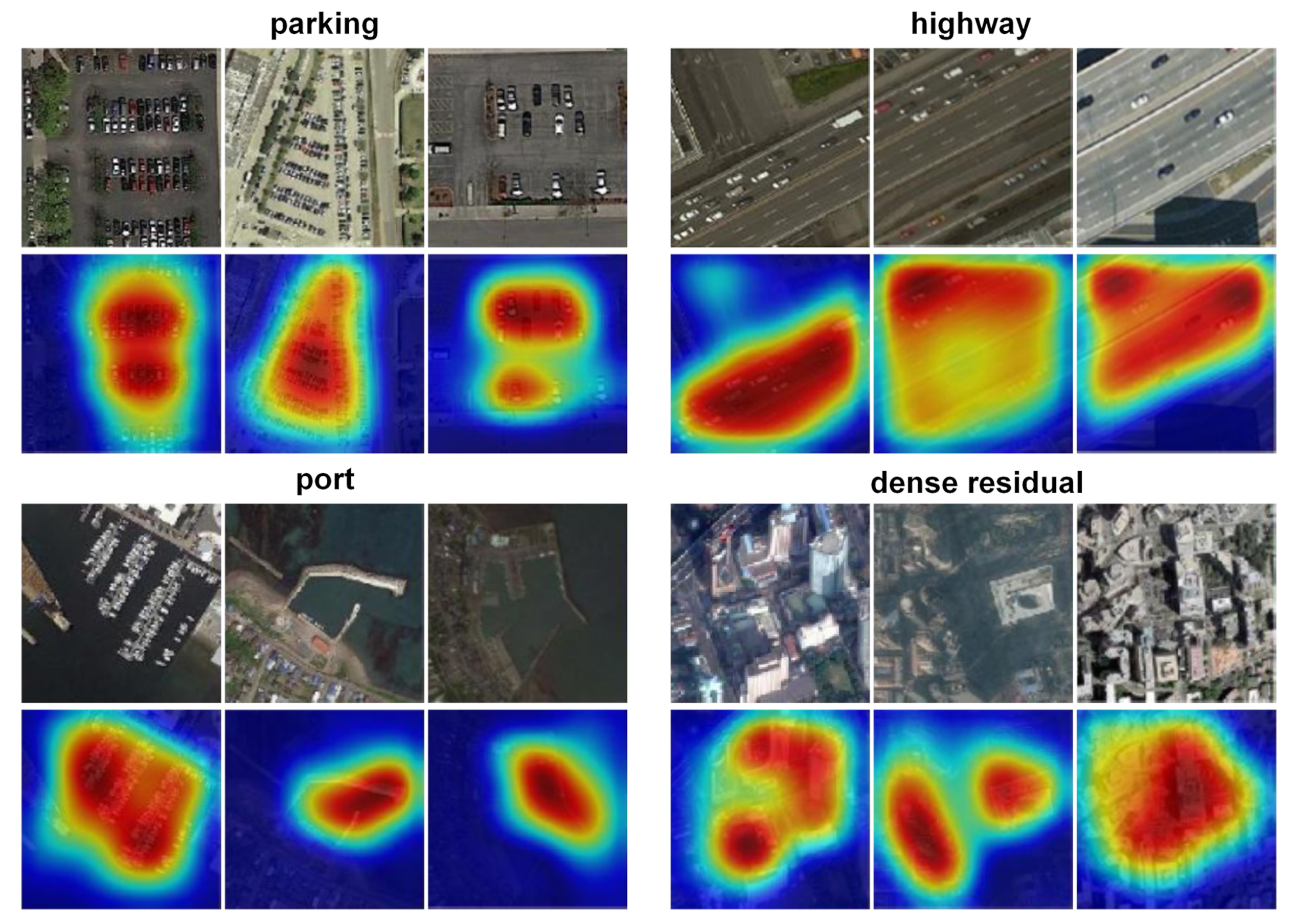
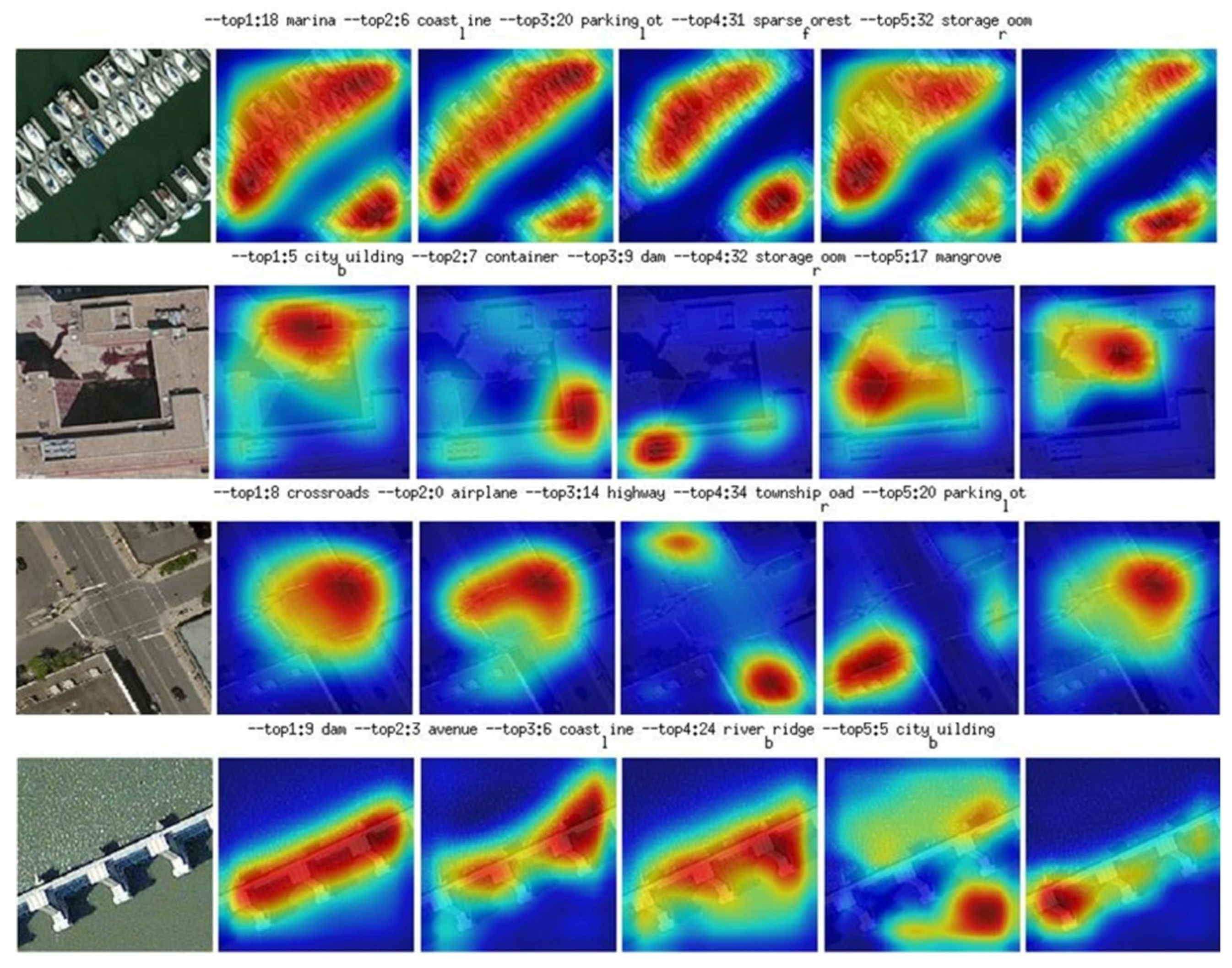
We explored the influence of feature learning on scene recognition by analyzing the learned features’ distribution patterns. As introduced in Section 2, we use CAMs to visualize the mapping of learned features to the input image, quantifying the contribution of different regions in the image to the semantic concept representation. CAMs are obtained by training GoogLeNet*, with a recognition accuracy of 91.82%, ensuring that the learned features are representative. The experimental results show that the scene semantic concept relies on the encoding of multiple objects and their distribution patterns. In Figure 12, vehicles are highlighted, which indicates that cars and their combined distribution patterns are critical to represent the concept of parking. Simultaneously, the highway class relies on the encoding of vehicles’ features in addition to the characteristics of roads, and the two together encode the semantic concept representation of highways. A similar phenomenon occurs in other scenarios. For instance, in the port class, CAMs respond only to boats and their distribution, and dense residuals respond only to buildings.
Analyzing the relationship between feature learning and the corresponding prediction via CAMs, the experiments indicate that learning objects’ pattern dramatically influences the prediction result. Figure 13 shows the most likely categories of an image. When the model learns the sea, sand, and waves’ features, it recognizes the beach as “beach”. However, if the model ignores sand features’ learning, it acknowledges the beach as a “port”. This method offers a way to dissect critical parts of the model from the perspective of feature learning. Moreover, We list some of the CAMs in Figure 14, which are categories of the RSI-CB [42], to demonstrate it is independent of specific datasets. We trained GoogLeNet* to generate CAMs and resized the hot maps to the same size as the input images.
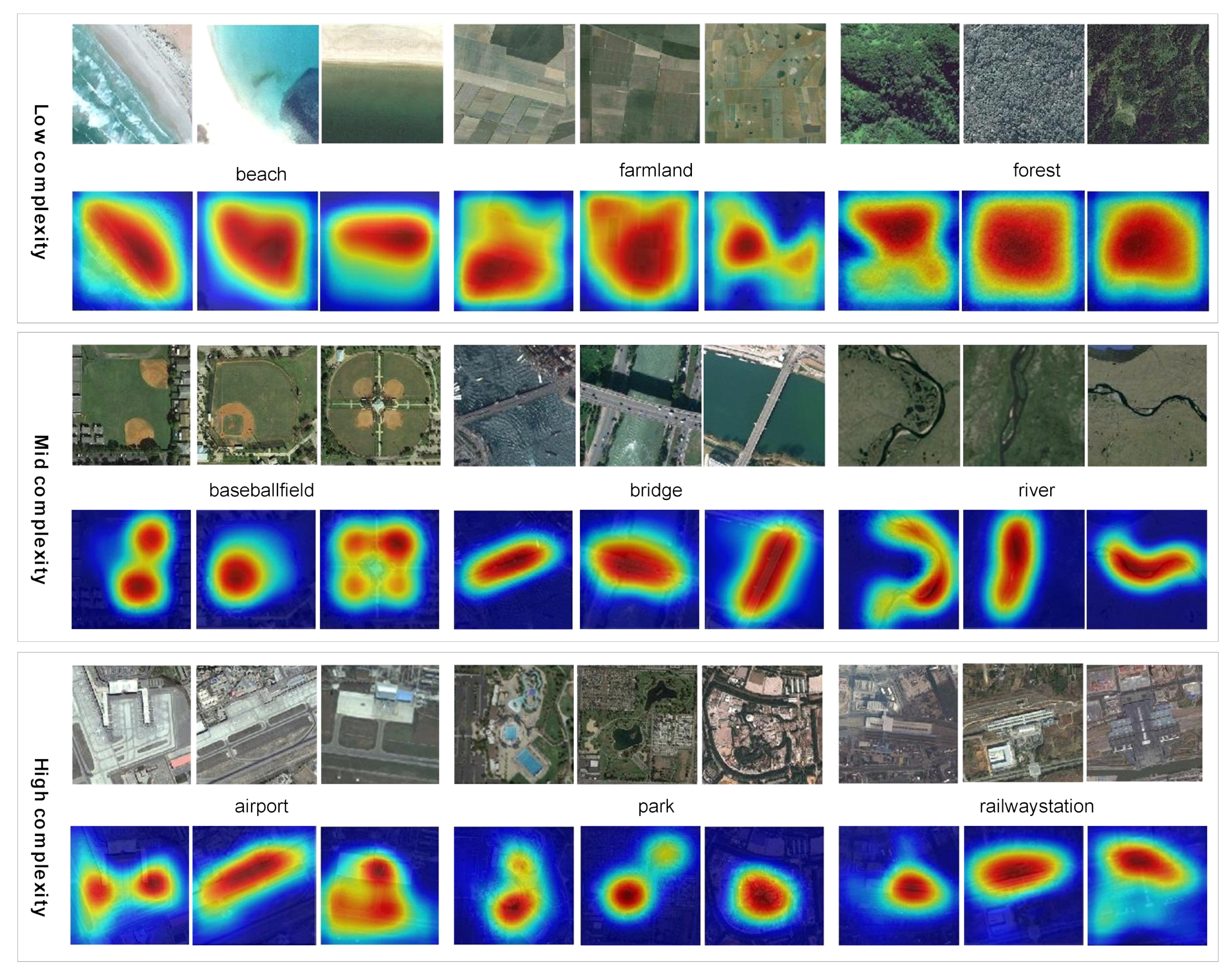
We further explored the distribution pattern combined with scene complexity and found that scenes with high complexity are represented by encoding multiple key objects (Figure 15). The activation mode is monotonous for simple scenes but centered (1–3 objects) on one or more objects for complex scenes.
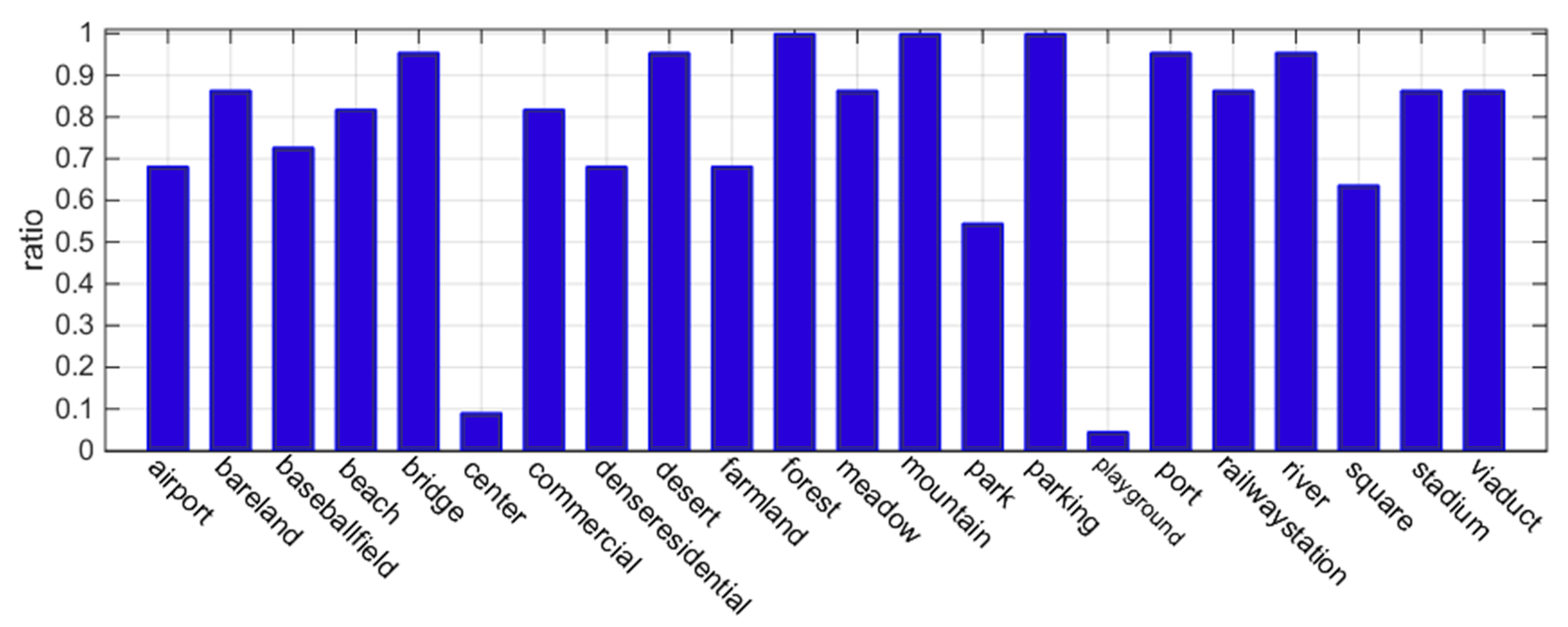
To exclude this phenomenon for only a specific category, we randomly selected 20 samples per class and computed the CAMs. We counted the number of samples that responded to multiple objects (Figure 16). The experimental results demonstrate that the joint representation of various objects supports one scene’s representation. The CAMs of 80% of the samples in the 15 categories, 22, respond to multiple objects. Several complex classes are lower than 50%. These scenes express semantic information through a single entity, such as the center category, representing its concept by individual building.
We conducted similar experiments using the RSI-CB dataset to demonstrate that this phenomenon generalizes to other datasets by occluding multiple objects in a scene and analyzing the corresponding responsive patterns of CAMs (Figure 17). CAMs of the avenue class respond to the trail and the surrounding trees, which indicates that both jointly encode the avenue’s semantic concept. Furthermore, when obscure the trees, the model can only learn the trail features, so the CAMs only respond to the trail area, which causes the model to identify the avenue as a river bridge incorrectly. The results show that the recognition of remote sensing scenes has learned the comprehensive features of multiple targets and that a single target is insufficient to represent the scene.

5. Conclusions

In this paper, we discuss using uniform CNNs to process all images while ignoring the existence of differences in the remote sensing images themselves is unreasonable. We first introduce the scene complexity to metric images’ nature and construct a scene complexity dataset in the remote sensing field. Then, we compare and analyze the effect of hierarchical and scale feature learning on scene recognition with different complexity. We construct a scene complexity prediction framework and use it for depth and scale adaptive models, which effectively improves the recognition accuracy and reduces the model size. Finally, we introduced the interpretable tool CAMs of CNNs to analyze the differences of feature learning patterns for scenes of different complexity, and the experiments show that multiple objects jointly express semantic concepts in complex scenes.
We believe that scene complexity can not only improve the performance of scene recognition, e.g., by improving accuracy and reducing model complexity but can also be extended to other scene understanding tasks. (e.g., segmentation and visual reasoning) and applications. In future work, we will explore how to introduce the information of scene complex to improve these models’ performance. Besides, we will further explore how to improve the semantic representation of complex scenarios using multiple objects’ joint distribution.

Author Contributions

Conceptualization, J.P. and X.M.; methodology, J.P., W.L. and L.H.; validation, X.M. and W.L.; formal analysis, J.P. and L.H.; data curation, B.S.; writing—review and editing, J.P. and H.L.; visualization, J.P. and H.L.; supervision, B.S. All authors read and approved the final manuscript.

Funding

This work was supported by the National Natural Science Foundation of China (grant numbers 61773360, 41871302, and 41871276). This work was carried out in part using computing resources at the High Performance Computing Platform of Central South University.

Institutional Review Board Statement

Not applicable.

Informed Consent Statement

Not applicable.

Data Availability Statement

Parts of related data and models can be found at https://github.com/GeoX-Lab/Scene_Complexity (accessed on 5 February 2021).

Acknowledgments

The Spatiotemporal Data Mining and Information Service Research Group of Central South University helped to process the datasets. The GeoX Group of Central South University provided the hardware.

Conflicts of Interest

The authors declare no conflict of interest.

References

  1. Yang, M.Y.; Liao, W.; Ackermann, H.; Rosenhahn, B. On support relations and semantic scene graphs. ISPRS J. Photogramm. Remote Sens. 2017, 131, 15–25. [Google Scholar] [CrossRef] [Green Version]
  2. Geiger, A.; Lauer, M.; Wojek, C.; Stiller, C.; Urtasun, R. 3d traffic scene understanding from movable platforms. IEEE Trans. Pattern Anal. Mach. Intell. 2013, 36, 1012–1025. [Google Scholar] [CrossRef] [Green Version]
  3. Baek, J.; Chelu, I.V.; Iordache, L.; Paunescu, V.; Ryu, H.; Ghiuta, A.; Petreanu, A.; Soh, Y.; Leica, A.; Jeon, B. Scene understanding networks for autonomous driving based on around view monitoring system. In Proceedings of the 2018 IEEE/CVF Conference on Computer Vision and Pattern Recognition Workshops (CVPRW), Salt Lake City, UT, USA, 18–22 June 2018; pp. 1074–10747. [Google Scholar]
  4. Long, J.; Shelhamer, E.; Darrell, T. Fully convolutional networks for semantic segmentation. In Proceedings of the IEEE Conference on Computer Vision and Pattern Recognition, Boston, MA, USA, 7–12 June 2015; pp. 3431–3440. [Google Scholar]
  5. Ren, S.; He, K.; Girshick, R.; Sun, J. Faster r-cnn: Towards real-time object detection with region proposal networks. IEEE Trans. Pattern Anal. Mach. Intell. 2016, 39, 1137–1149. [Google Scholar] [CrossRef] [PubMed] [Green Version]
  6. Krizhevsky, A.; Sutskever, I.; Hinton, G.E. Imagenet classification with deep convolutional neural networks. In Advances in Neural Information Processing Systems; MIT Press: Las Vegas, NV, USA, 2012; pp. 1097–1105. [Google Scholar]
  7. Shen, L.; Lin, Z.; Huang, Q. Relay backpropagation for effective learning of deep convolutional neural networks. In European Conference on Computer Vision; Springer: Amsterdam, The Netherlands, 2016; pp. 467–482. [Google Scholar]
  8. Alshehhi, R.; Marpu, P.R.; Woon, W.L.; Dalla Mura, M. Simultaneous extraction of roads and buildings in remote sensing imagery with convolutional neural networks. ISPRS J. Photogramm. Remote Sens. 2017, 130, 139–149. [Google Scholar] [CrossRef]
  9. Cheng, G.; Han, J. A survey on object detection in optical remote sensing images. ISPRS J. Photogramm. Remote Sens. 2016, 117, 11–28. [Google Scholar] [CrossRef] [Green Version]
  10. Jain, A.K.; Ratha, N.K.; Lakshmanan, S. Object detection using Gabor filters. Pattern Recognit. 1997, 30, 295–309. [Google Scholar] [CrossRef]
  11. Oliva, A.; Torralba, A. Modeling the shape of the scene: A holistic representation of the spatial envelope. Int. J. Comput. Vis. 2001, 42, 145–175. [Google Scholar] [CrossRef]
  12. Lowe, D.G. Distinctive image features from scale-invariant keypoints. Int. J. Comput. Vis. 2004, 60, 91–110. [Google Scholar] [CrossRef]
  13. Dalal, N.; Triggs, B. Histograms of oriented gradients for human detection. In Proceedings of the 2005 IEEE/CVF Conference on Computer Vision and Pattern Recognition, San Diego, CA, USA, 20–26 June 2005; pp. 886–893. [Google Scholar]
  14. Khan, A.; Sohail, A.; Zahoora, U.; Qureshi, A.S. A survey of the recent architectures of deep convolutional neural networks. Artif. Intell. Rev. 2020, 53, 5455–5516. [Google Scholar] [CrossRef] [Green Version]
  15. Hu, F.; Xia, G.S.; Hu, J.; Zhang, L. Transferring deep convolutional neural networks for the scene classification of high-resolution remote sensing imagery. Remote Sens. 2015, 7, 14680–14707. [Google Scholar] [CrossRef] [Green Version]
  16. Zou, Q.; Ni, L.; Zhang, T.; Wang, Q. Deep learning based feature selection for remote sensing scene classification. IEEE Geosci. Remote Sens. Lett. 2015, 12, 2321–2325. [Google Scholar] [CrossRef]
  17. Chen, C.; Gong, W.; Chen, Y.; Li, W. Object Detection in Remote Sensing Images Based on a Scene-Contextual Feature Pyramid Network. Remote Sens. 2019, 11, 339. [Google Scholar] [CrossRef] [Green Version]
  18. Qu, H.; Zhang, L.; Wu, X.; He, X.; Hu, X.; Wen, X. Multiscale Object Detection in Infrared Streetscape Images Based on Deep Learning and Instance Level Data Augmentation. Appl. Sci. 2019, 9, 565. [Google Scholar] [CrossRef] [Green Version]
  19. Liu, H.; Li, J.; He, L.; Wang, Y. Superpixel-Guided Layer-Wise Embedding CNN for Remote Sensing Image Classification. Remote Sens. 2019, 11, 174. [Google Scholar] [CrossRef] [Green Version]
  20. Xu, Y.; Wu, L.; Xie, Z.; Chen, Z. Building extraction in very high resolution remote sensing imagery using deep learning and guided filters. Remote Sens. 2018, 10, 144. [Google Scholar] [CrossRef] [Green Version]
  21. Egli, S.; Höpke, M. CNN-Based Tree Species Classification Using High Resolution RGB Image Data from Automated UAV Observations. Remote Sens. 2020, 12, 3892. [Google Scholar] [CrossRef]
  22. Taoufiq, S.; Nagy, B.; Benedek, C. HierarchyNet: Hierarchical CNN-Based Urban Building Classification. Remote Sens. 2020, 12, 3794. [Google Scholar] [CrossRef]
  23. Liu, Y.; Suen, C.Y.; Liu, Y.; Ding, L. Scene classification using hierarchical Wasserstein CNN. IEEE Trans. Geosci. Remote Sens. 2018, 57, 2494–2509. [Google Scholar] [CrossRef]
  24. Feixas, M.; Acebo, E.D.; Bekaert, P.; Sbert, M. An Information Theory Framework for the Analysis of Scene Complexity. Comput. Graph. Forum 2010, 18, 95–106. [Google Scholar] [CrossRef]
  25. Moosmann, F.; Larlus, D.; Jurie, F. Learning saliency maps for object categorization. In Proceedings of the Eccv’06 Workshop on the Representation & Use of Prior Knowledge in Vision, Graz, Austria, 7–13 May 2006. [Google Scholar]
  26. Tian, M.; Wan, S.; Yue, L. A Novel Approach for Change Detection in Remote Sensing Image Based on Saliency Map. In Computer Graphics, Imaging and Visualisation; IEEE: Bangkok, Thailand, 2007; pp. 397–402. [Google Scholar]
  27. Isola, P.; Xiao, J.; Parikh, D.; Torralba, A.; Oliva, A. What Makes a Photograph Memorable? IEEE Trans. Pattern Anal. Mach. Intell. 2013, 36, 1469–1482. [Google Scholar] [CrossRef] [PubMed] [Green Version]
  28. Ionescu, R.T.; Alexe, B.; Leordeanu, M.; Popescu, M.; Papadopoulos, D.P.; Ferrari, V. How Hard Can It Be? Estimating the Difficulty of Visual Search in an Image. In Proceedings of the 2016 IEEE/CVF Conference on Computer Vision and Pattern Recognition, Las Vegas, NV, USA, 27–30 June 2016; pp. 2157–2166. [Google Scholar]
  29. Ayromlou, M.; Zillich, M.; Ponweiser, W.; Vincze, M. Measuring scene complexity to adapt feature selection of model-based object tracking. In International Conference on Computer Vision Systems; Springer: Nice, France, 2003; pp. 448–459. [Google Scholar]
  30. Xia, G.S.; Hu, J.; Hu, F.; Shi, B.; Bai, X.; Zhong, Y.; Zhang, L.; Lu, X. AID: A benchmark data set for performance evaluation of aerial scene classification. IEEE Trans. Geosci. Remote Sens. 2017, 55, 3965–3981. [Google Scholar] [CrossRef] [Green Version]
  31. Zeiler, M.D.; Fergus, R. Visualizing and understanding convolutional networks. In European Conference on Computer Vision; Springer: Zurich, Switzerland, 2014; pp. 818–833. [Google Scholar]
  32. Simonyan, K.; Vedaldi, A.; Zisserman, A. Deep inside convolutional networks: Visualising image classification models and saliency maps. arXiv 2013, arXiv:1312.6034. [Google Scholar]
  33. Zhou, B.; Khosla, A.; Lapedriza, A.; Oliva, A.; Torralba, A. Learning deep features for discriminative localization. In Proceedings of the IEEE Conference on Computer Vision and Pattern Recognition, Las Vegas, NV, USA, 27–30 June 2016; pp. 2921–2929. [Google Scholar]
  34. Xiao, J.; Hays, J.; Ehinger, K.A.; Oliva, A.; Torralba, A. Sun database: Large-scale scene recognition from abbey to zoo. In Proceedings of the 2010 IEEE conference on Computer vision and pattern recognition (CVPR), San Francisco, CA, USA, 13–18 June 2010; pp. 3485–3492. [Google Scholar]
  35. Szegedy, C.; Liu, W.; Jia, Y.; Sermanet, P.; Reed, S.; Anguelov, D.; Erhan, D.; Vanhoucke, V.; Rabinovich, A. Going deeper with convolutions. In Proceedings of the IEEE Conference on Computer Vision and Pattern Recognition, Boston, MA, USA, 8–10 June 2015; pp. 1–9. [Google Scholar]
  36. Simonyan, K.; Zisserman, A. Very Deep Convolutional Networks for Large-Scale Image Recognition. arXiv 2015, arXiv:1409.1556. [Google Scholar]
  37. Jia, Y.; Shelhamer, E.; Donahue, J.; Karayev, S.; Long, J.; Girshick, R.; Guadarrama, S.; Darrell, T. Caffe: Convolutional architecture for fast feature embedding. In Proceedings of the 22nd ACM international conference on Multimedia, Orlando, FL, USA, 3–7 November 2014; pp. 675–678. [Google Scholar]
  38. Liu, R.; Lehman, J.; Molino, P.; Such, F.P.; Frank, E.; Sergeev, A.; Yosinski, J. An intriguing failing of convolutional neural networks and the coordconv solution. In Proceedings of the Advances in Neural Information Processing Systems, Montréal, QC, Canada, 3–8 December 2018; pp. 9605–9616. [Google Scholar]
  39. He, K.; Zhang, X.; Ren, S.; Sun, J. Deep residual learning for image recognition. In Proceedings of the IEEE conference on computer vision and pattern recognition, Las Vegas, NV, USA, 27–30 June 2016; pp. 770–778. [Google Scholar]
  40. Zhou, B.; Khosla, A.; Lapedriza, A.; Oliva, A.; Torralba, A. Object Detectors Emerge in Deep Scene CNNs. arXiv 2014, arXiv:1412.6856. [Google Scholar]
  41. McHugh, M.L. Interrater reliability: The kappa statistic. Biochem. Medica 2012, 22, 276–282. [Google Scholar] [CrossRef]
  42. Li, H.; Dou, X.; Tao, C.; Wu, Z.; Chen, J.; Peng, J.; Deng, M.; Zhao, L. RSI-CB: A Large-Scale Remote Sensing Image Classification Benchmark Using Crowdsourced Data. Sensors 2020, 20, 1594. [Google Scholar] [CrossRef] [Green Version]
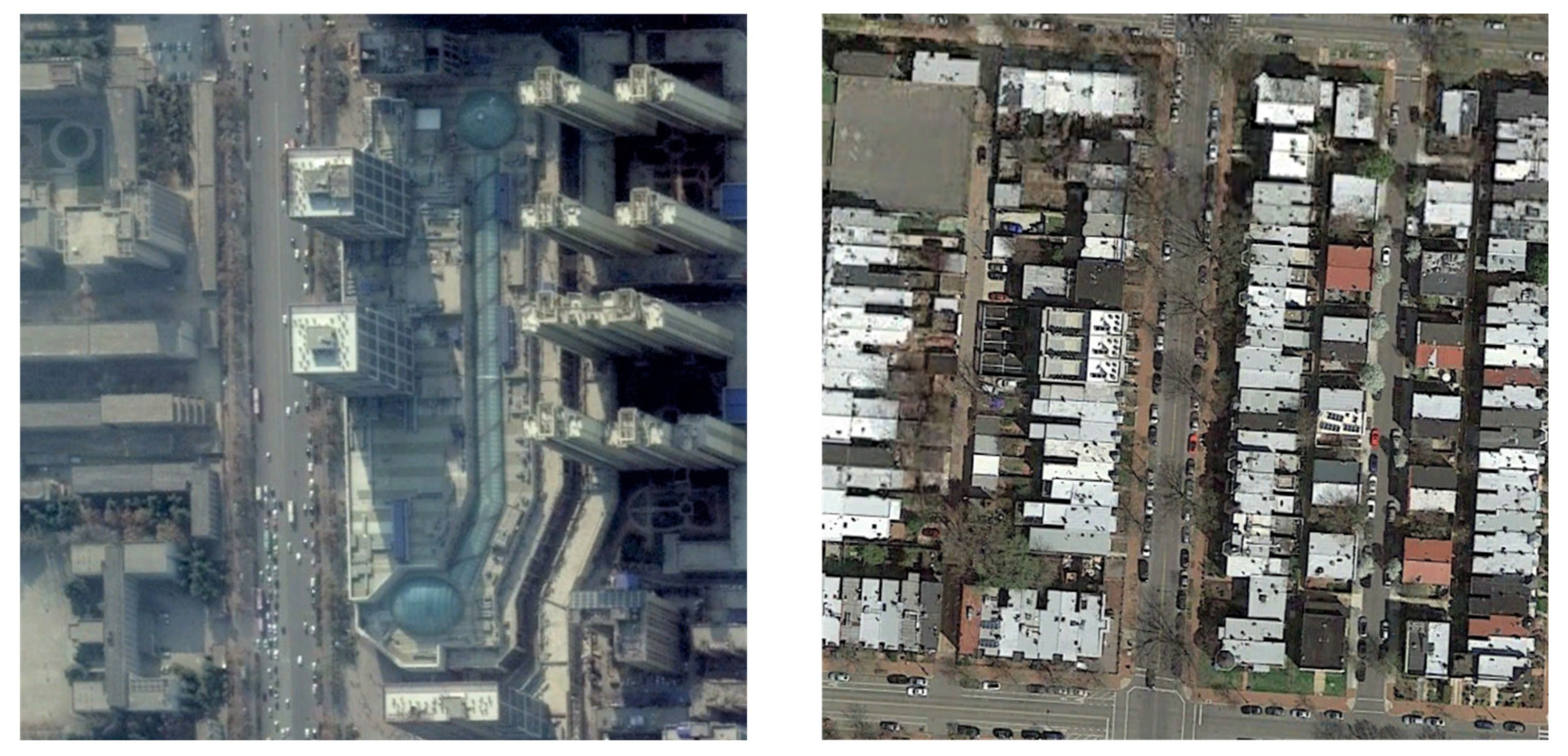
Figure 1. Two similar scenes in content but with different semantic content, left: samples of commercial center; right: samples of dense residential.
Remotesensing 13 00742 g001
Figure 2. Visual memorability evaluation pipeline for sequence testing.
Remotesensing 13 00742 g002
Figure 3. Samples with different scene complexity scores.
Remotesensing 13 00742 g003
Figure 4. Scene complexity score and clustering results for each class of AID-22. It is composed of 3 super-classes according to scene complexity: the low complexity contains 6 classes of scenes, the middle complexity contains 9 classes of scenes, and the high complexity scene contains 7 classes of scenes. Every class contains 360 images, which size is 256 × 256.
Remotesensing 13 00742 g004
Figure 5. The three modified versions of inception V1. The RFs of the last layer before output are 11 × 11 or 47 × 47 or 83 × 83, separately. Nevertheless, the RFs of original inception V1 is the combination ranged from 11 × 11 to 83 × 83.
Remotesensing 13 00742 g005
Figure 6. The pipeline for predicting scene complexity of images. The training process contains three phases: firstly, we train resnet-18 pretrained on ImageNet on the constructed scene complexity dataset. Secondly, we use it to extract features. Thirdly, we utilize the extracted features to train the SVM to predict the scene complexity of images.
Remotesensing 13 00742 g006
Figure 7. The pipeline and CAM calculation. The CAMs represent the contribution of objects on the input images to the prediction, corresponding to the semantic expression. The warmer part means the higher contribution to represent the semantic of an image.
Remotesensing 13 00742 g007
Figure 8. Performance of different inception models for various complex scenes. Top: simple scene, middle: moderate-complexity scene, and bottom: high-complexity scene. The horizontal axis indicates the dimensions 1 × 1, 3 × 3, 5 × 5, and the original multi-scale inception network, and the vertical axis represents the average accuracy of the model tested on a particular complexity class. To compare the variance of accuracy to complexity in the standard range, we limited the y-axis to the same scale (0.25).
Remotesensing 13 00742 g008
Figure 9. Results of the performance of different inception models on various scene complexity categories. Warmer colors indicate higher test accuracy; the x-axis represents the scene complexity category, the y-axis represents the model scale, and the z-axis represents the test accuracy. The multi-scale inception model outperforms the other models in high-complexity scene recognition tasks, but some low-complexity scenes’ accuracy worsens.
Remotesensing 13 00742 g009
Figure 10. Results of the recognition performance of different depth VGG networks on various scene categories. The blue dots indicate the results of the VGG-19 model testing using the dataset, and the red dots indicate the VGG-16 results. The arrow direction shows the change in the accuracy for a particular category.
Remotesensing 13 00742 g010
Figure 11. Recognition results of different complex scenes for various network depths. The horizontal axis represents the models’ various network depths tested on sets from other complexity classes; the vertical axis represents the overall average accuracy.
Remotesensing 13 00742 g011
Figure 12. CAMs of four classes in the AID-22. The warmer the color is, the more outstanding the contribution the region makes to recognition. A lower tone indicates a minimal effect on the prediction result. Similarly, the port category is determined by water and its surrounding areas.
Remotesensing 13 00742 g012
Figure 13. Top-5 CAMs of a sample. From left to right are the top five CAMs in terms of prediction score. GT is the beach category.
Remotesensing 13 00742 g013
Figure 14. CAMs of the marina, city building, crossroad, and dam. These categories are all sampled from RSI-CB dataset.
Remotesensing 13 00742 g014
Figure 15. CAMs of different scene complexity scenes. The top row shows low-complexity scene visualization; the middle row shows moderate-complexity scenes; the bottom row shows the high-complexity scenes. For the farmland object, the activation distribution covers the whole region. However, for the baseball field object, the activated areas are significantly concentrated on a few elements.
Remotesensing 13 00742 g015
Figure 16. The proportion of samples for which corresponding CAMs exhibit a joint multi-object distribution. The horizontal axis represents the scene type, and the vertical axis represents the proportion of samples that respond to multiple objects in the CAMs in each category.
Remotesensing 13 00742 g016
Figure 17. Occluding an object in a scene. Left: GT is an avenue that the model correctly identifies, and CAM responds in the forest and road areas; right: occlude the forest area and the model incorrectly identifies it as a river-bridge, and the corresponding CAM response area mainly concentrates at the road junction.
Remotesensing 13 00742 g017
Table 1. The architecture of revised VGG-16 with adaptive depth.
ConvNet Configuration
VGG-16VGG-16*-AVGG-16*-BVGG-16*-CVGG-16*-D
Conv3-64
Conv3-64
Maxpool
Conv3-128
Conv3-128
Maxpool
Conv3-256
Conv3-256
Conv3-256
MaxpoolMaxpoolMaxpool|GAPMaxpool|GAPMaxpool|GAP
\FC-1024
FC-6
FC-1024
FC-6
FC-1024
FC-6
FC-1024
FC-6
Conv3-512
Conv3-512
Conv3-512
MaxpoolMaxpoolMaxpoolMaxpool|GAPMaxpool|GAP
\FC-1024
FC-9
FC-1024
FC-9
FC-1024
FC-9
FC-1024
FC-9
Conv3-512
Conv3-512
Conv3-512
MaxpoolMaxpoolMaxpoolMaxpoolMaxpool|GAP
FC-4096
FC-4096
FC-22
soft-max
FC-1024
FC-7
soft-max
FC-1024
FC-7
soft-max
FC-1024
FC-7
soft-max
FC-1024
FC-7
soft-max
Table 2. The OA and kappa coefficient results for a multi-scale inception embedded model.
ModelGoogLeNetInception 1 × 1Inception 3 × 3Inception 5 × 5
OA0.83290.68630.77610.7815
Kappa0.82690.67080.76510.7706
Table 3. Overall accuracy tested on the AID-22 scene dataset using the VGG.
ModelTrain Accuracy (%)Test Accuracy (%)
VGG-1696.1594.1
VGG-1996.8994.91
Table 4. The result of depth adaptive VGG-16 on AID-22.
ModelTrain Accuracy (%)Test Accuracy (%)IterationParameters
VGG-1696.1594.10200,000134M
VGG-16*-A97.5694.51240,000343M
VGG-16*-B97.8995.42150,000138M
VGG-16*-C98.1195.80100,00037M
VGG-16*-D97.2094.8680,00012M
Publisher’s Note: MDPI stays neutral with regard to jurisdictional claims in published maps and institutional affiliations.