Abstract
Monitoring the spatial and temporal variability of yield crop traits using remote sensing techniques is the basis for the correct adoption of precision farming. Vegetation index images are mainly associated with yield and yield-related physiological traits, although quick and sound strategies for the classification of the areas with plants with homogeneous agronomic crop traits are still to be explored. A classification technique based on remote sensing spectral information analysis was performed to discriminate between wheat cultivars. The study analyzes the ability of the cluster method applied to the data of three vegetation indices (VIs) collected by high-resolution UAV at three different crop stages (seedling, tillering, and flowering), to detect the yield and yield component dynamics of seven durum wheat cultivars. Ground truth data were grouped according to the identified clusters for VI cluster validation. The yield crop variability recorded in the field at harvest showed values ranging from 2.55 to 7.90 t. The ability of the VI clusters to identify areas with similar agronomic characteristics for the parameters collected and analyzed a posteriori revealed an already important ability to detect areas with different yield potential at seedling (5.88 t ha−1 for the first cluster, 4.22 t ha−1 for the fourth). At tillering, an enormous difficulty in differentiating the less productive areas in particular was recorded (5.66 t ha−1 for cluster 1 and 4.74, 4.31, and 4.66 t ha−1 for clusters 2, 3, and 4, respectively). An excellent ability to group areas with the same yield production at flowering was recorded for the cluster 1 (6.44 t ha−1), followed by cluster 2 (5.6 t ha−1), cluster 3 (4.31 t ha−1), and cluster 4 (3.85 t ha−1). Agronomic crop traits, cultivars, and environmental variability were analyzed. The multiple uses of VIs have improved the sensitivity of k-means clustering for a new image segmentation strategy. The cluster method can be considered an effective and simple tool for the dynamic monitoring and assessment of agronomic traits in open field wheat crops.
1. Introduction
In the last few decades, several studies highlighted the environmental, economic, technical, and practical benefits related to the adoption of precision farming techniques [1,2]. Durum wheat is one of the most important crops worldwide [3], but due to climate change, population increase, and socio-economic factors, it requires specific attention to ensure stable and high yield by optimizing sustainable agronomic management [4]. Grain yield in durum wheat is the result of several morphological and physiological changes during the different growing stages [5]. During cultivation, from an agronomic point of view, different yield components significantly affect grain yield through effects at different growing stages, from sowing to harvest [6,7]. Grain yield in durum wheat can be analyzed in terms of the number of spikes per square meter, number of kernels per spike, and kernel weight, which appear sequentially, with later-developing components under the control of earlier-developing ones [5,8]. Detection of the spatial and temporal variability of the primary components of grain yield during the crop cycle can ameliorate agronomic strategies for improving the environmental, economic, and practical impact of durum wheat cultivation [4,9]. Information regarding crop development is important for monitoring, managing, and predicting grain yield. The high-resolution images can aid in within-season farm management decisions, but also can improve the understanding of the evolution of crop yield [10,11,12]. Recent advances in remote sensing techniques, such as satellite and unmanned aerial vehicle (UAV) images, have meant that a large number of plots can be screened effectively and rapidly [13,14].
The formulation of different vegetation indices derived from multispectral and hyperspectral sensors and cameras is well established, and their application to measure the most important wheat crop parameters is well known [15,16,17]. Spectral vegetation indices derived by remote sensing imagery can be a fast and cost-efficient tool [18,19]. Indeed, the main problem for the utilization of this technique is related to high environmental and crop reflectance variability, which is not well identified by vegetation indices in cases of a lack of agronomic crop sampling (ground truth data). Furthermore, the VIs’ response to plant stresses and agronomic constraints change due to phenological stages (time) and field variability (space) [20]. Since the 2000s, strategies to delineate areas within fields to which management can be tailored have been developed using the clustering algorithm (fuzzy c-means) for assigning field information into potential management zones [21]. In subsequent years, many researches used clustering methods (k-means, partition around mediods, fuzzy c-means), starting from ground data for variable rate application of N fertilizers [22], for estimating wheat biomass, combining a camera sensor and a sensor able to measure crop height [23]. Song et al. [24] studied the delineation of site-specific management zones by Quickbird imagery and the Optimized Soil-Adjusted Vegetation Index (OSAVI). They used a fuzzy k-means clustering algorithm to define management zones and considering the consistent relationship between the crop nutrients, wheat yield, and the wheat spectral parameters. Reza et al. [25] estimated rice yield using RGB images collected by a low-altitude UAV, performing image clustering with graph-cut segmentation (K-means). In a study on winter wheat, the ability of cluster analysis performed on three different vegetation indices (VIs) at anthesis to detect agronomic traits variability of ten cultivars [26] in an open-field experiment was explored. Most of the identified clusters are based on a combination of ground data and satellite or UAV image.
Karnieli et al. [27] highlighted the difficulty in knowing a priori which is the best vegetation index in a given environment. NDVI is widely accepted to characterize canopy growth under different growing conditions. However, NDVI is sensitive to the effects of soil brightness, soil colour, atmosphere, cloud shadow, and leaf canopy shadow, and can fail to distinguish changes in soil cover and plant density from changes in vegetation colour mostly at an early stage of crop development (before tillering), crucial for precision agriculture purposes [28,29,30]. The Soil-Adjusted Vegetation Index (SAVI) was developed as a modification of the NDVI to correct the brightness incidence of the soil, although it was shown to become more sensitive to soil background with the development of crop canopy [31]. The Optimized Soil-Adjusted Vegetation Index (OSAVI) does not depend on the soil line and can eliminate the influence of the soil background effectively [32,33]. OSAVI has been used successfully in wheat for the calculation of aboveground biomass, leaf nitrogen content, and chlorophyll content [4,33,34]. The selection of specific parts of spectral information (e.g., vegetation indices) with a strong correlation with crop proprieties is one way to achieve an affordable and easily implemented instrument in remote sensing for use in the field [35].
The availability of low-cost and high-resolution UAV images allows for the development of more precise and sophisticated methods of image segmentation. Accurate plot segmentation results enabled the extraction of several canopy features associated with biomass yield [36]. Given the importance of monitoring the crop condition, the study reported a novel VI image segmentation method for the precise estimation of agronomic yield traits (yield, biomass, spike number and weight, thousand kernel weight, harvest index) during the most important crop phenological stages. Furthermore, the VI image segmentation was based on the combination of three VI images to improve the VIs’ sensitivity in the detection of dynamic monitoring and classification of wheat yield and yield crop traits.
The present study analysed a classification technique based on spectral information to separate remote sensing data into different groups, using a unsupervised technique such as k-means clustering. The research was performed on seven durum wheat cultivars. Data of three VIs (NDVI, SAVI and OSAVI) collected by a high-resolution UAV were clustered (Ward’s minimum variance approach) at different crop stages (seedling, tillering, and flowering) for delineating clusters area with homogeneous VI values. UAV imagery data were clustered, combining data for three VIs for evaluating a new study approach on remote sensing images in precision agriculture with the aim of improving k-means cluster and completely limit the needs of field data. Agronomic traits (yield and yield components) collected during the crop cycle were used to validate the VI cluster findings and analyze the agronomic crop growth dynamic and classification at every single stage. Furthermore, identified VI clusters at seedling, tillering, and flowering were related to the agronomic yield data collected at harvest. Crop trait dynamics and variability were analyzed. The study aimed to analyze the ability of the cluster method applied to high-resolution UAV VI data to detect yield and yield component dynamics during the crop cycle.
2. Materials and Methods
2.1. Study Area
On-farm research was carried out in the 2016 crop season in the Marche Region (Central Italy—411135.31E, 4730500.51N; UTM-WGS84 zone 33N Italy). Seven durum wheat cultivars (Odisseo, Monastir, Ramirez, Ariosto, Clovis, Pigreco, and Zetae) were cultivated in an area of about 6 ha, with each cultivar covering 800 m2 with plot dimensions of 25 m × 32 m (Figure 1). Minimum tillage was used to prepare a suitable seedbed, and seeding was performed with 220 kg of seeds per hectare in October 2015. The cultivars were harvested in July 2016. Phosphorous was incorporated at sowing (220 kg ha−1—P2O5 (27%)), Nitrogen was spread at sowing, tillering, and stem elongation with 40, 160, and 160 kg ha−1, respectively, of N (36%) SO3 (23%)). The pest control scouting and weed control were carried out with chemical pesticides during the crop cycle.
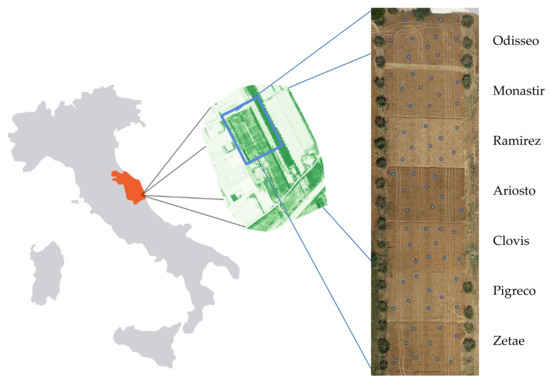
Figure 1.
Left image: Study area (NDVI image). Middle image: Durum wheat cultivars (RGB image at harvest). Right image: Sixty-five georeferenced ground truth areas collected at harvest.
The meteorological conditions were typical of Mediterranean countries, with low temperature and high precipitation in the period October –March (minimum temperature −2 °C, precipitation 450 mm), while higher temperatures and low precipitation were recorded in April–July (maximum temperature 34 °C, precipitation 210 mm).
2.2. Field Measurements
The phenological stages of the wheat crops were periodically recorded according to the Zadoks cereal-growth-staging scale (ZS) [37]. At each crop stage, 65 georeferenced areas of 0.5 m2 were hand cut. Whole plant dry mass (g m−2) was determined after oven drying the fresh plant material at 65 °C for 48 h. Furthermore, crop yield (t ha−1), spike number, spike weight (g m−2), thousand kernel weight, and harvest index (H index = yield/biomass) were analyzed at harvest (99 ZS, July 14). Crop yield was expressed as t ha−1 according to crop harvest data (1 t ha−1 = 100 g m−2). Ground truth data were georeferenced with GPS Leica model Viva GS15 (Leica Geosystems AG, Heerbrugg, Switzerland) horizontal and vertical accuracy of 25 and 35 mm, respectively.
2.3. UAV System
The crop was monitored with the high-resolution eBee UAV system (senseFly, Cheseaux-sur-Lausanne, Switzerland) (Figure 2). Flight missions were performed at three stages: seedling growth (13 ZS, 26 February), at tillering (25 ZS, 3 April), and at flowering (65 ZS, 18 May). Remote sensing data were collected using two cameras, Canon Powershot S110 and Canon Powershot S110 NIR camera (0.7 kg weight, 12 million pixels resolution, 5.58 × 7.44 mm2 sensor size, 1.33 μm pixel pitch, RAW JPEG format images). The S110 was used for collecting RGB images and visible spectrum images, while the S110 NIR Camera was used for collecting data related to near infra-red (850 nm), red (625 nm), and green (520 nm).
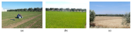
Figure 2.
Pictures of the experimental field at seedling (a), tillering, (b) and harvest (c).
2.4. Flight Missions
The UAV campaign was conducted between 12:00 and 14:00 local time. Flights were carried out on a total surface of about 8 hectares, at a flight altitude of 100 m above ground level (AGL) in stable ambient light conditions, with high visibility and wind below 5 m s−1. Forty-four overlapping pictures from each camera were used to obtain an 80% frontal overlap and an 80% side to avoid geometric distortion for mosaicking to produce an ortho-image. The autopilot analyzes (continuously) the inertial measurement unit (IMU) and onboard GPS data to control every aspect of the eBee’s flight. The integration of the UAV and sensors with GPS and IMU enables obtaining direct georeferencing imaging after image processing. Across the field, ten calibrated reflectance panels (CRP) were used to apply radiometric calibration to the acquired images (fixed targets). The CRP were distributed at the beginning of the season to obtain at each flight the photogrammetric imagery with uniform horizontal and vertical accuracy, and to overlay the measurements from multiple dates.
2.5. Data Processing
Ortho-mosaicking of acquired images was elaborated with the Pix4D software package, which incorporates a scale-invariant feature transform (SIFT) algorithm to match key points across multiple images [38]. The multiple overlapped images were stitched together and ortho-rectified. The data processing started with initial processing (camera internals and externals, automated aerial triangulation, bundle block adjustment); the second step was the point cloud densification, and finally the ortho-mosaic generation. Ortho-rectification by aero-triangulation and mosaicking were elaborated. A certificate of the calibration of Canon cameras was uploaded in the software to optimize internal camera parameters (focal length, principal points, lens distortions). The ortho-rectification starts from the exterior position and orientation parameters provided by the UAV system (pitch, roll, yaw angles) and CRP. The geometric resolution on the ground (GSD) of the acquired images was 2 cm pixel−1. The final output was one RGB and one false-color orthophoto with an NIR band in the GeoTIFF format with a resolution of 5 cm2 pixels (georeferenced to UTM-WGS84 zone 33N Italy). Starting from the GeoTIFF images, vegetation indices were calculated by the index calculator function of Pix4D. The Normalized Difference Vegetation Index (NDVI), the Soil-Adjusted Vegetation Index (SAVI), and the Optimized Soil-Adjusted Vegetation Index (OSAVI) layers were generated in a raster calculator from extracted red (R) and near infra-red (NIR) channels. The ten CRP with a known albedo were used to calibrate the NIR camera. GeoTIFF images and georeferenced sampling data were processed for agronomic purposes with QGIS [39].
2.6. Vegetation Indices
The Normalized Difference Vegetation Index (NDVI), the Soil Adjusted Vegetation Index (SAVI), and the Optimized Soil Adjusted Vegetation Index (OSAVI) were calculated according to the formula reported in Table 1.

Table 1.
Vegetation indices abbreviation, name, formula, and references.
The NDVI values for vegetation range from 0 to 1, and positive values are related to increasing greenness. NDVI has some weaknesses linked to the possibility of reaching saturation, in particular in later growth stages [43,44]. The OSAVI index was proposed by using bidirectional reflectance in the near-infrared and red bands. OSAVI does not depend on the soil line and can eliminate the influence of the soil background effectively [28]. The soil adjustment coefficient (0.16) was selected as the optimal value to minimize the variation with the soil background. The soil-adjustment factor L in the SAVI equation varies from 0 to 1 according to the canopy density. L decreases with increases in vegetation amount. According to the above-cited papers, L value was set at 0.5 for the seedling stage, at 0.30 for the tillering stage, and 0.20 for the anthesis stage [19,45,46].
2.7. Statistical Analysis
The NDVI, OSAVI, and SAVI data recorded at each crop stage (seedling, tillering, flowering) were statistically processed using cluster analysis (Ward’s minimum variance approach) [47]. The procedure was described in Marino et al. [39]. The statistical VI median values, standard deviations, and analysis of variance between and within the clusters are reported in Table 3 (seedling stage), in Table 4 (tillering stage), and Table 5 (flowering stage). Statistical tests were used to verify the dependence conditioning of the different variables (a posteriori). The scree plot to identify the significant number of clusters was used (Appendix A, Figure A1) [48]. Non-parametric ANOVA by the Kruskal–Wallis test [49] was used when the measurement variable does not meet the normality assumption, while ANOVA was used when the variable met the normality assumption. OriginPRO 8 (Origin Lab Corporation, Northampton, MA 01060, USA) and STATISTICA (Stat Soft., Inc., Oklahoma, OK, USA) were used for statistical analysis.
3. Results
In the present paper, three flight missions were carried out at the seedling, tillering, and flowering stages. Cluster analysis (Ward’s minimum variance approach) of the three VIs’ data were elaborated. Cluster areas with homogeneous VI values were identified at each crop stage. Yield and yield components collected during the crop cycle were used to validate the VI cluster findings. The identified VI clusters at seedling, tillering, and flowering were related to the agronomic yield data collected at harvest to evaluate the crop trait dynamics and the ability to identify different crop areas during the crop cycle. The yield data of the whole field at harvest were for cv. Ariosto, 6.7 t ha−1, for cv. Ramirez, 6.2 t ha−1, Monastir, 5.9 t ha−1, Odisseo and Clovis, 5.6 t ha−1, Pigreco, 5.1 t ha−1 and Zetae, 5 t ha−1.
Figure 3 reports the images of the three VIs at three different growth stages. At seedling, the NDVI value ranged from a minimum value of 0.12 for the cultivars Zetae and Ramirez to a maximum value of 0.69 for the cultivars Odisseo, Ariosto, and Pigreco. The SAVI and OSAVI showed the same trend, with lower values of 0.2 and 0.14 and maximum values of 0.88 and 0.76 for SAVI and OSAVI, respectively. At the tillering stage, the minimum value for NDVI was recorded by cv. Pigreco (0.13) and maximum by cv. Ariosto (0.91), while SAVI and OSAVI showed a minimum value for the same cultivars with values of 0.2 and 0.18, respectively, and the highest values of 1.0 and 0.96. The cultivars with the lower and higher values were the same. At the flowering stage, the NDVI value ranged from 0.17 to 0.94, SAVI from 0.22 to 1.06, and OSAVI from 0.19 to 1.02. The lowest value was recorded for the cultivar Zetae, and the highest for the cultivar Ariosto.
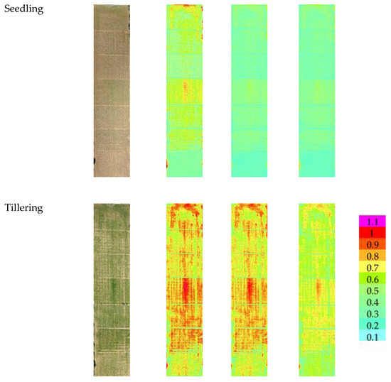
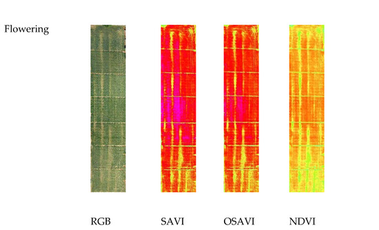
Figure 3.
RGB, Soil-Adjusted Vegetation Index (SAVI), Optimized Soil-Adjusted Vegetation Index (OSAVI), and Normalized Difference Vegetation Index (NDVI) maps at different crop stages: seedling, tillering, and flowering growth stage. Maps were elaborated by Pix4D and QGis software.
Table 2 shows the statistical parameters of the seven durum varieties and data distribution to analyze the pixel frequency trend, useful for detecting differences between cultivars. NDVI data of pixel frequency distribution related to the cultivars were reported, SAVI and OSAVI pixel frequency distribution show a similar trend (data not shown). The pixel frequency distribution of NDVI for each cultivar at seedling stage showed that the highest median data recorded for the cv. Ariosto, followed by cv. Clovis and cv. Odisseo (Table 2). The cultivars Ramirez, Pigreco, and Monastir showed a lower median value (by about −12%) compared to Ariosto. Zetae showed the lowest median value (−36%) compared to Ariosto. At tillering, the median value of cv. Ariosto and Clovis, followed by cv. Pigreco as a close second, showed the greatest distribution of NDVI values towards higher values. The cv. Odisseo, Monastir, and Ramirez showed median values and population distribution towards lower NDVI values (by about −6%), and the cv. Zetae showed lower NDVI values than all other cultivars, with median pixel frequency distribution values 15% lower than cv. Ariosto and Clovis. At flowering, the cultivars Ariosto, Monastir, Ramirez, and Clovis showed a high median value while, on the contrary, the cultivars Zetae, Pigreco, and Odisseo showed the lowest median value.
Table 2.
NDVI pixel frequency distribution of the durum wheat cultivars at seedling, tillering, and flowering (mean, median, standard deviation, variance, minimum, maximum, median absolute deviation (MAD) and pixel count).
3.1. Seedling: VI Cluster Map
The cluster map, elaborated starting from NDVI, OSAVI and SAVI indices taken at seedling, is reported in Figure 4. Four clusters were identified, the highest values are represented by cluster 1. The median value, standard deviation, and analysis of variance of each VI cluster’s data are reported in Table 3. NDVI and OSAVI ranged from 0.43 for cluster 1 to 0.24 for cluster 4. The SAVI values appeared more spaced apart (0.66 for cluster 1; 0.37 for cluster 4). The differences recorded among the mean value of each cluster showed the same trend for all the VIs.
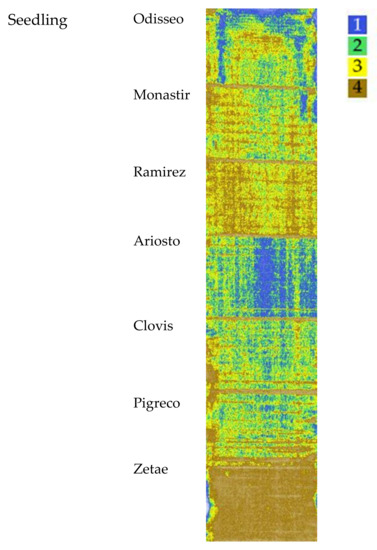
Figure 4.
Map of the Vis’ spatial variability of the seven cultivars clustered by Ward’s method at seedling. Cluster 1 indicates the highest VI values, while cluster 4 indicates the lowest.
Table 3.
Vegetation indices’ (VIs) median values, standard deviations, and analysis of variance of clusters identified by Ward’s cluster method at seedling stage. The median values are assumed as a measure of central tendency in case of not symmetrical data distribution.
VI Cluster Map at Seedling and Agronomic Traits Dynamic Analysis
Agronomic traits data collected at seedling stages were used to analyze and evaluate the ability of the VI cluster map to provide crop yield information at the time of sampling and the evolution during the season up to harvest. As expected, differences in biomass at seedling were low, ranging from 130.8 g m−2 for Ramirez and to 90.9 g m−2 for Clovis: statistical analysis showed no significant differences among cultivars (data not shown).
The agronomic data collected at harvest on the 65 georeferenced points used for cluster analysis were grouped in a box plot (Figure 5) according to the identified clusters of the seedling clusters map. All yield components showed significant differences among clusters, except thousand-kernel weight and harvest index (H index). The yield median value of the cluster 1 was 5.82 t ha−1, while cluster 2 showed a median value of 5.62 t ha−1, cluster 3 had a median value of 4.62 t ha−1 and cluster 4 had a mean value of 4.22 t ha−1. The trend was confirmed by yield component data, with the highest value for aboveground dry biomass, spike weight, and spikes per square meter recorded by cluster 1 followed by cluster 2 (−5 to 15%), by cluster 3 (−20 to 27%), and by cluster 4, with a crop trait value reduction of 32–35%. H index and spike weight showed an opposite trend, as expected. In the first cluster, cv. Ariosto was the most represented (50% of samples), which confirmed the higher index value even if some samples showed low average values (even 4 t ha−1). In the second cluster, there was a greater presence of all cultivars. Cluster 2 showed yield values that were much higher than the related spectroradiometric values for some areas of cv. Monastir and Clovis (about 7.7 t ha−1). In the third cluster, there was a greater representation of all cultivars with higher yield value for some areas of Ramirez (7.5 t ha−1) and lower yield value (lower than 4 t ha−1) for some samples of cv. Odisseo, Monastir, Ramirez, Clovis, and Pigreco. In cluster 4, 50% of all samples belonged to the Zetae cultivar, with yield values not always being among the lowest (average value of 5 t ha−1) and one value being close to 7 t ha−1.
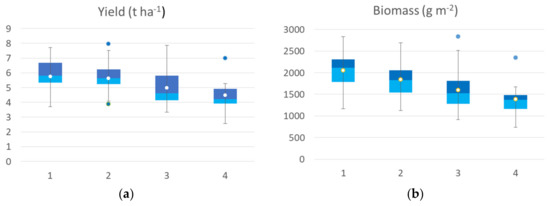
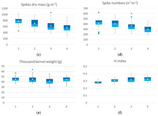
Figure 5.
Box plot of agronomic traits collected at harvest: yield (a), biomass (b), spike weight (c), spike number (d), thousand-kernel weight (e) and harvest index (f) of the seven durum wheat cultivars grouped according to the 4 identified VI clusters at seedling. All the components showed a significant difference among clusters, and thousand kernel weight showed no significant differences among clusters (Kruskal–Wallis test).
3.2. Tillering: VI Cluster Map
The map, elaborated starting from NDVI, OSAVI, and SAVI indices at the tillering stage, with the four identified clusters, is reported in Figure 6. The median values of VI clusters identified at tillering are reported in Table 4; values ranged from 0.72 for cluster 1 to 0.40 for cluster 4 (NDVI). The SAVI and OSAVI values are even more differentiated (0.87–0.84 for cluster 1; 0.48–0.46 for cluster 4, respectively). The trend was the same for all VIs.
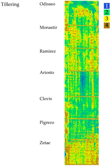
Figure 6.
Map of the VIs’ spatial variability of the seven cultivars clustered by Ward’s method at tillering. Cluster 1 indicates the highest VI values, while cluster 4 indicates the lowest.
Table 4.
Vegetation indices’ (VIs) median values, standard deviations, and analysis of variance of clusters identified by Ward’s cluster method at tillering stage. The median values are assumed as a measure of central tendency in the case of asymmetrical data distribution.
VI Cluster Map at Tillering and Agronomic Traits Dynamic Analysis
At the tillering stage, the aboveground dry biomass showed the highest value for the cultivars Ariosto, Clovis, and Pigreco (about 370 g m−2) followed by Zetae (−5%) and by Odisseo, Monastir, and Ramirez (−10%). The number of spikes per square meter showed the highest value for Ariosto (mean values of 428) and the lowest for Clovis (354). The dry weight and spikes per square meter data showed similar ranges (data not shown).
The cultivars Ariosto, Clovis, and Pigreco showed an important area in cluster 1 The cultivars Ramirez, Monastir, Odisseo, and Zetae showed high numbers of ground data classified in the lower cluster and an important surface classified as clusters 3 and 4 and a high frequency of pixels with values included in clusters 3 and 4.
The agronomic data collected at harvest, classified according to the identified clusters at tillering, are reported in Figure 7. All of the yield components showed significant differences among clusters, except for the thousand kernel weight. Yield data of ground points that fall back into the cluster 1 at tillering showed higher values of all agronomic parameters collected at harvest compared to the other three clusters. The median value of the yield calculated by grouping the samples falling into cluster 1 was 5.66 t ha−1, cluster 2 showed a median value of 4.74 t ha−1, cluster 3 showed a median value of 4.31 t ha−1, cluster 4 had a mean value of 4.66 t ha−1. The trend was confirmed by yield components data, with the highest value for biomass, spike weight, and spikes per square meter recorded by cluster 1 followed by cluster 2 (−25 %), cluster 3 (from −26 to −29%), and cluster 4, with a crop trait value reduction by 28-33%. H index and spike weight showed an opposite trend, as expected.
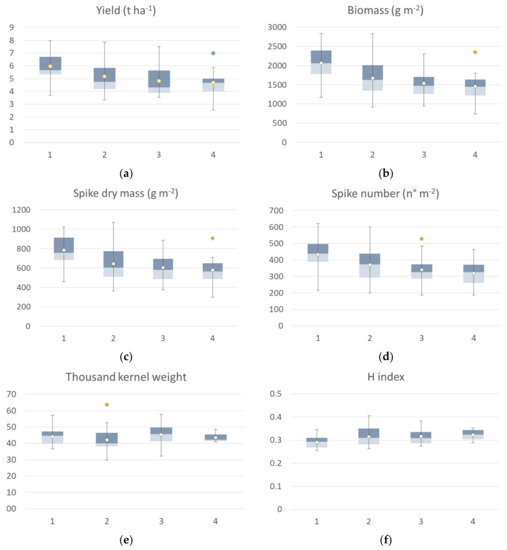
Figure 7.
Box plot of agronomic traits collected at harvest: yield (a), biomass (b), spike weight (c), spike numbers (d), thousand-kernel weight (e) and H index (f) of the seven durum wheat cultivars grouped according to the four identified VI clusters at tillering. All the components showed a significant difference among clusters, and thousand kernel weight showed no significant differences among clusters (Kruskal–Wallis test).
3.3. Flowering: VI Cluster Map
The map, elaborated starting from NDVI, OSAVI and SAVI indices at the flowering stage, with four identified clusters, is reported in Figure 8, while the median values of the VI clusters identified at flowering are reported in Table 5. Identified clusters showed a median value for NDVI of 0.86 for cluster 1, 0.81 for cluster 2, 0.74 for cluster 3, and 0.59 for cluster 4. The SAVI and OSAVI values are even more differentiated (1.06–1.02 for cluster 1; 0.71–0.68 for cluster 4, respectively). The differences recorded between the mean values of each cluster showed the same trend for all the VIs.
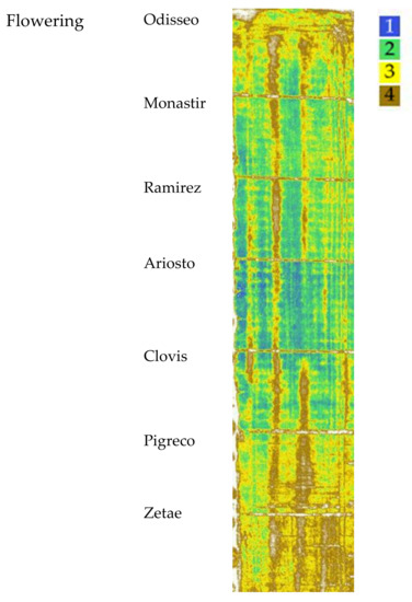
Figure 8.
Map of the VIs’ spatial variability of the seven cultivars clustered by Ward’s method at flowering. Cluster 1 indicates the highest VI values, cluster 4 indicates the lowest.
Table 5.
Vegetation indices’ (VIs) median values, standard deviations and analysis of variance of clusters identified by Ward’s cluster method at flowering stage. The median values are assumed as a measure of central tendency in the case of asymmetrical data distribution.
VI Cluster Map at Flowering and Agronomic Trait Dynamics Analysis
At flowering stage, the aboveground dry biomass had the highest value for the cultivars Ariosto, Clovis, and Pigreco (970 g m−2), followed by Zetae (−5%), and then by Odiseo, Monastir, and Ramirez (−12%). The number of spikes per square meter showed the highest value for Ariosto (mean of 450) and the lowest for Clovis (mean of 372). The cultivar Zetae showed a different spectroradiometric response and VI values. The cultivars Ariosto, Clovis, Pigreco, and Monastir showed a high number of data in cluster 1 identified by the VI cluster map and confirmed by the high values of VI pixel frequency distribution. On the other hand, the cultivars Zetae, Ramirez, and Odisseo showed a high number of ground data classified in the lower cluster.
The agronomic data collected at harvest, classified according to the identified clusters, are reported in Figure 9. Yield data of ground points that fall into cluster 1 identified at flowering showed a high value of all agronomic parameters collected at harvest compared to the other clusters. The median value of the yield calculated by grouping the samples falling in cluster 1 was 6.44 t ha−1, while cluster 2 showed a median value of 5.6 t ha−1, cluster 3 had a median value of 4.31 t ha−1, and cluster 4 had a mean value of 3.85 t ha−1. The trend was confirmed by yield component data, with the highest values for the aboveground dry biomass, spike weight, and spike for square meters recorded by cluster 1, followed by cluster 2 (−14 to −25 %), cluster 3 (−27 to −34%) and cluster 4, with a crop trait value reduction of −40 to −50%. H index and spike weight showed an opposite trend, as expected, and thousand kernel weight showed no significant differences among clusters.
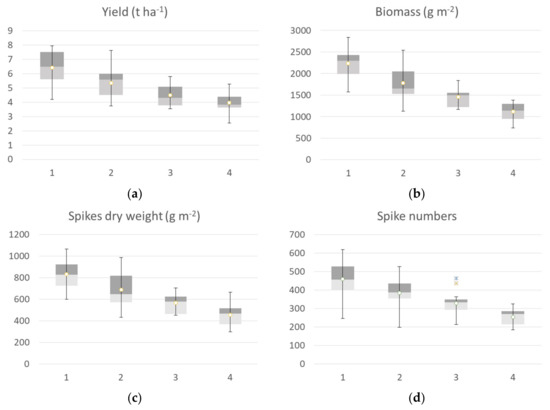
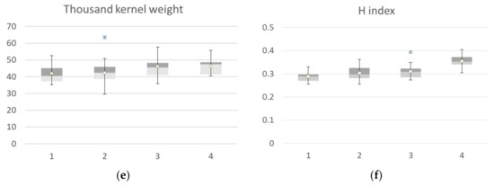
Figure 9.
Box plot of Agronomic traits collected at harvest: yield (a), biomass (b), spike weight (c), spike numbers (d), thousand-kernels weight (e) and harvest index (f) of the seven durum wheat cultivars grouped according to the 4 identified VI clusters at flowering. All the components showed a significative difference among clusters, while thousand kernel weight showed no significant differences among cluster (Kruskal–Wallis test).
4. Discussion
Wheat yield is the result of crop genetic characteristics, environmental conditions, and agronomic management strategies. Yield components are a snapshot of the final composition of yield [50]; however, a dynamic view of the generation of yield components is crucial for the application of precision agriculture. As reported by Schirrmann et al. [51], during the crop cycle, at a single stage, a UAV flight mission can provide high-resolution vegetation indices data useful for agronomic field management. The agronomic crop field management strategies can be related both to crop and environmental needs, aiming at improving crop yield and sustainability and reducing the intensive use of energy.
Simple VIs combining visible and NIR bands have significantly improved the sensitivity of the detection of green vegetation. Each VI has its specific expression of green vegetation, its suitability for specific uses, and some limiting factors [28,52]. Moreover, simple, fast and effective systems that can use the information produced by the VIs with an agronomic sense still need to be developed.
Xue and Su [28] pointed out, for practical applications, that the choice of a specific VI needs to be made with caution by comprehensively considering and analyzing the advantages and limitations of existing VIs and then combine them to be applied in a specific environment.
Accurate plot segmentation results allow the extraction of several canopy features associated with biomass yield [36]. The contribution of this study to precision agriculture is to show that an image segmentation technique (Ward’s method) combined with multiple VI images collected by high-resolution UAV at different growing stages can improve Vis’ sensitivity, allowing more accurate wheat dynamic monitoring.
The three indices derived from the same wavelengths with different sensitivity (NDVI, SAVI and OSAVI) were clustered to analyze the ability of cluster methods to group VI data of seven wheat cultivars according to the agronomic yield and yield components spatial and temporal variability. The validation process was made through direct correlations between obtained VIs and the vegetation characteristics of interest measured at the same time of flight and harvest.
VI data of SAVI, OSAVI and NDVI showed the same trend: SAVI showed values higher than OSAVI and NDVI, respectively. The range of SAVI and OSAVI was higher than NDVI, especially at seedling stage (NDVI −34% related to SAVI) but also to tillering and flowering (NDVI −18 and −23%, respectively, related to SAVI). The results of the experiment agree with studies on winter wheat [26]. The pixel frequency distribution of VIs showed a difference among cultivars, with high values for cv. Ariosto, Clovis, and Monastir and lower values for Pigreco and Zetae.
Data of NDVI, OSAVI and SAVI were clustered according to Ward’s minimum variance method for identifying significant homogeneous VI area. The scree plot analysis was used to contrast the distances against the number of clusters for detecting the distinctive break (elbow), which indicates the number of clusters to retain [53]. The number of identified clusters at seedling, tillering and flowering was four. At each growing stage, clustered images and harvested yield data, grouped according to VIs identified cluster, were analyzed a posteriori. Furthermore, cultivars’ agronomic traits dynamically collected at a single crop stage were compared to VI clustered images to validate the results. The high values of the indices were in most cases, but not always, correlated to high values of the agronomic parameters, confirming VIs as a valuable tool for wheat genotype yield assessment, as well as the importance of the spectral response of every single variety for the understanding of remote sensing data [54]. In the open field experiments, the cv. Ariosto, Ramirez, and Monastir were the most productive at harvest, followed by cv. Odisseo and Clovis (about 15%) and Pigreco and Zetae (about −23%).
4.1. Seedling: VI Cluster Map and Agronomic Traits Dynamic Analysis
The VI cluster map at seedling showed significant differences among clusters. Related to the first cluster, the mean differences were −14% for cluster 2, −37% for the third cluster, and −44% for the fourth cluster. The agronomic biomass data collected at seedling showed no significant differences among cultivars related to the low biomass values. Many references and papers highlighted the problem related to the early stage identification and detection of spatial variation on biomass and the difficulty of identifying regression among VIs and agronomic data [55]. Despite data meaning, the cultivars Zetae showed a high number of biomass values classified in the lower cluster, confirming the VI cluster images (Figure 4). The different spectroradiometric response (especially for the cultivar Zetae and in some cases the c.v. Ariosto) confirms the results of Kipp et al. [56], who tested the suitability of spectral reflectance for the evaluation of the early plant vigor of winter wheat cultivars. The authors observed a significant correlation between pixel analysis and vegetation index (EPVI Adj. R2 = 0.55), and at the same time, they could observe that the plant vigor is a cultivar-specific trait.
The agronomic data collected at harvest and grouped in a box plot according to the identified clusters showed a clear identification of the most productive areas at harvest.
Cluster 2 showed close values to cluster 1; cluster 3 and 4 were closer (−21% and −27% related to cluster 1, respectively). The trend was confirmed by yield component data.
The cultivar with the highest production at harvest showed the highest number of samples in cluster 1. Cluster 2 showed yield values that were much higher than the related spectroradiometric values due to some areas of cv. Monastir and Clovis. In the third cluster, there was a greater representation of all cultivars. Cultivar Zetae, with yield values not always among the lowest, showed a big area in cluster 4.
From an agronomic point of view, the yield-determining physiological processes such as adaptation to environments with a broad range of climatic and edaphic variation, diversity in plant traits, and plasticity in source–sink relationships are well known [57]. Yield data confirm that, at the seedling stage, the identified cluster significantly distinguishes the more productive areas from the less productive ones. Despite the fact that the low biomass collected at seedling makes it difficult to find significant correlations, VI clusters identified areas with potentially fewer limiting factors. The study reported by Rasmussen et al. [58] showed that VIs based on UAV imagery have the same ability to quantify crop responses to experimental treatments as ground-based recordings with cameras and advanced sensors, excluding problems related to sensor accuracy. Moreover, as reported by different researchers, OSAVI and SAVI excel in regions with sparse vegetation where the soil is visible through the plants [59]. Consequently, the present study confirms that the utilization of a VI that corrects for soil interference, such as SAVI and OSAVI, worked the best when wheat leaf area was at its lowest and bare soil was at its greatest out of all of the sampling times [19,26].
The combination of the three indices to define clusters starting from remote sensing data proved that measurements at an early growing date, while the plants are still seedlings, are optimal for the assessment of the future yield.
4.2. Tillering: VI Cluster Map and Agronomic Traits Dynamic Analysis
The map elaborated at tillering stage showed a significant difference among the clusters. Related to the first cluster, the median differences were −12.5% for cluster 2, −27% for the third cluster, and −44.5% for the fourth cluster.
The cultivars Ariosto, Clovis, and Pigreco showed the highest values of agronomic parameters collected at tillering, the highest numbers of agronomic ground data in cluster 1, and the highest frequency of high VI values. Besides the cultivar Zetae, the cultivars Ramirez, Monastir and Odisseo also showed high numbers of ground data classified in the lower cluster, confirming the VIs’ ability to detect real-time plant status.
Comparing harvest data to the identified cluster, although statistical analysis has been able to distinguish different cultivars, an important overlap was found between clusters 3 and 4 for many agronomic parameters. VI data at tillering were not able to identify areas that were more productive at harvest than expected. Many papers reported the weak relationship between VIs and yield at tillering. Chandel et al. [60] in an experiment at four different phenological stages (tillering, booting, heading, and milking) found a lower value of correlation coefficient and coefficient of determination at tillering (NDVI = 0.6). Fu et al. [34], in an experiment with UAV and multi-spectral cameras on a wheat canopy at key growth stages, found that the yield estimation (predicted yield) based on UAV images at the tillering stage was poor.
The yield variability differences recorded at harvest by cluster 1 and the other clusters were related to the number of spikes per m2. The results are in accordance with Slafer et al. [50], who reported the number of spikes as the main responsible factor for coarse regulations driven by environmental factors. Although the VIs detected a radiometric difference among cluster 2, 3 and 4, the lower yield differences recorded at harvest can be explained by the ability of any yield component to act as a fine-tuning mechanism, so the plasticity of the yield components can accommodate changes in yield and by the sudden change in the structure of the plant, which can have different times in different cultivars [61]. Furthermore, it is well known that the different tillering capability (at the tillering stage) in the various genotypes has been recognized as the main plasticity trait in response to different environmental conditions (soil characteristics, water and nitrogen availability) [62]. An important difference found in this experiment is that at tillering, the largest range of VI values was recorded. Areas with VI values comparable to the values of seedling and other areas comparable to the values recorded at flowering were detected. This variability in the spectroradiometric response, combined with the statements above, can justify the difficulties in detecting crop trait dynamics.
4.3. Flowering: VI Cluster Map and Agronomic Traits Dynamic Analysis
The differences recorded among the mean value of each cluster at the flowering stage showed, related to the first cluster, mean differences of −6.5% for cluster 2, −15% for the third cluster, and −33% for the fourth cluster.
The cultivars Ariosto and Monastir showed the highest number of data in cluster 1 identified by the VI cluster map and confirmed by the high values of VI pixel frequency distribution. On the other hand, the cultivars Zetae, Ramirez, and Odisseo showed the highest number of ground data classified in the lower cluster, confirming the VI cluster map that showed an important surface classified as clusters 3 and 4 and a high frequency of pixels with values included in clusters 3 and 4 (Table 2). The flowering stage is the one that best identifies the relationships between yield traits and the VI cluster map spatial distribution. The yield traits collected at harvest showed that the most important traits related to the low yield difference are the combination of spike number and spike weight and thousand kernel weight. Many papers have reported the high relationship between VIs and yield at flowering. Duan et al. [63] found a strong correlation between image NDVI around flowering time and final yield (R2 = 0.82). Yue et al. [64] found a high correlation between aboveground biomass and yield estimation. Chandel et al. [60] found that yield can be estimated well even in the heading stage, and a rough estimate of grain yield can be made after the booting stage (R2 = 82, 0.89 and 0.94). These data were confirmed by Fu et al. [34], who reported that the vegetation indices of the booting stage, flowering stage, and filling stage were well fitted to the data. Gracia-Romero et al. [13] confirmed that during the phases of ear emergence and flowering, the highest correlations with GY (for the three conditions) were obtained with indexes that were associated with the assessment of vegetation cover. In a paper on winter wheat cultivars [39], yield and yield components grouped according to VI clusters showed significant yield and yield trait differences at flowering. In this growing stage, the high correspondence between the VI values and the final crop yield values is confirmed. Even the cultivars that, during the growth phase, showed some inconsistent data between VIs and yield values were well identified by the clusters at flowering.
5. Conclusions
This study deals with the analysis of the processing method for quantifying yield-limiting factors in wheat. The study aimed to analyze the spatial and temporal variability of seven durum wheat cultivars by Ward’s cluster method. Since constant field monitoring of wheat using remote sensing methods is important for the assessment of the plant condition during the growing season [65,66], three UAV flights were carried out at the seedling, tillering, and flowering stages to acquire high-resolution GeoTIFF images. Three VIs, with different sensitivities of green-vegetation detection, were calculated (NDVI, SAVI and OSAVI). The image segmentation technique combined with multiple VI images collected by a high-resolution UAV at different growing stages allowed the extraction of relevant features associated with yield and yield components.
Four clusters were identified and georeferenced; the yield and yield component samples collected were used as ground truth data for validation.
In this study, the major findings show that the performance of the remote sensing indices was influenced considerably across the growing stage and cultivars. Furthermore, the most productive areas were always well identified compared to the less productive ones.
At the seedling stage, VI clusters led to an identification of areas with greater or less yield potential at harvest, but a lack of a significant relationship with the data collected in this single-stage due to the very small difference between the agronomic yield components.
Tillering was the most difficult stage to link VI data to agronomic traits. The widest range of VI values is derived from the crop plasticity and adaptability of wheat.
At the flowering stage, VI clusters showed the highest ability to group areas with different agronomic traits and yield.
The most productive cultivars were identified by VIs compared to the less productive ones. Some cultivars showed specific spectroradiometric reflectance responses that led to VIs with higher values not related to yield (e.g., Clovis). Some cultivars showed a slight increase in the VI values (and pixel frequency distribution) from seedling to flowering compared to other cultivars (e.g., Odisseo), while others demonstrated the opposite trend (e.g., Ramirez).
The cluster method based on multiple VI data can open up a new classification approach in remote sensing data analysis, improving the sensitivity of the grouping procedure while reducing as much as possible the dependence on truth data. The growing stage and cultivar significantly affect the VIs’ suitability.
Author Contributions
S.M. and A.A. contributed equally to this work. All authors have read and agreed to the published version of the manuscript.
Funding
This research received no external funding.
Conflicts of Interest
The authors declare no conflict of interest.
Appendix A

Figure A1.
Scree plot of durum wheat cultivars at seedling (a), tillering (b), and flowering (c).
Figure A1.
Scree plot of durum wheat cultivars at seedling (a), tillering (b), and flowering (c).

References
- Balafoutis, A.; Beck, B.; Fountas, S.; Vangeyte, J.; Wal, T.V.; Soto, I.; Gómez-Barbero, M.; Barnes, A.; Eory, V. Precision Agriculture Technologies Positively Contributing to GHG Emissions Mitigation, Farm Productivity and Economics. Sustainability 2017, 9, 1339. [Google Scholar] [CrossRef]
- Saiz-Rubio, V.; Rovira-Más, F. From Smart Farming towards Agriculture 5.0: A Review on Crop Data Management. Agronomy 2020, 10, 207. [Google Scholar] [CrossRef]
- FAO. Faostat 2020. Available online: http://www.fao.org/faostat/en/#data (accessed on 10 June 2020).
- Marino, S.; Alvino, A. Detection of Spatial and Temporal Variability of Wheat Cultivars by High-Resolution Vegetation Indices. Agronomy 2019, 9, 226. [Google Scholar] [CrossRef]
- Garcìa del Moral, L.F.; Rharrabti, Y.; Villegas, D.; Royo, C. Evaluation of Grain Yield and Its Components in Durum Wheat under Mediterranean Conditions: An Ontogenic Approach. Agron. J. 2003, 95, 266–274. [Google Scholar]
- Moraguesa, M.; García del Moral, L.F.; Moralejo, M.; Royo, C. Yield formation strategies of durum wheat landraces with distinct pattern of dispersal within the Mediterranean basin I: Yield components. Field Crops Res. 2006, 95, 194–205. [Google Scholar] [CrossRef]
- Marino, S.; Cocozza, C.; Tognetti, R.; Alvino, A. Nitrogen supply effect on emmer (Triticum dicoccum Schübler) ecophysiological and yield performance. Int. J. Plant Prod. 2016, 10, 457–468. [Google Scholar]
- De Vita, P.; Li Destri Nicosia, O.; Nigro, F.; Platani, C.; Riefolo, C.; Di Fonzo, N.; Cattivelli, L. Breeding progress in morpho-physiological, agronomical and qualitative traits of durum wheat cultivars released in Italy during the 20th century. Eur. J. Agron. 2007, 26, 39–53. [Google Scholar] [CrossRef]
- Morari, F.; Zanella, V.; Sartori, L.; Visioli, G.; Berzaghi, P.; Mosca, G. Optimising durum wheat cultivation in North Italy. Understanding the effects of site-specific fertilization on yield and protein content. Precis. Agric. 2018, 19, 257–277. [Google Scholar] [CrossRef]
- Hatfield, J.L.; Gitelson, A.A.; Schepers, J.S.; Walthall, C.L. Application of Spectral Remote Sensing for Agronomic Decisions. Agron. J. 2008, 100, 117–131. [Google Scholar] [CrossRef]
- Alvino, A.; Marino, S. Remote Sensing for Irrigation of Horticultural Crops. Horticulturae 2017, 3, 40. [Google Scholar] [CrossRef]
- Holman, F.H.; Riche, A.B.; Michalski, A.; Castle, M.; Wooster, M.J.; Hawkesford, M.J. High Throughput Field Phenotyping of Wheat Plant Height and Growth Rate in Field Plot Trials Using UAV Based Remote Sensing. Remote Sens. 2016, 8, 1031. [Google Scholar] [CrossRef]
- Gracia-Romero, A.; Kefauver, S.C.; Fernandez-Gallego, J.A.; Vergara-Díaz, O.; Nieto-Taladriz, M.T.; Araus, J.L. UAV and Ground Image-Based Phenotyping: A Proof of Concept with Durum Wheat. Remote Sens. 2019, 11, 1244. [Google Scholar] [CrossRef]
- Lelong, C.C.D.; Burger, P.; Jubelin, G.; Roux, B.; Labbe, S.; Baret, F. Assessment of unmanned aerial vehicles imagery for quantitative monitoring of wheat crop in small plots. Sensors 2008, 8, 3557–3585. [Google Scholar] [CrossRef] [PubMed]
- Zhang, C.; Kovacs, J.M. The application of small unmanned aerial systems for precision agriculture: A review. Precis Agric. 2012, 13, 693–712. [Google Scholar] [CrossRef]
- Bowman, B.C.; Chen, J.; Zhang, J.; Wheeler, J.; Wang, Y.; Zhao, W. Evaluating grain yield in spring wheat with canopy spectral reflectance. Crop Sci. 2015, 55, 1881–1890. [Google Scholar] [CrossRef]
- Yousfi, S.; Kellas, N.; Saidi, L.; Benlakehal, Z.; Chaou, L.; Siad, D. Comparative performance of remote sensing methods in assessing wheat performance under Mediterranean conditions. Agric. Water Manag. 2016, 164, 137–147. [Google Scholar] [CrossRef]
- Nebiker, S.; Lack, N.; Abächerli, M.; Läderach, S. Light-weight multispectral UAV sensors and their capabilities for predicting grain yield and detecting plant diseases. In Proceedings of the ISPRS—International Archives of the Photogrammetry, Remote Sensing and Spatial Information Sciences, Prague, Czech Republic, 12–19 July 2016; Volume XLI-B1, pp. 963–970. [Google Scholar]
- Marino, S.; Alvino, A. Detection of homogeneous wheat areas using multi-temporal UAS images and ground truth data analyzed by cluster analysis. Eur. J. Remote Sens. 2018, 51, 266–275. [Google Scholar] [CrossRef]
- Kyratzis Angelos, C.; Skarlatos Dimitrios, P.; Menexes George, C.; Vamvakousis Vasileios, F.; Katsiotis, A. Assessment of Vegetation Indices Derived by UAV Imagery for Durum Wheat Phenotyping under a Water Limited and Heat Stressed Mediterranean Environment. Front. Plant Sci. 2017, 8, 1114. [Google Scholar] [CrossRef]
- Fridgen, J.J.; Kitchen, N.R.; Sudduth, K.A.; Drummond, S.T.; Wiebold, W.J.; Fraisse, C.W. Management Zone Analyst (MZA). Agron. J. 2004, 96, 100–108. [Google Scholar] [CrossRef]
- Peralta, N.R.; Costa, J.L.; Balzarini, M.; Castro Franco, M.; Córdoba, M.; Bullock, D. Delineation of management zones to improve nitrogen management of wheat. Comput. Electron. Agric. 2015, 110, 103–113. [Google Scholar] [CrossRef]
- Schirrmann, M.; Hamdorf, A.; Garz, A.; Ustyuzhanin, A.; Dammer, K.-H. Estimating wheat biomass by combining image clustering with crop height. Comput. Electron. Agric. 2016, 121, 374–384. [Google Scholar] [CrossRef]
- Song, X.; Wang, J.; Huang, W.; Liu, L.; Yan, G.; Pu, R. The delineation of agricultural management zones with high resolution remotely sensed data. Precis. Agric. 2009, 10, 471–487. [Google Scholar] [CrossRef]
- Reza, M.N.; Na, I.S.; Baek, S.W.; Lee, K.-H. Rice yield estimation based on K-means clustering with graph-cut segmentation using low-altitude UAV images. Biosyst. Eng. 2018, 177, 109–121. [Google Scholar] [CrossRef]
- Marino, S.; Alvino, A. Agronomic Traits Analysis of Ten Winter Wheat Cultivars Clustered by UAV-Derived Vegetation Indices. Remote Sens. 2020, 12, 249. [Google Scholar] [CrossRef]
- Karnieli, A.; Agam, N.; Pinker, R.T.; Anderson, M.; Imhoff, M.L.; Gutman, G.G.; Panov, N.; Goldberg, A. Use of NDVI and Land Surface Temperature for Drought Assessment: Merits and Limitations. J. Clim. 2010, 23, 618–633. [Google Scholar] [CrossRef]
- Xue, J.; Su, B. Significant Remote Sensing Vegetation Indices: A Review of Developments and Applications. J. Sens. 2017, 17, 2017. [Google Scholar] [CrossRef]
- Prudnikova, E.; Savin, I.; Vindeker, G.; Grubina, P.; Shishkonakova, E.; Sharychev, D. Influence of Soil Background on Spectral Reflectance of Winter Wheat Crop Canopy. Remote Sens. 2019, 11, 1932. [Google Scholar] [CrossRef]
- Gracia-Romero, A.; Kefauver, S.C.; Vergara-Diaz, O.; Zaman-Allah, M.A.; Prasanna, B.M.; Cairns, J.E.; Araus, J.L. Comparative performance of ground versus aerially assessed RGB and multispectral indices for early-growth evaluation of maize performance under phosphorus fertilization. Front. Plant. Sci. 2017, 8, 2004. [Google Scholar] [CrossRef]
- Major, D.J.; Baret, F.; Guyot, G. A ratio vegetation index adjusted for soil brightness. Int. J. Remote Sens. 1990, 11, 727–740. [Google Scholar] [CrossRef]
- Baret, F.; Jacquemoud, S.; Hanocq, J.F. About the soil line concept in remote sensing. Adv. Sp. Res 1993, 13, 281–284. [Google Scholar]
- Zhang, S.; Zhao, G.; Lang, K.; Su, B.; Chen, X.; Xi, X.; Zhang, H. Integrated Satellite, Unmanned Aerial Vehicle (UAV) and Ground Inversion of the SPAD of Winter Wheat in the Reviving Stage. Sensors 2019, 19, 1485. [Google Scholar] [CrossRef] [PubMed]
- Fu, Z.; Jiang, J.; Gao, Y.; Krienke, B.; Wang, M.; Zhong, K.; Cao, Q.; Tian, Y.; Zhu, Y.; Cao, W.; et al. Wheat Growth Monitoring and Yield Estimation based on Multi-Rotor Unmanned Aerial Vehicle. Remote Sens. 2020, 12, 508. [Google Scholar] [CrossRef]
- Bruning, B.; Berger, B.; Lewis, M.; Liu, H.; Garnett, T. Approaches, applications, and future directions for hyperspectral vegetation studies: An emphasis on yield-limiting factors in wheat. Plant Phenome J. 2020, 3, e20007. [Google Scholar] [CrossRef]
- Colorado, J.D.; Calderon, F.; Mendez, D.; Petro, E.; Rojas, J.P.; Correa, E.S.; Mondragon, I.F.; Rebolledo, M.C.; Jaramillo-Botero, A. A novel NIR-image segmentation method for the precise estimation of above-ground biomass in rice crops. PLoS ONE 2020, 15, e0239591. [Google Scholar] [CrossRef] [PubMed]
- Zadoks, J.C.; Chang, T.T.; Konzak, C.F. A decimal code for the growth stages of cereals. Weed Res. 1974, 14, 415–421. [Google Scholar] [CrossRef]
- Küng, O.; Strecha, C.; Beyeler, A.; Zufferey, J.-C.; Floreano, D.; Fua, P.; Gervaix, F. The accuracy of automatic photogrammetric technique on ultra-light UAV imagery. Int. Arch. Photogramm. Remote Sens. Spat. Inf. Sci. 2012, XXXVIII-1/C22, 125–130. [Google Scholar]
- Marino, S.; Aria, M.; Basso, B.; Leone, A.P.; Alvino, A. Use of soil and vegetation spectroradiometry to investigate crop water use efficiency of a drip irrigated tomato. Eur. J. Agron. 2014, 59, 67–77. [Google Scholar] [CrossRef]
- Rouse, J.W.; Haas, R.H.; Schell, J.A.; Deering, D.W. Monitoring vegetation systems in the Great Plains with ERTS. In Proceedings of the Third ERTS Symposium, Washington, DC, USA, 10–14 December 1973; NASA SP-351. pp. 309–317. [Google Scholar]
- Huete, A.R. A soil adjusted vegetation index (SAVI). Remote Sens. Environ. 1988, 25, 295–309. [Google Scholar] [CrossRef]
- Rondeaux, G.; Steven, M.; Baret, F. Optimization of soil-adjusted vegetation indices. Remote Sens. Environ. 1996, 55, 95–107. [Google Scholar] [CrossRef]
- Carlson, T.N.; Ripley, D.A. On the Relation between NDVI, Fractional Vegetation Cover, and Leaf Area Index. Remote Sens. Environ. 1997, 62, 241–252. [Google Scholar] [CrossRef]
- Aparicio, N.; Villegas, D.; Casadesus, J.; Araus, J.I.; Royo, C. Spectral Vegetation Indices as Nondestructive Tools for Determining Durum Wheat Yield. Agron. J. 2000, 91, 83–91. [Google Scholar] [CrossRef]
- Huete, A.R. Soil influences in remotely sensed vegetation-canopy spectra. In Theory and Applications of Optical Remote Sensing; Asrar, G., Ed.; J.W. Sons: New York, NY, USA, 1986; pp. 107–141. [Google Scholar]
- Jiang, Z.; Huete, A.R.; Li, J.; Qi, J. Interpretation of the modified soil-adjusted vegetation index isolines in red-NIR reflectance space. J. Appl. Remote Sens. 2007, 1, 013503. [Google Scholar] [CrossRef]
- Ward, J.H., Jr. Hierarchical grouping to optimize an objective function. J. Am. Stat. Assoc. 1963, 58, 236–244. [Google Scholar] [CrossRef]
- Fernández, A.; Gómez, S. Solving non-uniqueness in agglomerative hierarchical clustering using multidendrograms. J. Classif. 2008, 25, 43–65. [Google Scholar] [CrossRef]
- Kruskal, W.H.; Wallis, W.A. Use of ranks in one-criterion variance analysis. J. Am. Stat. Assoc. 1952, 47, 583–621. [Google Scholar] [CrossRef]
- Slafer, G.A.; Savin, R.; Sadras, V.O. Coarse and fine regulation of wheat yield components in response to genotype and environment. Field Crops Res. 2014, 157, 71–83. [Google Scholar] [CrossRef]
- Schirrmann, M.; Giebel, A.; Gleiniger, F.; Pflanz, M.; Lentschke, J.; Dammer, K.-H. Monitoring Agronomic Parameters of Winter Wheat Crops with Low-Cost UAV Imagery. Remote Sens. 2016, 8, 706. [Google Scholar] [CrossRef]
- Panek, E.; Gozdowski, D.; Stępień, M.; Samborski, S.; Ruciński, D.; Buszke, B. Within-Field Relationships between Satellite-Derived Vegetation Indices, Grain Yield and Spike Number of Winter Wheat and Triticale. Agronomy 2020, 10, 1842. [Google Scholar] [CrossRef]
- Sarstedt, M.; Mooi, E. Cluster Analysis. In A Concise Guide to Market Research. Springer Texts in Business and Economics; Springer: Berlin/Heidelberg, Germany, 2019. [Google Scholar]
- Naser, M.A.; Khosla, R.; Longchamps, L.; Dahal, S. Using NDVI to Differentiate Wheat Genotypes Productivity Under Dryland and Irrigated Conditions. Remote Sens. 2020, 12, 824. [Google Scholar] [CrossRef]
- Yao, X.; Ren, H.; Cao, Z.; Tian, Y.; Cao, W.; Zhu, Y.; Cheng, T. Detecting leaf nitrogen content in wheat with canopy hyperspectrum under different soil backgrounds. Int. J. Appl. Earth Obs. Geoinf. 2014, 32, 114–124. [Google Scholar] [CrossRef]
- Kipp, S.; Bodo, M.; Baresel, P.; Schmidhalter, U. High-throughput phenotyping early plant vigour of winter wheat. Eur. J. Agron. 2014, 52, 271–278. [Google Scholar] [CrossRef]
- Madani, A.; Shirani-Rad, A.; Pazoki, A.; Nourmohammadi, G.; Zarghami, R.; Mokhtassi-Bidgoli, A. The impact of source or sink limitations on yield formation of winter wheat (Triticum aestivum L.) due to post-anthesis water and nitrogen deficiencies. Plant Soil Environ. 2010, 56, 218–227. [Google Scholar] [CrossRef]
- Rasmussen, J.; Ntakos, G.; Nielsen, J.; Svensgaard, J.; Poulsen, R.N.; Christensen, S. Are vegetation indices derived from consumer-grade cameras mounted on UAVs sufficiently reliable for assessing experimental plots? Eur. J. Agron. 2016, 74, 75–92. [Google Scholar] [CrossRef]
- Hatfield, J.L.; Prueger, J.H. Value of Using Different Vegetative Indices to Quantify Agricultural Crop 470 Characteristics at Different Growth Stages under Varying Management Practices. Remote Sens. 2010, 2, 562–578. [Google Scholar] [CrossRef]
- Chandel, N.S.; Tiwari, P.S.; Singh, K.P.; Jat, D.; Gaikwad, B.B.; Tripathi, H.; Golhani, K. Yield prediction in wheat (Triticum aestivum L.) using spectral reflectance indices. Curr. Sci. 2019, 2, 116. [Google Scholar] [CrossRef]
- Sadras, V.O.; Rebetzke, G.J. Plasticity of wheat grain yield is associated with plasticity of ear number. Crop Pasture Sci. 2013, 64, 234–243. [Google Scholar] [CrossRef]
- Moayedi, A.K.; Boyce, A.N.; Barakbah, S.S.; Ghodsi, M. Tillering Behaviors of Promising Durum wheat Genotypes and Bread Wheat Cultivar under Different Water Deficit Conditions. Plant Sci. Iran Middle Eastern Russ. J. Plant Sci. Biotechnol. 2009, 3, 15–19. [Google Scholar]
- Duan, T.; Chapman, S.C.; Guo, Y.; Zheng, B. Dynamic monitoring of NDVI in wheat agronomy and breeding trials using an unmanned aerial vehicle. Field Crops Res. 2017, 210, 71–80. [Google Scholar] [CrossRef]
- Yue, J.; Yang, G.; Li, C.; Li, Z.; Wang, Y.; Feng, H.; Xu, B. Estimation of Winter Wheat Above-Ground Biomass Using Unmanned Aerial Vehicle-Based Snapshot Hyperspectral Sensor and Crop Height Improved Models. Remote Sens. 2017, 9, 708. [Google Scholar] [CrossRef]
- Mengmeng, D.; Noboru, N.; Atsushi, I.; Yukinori, S. Japan multi-temporal monitoring of wheat growth by using images from satellite and unmanned aerial vehicle. Int. J. Agric. Biol. Eng. 2017, 10, 1–13. [Google Scholar]
- Toscano, P.; Castrignanò, A.; Di Gennaro, S.F.; Vonella, A.V.; Ventrella, D.; Matese, A.A. Precision agriculture approach for durum wheat yield assessment using remote sensing data and yield mapping. Agronomy 2019, 9, 437. [Google Scholar] [CrossRef]


Publisher’s Note: MDPI stays neutral with regard to jurisdictional claims in published maps and institutional affiliations. |
© 2021 by the authors. Licensee MDPI, Basel, Switzerland. This article is an open access article distributed under the terms and conditions of the Creative Commons Attribution (CC BY) license (http://creativecommons.org/licenses/by/4.0/).