Thermal Summer Diurnal Hot-Spot Analysis: The Role of Local Urban Features Layers

Abstract

This study was focused on the metropolitan area of Florence in Tuscany (Italy) with the aim of mapping and evaluating thermal summer diurnal hot- and cool-spots in relation to the features of greening, urban surfaces, and city morphology. The work was driven by Landsat 8 land surface temperature (LST) data related to 2015–2019 summer daytime periods. Hot-spot analysis was performed adopting Getis-Ord Gi* spatial statistics applied on mean summer LST datasets to obtain location and boundaries of hot- and cool-spot areas. Each hot- and cool-spot was classified by using three significance threshold levels: 90% (LEVEL-1), 95% (LEVEL-2), and 99% (LEVEL-3). A set of open data urban elements directly or indirectly related to LST at local scale were calculated for each hot- and cool-spot area: (1) Normalized Difference Vegetation Index (NDVI), (2) tree cover (TC), (3) water bodies (WB), (4) impervious areas (IA), (5) mean spatial albedo (ALB), (6) surface areas (SA), (7) Shape index (SI), (8) Sky View Factor (SVF), (9) theoretical solar radiation (RJ), and (10) mean population density (PD). A General Dominance Analysis (GDA) framework was adopted to investigate the relative importance of urban factors affecting thermal hot- and cool-spot areas. The results showed that 11.5% of the studied area is affected by cool-spots and 6.5% by hot-spots. The average LST variation between hot- and cold-spot areas was about 10 °C and it was 15 °C among the extreme hot- and cool-spot levels (LEVEL-3). Hot-spot detection was magnified by the role of vegetation (NDVI and TC) combined with the significant contribution of other urban elements. In particular, TC, NDVI and ALB were identified as the most significant predictors (p-values < 0.001) of the most extreme cool-spot level (LEVEL-3). NDVI, PD, ALB, and SVF were selected as the most significant predictors (p-values < 0.05 for PD and SVF; p-values < 0.001 for NDVI and ALB) of the hot-spot LEVEL-3. In this study, a reproducible methodology was developed applicable to any urban context by using available open data sources.

1. Introduction

The 2018 Revision of World Urbanization Prospects [1] reported that more than half of the world’s population is concentrated in cities (about 55%). Based on the 2018 United Nation projections, the world population in urban areas will continue to grow to nearly 88% in 2050.

Very high demographic values are already visible in Europe today (about 75%) and a value of slightly more than 70% was observed in Italy in 2018. The continuous and rapid growth of the world population, associated with the significant increase of urban sizes, is a challenge for the sustainable development of cities. This situation puts considerable pressure on ecosystems and on economic and natural resources. This phenomenon finds its most representative expression in the significant increase of impervious surfaces, defined as the permanent covering of soil by artificial impermeable materials [2], and in a dramatic reduction of urban vegetation.

According to the recent estimation of artificial land cover [3], Italy is the European country with the fifth highest concentration of artificial surfaces (6.8% in 2015). As demonstrated by data provided by the Italian National Institute for Environmental Protection and Research (ISPRA: Istituto Superiore per la Protezione e Ricerca Ambientale, www.isprambiente.gov.it), soil imperviousness continues to increase, and this situation causes soil degradation and irreversible loss of habitats, natural and agricultural areas [4]. Furthermore, the uncontrolled increase of impervious surfaces and decrease of natural soil and vegetation in cities compared to suburban or rural areas amplify the effect known as surface urban heat island (SUHI), in general creating important thermal anomalies variously distributed according to the characteristics of the cities. SUHI is a typical daily process when the sun is shining, therefore more pronounced during daytime and in the summer [5,6]. This is partially confirmed by a recent study [7] showing that globally, the daytime SUHI is higher than the night-time, with the summer season showing the highest values compared to winter. However, these authors also revealed significant differences in the seasonality of SUHI for different climate zones, such as for arid and equatorial urban clusters. Understanding the complexity of the spatial heterogeneity of land surface temperature (LST) and its relationship with various influencing factors [8] is of great importance in remote sensing applications and urban climate studies. The urban thermal surface anomalies differ greatly by city [9,10,11] and are due to the inherent characteristics of urban environments (i.e., city size, population density, geometry, topography, characteristics of urban elements and surface materials, vegetation and types of vegetation, and water body distributions) that modify the radiative and thermal properties of urban infrastructures [12]. Dark surfaces with low albedo materials and in general artificial impervious surfaces strongly limit evaporative cooling conditions and “trap” the heat [13].

Thermal analyses in cities should consider all the artificial and natural components interacting with the urban ecosystem. Vegetation [14], tree cover and impervious surfaces [11,15], water bodies [16], surface albedo [17], urban morphology [18] and solar radiation exposure [19] were identified as important indicators able to modify urban microclimatic conditions as they play an important role in the surface energy balance.

The urban environment was widely investigated by a recent study [20] demonstrating that vegetation and impervious surfaces were the most important urban features affecting the daytime LST.

Urban green infrastructures and blue spaces (water bodies, i.e., rivers, ponds, and wetlands) have the potential to mitigate heat in the city, providing reliable habitat for many species [21] and other environmental and cultural benefits contributing to adaptation to climate change [22].

For this purpose, the characterization and spatial location of urban LST anomalies represents a fundamental step in order to target accurate climate adaptation and urban regeneration actions, i.e., the use of nature-based solutions that can reduce summer surface and air temperatures and save energy [23].

Application of the Local Indicators of Spatial Autocorrelation (LISA) [24] method is a topic of extreme interest for this field as it can lead to a spatial mapping technique being developed to identify the existence of significant spatial anomalies of the investigated urban elements. Local statistical methods, such as Getis-Ord Gi* [25], allow the thermal spatial pattern to be analyzed by estimating the value of the feature within its spatial context of neighboring features [26]. This latter is a performant and robust method of hot-spot detection already used in previous studies [27,28,29,30,31,32,33,34,35].

The method has the great strength of identifying statistically significant spatial clusters/anomalies of both high (hot-spot) and low (cold- or cool-spot) LST values. A hot- (cool-) spot area is defined statistically significant when its points are characterized by a “cloud” of homogeneously high (or low) LST values [33]. Currently, few studies have done a thermal hot-spot analysis by analyzing the surface thermal layers through local spatial autocorrelation and after investigating the urban and greening features inside the outcomes [29,31,34]. The possibility to use increasingly performing and higher resolution satellite images also represents a strength also for analysis on the urban microclimate. Remote sensing images from Landsat 8 satellite are the most widely used open data used at the local scale to analyze LST variations thanks to medium-high spatial and temporal resolutions and the availability for large portions of the earth [36,37,38].

The aim of this study was to spatially identify the summer hottest and coolest areas in the Florentine metropolitan area during daytime through a well-defined thermal hot-spot detection technique and characterizing these LST-related anomalous areas by examining a set of open data on local urban features layers. The Florentine metropolitan area (Tuscany, Italy) has already been investigated with the purpose of mapping the heat-related risk for the vulnerable population (elderly) during the summer season and providing information on intra-annual LST variability related to imperviousness [36,39,40]. At the moment, however, there is still no specific analysis on hot-spot detection and the urban elements that characterize it are not known in detail.

The identification of hot- and cool-spots by means of a robust and replicable methodology, as well as definition of the urban elements that contribute to urban hot- or cool-spots, provide extremely important information to implement operationally targeted and local mitigation actions with the goal of improving the urban thermal situation and in general the quality of life of urban dwellers.

2. Materials and Methods

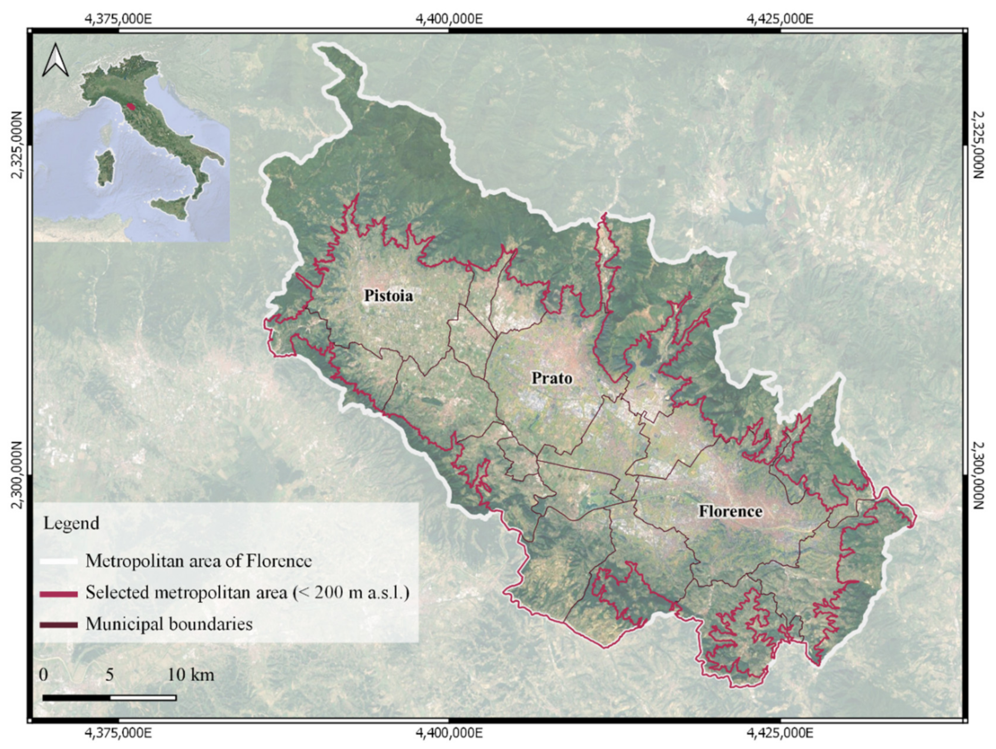
The overall design of the study is based on the following workflow (Figure 1).

The methodology is structured as follows. Section 2.1 briefly describes the study-area. Section 2.2 concerns daytime summer LST and derivate layers analysis, based on Landsat 8 remote sensing data. Section 2.3 is focused on thermal hot-spot detection performed by using Getis-ord Gi* statistics for each value in LST datasets. Adjacent features returning the highest or lowest values within Gi* statistics were considered statistically significant hot/cool-spot areas. Subsequently, Section 2.4 reports the characterization of hot- and cool-spot areas on the basis of a large dataset, defined in the study as “urban features layers”: Normalized Difference Vegetation Index, tree cover, water bodies, impervious surface, albedo, surface area, Shape Index, Sky View Factor, theoretical solar radiation, and population density. Finally, Section 2.5 is related to the description of thermal hot-spot statistical analyses. All outcome layers (raster data) were projected in ETRS89-extendend/LAEA Europe coordinate system.

In this study the underlying assumption is that summer hot-spots are originated by a local combination of multiple urban features layers. For this reason, the contributions of any urban elements (vegetation and water bodies, urban surfaces, morphology, atmospheric, and demographic characteristics) that could exacerbate or mitigate urban thermal conditions during summer diurnal times, were quantified probabilistically by using a logistic modeling approach.

Dominance analysis [41] was used to evaluate the relative importance of predictors by using logistic generalized linear models and thus comparing the set of urban features variables used as predictors in hot-spot models. The importance of a predictor variable to a given model was measured as the increase in the model’s ability to explain the linear variability of the outcomes when a single predictor was added.

2.1. The Study-Area

This study was conducted on the metropolitan area of Florence, located in central Italy, the northern part of the Tuscany Region. The area includes 20 municipalities belonging to the administrative units of three main cities, i.e., Florence, Prato, and Pistoia (Figure 2).

A first criterion to delimitate the investigated metropolitan area was based on the elevation, in this way avoiding biases linked to the topographical lapse rate of LST. A maximum elevation value of 200 m a.s.l. was adopted to focus the analysis only on the densely urbanized plain area. The considered metropolitan area is about 674.90 km², with latitudinal and longitudinal ranges varying from 43°39′25″N to 43°59′53″N and from 10°48′28″E to 11°24′57″E. The average topographic slope is about 10% and the area has a prevailing southern exposure. The most important water elements are the Arno river and its tributaries the Greve and Bisenzio.

According to the Köppen–Geiger climate classification [42], the metropolitan area of Florence has a borderline Mediterranean (Csa) and Humid subtropical climate (Cfa), with a moderate influence of the sea and warm summers.

Geographical and demographic characteristics of the study area are described in Table S1 in the Supplementary Materials. The area has a total of about 1 million inhabitants located in twenty municipalities and Florence, Prato, and Pistoia are among the five most populated cities in Tuscany (source: Italian National Institute of Statistics, ISTAT, https://www.istat.it/en/).

The metropolitan plain represents the most important settlement area of Tuscany, densely inhabited and influenced by strong human pressures. As recognized by the last Regional Landscape Plan of Tuscany [43] the metropolitan area is characterized by territorial fragmentation and a high concentration of residential, commercial, and industrial zones and road infrastructures. It is also affected by wetlands and natural areas, enclosed by highly anthropized zones. These characteristics are expected to decrease the amount of agricultural land, with the loss of agroecosystems, wetlands, and alteration of the riparian vegetation. Data from the Italian National Institute of Environmental Protection and Research (ISPRA) show a percentage of Tuscany soil consumption in 2019 equal to 6.15%, compared to 7.10% national average value [4]. Florence is recognized for a high degree of imperviousness with 41.70% of soil consumption (4267 ha) in 2019.

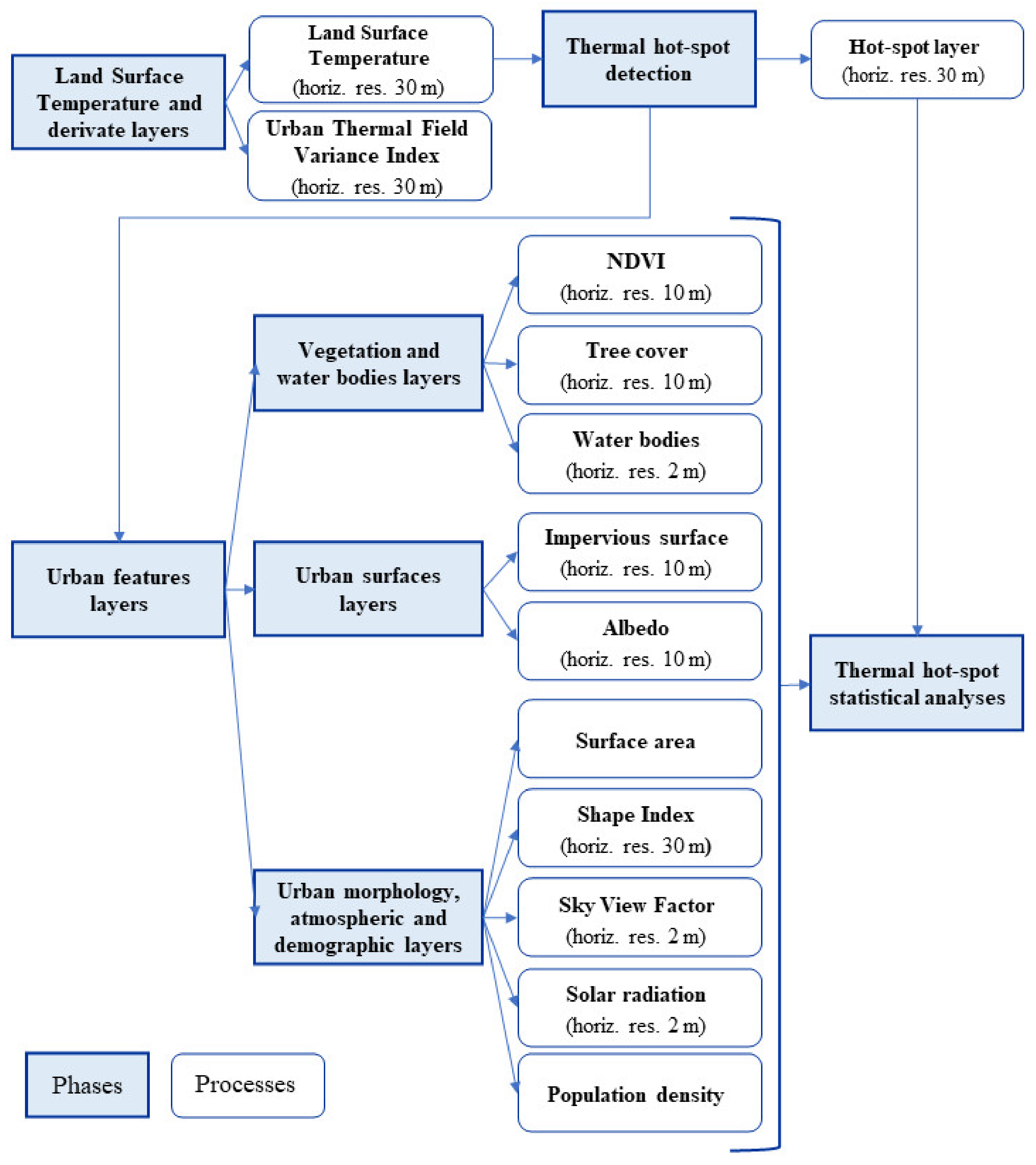
2.2. Land Surface Temperature (LST) and Derivate Layers

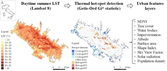
2.2.1. Daytime Summer Land Surface Temperature (LST) Layer

Land Surface Temperature (LST) is an important geophysical parameter of surface energy balance, used to monitor surface thermal processes [38,44,45]. The LST layer in this study was obtained by using Landsat 8 TIRS (Thermal Infrared Sensor) remote sensing data products from the U.S. Geological Survey [46] (https://earthexplorer.usgs.gov), referred to the summer season (from June to August) for the period 2015–2019.

LST was calculated from clear-sky images at 30 m horizontal resolution (the 100 m original resolution of TIRS bands was resampled to 30 m by the U. S. Geological Survey) for daytime (09:58 UTC). Landsat 8 data scene details are reported in Table S2 in the Supplementary Materials. Fourteen scenes (path 192, row 30) covering all the hottest summer months were used by selecting three scenes per year, except for 2018 (that had two scenes). The maximum arbitrary cloud cover threshold adopted in this study to ensure image reliability was less than 3.5%.

LST retrieval was based on the official methodology provided by the U.S. Geological Survey [46] and it was performed using the open source R software [47]. The method involved the conversion of DN (digital number) values of the thermal band (band 10) into top of atmosphere spectral radiance values (TOA), by using the bandwidth-specific factors from the metadata:

TOA = M_L Q_cal + A_L,

(1)

where M_L (3.34 × 10⁻⁴) is band-specific multiplicative rescaling factor; Q_cal is quantized and calibrated standard product pixel values (DN); A_L (0.10) is band-specific additive rescaling factor. Spectral radiance values were used to estimate the top of atmosphere brightness temperature (Tb):

Tb = K₂/ln [(K₁/TOA) + 1],

(2)

where K₁ (774.88) and K₂ (1321.07) are band-specific thermal conversion constants. Surface emissivity (ε) was calculated by adopting the NDVI method [48] on bands 4 and 5. These two bands were previously atmospherically corrected in QGIS Semi-Automatic Classification Plugin [49]. As confirmed by Sekertekin and Bonafoni [50], the land surface emissivity model of Sobrino et al. [48] provides the best performance on all LST retrieval methods, with a low root mean square error value (2.52 K). Finally, LST was extracted as follows:

LST (K) = Tb/[1 + (λ Tb/c₂) ln(ε)],

(3)

where λ is the wavelength of emitted radiance (10.8 µm); and c₂ is obtained by the following equation:

c₂ = h × c/s = 14,388 µm K,

(4)

where h is Planck’s constant (6.626 × 10⁻³⁴ J s); c is the speed of light (2.998 × 10⁸ m/s); and s is Boltzmann constant (1.38 × 10⁻²³ J K⁻¹).

Mean summer daytime LST was calculated by using all available images converted from Kelvin to Celsius degrees (°C).

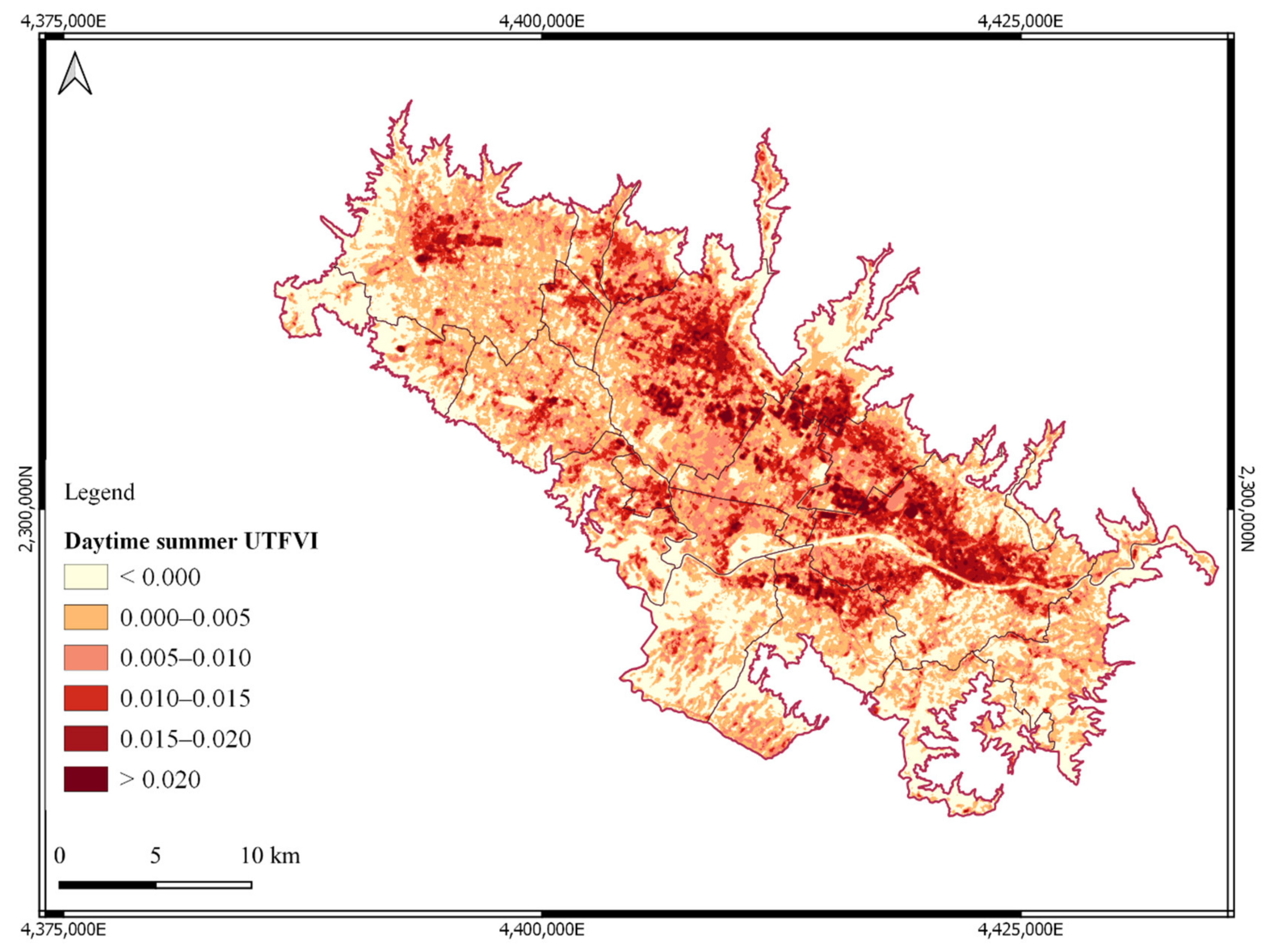
2.2.2. The Urban Thermal Field Variance Index (UTFVI) Layer

Following the estimation of LST, the Urban Thermal Field Variance Index (UTFVI) was selected to apply an ecological evaluation of summer daytime surfaces determined by thermal conditions. Several recent studies used this index to evaluate the SUHI impacts on the quality of urban life [36,51,52]. UTFVI was used to quantitatively describe the SUHI effect and was estimated by the following equation:

UTFVI = (LST − LST_mean)/LST_mean,

(5)

where LST is the surface temperature of a certain point, recorded for each pixel in the daytime summer period 2015–2019 (described in Section 2.2.1) and LST_mean is the average value of the whole study area extracted as raster statistics in QGIS (32.6 °C). UTFVI was calculated by using raster calculator in QGIS environment. Six ecological evaluation thresholds were identified in association with the severity of SUHI phenomenon [51]:

• UTFVI < 0.000 (“excellent”) and absent SUHI;
• UTFVI between 0.000 and 0.005 (“good”) and weak SUHI;
• UTFVI between 0.005 and 0.010 (“normal”) and moderate SUHI;
• UTFVI between 0.010 and 0.015 (“bad”) and strong SUHI;
• UTFVI between 0.015 and 0.020 (“worse”) and stronger SUHI;
• UFTVI > 0.020 (“worst”) and strongest SUHI.

In this study, adverse ecological conditions were defined for UTFVI ≥ 0.010 (from “bad” to “worst”) while all the other situations were defined as favorable ecological conditions (from “excellent” to “normal”).

2.3. Thermal Hot-Spot Detection

The hot-spot analysis conducted in this study was addressed to detect urban areas with daytime LST values showing spatially widespread LST values and thus creating positive or negative structural LST anomalies. Getis-Ord Gi* statistic is the method used to identify statistically significant spatial clusters of high (hot-spots) and low LST values (cool-spots) at local scale.

The criterion for identifying a statistically significant hot-spot (or cool-spot) is that the feature/area should have the highest (or lowest) value, while being surrounded by other features/areas with similar LST values [25]. The analyses for this study were conducted using the Hot-Spot Analysis tool (Getis-Ord Gi*) available in ArcGIS ESRI environment [53]. The method was performed on the averages of daytime summer LST dataset from Landsat 8 imageries, previously converted to a spatial point object. Considering the Landsat 8 resampling carried out by USGS (30 m spatial resolution), the horizontal distance of each LST point object was 30 m. Getis-Ord Gi* statistic method was focused on the calculation for each LST point taken in the context of neighboring points.

The final outputs provided by the Hot-Spot Analysis tool were the significant hot- and cool-spot areas, spatially defined by the following formula [25]:

$${\mathrm{Gi}}^{*}=\frac{{{\displaystyle \sum }}_{\mathrm{j}=1}^{\mathrm{n}}{\mathrm{w}}_{\mathrm{i},\mathrm{j}}{\mathrm{x}}_{\mathrm{j}}-\overline{\mathrm{X}}{{\displaystyle \sum }}_{\mathrm{j}=1}^{\mathrm{n}}{\mathrm{w}}_{\mathrm{i},\mathrm{j}}}{\mathrm{S}\sqrt{\frac{\left[\mathrm{n}{{\displaystyle \sum }}_{\mathrm{j}=1}^{\mathrm{n}}{\mathrm{w}}_{\mathrm{i},\mathrm{j}}^2-{\left({{\displaystyle \sum }}_{\mathrm{j}=1}^{\mathrm{n}}{\mathrm{w}}_{\mathrm{i},\mathrm{j}}\right)}^2\right]}{\mathrm{n}-1}}},$$

(6)

where x_j is the attribute value for feature j; w_i,j is the spatial weight between feature i and j; n is equal to the total number of features.

$\overline{\mathrm{X}}$ and S are mean and variance values, respectively:

$$\overline{\mathrm{X}}=\frac{{{\displaystyle \sum }}_{\mathrm{j}=1}^{\mathrm{n}}{\mathrm{x}}_{\mathrm{j}}}{\mathrm{n}}$$

(7)

$$\mathrm{S}=\sqrt{\frac{{{\displaystyle \sum }}_{\mathrm{j}=1}^{\mathrm{n}}{\mathrm{x}}_{\mathrm{j}}^2}{\mathrm{n}}-{\left(\overline{\mathrm{X}}\right)}^2}$$

(8)

Getis-Ord Gi* application performed in GIS environment requires an appropriate bandwidth to be selected (expressed in meters) in order to perform a reliable hot-spot analysis.

The methodological approach suggests the use of metrics such as inverse Euclidean distance and neighbor maximum distance by considering only the eight neighboring pixels [33]. This approach was applied in the present study for hot-spot detection and the corresponding bandwidth value was about 42.43 m.

The output of the Gi* statistic also provides measures of statistical significance for each feature/area: the probability (Gi* p-value) and standard deviation (Gi* z-score) values. Gi* z-score is a measure of how much the features/areas are clustered, and the Gi* p-value is the probability that the hot-spot patterns found are only due to a random spatial process.

Strictly speaking, a high z-score and a low p-value indicates a significant hot-spot. A low negative z-score and a small p-value indicates a significant cool-spot. The higher (or lower) the z-score, the more intense is the clustering. Thus, three macro groups of thermal patterns were identified:

• cool-spot: statistically significant clustering of low LST values (Gi* z-score < −1.65);
• hot-spot: statistically significant clustering of high LST values (Gi* z-score > 1.65);
• other areas with no significant spatial correlation (−1.65 < Gi* z-score < 1.65).

Confidence level identifies the statistically significance of hot- and cool-spots at thresholds of 90%, 95% and 99%. Therefore, in the Florentine metropolitan area, hot-spots were categorized by 3 × 2 progressive groups based on confidence level thresholds [31]: “Cool-spot99 (cool-spot LEVEL-3)”, “Cool-spot95 (cool-spot LEVEL-2)”, “Cool-spot90 (cool-spot LEVEL-1)”, “Hot-spot90 (hot-spot LEVEL-1)”, “Hot-spot95 (hot-spot LEVEL-2), “Hot-spot99 (hot-spot LEVEL-3)”.

Table 1. Hot-spot classification by applying Getis-Ord Gi* approach.

Gi* Hot-Spot Classes	Confidence Levels	Probability (Gi* p-Value)	Standard Deviation (Gi* z-Score)
Cool-spot99 (LEVEL-3)	99%	<0.01	<−2.58
Cool-spot95 (LEVEL-2)	95%	<0.05	<−1.96
Cool-spot90 (LEVEL-1)	90%	<0.10	<−1.65
Other areas	Not significant	0	−1.65 < z-score < 1.65
Hot-spot90 (LEVEL-1)	90%	<0.10	>1.65
Hot-spot95 (LEVEL-2)	95%	<0.05	>1.96
Hot-spot99 (LEVEL-3)	99%	<0.01	>2.58

shows the hot- and cool-spot classification based on Getis-Ord Gi* approach.

The highest standard deviation (Gi* z-score > 2.58 or Gi* z-score < −2.58) and the lowest probability (Gi* p-value < 0.01) classes defined areas with extreme values (LEVEL-3) where the highest or lowest LST values were clustered with 99% confidence level.

An Inverse Distance Weighted (IDW) interpolation technique was applied on the Getis-Ord Gi* resulting points maps, in this way obtaining hot- and cool-spot raster maps with Landsat 8 grid resolution. This method is suitable to interpolate a raster surface from dense data by using a specific search radius [54]. These outputs were vectorized to obtain hot- and cool-spots as a polygonal feature layer.

2.4. Urban Feature Layers

2.4.1. Vegetation and Water Bodies Layers

Normalized Difference Vegetation Index (NDVI)

Normalized Difference Vegetation Index (NDVI) is one of the most widely applied vegetation indices and an important descriptor of greenness of the biomes. NDVI is considered as land use land cover indicator to quantitatively explore the relationship between the thermal environment and urban expansion [55,56], and to investigate the greening effect on LST changes [32,35,36].

In this study, NDVI is derived from Copernicus Sentinel-2 level-2A raster products by using high-resolution (10 m) remote sensing imagery of the summer daytime period (June to August) in the year 2017. The index was calculated from the reflectance in the red (RED) and near-infrared (NIR) portions of the electromagnetic spectrum, as shown by the following equation:

$$\mathrm{NDVI}=\frac{\mathrm{NIR}-\mathrm{RED}}{\mathrm{NIR}+\mathrm{RED}},$$

(9)

where NIR and RED are band 8 and band 4, respectively.

Theoretically, NDVI values are represented as a ratio ranging from −1 to +1, where positive values indicate vegetated areas and negative values denote non-vegetated areas or vegetation affected by stress. NDVI values are influenced by several factors (vegetation phenology, climatic conditions, water availability) and thresholds may differ by locations and time of the year [57].

Four NDVI thresholds for surface types are generally recognized: NDVI ≤ −0.20 for water, from −0.20 ≤ NDVI < 0.20 for impervious, 0.20 ≤ NDVI < 0.60 for non-irrigated pervious and NDVI ≥ 0.60 for irrigated pervious surfaces. The rationale of the index is that healthy vegetation has a high reflectance in the near-infrared and a low reflectance in the red band, thereby enhancing the interpretation of vegetation cover while suppressing subtle noise from other land cover types.

Tree Cover

Tree cover layer was developed by ISPRA, in the framework of the project “ASI Habitat Mapping” with the purpose of producing a high-resolution (10 m) land cover map of Italy.

In this study, the tree cover was mapped on satellite images of Copernicus Sentinel-1 and Sentinel-2 related to the summer of 2017, in Google Earth Engine environment. The methodology was based on NDVI calculation and the evaluation of thresholds applied on multitemporal remote sensing imagery. The final output is the tree cover binary raster layer (where 0 and 1 are non-tree cover and tree cover surfaces respectively) at 10-m spatial resolution for the summer of 2017. Further information on the workflow methodology is available in Morabito et al. [11].

Water Bodies

Water bodies (rivers, ponds, wetlands, and any other open water) were extracted from the Regional Land Use and Land Cover map (vector data) at scale 1:10,000 for the year 2016, produced by the Environmental Modelling and Monitoring Laboratory for Sustainable Development, LaMMA Consortium (http://www.lamma.rete.toscana.it/). The final output is the water bodies binary raster layer (assuming 1 if water elements were present, or 0 if they were absent) and 2 m horizontal resolution was selected as the maximum threshold in order to spatially combine this data with the other feature layers.

2.4.2. Urban Surfaces Layers

Impervious Surface

Impervious surfaces were detected through a high-resolution (10 m) raster layer for the year 2017, provided by ISPRA. The original data is freely available for the entire Italian territory at National Environmental Information System Network website [58]. These data were produced through a semi-automatic classification methodology that allowed to detect consumed land, and the map is updated every year through the photointerpretation of changes [4,59]. Therefore, impervious areas include buildings, road and railway infrastructure, impervious non-built areas and sports fields, construction sites, permanent greenhouses, mining areas, landfills, and other infrastructure. Further information on the applied methodology is available in the latest report “Land consumption, Land Cover Changes, and Ecosystem Services” published by ISPRA [4] and in other publications [11,40,60].

Albedo

Albedo is the fraction of solar radiation reflected by a surface, depending on various artificial or natural features, including material, color, type of soil, tillage, water content, age of residue [61]. Surface albedo plays an important role in the thermal urban environment and is considered one of the most influencing parameters on the radiation balance of the land surface [62,63].

Albedo values are expressed in a range between 0 (no reflection) and 1 (maximum reflection, typical of a perfectly white surface). Many studies estimated the main typical values of albedo for a variety of natural and artificial surfaces: such as for deciduous forest with leaves (0.18), coniferous forest (0.16), bare soil (dry 0.12, wet 0.15) [61], grass (0.25), water surfaces in relation to different values of solar altitude (y_s) (0.05 for y_s > 45°, 0.08 for y_s = 30°, 0.12 for y_s = 20°, 0.22 for y_s = 10°), asphalt (0.15), and concrete (new 0.55, aged 0.20) [64].

In this study surface broadband albedo (α) was estimated from the Sentinel-2 Level-2A raster products of the 2017 daytime (from 10:00 to 11:00 UTC) summer period by integration of narrowband reflectance across the shortwave spectrum. The following formulas were adopted to obtain a surface albedo map, considering the observed surface as Lambertian [63,65]:

$$\mathsf{\alpha }={{\displaystyle \sum }}_{\mathrm{B}=1}^{\mathrm{N}}{\mathrm{p}}_{\mathrm{B}}\times {\mathrm{w}}_{\mathrm{B}},$$

(10)

$${\mathrm{w}}_{\mathrm{B}}=\frac{{{\displaystyle \int }}_{{\mathrm{L}}_{\mathrm{B}}}^{{\mathrm{H}}_{\mathrm{B}}}{\mathrm{R}}_{\mathrm{s}\mathsf{\lambda }}\times {\mathrm{d}}_{\mathsf{\lambda }}}{{{\displaystyle \int }}_{0.3}^3{\mathrm{R}}_{\mathrm{s}\mathsf{\lambda }}\times {\mathrm{d}}_{\mathsf{\lambda }}},$$

(11)

where p_B is the surface reflectance for a specific band B; w_B is the weighting coefficient; R_sλ is the extraterrestrial solar radiation for the wavelength; d_λ is the bandwidth; L_B and H_B are the lowest and the highest wavelength limits assigned to Sentinel-2 bands. These equations were applied on the VNIR (B2, B3, B4 and B8) and SWIR (B11 and B12) bands. The SWIR bands, with the original 20-m pixel size, were resampled at 10 m in order to obtain a more resolute albedo map, also consistent with the other urban surface layers.

2.4.3. Urban Morphology, Atmospheric and Demographic Layers

Hot-Spot Surface Area and Shape Index (SI)

Hot-spot surface areas were calculated for each hot- and cool-spot category (LEVEL-1, 2, and 3, respectively, for hot- and cold-spot areas). Shape is also an important parameter for urban thermal analysis as the relationship existing between city size, urban form, and the magnitude of the SUHI it produces, has been demonstrated [66]. The Shape Index (SI) is an areal shape metric based on perimeter-area relationships and measures the complexity of a patch compared to a standard shape (squares for raster data, circles for vector data) of the same size [67]. Initially proposed as a diversity index in landscape ecological studies [68], SI is defined as the ratio between patch perimeter and the square root of patch area (m²), adjusted by a constant to account for a square standard [69]:

$$\mathrm{SHAPE}=\frac{0.25{\mathrm{p}}_{\mathrm{ij}}}{\sqrt{{\mathrm{a}}_{\mathrm{ij}}}},$$

(12)

where p_ij is perimeter (m) of patch ij; a_ij is area (m²) of patch ij.

The index was applied to each individual cool- and hot-spot feature (patch), with the aim of providing a measurement of geometrical complexity of the hot-spot pattern. SI values equal to 1 correspond to square patches and increase without limit as patch shape becomes more irregular. SI was computed by the R environment software using specific R packages: “landscapemetrics” [70] and “landscapetools” [71]. The final output is a raster layer with 30 m horizontal resolution.

Sky View Factor (SVF)

The Sky View Factor (SVF) was used as an indicator to describe the urban geometry. It is a dimensionless parameter that returns, with values between 0 and 1, the degree of exposure of a surface to the celestial vault or portion of sky visible from a given point located at ground level [72]. This factor is influenced by the components of the urban fabric, street furniture and trees: values close to 1 correspond to a large visible portion, while values close to 0 indicate a limited view of the sky. SVF can be classified into four categories [73,74]: SVF < 0.25, dense space; 0.25 < SVF < 0.50, semi-dense space; 0.50 < SVF < 0.75, semi-open space; and SVF > 0.75, open space. Moreover, SVF plays an important role in the description of urban radiation properties: the higher its value, the greater the incidence of direct solar radiation (Jiao et al., 2019). The calculation methodology was introduced by Oke [72] and has been widely developed in urban climatology studies [75,76,77]. For a clearer understanding, the SVF calculation of urban geometry is explained by the following Equation [72]:

SVF = cos (tan⁻¹ (2 × H/W),

(13)

where H is the height of the obstacle and W is the distance between obstacles.

The SVF was calculated using the aspect ratio (H/W) of each outdoor open space of the metropolitan area and considering all the streets as street canyons [76]. The input data is the Digital Surface Model (DSM) raster layer, obtained from airborne LIDAR (Light Detection and Ranging) data of the Tuscany Region and the Italian Ministry of the Environment, where the information on building and terrain vertical elevation is stored in every pixel. DSM layers were collected over the period 2007–2010 from LIDAR point cloud data and are freely available at Regional database of Tuscany (GEOscopio platform, http://www502.regione.toscana.it/geoscopio/cartoteca.html). A unique DSM layer of the metropolitan area was obtained by performing 2-m resampling merging the original LIDAR-derived DSM layers (that have 1 m and 2 m horizontal resolutions) available for the investigated areas. As supported by a recent study [77], the DSM layer resolution is an important parameter.

The SVF map was acquired by SAGA (System for Automated Geoscientific Analyses) environment [78] for each pixel of 2 m size of the DSM, therefore considering all obstacles on the surface and depending on the search radius and number of directions (where hemisphere is dissected). The following two input parameters were used, radius of 100 m and 60 search directions as indicated in previous relevant studies [76,77].

Global Solar Radiation

The term “global solar radiation” refers to the amount of direct and diffuse hourly radiation (Wh/m²) reaching a given surface. Solar radiation was simulated using the Area Solar Radiation tool in ArcGis environment [53] with reference to the daily time frame (24 h) of a specific summer day: the summer solstice (June 21st). The aim was to assess the average exposure to global summer solar radiation, under clear sky conditions. The input data was a DSM raster layer, geometrically resampled from 1 m to 2 m and obtained from the final union of airborne LIDAR-derived DSM layers. The calculation was based on the algorithm initially developed by Rich [79] and later improved by Fu and Rich [80]. The height of the sun was simulated by knowing the latitude and longitude and the height of urban elements, projecting shadows, and thus calculating the potential solar incidence. As for SVF, the radiation model required the setting of the search distance, the number of directions, in addition to the parameters of atmospheric transmissibility and the proportion of global radiation fluxes [81]. The final output is a raster layer with 2 m horizontal resolution.

Population Density

Population density data of the Italian National Institute of Statistics (ISTAT) were used to analyze the population spatial distribution in the Florentine metropolitan area. The dataset is freely available on the GEOscopio Regional web platform and consists of the most recent spatial population density database (vector data), divided into census sections covering the whole Tuscany Region. Population density was analyzed in QGIS environment [82] by filtering data exclusively for the residential housing layer, previously downloaded from the GEOscopio platform. The population density data was converted to a raster layer with 2 m horizontal resolution to spatially matching with the other urban feature layers.

2.5. Methodologies to Perform Thermal Hot-Spot Statistical Analyses

The thermal hot- and cool-spot statistical analyses were conducted to describe all urban features layers, previously analyzed. All statistical analyses were performed using IBM SPSS software [83] and R environment [47]. Maps were provided by using QGIS desktop software [82]. QGIS Field Calculator and Zonal Statistic are the tools used to compute surface areas and extract mean values of urban features layers, respectively. The following data were used to fill hot- and cool-spot polygonal layers: label of Gi* confidence level (CL), mean Normalized Difference Vegetation Index (NDVI), tree cover area (TC), water bodies area (WB), impervious area (IA), mean albedo (ALB), surface area (SA), mean Shape index (SI), mean Sky View Factor (SVF), mean global theoretical solar radiation of June 21st (RJ), and mean population density (PD). By using this data matrix, preliminary non-parametric group wise comparisons were conducted by using the Mann–Whitney [84] and Kruskal–Wallis procedures [85] in IBM SPSS environment [83] to put in evidence the raw differences among confidence level classes. The relationships between urban features layers and hot- and cool-spot status, at various significance levels, were analyzed using logistic Generalized Linear Models (GLMs). The use of LST as predictor was not possible because strong non-linearity existed between LST and urban feature layers and linear modeling assumptions were generally not respected. With the aim of performing logistic GLM modeling, a dummy binary variable “HOTSPOTLEV” was created, where the hot-spot referred to LEVEL-1 was taken as reference and set to 0 value in both cool- and hot-spots. Four logistic GLMs were used:

• “Cool-spot ≥95 model”: where HOTSPOTLEV = 1 for LEVEL-2 (95%) and LEVEL-3 (99%);
• “Cool-spot ≥99 model”: where HOTSPOTLEV = 1 for LEVEL-3 (99%);
• “Hot-spot ≥95 model”: where HOTSPOTLEV = 1 for LEVEL-2 (95%) and LEVEL-3 (99%);
• “Hot-spot ≥99 model”: where HOTSPOTLEV = 1 for LEVEL-3 (99%).

Three R packages were used: “pscl” [86] to perform pseudo R-squared computation; “MASS” [87] to perform AIC backward selection; and finally “dominanceanalysis” [88] to obtain a measure of relative importance in GLMs modeling context.

SVF and RJ variables were excluded from the cool-spot model due to lack of LIDAR-derived DSM: the data were only available for about 34.4% of cool-spot areas. The four GLM predictors were selected using minimal Akaike information criterion (AIC) [89] in a stepwise algorithm [87]. AIC technique has been acknowledged as a useful strategy to select the best variable or models in various situations [90]. The pseudo R-squared value of selected models, the AIC and complete model summaries of selected models were computed. GLMs were definitively performed including the variables with a p-value < 0.05. Finally, a General Dominance Analysis (GDA) [41] was performed on the selected significant variables with the aim of quantifying the singular linear average contribution of each predictor in hot- and cool-spots concerning their respective reference level. Dominance analysis is one of the most successful methods for evaluating predictor importance [91]. It examines the contribution of each predictor to the model’s fit in all subset models by using the change in model fit (i.e., R²) and compares it in a pairwise fashion to the contribution of each of the other predictors [92]. More details on GDA analysis were reported in Luo and Azen [93]. The McFadden’s measure [94] was used as pseudo R-squared in the GDA computation. This dimensionless measure varies between 0 and 1 [95] and has the most intuitively reasonable interpretation as a proportional reduction in error measure [96].

3. Results

3.1. Daytime Summer LST and UTFVI Spatial Variations

The descriptive statistics of averaged values of LST and UTFVI are shown in Table S3 in the Supplementary Materials. The quantitative description of UTFVI coverage area for the 2015–2019 period is shown in

Table 2. Percentage coverage area by Urban Thermal Field Variance Index (UTFVI) classes for the overall metropolitan area and the three largest municipalities.

Study-Areas	UTFVI Coverage Area (km2) (%)
	Excellent <0.000	Good 0.000–0.005	Normal 0.005–0.010	Bad 0.010–0.015	Worse 0.015–0.020	Worst >0.020
Florence	32.4 (33.6)	16.9 (17.6)	17.1 (17.8)	18.5 (19.2)	9.7 (10.1)	1.6 (1.7)
Pistoia	42.4 (47.4)	26.7 (29.8)	13.3 (14.8)	5.4 (6.0)	1.6 (1.8)	0.2 (0.2)
Prato	16.8 (21.2)	17.1 (21.5)	21.4 (26.9)	15.6 (19.6)	7.1 (8.9)	1.5 (1.9)
Metropolitan area	296.8 (44.0)	147.7 (21.9)	119.1 (17.6)	74.9 (11.1)	29.7 (4.4)	6.6 (1.0)

Note: coverage area values are calibrated on raster data. The percentage values are related to each study-area.

for the whole metropolitan area and the three largest cities (Florence, Pistoia, and Prato), and in Table S4 in the Supplementary Materials for the other municipalities.

The spatial representations of LST and UTFVI are shown in Figure 3 and Figure 4.

Florence and Prato are the cities that have shown by far the largest surface area affected by adverse ecological conditions (approximately 30 and 24 km², respectively), covering about 27% and 22% of the whole metropolitan area affected by the same conditions, respectively. Considering the whole metropolitan area, almost 17% of the surface was affected by adverse ecological conditions while the rest revealed favorable ecological conditions (Table 2). In particular, eight municipalities exceeded the metropolitan percentage threshold of adverse conditions in relation to the municipal area: Sesto Fiorentino (38.8%), Florence (31.0%), Poggio a Caiano (30.5%), Prato (30.4%), Montemurlo (28.2%), Campi Bisenzio (25.5%), Calenzano (19.6%), and Agliana (19.0%) (Table 2 and Table S4 in the Supplementary Materials). Conversely, more than half of municipalities showed higher percentage values of favorable conditions than the metropolitan area value. The greatest extension of territory characterized by favorable ecological conditions was observed in Pistoia (82.4 km²), representing almost 15% of the whole metropolitan area covered by the same UTFVI classes.

3.2. Spatial Distribution and LST Variation Among Hot-Spot Classes

Descriptive statistics relating to hot-spots and their spatial representation are shown in

Table 3. Percentage coverage area of Gi* hot-spot classes with relative averaged values of LST.

Study-Areas	Gi* Hot-Spot Classes	SA (km2) (%)	N. Hot-Spot Polygons/SA (n/km2)	LST (°C)
				Mean	Min	Max	Sd
Florence	Total cool-spots	3.2 (3.3)	137.8	27.6	27.0	28.3	0.5
	Cool-spot99 (LEVEL-3)	0.5 (0.5)	22.0	25.3	24.9	26.1	0.3
	Cool-spot95 (LEVEL-2)	1.3 (1.3)	70.8	26.6	26.2	27.3	0.4
	Cool-spot90 (LEVEL-1)	1.4 (1.5)	241.4	27.9	27.2	28.6	0.5
	Other areas	79.4 (82.4)	0	33.4	24.7	39.0	2.3
	Hot-spot90 (LEVEL-1)	8.0 (8.3)	52.6	37.3	36.7	37.8	0.4
	Hot-spot95 (LEVEL-2)	5.0 (5.2)	22.0	38.2	37.6	38.7	0.3
	Hot-spot99 (LEVEL-3)	0.8 (0.8)	25.0	39.9	39.3	40.6	0.3
	Total hot-spots	13.8 (14.3)	39.9	37.6	37	38.1	0.4
Pistoia	Total cool-spots	8.5 (9.5)	169.5	27.3	26.5	28.2	0.6
	Cool-spot99 (LEVEL-3)	2.6 (2.9)	32.7	25.1	24.6	26.1	0.4
	Cool-spot95 (LEVEL-2)	3.9 (4.4)	88.5	26.4	25.6	27.4	0.6
	Cool-spot90 (LEVEL-1)	2.0 (2.2)	505.5	27.8	27.0	28.6	0.7
	Other areas	78.7 (87.9)	0	32.7	22.8	37.8	1.9
	Hot-spot90 (LEVEL-1)	1.5 (1.7)	44.0	37.2	36.6	37.6	0.3
	Hot-spot95 (LEVEL-2)	0.7 (0.8)	24.3	38.1	37.4	38.5	0.3
	Hot-spot99 (LEVEL-3)	0.1 (0.1)	10.0	40.1	39.0	41.0	0.5
	Total hot-spots	2.3 (2.6)	36.5	37.4	36.8	37.8	0.3
Prato	Total cool-spots	2.8 (3.5)	132.1	27.3	26.7	28.1	0.5
	Cool-spot99 (LEVEL-3)	0.7 (0.9)	35.7	25.3	24.9	25.9	0.3
	Cool-spot95 (LEVEL-2)	1.3 (1.6)	54.6	26.6	25.9	27.7	0.6
	Cool-spot90 (LEVEL-1)	0.8 (1.0)	342.5	27.7	27.1	28.5	0.6
	Other areas	66.4 (83.5)	0	34.0	23.4	38.5	2.0
	Hot-spot90 (LEVEL-1)	5.7 (7.2)	69.1	37.4	36.8	37.9	0.4
	Hot-spot95 (LEVEL-2)	4.1 (5.2)	23.9	38.1	37.6	38.6	0.3
	Hot-spot99 (LEVEL-3)	0.5 (0.6)	56.0	39.7	39.3	40.0	0.2
	Total hot-spots	10.3 (13.0)	50.5	37.6	37.0	38.1	0.4
Metropolitan area	Total cool-spots	77.7 (11.5)	134.3	27.4	26.6	28.2	0.6
	Cool-spot99 (LEVEL-3)	25.5 (3.8)	20.2	25.3	24.8	26.1	0.4
	Cool-spot95 (LEVEL-2)	34.3 (5.0)	70.4	26.5	25.8	27.5	0.6
	Cool-spot90 (LEVEL-1)	17.9 (2.7)	419.2	27.8	27.0	28.6	0.7
	Other areas	553.2 (82.0)	0	33.0	22.7	39.6	2.2
	Hot-spot90 (LEVEL-1)	24.2 (3.6)	76.0	37.3	36.7	37.8	0.4
	Hot-spot95 (LEVEL-2)	16.9 (2.5)	22.5	38.2	37.5	38.7	0.4
	Hot-spot99 (LEVEL-3)	2.9 (0.4)	35.9	39.8	39.2	40.4	0.3
	Total hot-spots	44.0 (6.5)	52.8	37.6	36.9	38.1	0.4

Note: Gi* hot spot classes are related to hot-spot detection by using Getis-Ord Gi* method. SA (%) is Gi* hot-spot surface area relative to each study-area. Surface areas are calibrated on vector data. Max: maximum value. Sd: standard deviation.

, Figure 5, and Table S5 in the Supplementary Materials.

The whole metropolitan area is covered by almost 20% of thermal anomalies and cool-spots are almost double the hot-spots: 11.5% of cool-spots with average LST minimum and maximum values ranging from 26.6 °C to 28.2 °C and 6.5% of hot-spot areas with LST values ranging from 36.9 °C to 38.1 °C (Table 3). Almost half of the municipalities exceeded the average metropolitan percentage coverage threshold of cool-spots. Thirty-five percent of municipalities revealed a higher percentage coverage value of hot-spots than the average metropolitan area value.

Considering all the cool- and hot-spots in terms of surface areas in km², the highest values were respectively observed in the municipalities of Lastra a Signa (9.9 km²) (Table S5 in the Supplementary Materials) and Florence (13.8 km²) (Table 3). These latter surface areas represented 12.7% and 31.4% of the respective total cool- and hot-spots area of the whole Florentine metropolitan area.

The total cool-spots revealed a higher value of polygons per km² (134.3 n/km²) than the total hot-spots (52.8 n/km²). The lowest values were observed in LEVEL-3 and LEVEL-2 for cool- and hot-spots, respectively, while the highest values were always observed in LEVEL-1. Both for the whole metropolitan area and the single municipalities, LST variations within the three cool- and hot-spot levels were stable (Table 3): about 1.0 °C LST variation was estimated between the previous and next level. In addition, an increase of about 10 °C was generally observed going from the total average cool-spot to the total average hot-spot classes.

Concerning the overall metropolitan area, a mean LST increase of about 14.5 °C was observed between the most extreme cool- and hot-spot levels (LEVEL-3). Focusing on these two classes, the lowest averaged LST values were observed in cool-spots of Pistoia and Serravalle Pistoiese (about 25 °C), whereas the highest averaged LST values were observed in hot-spots of Serravalle Pistoiese (about 42 °C) (Table 3 and Table S5 in the Supplementary Materials).

3.3. Statistical Analyses on Urban Features

3.3.1. Hot-Spot Statistics

The averaged urban feature values (namely NDVI, TC, WB, IA, ALB, SA, SI, SVF, RJ and PD) for cool- and hot-spot levels in the overall study-area are shown in

Table 4. Averaged values of urban features in cool-spot classes, with the exception of the sum of surface area.

Urban Features	Total Cool-Spots	Cool-Spot90 (LEVEL-1)	Cool-Spot95 (LEVEL-2)	Cool-Spot99 (LEVEL-3)
NDVI (adim.)	0.79 ***	0.77 a	0.84 b	0.91 c
TC (%) (m2)	85.0 *** (6825)	82.8 a (2028)	89.1 b (12,858)	97.0 c (45,676)
WB (%) (m2)	3.5 *** (119)	3.7 a (71)	3.4 b (250)	1.7 a (188)
IA (%) (m2)	5.4 *** (259)	6.0 a (127)	4.5 b (512)	2.7 b (933)
ALB (adim.)	0.16 ***	0.17 a	0.16 b	0.15 c
SA (km2)	77.7 ***	17.9 a	34.3 b	25.5 c
SI (adim.)	1.2 ***	1.1 a	1.3 b	1.4 c
SVF (adim.)	0.69 ***	0.70 a	0.66 b	0.59 c
RJ (Wh/m2)	4505.19 ***	4572.11 a	4330.83 b	4072.41 c
PD (people per km2)	14.0 ***	16.0 a	10.7 b	1.5 a

Note: percentage values are related to cool-spot surface area (SA). NDVI: Normalized Difference Vegetation Index. TC: Tree cover. WB: Water bodies. IA: Impervious area. ALB: Albedo. SI: Shape Index. SVF: Sky View Factor. RJ: Global solar radiation of 21 June. PD: Population density. For Cool-spot SVF and RJ data were available only for about 34.4 % (26.7 km²) of the overall Cool-spot coverage area (77.7 km²). *** p-value < 0.001. Different letters indicate statistically significant differences (p-value < 0.05) between cool-spot levels.

and

Table 5. Averaged values of urban features in hot-spot classes, with the exception of the sum of surface area.

Urban Features	Total Hot-Spots	Hot-Spot90 (LEVEL-1)	Hot-Spot95 (LEVEL-2)	Hot-Spot99 (LEVEL-3)
NDVI (adim.)	0.18 ***	0.20 a	0.14 b	0.06 c
TC (%) (m2)	1.7 *** (90)	2.0 a (92)	0.6 a (104)	<0.1 b (14)
WB (%) (m2)	0.1 (6)	0.2 a (6)	<0.1 a (10)	0
IA (%) (m2)	79.1 *** (16,240)	76.4 a (11,001)	86.6 b (38,100)	97.8 b (24,485)
ALB (adim.)	0.24	0.24 a	0.24 a	0.24 a
SA (km2)	44.0 ***	24.2 a	16.9 b	2.9 b
SI (adim.)	1.3 ***	1.3 a	1.4 b	1.2 b
SVF (adim.)	0.80 **	0.80 a	0.78 b	0.79 ab
RJ (Wh/m2)	5236.5 *	5260.97 a	5235.80 a	5408.18 b
PD (people per km2)	1895.5 ***	1849.5 a	2532.8 b	319.7 c

Note: percentage values are related to hot-spot surface area (SA). NDVI: Normalized Difference Vegetation Index. TC: Tree cover. WB: Water bodies. IA: Impervious area. ALB: Albedo. SI: Shape Index. SVF: Sky View Factor. RJ: Global solar radiation of 21 June. PD: Population density. * p-value < 0.05. ** p-value < 0.01. *** p-value < 0.001. Different letters indicate statistically significant differences (p-value < 0.05) between hot-spot levels.

.

The extreme cool-spot level (LEVEL-3) was characterized by the highest TC, NDVI and SI values and the lowest IA and WB frequencies, SVF, RJ and PD (Table 4). Looking at the variation among the cool-spot levels, significant (p-value < 0.001) increases going from LEVEL-1 to LEVEL-3 were observed for SI (27.3%), NDVI (18.2%) and TC (17.1%). In addition, significant (p-value < 0.001) decreases were observed for PDE (90.6%), IA (55.0%), WB (54.1%), SVF (15.7%), ALB (11.8%) and RJ (10.9%). No progressive trend was estimated for SA, showing the minimum and the maximum values in LEVEL-1 and LEVEL-2, respectively.

The extreme hot-spot level (LEVEL-3) was characterized by the highest IA and RJ, and lowest TC, NDVI values, SA, SI, and PD and the absence of WB (Table 5). Considering the variation among hot-spot levels, significant (p-value < 0.001) decreases going from LEVEL-1 to LEVEL-3 were observed for TC (100.0%), SA (88.0%) and NDVI (70.0%), whereas a significant increase (p-value < 0.001) was only observed for IA (28.0%), with almost 100% of surface area covered by imperviousness in LEVEL-3. Significant variations among hot-spot levels, even if with no progressive trends, were observed for SI and PD (p-value < 0.001), SVF (p-value < 0.01) and RJ (p-value < 0.05). Instead, no significant variations among the hot-spot levels (p-value > 0.05) were observed for WB and ALB.

3.3.2. Dominance Analysis

Selected logistic GLMs summaries and the main results of GDA are shown in

Table 6. Summaries of selected cool-spot logistic Generalized Linear Models.

Cool≥95 Model					Cool≥99 Model
McFadden’s R2 = 0.156 AIC = 10,823					McFadden’s R2 = 0.181 AIC = 867.23
	Coefficients					Coefficients
	Estimate	Std. Error	Z-Value	P-Value		Estimate	Std. Error	Z-Value	P-Value
Intercept	−2.040e+00	2.289e−01	−8.915	***	Intercept	−4.140e+00	+7.634e−01	−5.423	***
NDVI	+2.419e+00	+1.817e−01	+13.316	***	NDVI	+3.470e+00	+7.236e−01	+4.795	***
TC	+1.086e−04	+4.883e−06	+22.241	***	TC	+1.370e−05	+1.649e−06	+8.310	***
WB	+1.854e−04	+4.684e−05	+3.959	***	ALB	−1.796e+01	+3.435e+00	−5.228	***
ALB	−8.096e+00	+9.198e−01	−8.802	***	-	-	-	-	-

Note: McFadden’s R² is McFadden’s pseudo R-squared. Std. error: standard error. Significant codes: *** p-value < 0.001.

and

Table 7. Average contribution by predictor (General Dominance Analysis of selected Cool-spot logistic GLMs).

Cool≥95 Model		Cool≥99 Model
Predictors	Average Contribution	Predictors	Average Contribution
	McFadden’s R2		McFadden’s R2
TC	0.114	TC	0.077
NDVI	0.030	NDVI	0.073
ALB	0.009	ALB	0.032
WB	0.003

for cool-spot models and

Table 8. Summaries of selected hot-spot logistic Generalized Linear Models.

Hot≥95 Model					Hot≥99 Model
McFadden’s R2 = 0.118 AIC = 2154.9					McFadden’s R2 = 0.241 AIC = 663.99
	Coefficients					Coefficients
	Estimate	Std. Error	Z-Value	p-Value		Estimate	Std. Error	Z-Value	p-Value
Intercept	−2.267e+00	+1.004e+00	−2.259	*	Intercept	+2.564e+00	+9.784e-01	+2.620	**
NDVI	−5.319e+00	+6.093e−01	−8.729	***	NDVI	−1.868e+01	+2.050e+00	−9.112	***
TC	−1.703e−03	+3.845e−04	−4.430	***	ALB	−8.452e+00	+2.272e+00	−3.720	***
IA	+1.677e−05	+2.530e−06	+6.628	***	SVF	−1.847e+00	+8.909e−01	−2.073	*
ALB	−5.733e+00	+1.355e+00	−4.230	***	PD	−2.211e−04	+8.611e−05	−2.568	*
SI	−5.265e−01	+1.832e−01	−2.874	**	-	-	-	-	-
SVF	−4.143e+00	+8.676e−01	−4.775	***	-	-	-	-	-
RJ	+1.306e−03	+2.632e04	+4.962	***	-	-	-	-	-
PD	+3.763e−05	+1.762e−05	+2.135	*	-	-	-	-	-

Note: McFadden’s R² is McFadden’s pseudo R-squared. Std. error: standard error. Significant codes: * p-value < 0.05. ** p-value < 0.01. *** p-value < 0.001.

and

Table 9. Average contribution by predictor (General Dominance Analysis of selected Hot-spot logistic GLMs).

Hot≥95 Model		Hot≥99 Model
Predictors	Average Contribution	Predictors	Average Contribution
	McFadden’s R2		McFadden’s R2
NDVI	0.051	NDVI	0.199
SI	0.029	PD	0.029
IA	0.027	ALB	0.008
SVF	0.023	SVF	0.005
RJ	0.015
TC	0.009
ALB	0.004
PD	0.001

for hot-spot models.

In Cool≥95 model (R² = 0.156), NDVI, TC, WB and ALB were highly significant predictors (p-value < 0.001), tagged by positive coefficients except for ALB (Table 6). GDA performance in Cool≥95 model (Table 7) revealed TC as the most relevant predictor (R² = 0.114), followed by NDVI (R² = 0.030) and ALB (R² = 0.009). In Cool≥99 model (McFadden’s R² = 0.181), NDVI, TC, and ALB were identified as highly significant predictors (p-value < 0.001) (Table 6) and the highest average contribution followed what was already shown in the Cool≥95 model (Table 7).

In Hot≥95 model (R² = 0.118), most variables were identified as significant predictors (p-value < 0.05 to p-value < 0.001) (Table 8): IA, RJ (p-value < 0.001) and PD (p-value < 0.05) revealed positive coefficients, while NDVI, TC, ALB, SVF (p-value < 0.001), and SI (p-value < 0.01) showed negative coefficients. NDVI was the most important predictor (R² = 0.051), followed by SI (R² = 0.029), IA (0.027) and the other urban elements indicated in Table 9. Hot≥99 model (R² = 0.241) was characterized by four significant variables (p-value < 0.001 for NDVI and ALB; p-value < 0.01 for SVF and PD) identified by negative coefficients (Table 8). Furthermore, for this model, NDVI was the most important predictor (R² = 0.199), followed by the other three urban elements (Table 9).

4. Discussion

This study, through the use of open data and a robust and replicable methodology, allowed the distribution of summer daytime surface thermal hot- and cool-spots in the Florentine metropolitan area to be quantified and spatially represented, identifying the urban features layers that contribute to thermally characterizing these urban landscapes. In particular, the application of a clear and reproducible procedure (the Getis-Ord Gi* statistic) for urban thermal hot-spot detection based on summer daytime Landsat 8 imageries combined with a parametric hot-spot characterization through local urban features layers (based on open data) provided useful information for planning targeted urban mitigation strategies involving specific urban elements in certain areas of the city.

The correct thermal clusters detection is an important issue in urban thermal studies since LST values of a certain location are not independent but are spatially auto-correlated with those of its neighboring areas because of land surface heat fluxes [97].

The significance of hot-spot detection is its capacity to allow statistically-based estimates of spatial variation in thermal aggregation, identifying significant hot-spots in the LST datasets at local level [28,35].

About 20% of the selected metropolitan area (121.7 km² of SA) was affected by thermal anomalies, i.e., 11.5% by cool-spots and 6.5% by hot-spots. As in Jamei et al. [35], also in this research a remarkable part of the study-area (82.0%) has a random LST distribution. We found that cool-spot areas show a higher degree of fragmentation, more than double with respect to the hot-spot ones, in terms of number of cool- and hot-spot polygons per surface area. This is justified by the fact that the large extent of urban areas characterized by soil consumption creates compact hot-spot areas interrupted by more fragmented cool-spot areas.

The average LST variability of 10 °C observed in this study between hot- and cool-spots is in agreement with previous studies [33] where the authors showed that the average summer LST difference between hot- and cool-spots can reach 9.1 °C. Furthermore, the fact that all twenty municipalities in our study revealed a similar average LST variability and about 14.5 °C between the extreme hot- and cool-spot levels (LEVEL-3) could be explained by the right trade-off between the amount of impervious areas and other urban surface layers, the typical LST-related cooling layers (i.e., blue and green infrastructures) and morphological features.

The strength of our results is determined by the fact that data have been collected in a stable period from morphological, structural, and demographic point of view for the study-area where no major large-scale regeneration interventions were observed.

4.1. The Role of Urban Features on Thermal Pattern

Identification of the dominant LST-related factors minimizing their adverse effects, was recognized as an important challenge by recent studies [35,98]. Extensive research demonstrated that LST is closely linked to many parameters: land-use patterns, land coverage, landscape structures and land-use configuration [99,100]. In particular, a more recent study [20], conducted in four cities of the United States, highlighted the strong influence of NDVI and TC, followed by ALB and WB, on daytime LST. This very interesting result is also confirmed in our study since exactly these four variables were identified as significant predictors in the logistic GLMs cool-spots developed and three of these variables (NDVI, TC and ALB) were found to be significant predictors in the logistic GLMs hot-spots. In addition, Logan et al. [20] also revealed that an increase of vegetation and decrease of impervious surfaces were linked to the greatest daytime LST with about a 15 °C change. This finding was in agreement with the average LST variation between the extreme hot- and cool-spot levels (LEVEL-3) in the Florentine area, where an average difference of 14.5 °C was found.

In this study, the local urban features were considered by using open data, in this way ensuring the reproducibility of the analyses in other urban areas. In order to characterize the urban thermal hot-spot pattern, various urban features data were considered: vegetation and water bodies, urban surfaces, morphological, atmospheric, and demographic characteristics layers. Previous studies [29,34,35] performed a geospatial-based hot-spot analysis by using the combination of urban features such as NDVI and PD, selected as proxies for vegetation density and human activity, respectively. As recently suggested by other authors [33,35], understanding the right trade-off between the amount of different urban elements determining hot-spot areas enabled the development of targeted mitigation strategies to counteract overheating in cities.

Nevertheless, the estimation of urban features’ effects on the surface thermal conditions is a complex challenge and has some limitations, especially if linear regression models are performed [20]. In our case, we are aware that the low pseudo R-squared values (from GDA results) confirmed the difficulty in evaluating linear relationships for clustered hot- and cool-spot areas. However, it must also be considered that our analyses focused on highlighting the different combinations of urban features layers that characterize the hottest or coolest urban areas, thus acting on the extreme classes (hot- and cool-spots) of the overall urban LST-pattern.

Identification of the urban elements that contribute to and characterize the various levels of hot- and cool-spots (obtained by the dominance analysis) represents a great strength in this study. In particular, the results obtained can provide useful information to suggest subsequent intervention addressed to mitigate thermal anomalies in the Florentine metropolitan urban area. We found a greater number of urban elements contributing to characterize hot-spot areas than cool-spot ones, while few variables were needed to characterize extreme hot- and cool-spots levels (LEVEL-3). This result is in good agreement with the findings of Shi et al. [101], who demonstrated that the daytime summer thermal environment in a high-density city in China involved several urban design factors, including sky view factor, surface albedo, vegetation cover ratio, building density, and mean building height. Regarding the cooling effects of open spaces, it was widely demonstrated that blue and green spaces are the main LST-drivers [102], in addition to reflective materials, as capable of increasing the surface albedo [103], as also highlighted in our study.

Vegetation has a key role as a strong modulator for thermal phenomenon [7] favoring a cooling effect especially through the evapotranspiration and the shading effect [5,104]. Literature has widely shown the negative correlation between NDVI and LST [8]. Instead, the ALB–LST relationship is complicated and moderately weak in part because both low and high albedo areas can have either reduced or enhanced daytime LST in some cases [17,105]. This is probably linked to the heterogeneity of urban fabric and the complexity of urban energy fluxes. In addition, a previous study [106] demonstrated that the decreased surface ALB was driven by denser vegetation, highlighting that the relationship between vegetation greenness and surface albedo was stronger for sparse vegetation community than for the dense one. The importance of vegetation was also confirmed in our study, in addition to some surface properties: NDVI and ALB were the common elements of both hot- and cool-spot models contributing to describe their thermal conditions. Significant increases of NDVI and TC values were associated to a decrease of ALB values going from the lowest (LEVEL-1) to the highest (LEVEL-3) cool-spot level. The coolest areas (LEVEL-3) revealed the lowest ALB, probably linked to different and darker tree cover species in the study area. As suggested by literature [61,64], the vegetation shows low albedo values ranging from 0.16 for coniferous forests, 0.18 for deciduous forests to 0.25 for grass land. However, the low albedo of plants and generally vegetation do not contribute to overall warming and LST increase because the excess warmth is offset by evaporative cooling from transpiration.

In hot-spot areas significant decreases of vegetation indices (NDVI and TC) and stable ALB values were observed moving from hot-spot LEVEL-1 to LEVEL-3. The different dynamics observed in hot-spot areas were associated with an almost absolute prevalence of imperviousness in hot-spot LEVEL-3 (IA > 97%, NDVI 0.06 and TC surfaces < 0.1%). On the other hand, the stability of albedo levels was probably related to the characteristics of the surfaces that in these urban areas were uniformly characterized by built-up surfaces. Further insights are certainly needed to better understand the mechanistic pathways associated with the role played by various urban elements.

However, the results provided by this study represent an important source of information for planners and policy-makers to localize mitigation strategies on specific hot- and cool-spots. Our results suggest that interventions on hot-spot areas must be generally able to involve various urban elements, while those on cool-spots or the extreme hot-spot level (hot-spot LEVEL-3) must be more targeted by considering fewer elements.

4.2. Cool-Spot Sites

The cool-spot pattern was characterized by features linked to the vegetation (TC and NDVI), water bodies (WB), and urban surface (ALB). In both cool-spot models, TC, NDVI and ALB were the highly significant predictors, whereas WB was an additional predictor only in the cool-spot≥95 model. Cool-spots had low WB values (3.5%), high vegetation density (NDVI always greater than 0.7 and TC surface above 80%), and an average value of ALB of 0.16, confirming the prevalence of pervious surfaces [57,61]. Concerning the vegetation feature, the highest values were observed in the extreme cool-spot level (LEVEL-3): TC was almost 100% with NDVI close to 0.90.

Previous studies have shown that an increase in vegetation cover helps to mitigate SUHI effects through the direct effect of evapotranspiration and shading [5,104]. The cooling effect of urban vegetation has been consistently demonstrated in several cities over the past twenty years using remote sensing at all scales [107,108,109,110,111], and more specifically the effect of TC on SUHI was clearly demonstrated during daytime summer in ten metropolitan Italian cities [11]. It has become widely accepted that TC has higher cooling effect than grass [111,112]: trees have a more intensive evapotranspiration process than an equivalent area of grass, in addition to the fundamental shading effect.

As stated by Alavipanah et al. [113], the relationship between LST and the proportion of vegetation was non-linear in urban areas, showing lower LST where the proportion of vegetation was between 70% and almost 80% per km². There is a consensus in the scientific literature that the TC cooling effect varied greatly between tree species for several reasons, such as the different physiological traits, foliage density, tree height, and canopy geometry [114,115].

Another interesting aspect is the effect provided by the size and shape of green areas. In a recent study [116] carried out on the city of Arizona (US), the authors concluded that the large green space of an irregular shape improved daytime cooling. A more recent study [117] proposed that when the green areas size was limited (<1 ha), a compact shape (circular or square) would be more effective in LST decreasing, while when the area was large (>1 ha), the complex shape of the blue-green space had a good cooling effect. These findings were in agreement with our results. In particular, in the Florentine metropolitan area, the lowest average summer LST values (about 25 °C) were observed in the cool-spot LEVEL-3: characterized on average by high values of TC ratio (97.0% on the total surface area, corresponding to a size about of 4.6 ha), and a more irregular shape than the other cool-spot levels and hot-spots at the same level.

Our results confirmed the important role provided by TC for summer cool-spots. In addition, also WB revealed a strong cooling effect as confirmed by other studies [16,118], especially during the summer [119]. A study conducted in China stressed the importance of the percentage of WB in maximizing the cooling effect of green spaces [120]. In our study, WB partially characterized the cool-spot pattern since the average WB percentage values were very low (3.5%) compared to the surface area. Regarding the urban surface composition, cool-spots showed relatively low ALB values, lower than 0.20, revealing a value corresponding to the typical reflective power of TC areas [61].

4.3. Hot-Spot Sites

The hot-spot pattern revealed a more complex structure and involved a greater number of urban elements, as compared to the cool-spot one. The level of thermal significance was linked to many urban feature layers considered in this study and, in particular, the vegetation state (NDVI and TC), features of urban surfaces (IA and ALB parameters), urban morphology (SI and SVF), atmospheric (RJ), and demographic (PD) features.

The complex hot-spot pattern could be explained in relation to the combined and interconnected role that different urban features layers play during daytime in the surface energy balance and consequently modify the urban microclimatic conditions. The complexity of urban thermal environment was also confirmed by several studies [20,100,101] mentioned in Section 4.1. However, as seen also for cool-spots, vegetation (the NDVI) and ALB were the urban elements generally identified as significant predictors.

The presence of vegetation was on average very low, as confirmed by NDVI values lower than 0.20, corresponding with the typical values of the impervious surfaces [57], and also a value of TC lower than 2%. Conversely, hot-spots were mostly characterized by high IA values (79.1%) associated with low ALB values (0.24), resulting in a high thermal storage capacity. Indeed, IA, as we expected, is the main driver for LST increases, as confirmed by other studies in Italian cities [11,36,40,60], and high values could have negative impacts on plant diversity and ecosystem services [121]. It has been demonstrated that the combined effect of surface properties and urban geometry mostly influence the urban thermal environment, especially in the surface energy flux distribution [111,122]. Studies on the thermophysical properties of materials have highlighted how different urban elements (building roofs, road paving, green surfaces, and urban forests) can influence the microclimatic conditions of the urban environment as a function of albedo [17,103,123]. Surface characteristics of building materials are clearly important and strongly influence the urban microclimate, i.e., dark-colored surfaces, characteristic of asphalt paving, typically have a low albedo and tend to have greater heat capacity and lower reflectivity, contributing to the SUHI [103,124]. Moreover, LST of urban areas is not only related to the structure and composition of land surfaces, but also to the urban areas shape [66,125]. As suggested by Zhou et al. [66], city size shows a strong influence on UHI intensity. In particular, the larger, more compact, and less dispersed the cities are, the stronger their UHI intensity tends to be. Therefore, in this study SI was considered as an important parameter providing a measure of hot-spots geometrical complexity over the metropolitan area. The SI value of the extreme level (LEVEL-3) was closely related to square or circular geometries, revealing the highest average LST value of the study-area (39.8 °C) associated to a more regular shape than the corresponding cool-spot level, as also confirmed in previous studies [126,127].

Concerning urban morphology, mean SVF equal to 0.80 suggested the predominance of open spaces [73,74], resulting in a high sky exposure and a greater amount of solar radiation (RJ = 5236.5 Wh/m², on average) with respect to the cool-spots (SVF = 0.69 and RJ = 4505.19 Wh/m², on average).

The results of Scarano and Sobrino [128] showed that the LST is strongly related to the solar access of surfaces during the morning period in the Italian city of Bari: surfaces with high ALB values warm more quickly by day, given the absence of building and obstacle shadows. Therefore, high sky exposure and solar radiation could have negative impacts on the urban micro-climate because they increase the need for mechanical cooling and ventilation and subsequently energy consumption [129]. PD also have a strong effect on the thermal environment [66]. The demographic characteristics of the study-area showed about 1896 people per km², linked to greater energy consumptions than those in the cool-spots characterized by a lower density (PD = 14.0 people per km², on average).

We found that the median hot-spot (LEVEL-2) was the most densely populated among hot-spot areas, whereas the hottest hot-spot (LEVEL-3) was the least, because it was prevalently industrial and with few residents. In line with the studies of Yue et al. [126] and Sun et al. [127], the highest average LST of the study-area (39.8 °C) was observed in LEVEL-3 hot spot characterized by a more regular SI (average 1.2).

4.4. Study Limitations

This study has some limitations in terms of data and tools. First of all, due to the limitation of Landsat 8 image acquisition, only imageries around 10:00 a.m. were selected and other daytime periods were not considered. As stated by a recent study [50], the cubic convolution resampling by USGS on TIRS data represents a limitation and, therefore, we are aware that is also affects the point sampling used for the Getis-Ord Gi* statistic. However, because averaged summer LST data were used in this study accounting for spatial clusters of high and low LST values, this kind of bias can be certainly considered limited. In addition, the Italian population density dataset used was not based on the 2015–2019 period data, so this may not exactly coincide with the current demographic characteristics.

Additional approaches can be implemented in this study, such as for surface albedo calculation. The method used in the present study for the surface albedo layer [63] assumed the observed surface as Lambertian and this might be a potential limitation in some instances. Although the Lambertian assumption may fail over different land covers, it can be considered reliable in the following study because the satellite data are acquired near midday (from 10:00 to 11:00 UTC) and during summer when a large solar elevation angle is observed. Generally, no albedo changes for rough surfaces are observed at solar elevation angles greater than 25–30° [130]. In the Florentine metropolitan area during the summer months, at about 10:00, the solar elevation angle is on average above 40°; therefore, the used approach is suitable during the daytime summer period. On the other hand, this approach loses robustness when applied during winter, when lower solar elevation angles are observed [63]. Based on findings provided by another recent study on spatial heterogeneity of LST [8], an additional approach for surface albedo retrieval can be implemented in future studies. This method [131] considered the intrinsic black-sky and white-sky albedo values of the surface derived from Sentinel-2A products and was applied in a recent study [132].

In the present study we used open data of local urban features layers analyzed by using tools often suggested by the recent literature, such as QGIS and the proprietary software ArcGIS. However, a wide range of software and spatial analysis tools can be applied to urban features layers.

Moreover, future studies could apply the hot-spot detection in different seasons to analyze interannual variations. Further investigation on urban thermal environment could consider more detailed features of green infrastructure and urban morphology, such as different vegetation canopies (i.e., grass and shrubs), the size and height of trees and buildings, the street geometry and their orientation.

5. Conclusions

This study provides an important contribution exploring the urban thermal pattern on the Florentine plain area through the recognition of statistically significant summer hot- and cool-spot areas, and also showing a design related to local urban features. This statistical approach provides a robust and effective mapping technique to quantify and represent the LST cluster pattern performed by using open remote sensing data and also sourcing an extensive of the literature focused on urban climate and remote sensing applications. The originality of this study lies precisely in processing LST data obtained from satellite images through the application of a robust and replicable spatial-statistical hot-spot detection methodology (the Getis-Ord Gi* statistic), essential for identifying “urban landscape clouds” characterized by significant surface thermal anomalies. This methodology made it possible to quantify the surface of the Florentine metropolitan area affected by summer daytime thermal anomalies (18%): 6.5% of hot-spots and 11.5% of cold-spots. Furthermore, a higher degree of fragmentation of cool-spot areas, more than double than the hot-spot ones, was observed.

The scientific community [11,20,29,34,35,100,101] is in agreement on applying the urban feature layers analyzed in this work for urban climate studies as they accurately describe the main urban structure and characteristics. In addition, the selected layers are particularly suitable to investigate the urban plain context of hinterland Italian cities. However, in cities with different geographical, morphological and built-up characteristics, also additional urban elements can contribute to a better characterization of thermal hot-spot, such as the distance from wide water bodies or from the sea coast line, slope exposure, and the orientation of street network, to name a few. Understanding the processes underlying hot- and cool-spot detection, combined with an investigation of the various urban surface layers contributing to their formation in different urban contexts, is of importance, especially to mitigate the summer SUHI effect [97].

The results of this study revealed that the complex mosaic of urban features layers favors different configurations and levels of thermal hot- and cool-spot patterns, thus representing key factors of the Florentine metropolitan area landscape. In detail, a greater number of urban elements contributing to characterize hot-spot areas than cool-spot ones were found. The surface heating effects (hot-spots) of the study area depended on several urban feature layers, such as vegetation (NDVI and TC), urban surfaces (IA and ALB), morphology (SI and SVF), and the atmospheric (RJ) and demographic (PD) characteristics. Instead, the surface cooling effects (cool-spots) were more related to a restricted group of urban elements involving vegetation and water bodies layers (NDVI, TC, and WB) and one urban surface layer (ALB). In addition, few variables were needed to characterize extreme hot- and cool-spot areas (LEVEL-3), with NDVI and ALB identified as common elements contributing to describe their thermal conditions. These findings highlighted the importance of urban design based on nature-based solutions [22] and reflective materials [103] to improve the urban thermal conditions and consequently the thermal comfort of urban dwellers. Therefore, the proposed methodology based on an open data chain processing could be considered reliable in terms of its reproducibility in other urban contexts. It can provide a useful support for urban planners and policy makers to localize more targeted thermal hot-spot mitigation strategies addressed to specific urban feature layers.

In particular, the identification of urban elements that characterize thermal hot-spot areas should allow decision makers to locate the best mitigation actions (such as greening and cool materials), aimed at improving the local thermal pattern. Moreover, this work, through the detection of thermal critical areas, provides interesting insights to plan future urban-microclimate-improvement-based physical simulations by using tools such as ENVI-MET at very small scale, in this way allowing a more reliable implementation of urban design.

References

1. Population Division, Department of Economic and Social Affairs, United Nations. World Urbanization Prospects: The 2018 Revision; Population Division, Department of Economic and Social Affairs, United Nations: New York, NY, USA, 2019; ISBN 978-92-1-148319-2. [Google Scholar]
2. European Commission. Guidelines on Best Practice to Limit, Mitigate or Compensate Soil Sealing; Publications Office of the European Union: Luxembourg, 2012; ISBN 978-92-79-26210-4. [Google Scholar] [CrossRef]
3. Eurostat LUCAS Primary Data 2015. Available online: https://ec.europa.eu/eurostat/web/lucas (accessed on 1 December 2020).
4. Munafò, M. (Ed.) Land Consumption, Land Cover Changes, and Ecosystem Services; Report SNPA 15/20; Italian National System for Environmental Protection: Rome, Italy, 2020; ISBN 978-88-448-1013-9.
5. U.S. Environmental Protection Agency. Reducing Urban Heat Islands: Compendium; U.S. Environmental Protection Agency: Washington, DC, USA, 2008. Available online: https://www.epa.gov/heat-islands/heat-island-compendium (accessed on 1 December 2020).
6. Voogt, J.A.; Oke, T.R. Thermal Remote Sensing of Urban Climates. Remote Sens. Environ. 2003, 86, 370–384. [Google Scholar] [CrossRef]
7. Chakraborty, T.; Lee, X. A Simplified Urban-Extent Algorithm to Characterize Surface Urban Heat Islands on a Global Scale and Examine Vegetation Control on Their Spatiotemporal Variability. Int. J. Appl. Earth Obs. Geoinf. 2019, 74, 269–280. [Google Scholar] [CrossRef]
8. Guo, A.; Yang, J.; Sun, W.; Xiao, X.; Xia Cecilia, J.; Jin, C.; Li, X. Impact of Urban Morphology and Landscape Characteristics on Spatiotemporal Heterogeneity of Land Surface Temperature. Sustain. Cities Soc. 2020, 63, 102443. [Google Scholar] [CrossRef]
9. Zhou, D.; Zhao, S.; Liu, S.; Zhang, L.; Zhu, C. Surface Urban Heat Island in China’s 32 Major Cities: Spatial Patterns and Drivers. Remote Sens. Environ. 2014, 152, 51–61. [Google Scholar] [CrossRef]
10. Wang, J.; Huang, B.; Fu, D.; Atkinson, P. Spatiotemporal Variation in Surface Urban Heat Island Intensity and Associated Determinants across Major Chinese Cities. Remote Sens. 2015, 7, 3670–3689. [Google Scholar] [CrossRef] [Green Version]
11. Morabito, M.; Crisci, A.; Guerri, G.; Messeri, A.; Congedo, L.; Munafò, M. Surface Urban Heat Islands in Italian Metropolitan Cities: Tree Cover and Impervious Surface Influences. Sci. Total Environ. 2021, 751, 142334. [Google Scholar] [CrossRef] [PubMed]
12. Du, H.; Wang, D.; Wang, Y.; Zhao, X.; Qin, F.; Jiang, H.; Cai, Y. Influences of Land Cover Types, Meteorological Conditions, Anthropogenic Heat and Urban Area on Surface Urban Heat Island in the Yangtze River Delta Urban Agglomeration. Sci. Total Environ. 2016, 571, 461–470. [Google Scholar] [CrossRef]
13. Oke, T.R. Boundary Layer Climates, 2nd ed.; Wiley and Sons: New York, NY, USA, 1978. [Google Scholar]
14. Ferrini, F.; Fini, A.; Mori, J.; Gori, A. Role of Vegetation as a Mitigating Factor in the Urban Context. Sustainability 2020, 22, 4247. [Google Scholar] [CrossRef]
15. Osborne, P.E.; Alvares-Sanches, T. Quantifying How Landscape Composition and Configuration Affect Urban Land Surface Temperatures Using Machine Learning and Neutral Landscapes. Comput. Environ. Urban Syst. 2019, 76, 80–90. [Google Scholar] [CrossRef]
16. Manteghi, G.; Limit, H.B.; Remaz, D. Water Bodies an Urban Microclimate: A Review. Mod. Appl. Sci. 2015, 9, 1–12. [Google Scholar] [CrossRef] [Green Version]
17. Trlica, A.; Hutyra, L.R.; Schaaf, C.L.; Erb, A.; Wang, J.A. Albedo, Landcover, and Daytime Surface Temperature Variation across an Urbanized Landscape. Earths Future 2017, 5, 1084–1101. [Google Scholar] [CrossRef] [Green Version]
18. Jamei, E.; Rajagopalan, P.; Seyedmahmoudian, M.; Jamei, Y. Review on the Impact of Urban Geometry and Pedestrian Level Greening on Outdoor Thermal Comfort. Renew. Sustain. Energy Rev. 2016, 54, 1002–1017. [Google Scholar] [CrossRef]
19. Musco, F. (Ed.) Counteracting Urban Heat Island Effects in a Global Climate Change Scenario; Springer International Publishing: Cham, Switzerland, 2016; ISBN 978-3-319-10424-9. [Google Scholar]
20. Logan, T.M.; Zaitchik, B.; Guikema, S.; Nisbet, A. Night and Day: The Influence and Relative Importance of Urban Characteristics on Remotely Sensed Land Surface Temperature. Remote Sens. Environ. 2020, 247, 111861. [Google Scholar] [CrossRef]
21. Goddard, M.A.; Dougill, A.J.; Benton, T.G. Scaling up from Gardens: Biodiversity Conservation in Urban Environments. Trends Ecol. Evol. 2010, 25, 90–98. [Google Scholar] [CrossRef] [PubMed]
22. Kabisch, N.; Frantzeskaki, N.; Pauleit, S.; Naumann, S.; Davis, M.; Artmann, M.; Haase, D.; Knapp, S.; Korn, H.; Stadler, J.; et al. Nature-Based Solutions to Climate Change Mitigation and Adaptation in Urban Areas: Perspectives on Indicators, Knowledge Gaps, Barriers, and Opportunities for Action. Ecol. Soc. 2016, 21, 39. [Google Scholar] [CrossRef] [Green Version]
23. Kabisch, N.; Korn, H.; Stadler, J.; Bonn, A. (Eds.) Nature-Based Solutions to Climate Change Adaptation in Urban Areas: Linkages between Science, Policy and Practice; Springer International Publishing: Cham, Switzerland, 2017; ISBN 978-3-319-53750-4. [Google Scholar]
24. Anselin, L. Local Indicators of Spatial Association-LISA. Geogr. Anal. 1995, 27, 93–115. [Google Scholar] [CrossRef]
25. Ord, J.K.; Getis, A. Local Spatial Autocorrelation Statistics: Distributional Issues and an Application. Geogr. Anal. 1995, 27, 286–306. [Google Scholar] [CrossRef]
26. Getis, A.; Lacambra, J.; Mur, J.; Zoller, H.G. (Eds.) Spatial Econometrics and Spatial Statistics; Palgrave Macmillan: London, UK, 2004; ISBN 1-4039-0797-8. [Google Scholar]
27. Wolf, T.; McGregor, G. The Development of a Heat Wave Vulnerability Index for London, United Kingdom. Weather Clim. Extrem. 2013, 1, 59–68. [Google Scholar] [CrossRef] [Green Version]
28. Feyisa, G.L.; Meilby, H.; Jenerette, G.D.; Pauliet, S. Locally Optimized Separability Enhancement Indices for Urban Land Cover Mapping: Exploring Thermal Environmental Consequences of Rapid Urbanization in Addis Ababa, Ethiopia. Remote Sens. Environ. 2016, 175, 14–31. [Google Scholar] [CrossRef]
29. Ren, Y.; Deng, L.-Y.; Zuo, S.-D.; Song, X.-D.; Liao, Y.-L.; Xu, C.-D.; Chen, Q.; Hua, L.-Z.; Li, Z.-W. Quantifying the Influences of Various Ecological Factors on Land Surface Temperature of Urban Forests. Environ. Pollut. 2016, 216, 519–529. [Google Scholar] [CrossRef] [Green Version]
30. Sismanidis, P.; Keramitsoglou, I.; Kiranoudis, C.T. Identifying and Characterizing the Diurnal Evolution of Urban Land Surface Temperature Patterns. In Proceedings of the 2017 Joint Urban Remote Sensing Event (JURSE), Dubai, United Arab Emirates, 6–8 March 2017; pp. 1–4. [Google Scholar] [CrossRef]
31. Tran, D.X.; Pla, F.; Latorre-Charmona, P.; Myint, S.W.; Caetano, M.; Kieu, H.V. Characterizing the Relationship between Land Use Land Cover Change and Land Surface Temperature. ISPRS J. Photogramm. Remote Sens. 2017, 124, 119–132. [Google Scholar] [CrossRef] [Green Version]
32. Grigoraș, G.; Urițescu, B. Spatial Hotspot Analysis of Bucharest’s Urban Heat Island (UHI) Using Modis Data. Ann. Valahia Univ. Targoviste Geogr. Ser. 2018, 18, 14–22. [Google Scholar] [CrossRef] [Green Version]
33. Mavrakou, T.; Polydoros, A.; Cartalis, C.; Santamouris, M. Recognition of Thermal Hot and Cold Spots in Urban Areas in Support of Mitigation Plans to Counteract Overheating: Application for Athens. Climate 2018, 6, 16. [Google Scholar] [CrossRef] [Green Version]
34. Ranagalage, M.; Estoque, R.; Zhang, X.; Murayama, Y. Spatial Changes of Urban Heat Island Formation in the Colombo District, Sri Lanka: Implications for Sustainability Planning. Sustainability 2018, 10, 1367. [Google Scholar] [CrossRef] [Green Version]
35. Jamei, Y.; Rajagopalan, P.; Sun, Q. (Chayn) Spatial Structure of Surface Urban Heat Island and Its Relationship with Vegetation and Built-up Areas in Melbourne, Australia. Sci. Total Environ. 2019, 659, 1335–1351. [Google Scholar] [CrossRef] [PubMed]
36. Guha, S.; Govil, H.; Dey, A.; Gill, N. Analytical Study of Land Surface Temperature with NDVI and NDBI Using Landsat 8 OLI and TIRS Data in Florence and Naples City, Italy. Eur. J. Remote Sens. 2018, 51, 667–678. [Google Scholar] [CrossRef]
37. Kaplan, G.; Avdan, U.; Avdan, Z.Y. Urban Heat Island Analysis Using the Landsat 8 Satellite Data: A Case Study in Skopje, Macedonia. Proceedings 2018, 2, 358. [Google Scholar] [CrossRef] [Green Version]
38. Zhou, D.; Xiao, J.; Bonafoni, S.; Berger, C.; Deilami, K.; Zhou, Y.; Frolking, S.; Yao, R.; Qiao, Z.; Sobrino, J.A. Satellite Remote Sensing of Surface Urban Heat Islands: Progress, Challenges, and Perspectives. Remote Sens. 2019, 11, 48. [Google Scholar] [CrossRef] [Green Version]
39. Morabito, M.; Crisci, A.; Gioli, B.; Gualtieri, G.; Toscano, P.; Stefano, V.D.; Orlandini, S.; Gensini, G.F. Urban-Hazard Risk Analysis: Mapping of Heat-Related Risks in the Elderly in Major Italian Cities. PLoS ONE 2015, 10, e0127277. [Google Scholar] [CrossRef] [Green Version]
40. Morabito, M.; Crisci, A.; Messeri, A.; Orlandini, S.; Raschi, A.; Maracchi, G.; Munafò, M. The Impact of Built-up Surfaces on Land Surface Temperatures in Italian Urban Areas. Sci. Total Environ. 2016, 551, 317–326. [Google Scholar] [CrossRef]
41. Budescu, D.V. Dominance Analysis: A New Approach to the Problem of Relative Importance of Predictors in Multiple Regression. Psychol. Bull. 1993, 114, 542–551. [Google Scholar] [CrossRef]
42. Rubel, F.; Kottek, M. Observed and Projected Climate Shifts 1901-2100 Depicted by World Maps of the Köppen-Geiger Climate Classification. Meteorol. Z. 2010, 19, 135–141. [Google Scholar] [CrossRef] [Green Version]
43. Directorate-General of the Government of the Territory of Tuscany Region Territorial, Italian Ministry of Cultural Heritage and Activities and Tourism. “Piano di Indirizzo Territoriale con valenza di Piano Paesaggistico” of Tuscany Region, PIT-PPR. 2015. Available online: https://www.regione.toscana.it/piano-di-indirizzo-territoriale-con-valenza-di-piano-paesaggistico (accessed on 1 December 2020).
44. Zhou, J.; Liang, S.; Cheng, J.; Wang, Y.; Ma, J. The GLASS Land Surface Temperature Product. IEEE J. Sel. Top. Appl. Earth Obs. Remote Sens. 2018, 493–507. [Google Scholar] [CrossRef]
45. Duan, S.-B.; Han, X.-J.; Huang, C.; Li, Z.-L.; Wu, H.; Qian, Y.; Gao, M.; Leng, P. Land Surface Temperature Retrieval from Passive Microwave Satellite Observations: State-of-the-Art and Future Directions. Remote Sens. 2020, 12, 2573. [Google Scholar] [CrossRef]
46. U.S. Geological Survey Landsat 8 (L8). Data Users Handbook. Version 5.0. 2019. Available online: https://www.usgs.gov/media/files/landsat-8-data-users-handbook (accessed on 1 December 2020).
47. R Core Team. R version 3.6.3; The R Foundation for Statistical Computing: Vienna, Austria, 2020; Available online: https://cran.r-project.org/bin/windows/base/old/3.6.3/ (accessed on 1 December 2020).
48. Sobrino, J.A.; Jiménez-Muñoz, J.C.; Paolini, L. Land Surface Temperature Retrieval from LANDSAT TM 5. Remote Sens. Environ. 2004, 90, 434–440. [Google Scholar] [CrossRef]
49. Congedo, L. Semi-Automatic Classification Plugin Documentation; Release 6.4.0.2. Free Software Foundation: Boston, MA, USA, 2020. [CrossRef]
50. Sekertekin, A.; Bonafoni, S. Land Surface Temperature Retrieval from Landsat 5, 7, and 8 over Rural Areas: Assessment of Different Retrieval Algorithms and Emissivity Models and Toolbox Implementation. Remote Sens. 2020, 12, 294. [Google Scholar] [CrossRef] [Green Version]
51. Renard, F.; Alonso, L.; Fitts, Y.; Hadjiosif, A.; Comby, J. Evaluation of the Effect of Urban Redevelopment on Surface Urban Heat Islands. Remote Sens. 2019, 11, 299. [Google Scholar] [CrossRef] [Green Version]
52. Portela, C.I.; Massi, K.G.; Rodrigues, T.; Alcântara, E. Impact of Urban and Industrial Features on Land Surface Temperature: Evidences from Satellite Thermal Indices. Sustain. Cities Soc. 2020, 56, 102100. [Google Scholar] [CrossRef]
53. ESRI ArcGIS Pro Desktop: Release 2.6.0; Environmental Systems Research Institute: Redlands, CA, USA, 2020; Available online: https://desktop.arcgis.com/en/ (accessed on 1 December 2020).
54. Watson, D.F.; Philip, G.M. A Refinement of Inverse Distance Weighted Interpolation. Geoprocessing 1985, 2, 315–327. [Google Scholar]
55. Makinde, O.; Agbor, C. Geoinformatic Assessment of Urban Heat Island and Land Use/Cover Processes: A Case Study from Akure. Environ. Earth Sci. 2019, 78, 12. [Google Scholar] [CrossRef]
56. Nguyen, T.; Lin, T.-H.; Chan, H.-P. The Environmental Effects of Urban Development in Hanoi, Vietnam from Satellite and Meteorological Observations from 1999–2016. Sustainability 2019, 11, 1768. [Google Scholar] [CrossRef] [Green Version]
57. Bartesaghi-Koc, C.; Osmond, P.; Peters, A. Mapping and Classifying Green Infrastructure Typologies for Climate-Related Studies Based on Remote Sensing Data. Urban For. Urban Green. 2019, 37, 154–167. [Google Scholar] [CrossRef]
58. National Environmental Information System Network 2020. National Imperviousness Cartography for the Year 2017. Available online: http://groupware.sinanet.isprambiente.it/uso-copertura-e-consumo-di-suolo/library/consumo-di-suolo/carta-nazionale-consumo-suolo-2017 (accessed on 1 December 2020).
59. Strollo, A.; Smiraglia, D.; Bruno, R.; Assennato, F.; Congedo, L.; De Fioravante, P.; Giuliani, C.; Marinosci, I.; Riitano, N.; Munafò, M. Land Consumption in Italy. J. Maps 2020, 16, 113–123. [Google Scholar] [CrossRef]
60. Morabito, M.; Crisci, A.; Georgiadis, T.; Orlandini, S.; Munafò, M.; Congedo, L.; Rota, P.; Zazzi, M. Urban Imperviousness Effects on Summer Surface Temperatures Nearby Residential Buildings in Different Urban Zones of Parma. Remote Sens. 2018, 10, 17. [Google Scholar] [CrossRef] [Green Version]
61. Hatfield, J.; Sauer, T.; Prueger, J. Radiation Balance. Encycl Soils Environ. 2005, 4, 355–359. [Google Scholar] [CrossRef]
62. Li, H. (Ed.) Pavement Materials for Heat Island Mitigation. Design and Management Strategies; Butterworth-Heinemann: Oxford, UK, 2016; ISBN 978-0-12-803476-7. [Google Scholar] [CrossRef]
63. Bonafoni, S.; Sekertekin, A. Albedo Retrieval from Sentinel-2 by New Narrow-to-Broadband Conversion Coefficients. IEEE Geosci. Remote Sens. Lett. 2020, 17, 1618–1622. [Google Scholar] [CrossRef]
64. Markvart, T.; Castaner, L. (Eds.) Practical Handbook of Photovoltaics Fundamentals and Applications; Elsevier Science Publishers: Amsterdam, The Netherlands, 2003; ISBN 1-85617-390-9. [Google Scholar]
65. Toscano, P. (Ed.) Remote Sensing Applications for Agriculture and Crop Modelling; MDPI—Multidisciplinary Digital Publishing Institute: Basel, Switzerland, 2020; ISBN 978-3-03928-226-5. [Google Scholar]
66. Zhou, B.; Rybski, D.; Kropp, J.P. The Role of City Size and Urban Form in the Surface Urban Heat Island. Sci. Rep. 2017, 7, 4791. [Google Scholar] [CrossRef]
67. McGarigal, K.; Marks, B.J. FRAGSTATS: Spatial Pattern Analysis Program for Quantifying Landscape Structure; Pacific Northwest Research Station, Forest Service, U.S. Department of Agriculture: Corvallis, OR, USA, 1995. [CrossRef]
68. Patton, D.R. A Diversity Index for Quantifying Habitat “Edge”. Wildl. Soc. Bull. 1975, 3, 171–173. [Google Scholar]
69. McGarigal, K.; Cushman, S.A.; Ene, E. FRAGSTATS v4: Spatial Pattern Analysis Program for Categorical and Continuous Maps 2012. Computer software program produced by the authors at the University of Massachusetts, Amherst. 2012. Available online: http://www.umass.edu/landeco/research/fragstats/fragstats.html (accessed on 1 December 2020).
70. Hesselbarth, M.H.K.; Sciaini, M.; With, K.A.; Wiegand, K.; Nowosad, J. Landscapemetrics: An Open-source R Tool to Calculate Landscape Metrics. Ecography 2019, 42, 1648–1657. [Google Scholar] [CrossRef] [Green Version]
71. Sciaini, M.; Fritsch, M.; Scherer, C.; Simpkins, C.E. NLMR and Landscapetools: An Integrated Environment for Simulating and Modifying Neutral Landscape Models in R. Methods Ecol. Evol. 2018, 9, 2240–2248. [Google Scholar] [CrossRef] [Green Version]
72. Oke, T.R. Canyon Geometry and the Nocturnal Urban Heat Island: Comparison of Scale Model and Field Observations. J. Climatol. 1981, 1, 237–254. [Google Scholar] [CrossRef]
73. Svenson, M.K. Sky View Factor Analysis—Implications for Urban Air Temperature Differences. Meteorol. Appl. 2004, 11, 201–211. [Google Scholar] [CrossRef]
74. Baghaeipoor, G.; Nashrollani, N. The Effect of Sky View Factor on Air Temperature in High-Rise Urban Residential Environments. J. Daylighting 2019, 6, 42–51. [Google Scholar] [CrossRef] [Green Version]
75. Hodul, M.; Knudby, A.; Ho, H. Estimation of Continuous Urban Sky View Factor from Landsat Data Using Shadow Detection. Remote Sens. 2016, 8, 568. [Google Scholar] [CrossRef] [Green Version]
76. Bernard, J.; Bocher, E.; Petit, G.; Palominos, S. Sky View Factor Calculation in Urban Context: Computational Performance and Accuracy Analysis of Two Open and Free GIS Tools. Climate 2018, 6, 60. [Google Scholar] [CrossRef] [Green Version]
77. Dirksen, M.; Ronda, R.J.; Theeuwes, N.E.; Pagani, G.A. Sky View Factor Calculations and Its Application in Urban Heat Island Studies. Urban Clim. 2019, 30, 100498. [Google Scholar] [CrossRef]
78. Conrad, O.; Bechtel, B.; Bock, M.; Dietrich, H.; Fischer, E.; Gerlitz, L.; Wehberg, J.; Wichmann, V.; Böhner, J. System for Automated Geoscientific Analyses (SAGA) v. 2.1.4. Geosci. Model Dev. 2015, 8, 1991–2007. [Google Scholar] [CrossRef] [Green Version]
79. Rich, P.M. Characterizing Plant Canopies with Hemispherical Photographs. Remote Sens. Rev. 1990, 5, 13–29. [Google Scholar] [CrossRef]
80. Fu, P.; Rich, P.M. A Geometric Solar Radiation Model with Applications in Agriculture and Forestry. Comput. Electron. Agric. 2002, 37, 25–35. [Google Scholar] [CrossRef]
81. Tiwari, A.; Meir, I.A.; Karnieli, A. Object-Based Image Procedures for Assessing the Solar Energy Photovoltaic Potential of Heterogeneous Rooftops Using Airborne LiDAR and Orthophoto. Remote Sens. 2020, 12, 223. [Google Scholar] [CrossRef] [Green Version]
82. QGIS Development Team QGIS Geographic Information System. Open Source Geospatial Foundation Project. 2020. Available online: http://qgis.osgeo.org (accessed on 1 December 2020).
83. IBM Corp. IBM SPSS Statistic for Windows, Version 27.0; IBM Corp: Armonk, NY, USA, 2019. [Google Scholar]
84. Mann, H.B.; Whitney, D.R. On a Test of Whether One of Two Random Variables Is Stochastically Larger than the Other. Ann. Math. Stat. 1947, 18, 50–60. [Google Scholar] [CrossRef]
85. Kruskal, W.H.; Wallis, W.A. Use of Ranks in One-Criterion Variance Analysis. J. Am. Stat. Assoc. 1952, 47, 583–621. [Google Scholar] [CrossRef]
86. Jackman, S. Pscl: Classes and Methods for R Developed in the Political Science Computational Laboratory, R package version 1.5.5; United States Studies Centre, University of Sydney: Sydney, NSW, Australia, 2020; Available online: https://github.com/atahk/pscl/ (accessed on 10 January 2021).
87. Venables, W.N.; Ripley, B.D. Modern Applied Statistics with S, 4th ed.; Springer: New York, NY, USA, 2002; ISBN 0-387-95457-0. [Google Scholar]
88. Navarrete, C.B.; Soares, F.C. Dominanceanalysis: Dominance Analysis. R Package Version 1.3.0. 2020. Available online: https://CRAN.R-project.org/package=dominanceanalysis (accessed on 1 December 2020).
89. Akaike, H. A New Look at the Statistical Model Identification. IEEE Trans. Automat. Contr. 1974, 19, 716–723. [Google Scholar] [CrossRef]
90. Basak, I. On the Use of Information Criteria in Analytic Hierarchy Process. Eur. J. Oper. Res. 2002, 141, 200–216. [Google Scholar] [CrossRef]
91. Johnson, J.W.; Lebreton, J.M. History and Use of Relative Importance Indices in Organizational Research. Organ. Res. Methods 2004, 7, 238–257. [Google Scholar] [CrossRef]
92. Azen, R.; Traxel, N. Using Dominance Analysis to Determine Predictor Importance in Logistic Regression. J. Educ. Behav. Stat. 2009, 34, 319–347. [Google Scholar] [CrossRef]
93. Luo, W.; Azen, R. Determining Predictor Importance in Hierarchical Linear Models Using Dominance Analysis. J. Educ. Behav. Stat. 2013, 38, 3–31. [Google Scholar] [CrossRef]
94. McFadden, D. The Measurement of Urban Travel Demand. J. Public Econ. 1974, 3, 303–328. [Google Scholar] [CrossRef]
95. Estrella, A. A New Measure of Fit for Equations with Dichotomous Dependent Variables. J. Bus. Econ. Stat. 1998, 16, 198–205. [Google Scholar] [CrossRef]
96. Menard, S. Coefficients of Determination for Multiple Logistic Regression Analysis. Am. Stat. 2000, 54, 17–24. [Google Scholar] [CrossRef]
97. Song, J.; Du, S.; Feng, X.; Guo, L. The Relationships between Landscape Compositions and Land Surface Temperature: Quantifying Their Resolution Sensitivity with Spatial Regression Models. Landsc. Urban Plan. 2014, 123, 145–157. [Google Scholar] [CrossRef]
98. Feng, Y.; Gao, C.; Tong, X.; Chen, S.; Lei, Z.; Wang, J. Spatial Patterns of Land Surface Temperature and Their Influencing Factors: A Case Study in Suzhou, China. Remote Sens. 2019, 11, 182. [Google Scholar] [CrossRef] [Green Version]
99. Fu, P.; Weng, Q. A Time Series Analysis of Urbanization Induced Land Use and Land Cover Change and Its Impact on Land Surface Temperature with Landsat Imagery. Remote Sens. Environ. 2016, 175, 205–214. [Google Scholar] [CrossRef]
100. Zhao, C.; Jensen, J.; Weng, Q.; Weaver, R. A Geographically Weighted Regression Analysis of the Underlying Factors Related to the Surface Urban Heat Island Phenomenon. Remote Sens. 2018, 10, 1428. [Google Scholar] [CrossRef] [Green Version]
101. Shi, Y.; Xiang, Y.; Zhang, Y. Urban Design Factors Influencing Surface Urban Heat Island in the High-Density City of Guangzhou Based on the Local Climate Zone. Sensors 2019, 19, 3459. [Google Scholar] [CrossRef] [Green Version]
102. Antoszewski, P.; Świerk, D.; Krzyżaniak, M. Statistical Review of Quality Parameters of Blue-Green Infrastructure Elements Important in Mitigating the Effect of the Urban Heat Island in the Temperate Climate (C) Zone. Int. J. Environ. Res. Public Health 2020, 17, 7093. [Google Scholar] [CrossRef]
103. Yang, J.; Wang, Z.-H.; Kaloush, K.E. Environmental Impacts of Reflective Materials: Is High Albedo a ‘Silver Bullet’ for Mitigating Urban Heat Island? Renew. Sustain. Energy Rev. 2015, 47, 830–843. [Google Scholar] [CrossRef] [Green Version]
104. Grimmond, C.S.B.; Oke, T.R. An Evapotranspiration-Interception Model for Urban Areas. Water Resour. Res. 1991, 27, 1739–1755. [Google Scholar] [CrossRef]
105. Liu, W.; Feddema, J.; Hu, L.; Zung, A.; Brunsell, N. Seasonal and Diurnal Characteristics of Land Surface Temperature and Major Explanatory Factors in Harris County, Texas. Sustainability 2017, 9, 2324. [Google Scholar] [CrossRef] [Green Version]
106. Tian, L.; Zhang, Y.; Zhu, J. Decreased Surface Albedo Driven by Denser Vegetation on the Tibetan Plateau. Environ. Res. Lett. 2014, 9, 104001. [Google Scholar] [CrossRef]
107. Imhoff, M.L.; Zhang, P.; Wolfe, R.E.; Bounoua, L. Remote Sensing of the Urban Heat Island Effect across Biomes in the Continental USA. Remote Sens. Environ. 2010, 114, 504–513. [Google Scholar] [CrossRef] [Green Version]
108. Mackey, C.W.; Lee, X.; Smith, R.B. Remotely Sensing the Cooling Effects of City Scale Efforts to Reduce Urban Heat Island. Build. Environ. 2012, 49, 348–358. [Google Scholar] [CrossRef]
109. Jenerette, G.D.; Harlan, S.L.; Buyantuev, A.; Stefanov, W.L.; Declet-Barreto, J.; Ruddell, B.L.; Myint, S.W.; Kaplan, S.; Li, X. Micro-Scale Urban Surface Temperatures Are Related to Land-Cover Features and Residential Heat Related Health Impacts in Phoenix, AZ USA. Landsc. Ecol. 2016, 31, 745–760. [Google Scholar] [CrossRef]
110. Yan, H.; Wu, F.; Dong, L. Influence of a Large Urban Park on the Local Urban Thermal Environment. Sci. Total Environ. 2018, 622–623, 882–891. [Google Scholar] [CrossRef]
111. Zhao, J.; Zhao, X.; Liang, S.; Zhou, T.; Du, X.; Xu, P.; Wu, D. Assessing the Thermal Contributions of Urban Land Cover Types. Landsc. Urban Plan. 2020, 204, 103927. [Google Scholar] [CrossRef]
112. Duncan, J.M.A.; Boruff, B.; Saunders, A.; Sun, Q.; Hurley, J.; Amati, M. Turning down the Heat: An Enhanced Understanding of the Relationship between Urban Vegetation and Surface Temperature at the City Scale. Sci. Total Environ. 2019, 656, 118–128. [Google Scholar] [CrossRef]
113. Alavipanah, S.; Wegmann, M.; Qureshi, S.; Weng, Q.; Koellner, T. The Role of Vegetation in Mitigating Urban Land Surface Temperatures: A Case Study of Munich, Germany during the Warm Season. Sustainability 2015, 7, 4689–4706. [Google Scholar] [CrossRef] [Green Version]
114. Shahidan, M.F.; Jones, P.J.; Gwilliam, J.; Salleh, E. An Evaluation of Outdoor and Building Environment Cooling Achieved through Combination Modification of Trees with Ground Materials. Build. Environ. 2012, 58, 245–257. [Google Scholar] [CrossRef]
115. Rahman, M.A.; Armson, D.; Ennos, A.R. A Comparison of the Growth and Cooling Effectiveness of Five Commonly Planted Urban Tree Species. Urban Ecosyst. 2015, 18, 371–389. [Google Scholar] [CrossRef]
116. Li, X.; Kamarianakis, Y.; Ouyang, Y.; Turner II, B.L.; Brazel, A. On the Association between Land System Architecture and Land Surface Temperatures: Evidence from a Desert Metropolis—Phoenix, Arizona, USA. Landsc. Urban Plan. 2017, 163, 107–120. [Google Scholar] [CrossRef] [Green Version]
117. Yang, G.; Yu, Z.; Jørgensen, G.; Vejre, H. How Can Urban Blue-Green Space Be Planned for Climate Adaption in High-Latitude Cities? A Seasonal Perspective. Sustain. Cities Soc. 2020, 53, 101932. [Google Scholar] [CrossRef]
118. Wu, C.; Li, J.; Wang, C.; Song, C.; Chen, Y.; Finka, M.; La Rosa, D. Understanding the Relationship between Urban Blue Infrastructure and Land Surface Temperature. Sci. Total Environ. 2019, 694, 133742. [Google Scholar] [CrossRef] [PubMed]
119. Sun, Y.; Gao, C.; Li, J.; Wang, R.; Liu, J. Quantifying the Effects of Urban Form on Land Surface Temperature in Subtropical High-Density Urban Areas Using Machine Learning. Remote Sens. 2019, 11, 959. [Google Scholar] [CrossRef] [Green Version]
120. Yang, C.; He, X.; Yu, L.; Yang, J.; Yan, F.; Bu, K.; Chang, L.; Zhang, S. The Cooling Effect of Urban Parks and Its Monthly Variations in a Snow Climate City. Remote Sens. 2017, 9, 1066. [Google Scholar] [CrossRef] [Green Version]
121. Yan, Z.; Teng, M.; He, W.; Liu, A.; Li, Y.; Wang, P. Impervious Surface Area Is a Key Predictor for Urban Plant Diversity in a City Undergone Rapid Urbanization. Sci. Total Environ. 2019, 650, 335–342. [Google Scholar] [CrossRef]
122. Daramola, M.T. Analysis of the Urban Surface Thermal Condition Based on Sky-View Factor and Vegetation Cover. Remote Sens. Appl. 2019, 15, 100253. [Google Scholar] [CrossRef]
123. Al-hafiz, B.; Musy, M.; Hasan, T. A Study on the Impact of Changes in the Materials Reflection Coefficient for Achieving Sustainable Urban Design. Procedia Environ. Sci. 2017, 38, 562–570. [Google Scholar] [CrossRef]
124. Mohajerani, A.; Bakaric, J.; Jeffrey-Bailey, T. The Urban Heat Island Effect, Its Causes, and Mitigation, with Reference to the Thermal Properties of Asphalt Concrete. J. Environ. Manag. 2017, 197, 522–538. [Google Scholar] [CrossRef]
125. Yin, C.; Yuan, M.; Lu, Y.; Huang, Y.; Liu, Y. Effects of Urban Form on the Urban Heat Island Effect Based on Spatial Regression Model. Sci. Total Environ. 2018, 634, 696–704. [Google Scholar] [CrossRef]
126. Yue, W.; Liu, Y.; Fan, P.; Ye, X.; Wu, C. Assessing Spatial Pattern of Urban Thermal Environment in Shanghai, China. Stoch. Environ. Res. Risk Assess. 2012, 26, 899–911. [Google Scholar] [CrossRef]
127. Sun, R.; Lü, Y.; Chen, L.; Yang, L.; Chen, A. Assessing the Stability of Annual Temperatures for Different Urban Functional Zones. Build. Environ. 2013, 65, 90–98. [Google Scholar] [CrossRef]
128. Scarano, M.; Sobrino, J.A. On the Relationship between the Sky View Factor and the Land Surface Temperature Derived by Landsat-8 Images in Bari, Italy. Int. J. Remote Sens. 2015, 36, 4820–4835. [Google Scholar] [CrossRef]
129. Zhang, J.; Heng, C.K.; Malone-Lee, L.C.; Hii, D.J.C.; Janssen, P.; Leung, K.S.; Tan, B.K. Evaluating Environmental Implications of Density: A Comparative Case Study on the Relationship between Density, Urban Block Typology and Sky Exposure. Autom. Constr. 2012, 22, 90–101. [Google Scholar] [CrossRef]
130. Cierniewski, J.; Karnieli, A.; Kazmierowski, C.; Krolewicz, S.; Piekarczyk, J.; Lewinska, K.; Goldberg, A.; Wesolowski, R.; Orzechowski, M. Effects of Soil Surface Irregularities on the Diurnal Variation of Soil Broadband Blue-Sky Albedo. IEEE J. Sel. Top. Appl. Earth Obs. Remote Sens. 2015, 8, 493–502. [Google Scholar] [CrossRef]
131. Li, Z.; Erb, A.; Sun, Q.; Liu, Y.; Shuai, Y.; Wang, Z.; Boucher, P.; Schaaf, C. Preliminary Assessment of 20-m Surface Albedo Retrievals from Sentinel-2A Surface Reflectance and MODIS/VIIRS Surface Anisotropy Measures. Remote Sens. Environ. 2018, 217, 352–365. [Google Scholar] [CrossRef]
132. Chakraborty, T.; Hsu, A.; Manya, D.; Sheriff, G. Disproportionately Higher Exposure to Urban Heat in Lower-Income Neighborhoods: A Multi-City Perspective. Environ. Res. Lett. 2019, 14, 105003. [Google Scholar] [CrossRef] [Green Version]
Figure 1. Workflow of data processing.
Remotesensing 13 00538 g001
Figure 2. Geographical location map of the metropolitan area of Florence.
Remotesensing 13 00538 g002
Figure 3. Daytime summer land surface temperature (LST) map (2015–2019).
Remotesensing 13 00538 g003
Figure 4. Daytime summer Urban Thermal Field Variance Index (UTFVI) map (2015–2019).
Remotesensing 13 00538 g004
Figure 5. Hot-spot detected map.
Remotesensing 13 00538 g005