Article

Consistent Long-Term Monthly Coastal Wetland Vegetation Monitoring Using a Virtual Satellite Constellation

1
Department of Civil, Environmental and Construction Engineering, University of Central Florida, Orlando, FL 32816, USA
2
Department of Civil Engineering, Embry-Riddle Aeronautical University, Daytona Beach, FL 32114, USA
*
Author to whom correspondence should be addressed.
Remote Sens. 2021, 13(3), 438; https://doi.org/10.3390/rs13030438
Submission received: 29 November 2020 / Revised: 15 January 2021 / Accepted: 20 January 2021 / Published: 27 January 2021
(This article belongs to the Special Issue Wetland Landscape Change Mapping Using Remote Sensing)

Abstract

:
Long-term monthly coastal wetland vegetation monitoring is the key to quantifying the effects of natural and anthropogenic events, such as severe storms, as well as assessing restoration efforts. Remote sensing data products such as Normalized Difference Vegetation Index (NDVI), alongside emerging data analysis techniques, have enabled broader investigations into their dynamics at monthly to decadal time scales. However, NDVI data suffer from cloud contamination making periods within the time series sparse and often unusable during meteorologically active seasons. This paper proposes a virtual constellation for NDVI consisting of the red and near-infrared bands of Landsat 8 Operational Land Imager, Sentinel-2A Multi-Spectral Instrument, and Advanced Spaceborne Thermal Emission and Reflection Radiometer. The virtual constellation uses time-space-spectrum relationships from 2014 to 2018 and a random forest to produce synthetic NDVI imagery rectified to Landsat 8 format. Over the sample coverage area near Apalachicola, Florida, USA, the synthetic NDVI showed good visual coherence with observed Landsat 8 NDVI. Comparisons between the synthetic and observed NDVI showed Root Mean Squared Error and Coefficient of Determination (R2) values of 0.0020 sr−1 and 0.88, respectively. The results suggest that the virtual constellation was able to mitigate NDVI data loss due to clouds and may have the potential to do the same for other data. The ability to participate in a virtual constellation for a useful end product such as NDVI adds value to existing satellite missions and provides economic justification for future projects.

Graphical Abstract

1. Introduction

High quality satellite imagery available to the public at no cost is a key driver for innovation in the applied earth observation space. In particular, it significantly advances simulated constellations of medium resolution sensor data for monthly monitoring of earth’s coastal and terrestrial systems [1,2]. Coastal wetlands (CW) have been recognized for their ability to enhance water quality, recharge aquifers, stabilize shorelines, provide nurseries for fisheries, and offer a setting for numerous recreational activities [3]. Unfortunately, CW are deteriorating due to climate change, human activity, and accelerating rates of sea level rise [4,5,6]. Considering the extensive protective and non-protective ecosystem services they provide, it is important to monitor and, if necessary, protect and restore these valuable resources.
Satellite remote sensing has many inherent capabilities that make it a strong contributor to investigating and monitoring CW. However, even with high resolution, a single sensor can have limitations in terms of spatio-temporal coverage in a selected scene or series of scenes that hinders continuous long-term CW monitoring. Therefore, multi-sensor fusion plays an important role in aggregating complementary data from multiple sensors [7]. This is especially useful for CW areas where fully intact coverage is difficult for a single sensor due to frequent thick cloud cover [8]. In this regard, a potential problem lies in the synergistic use of multiple satellite systems. Fusion of satellite data from multiple sources involves an inherent disruption of harmonizing information due to differences in ground resolution, spectral ranges, and spectral properties, such as band number, position, and width [9]. Therefore, using satellite sensors of similar spatial and spectral properties, especially for monthly CW analyses, is vital for the coherent fusion of multi-sensor satellite data.
Landsat is generally recognized to have the longest publicly available data record beginning in 1972. Landsat 5 has been producing imagery since 1984 and has been used extensively for local and global monitoring. Landsat 8 (L8), launched in 2013, is the latest generation space vehicle in the Landsat Data Continuity mission. The Operational Land Imager (OLI) and Thermal Infrared Sensor (TIRS) are both currently in operation aboard L8 with an orbital revisit time of 16 days [1]. The historical record of Landsat imagery is hindered by the cloud and shadow obscurity that affects all passive optical satellite sensors. Periods of obscured imagery in the time series record of L8 requires complementary data to make it suitable for monthly CW monitoring in applications such as long-term salt marsh change and mapping [10,11], forest degradation [9], rapid phenology changes [11], and CW degradation [12,13].
Normalized Difference Vegetation Index (NDVI) is calculated from multispectral optical remote sensors and characterizes the reflective and absorptive characteristics of the ground surface in the red and near infrared (NIR) bands. A consistent investigation of NDVI over time at local to regional scales can indicate phenological and event-driven changes in coastal marsh vegetation [11,13,14]. Current optical sensors have enough spatial and temporal resolution for NDVI production, but images may be obscured by clouds thereby masking critical areas of change over time. These obscured pixels are one of the principal barriers to effective satellite image interpretation from optical sensors. However, panchromatic and multispectral sensors such as Landsat, Advanced Spaceborne Thermal Emission and Reflection Radiometer (ASTER), and Sentinel are the only freely available (to the public) sources of reflectance data [15] with others being commercial and not publicly available except at significant cost. Hyperspectral sensors on satellites such as MERIS/ENVISAT-1 could provide additional useful information about the composition of coastal vegetation however their relatively coarse resolution is not suitable for a local ecosystem change identification and the narrow swath width results in low availability of data for coastal areas, both of which prevent their efficient and widespread utilization for many coastal applications.
Previous research has reported many successful applications of sensor fusion among Landsat, Moderate Resolution Imaging Spectroradiometer, (MODIS), and Sentinel [16,17]. Additionally, satellite sensors including Landsat, Advanced Very High Resolution Radiometer (AVHRR), ASTER, Sentinel, and MODIS have been used for NDVI mapping at local or global scales [18,19]. Despite the availability of NDVI data from multiple sources, an inherent inconsistency hinders the synergistic use of multi-source NDVI. Previous researchers such as Fan and Liu [20] have also presented comprehensive literature reviews on spectral consistency issues in NDVI data. Since NDVI is computed using reflectance values in the red and NIR bands, any spectral band inconsistencies directly impact the NDVI calculations. For example, satellite observations are post-processed to rectify various spatial [21], temporal [22], radiometric [23], and spectral factors [24]. Much of this work is focused on facilitating sensor fusion at the surface reflectance level, rather than at the indexed data product level (NDVI for example). Specifically, recent work by Padró et al. fused L8 OLI with Sentinel-2A MultiSpectral Instrument (MSI) surface reflectances to radiometrically correct blue, green, red, NIR, short-wave infrared (SWIR) 1, and SWIR 2 bands [25]. Claverie et al. also harmonized L8 OLI and S2A MSI into a virtual constellation to produce a surface reflectance dataset [26]. While it is crucial to investigate spectral differences, extending the analysis to derived products such as NDVI is important for assessing the applicability of sensor fusion to meet the long term monitoring needs of the scientific community [7,27].
Differences in spatial resolution can add bias to fused NDVI data since it is scale dependent [28]. To reduce overall uncertainty, multiple NDVI intercalibration studies agree that data from the subject and reference sensors must be spatially co-registered and resampled enabling the comparison of data at the pixel level [29]. Subsequently, any physical quantities can be computed via accurate sensor calibration. In cases of spectral and spatial similarity, multi-sensor data can be used interchangeably [1,30]. In other cases, the multi-sensor data are compared prior to being combined [31]. However, research gaps remain in the body of knowledge around sensor fusion.
Flood [32] compared Sentinel-2A (S2A) MSI and L8 OLI data but did not account for mis-registration between sensors. While previous research had focused on terrestrial areas (desert) only [33] and used simulated reflectance data [34], their models considered only limited amounts of data from the spatio-temporal domain. These models were based on the fusion of multi-sensor data for pre-selected dates only, thus rendering the model inapplicable to other seasons [35]. However, Arekhi et al. did investigate sensor fusion across seasons for both individual bands and vegetation indices and concluded that absent systematic errors in data retrieval or random errors in atmospheric interference, L8 OLI and S2A MSI can be used for long term monitoring [36]. Other studies into sensor fusion did not consider more than two satellite systems of similar spectral and spatial features [37] or focused on categorically different land cover types such as urban areas [38].
The aforementioned research gaps are perhaps most prominent in multiple sensor fusion models that are applicable to any season or any area. Therefore, we propose a virtual constellation model for NDVI that integrates compatible sensors and addresses the sensor inequality issues by utilizing the coincident imagery from a selected four-year time series. The technique uses S2A MSI and ASTER synergistically with L8 OLI. The free access to L8, S2A, and ASTER, the similar wavelength for the bands relevant to NDVI, and similar geographic coordinate systems [39] provide a viable opportunity to combine these three satellite systems for more continuous monthly monitoring of CW areas. ASTER has been used in conjunction with Landsat 5 (L5) to compare two vegetation indices generated by these two sensors. Both NDVI and soil-adjusted vegetation index (SAVI) showed lower spectral vegetation index measurements for ASTER compared to L5 Enhanced Thematic Mapper Plus (ETM+) for the same target, but still showed a strong positive linear relationship [40]. Several simulation studies have also shown the potential of combining S2A and L8 [41,42] as well as L8 and ASTER [40]. Here, we build on this previous work to demonstrate the benefit of using of L8, ASTER and S2A synergistically for long term continuous monthly monitoring of NDVI in coastal wetlands.
Pohl and Van Genderen [43], Zhang [44], and Zhu et al. [45] catalogued and reviewed various approaches for satellite image fusion such as intensity-hue-saturation [46], principal component analysis [47], wavelet decomposition [48], high-pass filter (HPF) [49], sparse representation [50] and area-to-point regression kriging (ATPRK) methods [51]. Recently, machine learning techniques such as deep learning [52] and random forest (RF) [53] have gained popularity in satellite image fusion. Considering its advantages and past performance [54], an RF algorithm is proposed here for the multi-sensor data alignment in the virtual constellation of L8, S2A, and ASTER. Our approach for multi-sensor data integration is to first designate the most ubiquitous sensor with the longest data record, in this case L8, as the baseline. The second component of our approach is to investigate baseline and peer sensors for similar spectral features and to develop candidates for multi-sensor inequality alignment and finally fusion. Third, the hierarchical fusion workflow is established to produce enhanced cloud-free NDVI that mimics the L8 product.
There are two sub-approaches for this task. The first is to resample and interpolate the 20 m S2A Level-1C data and the 15 m ASTER Level-1B data to the 30 m spatial resolution of L8 Level-1B. S2A Level-1C top-of-atmosphere (TOA) reflectance is geometrically and radiometrically rectified with orthorectification to generate accurate geolocated products. ASTER Level-1B data contain calibrated at-sensor radiances, which are geometrically corrected and geolocated. The process for resampling is straightforward but effectively discards some of the valuable 20 m information obtained by S2A and 15 m information obtained by ASTER. Since our objective is to enrich the existing L8 with available complementary data, we retained all spatial and spectral characteristics of L8 and modified the other two satellites accordingly. The fusion of L8 with S2A and ASTER data can increase the spatial coverage of data available for continuous monthly monitoring. This is especially beneficial in CW areas where cloud and water vapor mask a high percentage of the data [55]. The second option was to compute NDVI from each sensor first before the co-registration and scaling. This approach is called ‘index then blend (IB)’ [56,57]. The IB approach has been found to be computationally more accurate because it mitigates error propagation compared to the alternative [56].
This paper presents a virtual constellation that integrates NDVI data from three satellite sensors that have similar spectral features: L8, S2A, and ASTER. The combined imagery enables NDVI observations of CW at 30 m spatial resolution similar to L8 with more available spatio-temporal coverage. The novelty in the current study lies in the use of four years of coincident NDVI imagery to train components of the virtual constellation to predict NDVI for any selected date irrespective of season, thus making the model robust and adaptive to seasonal and inter-annual changes. The virtual constellation model will serve as a unique tool for coastal managers to continuously monitor long term CW changes.

2. Materials and Methods

The virtual constellation methodology is divided into three major components: data collection and pre-processing; model development; and model validation. The components are illustrated and explained in detail in this section but first we begin with a description of the research setting.

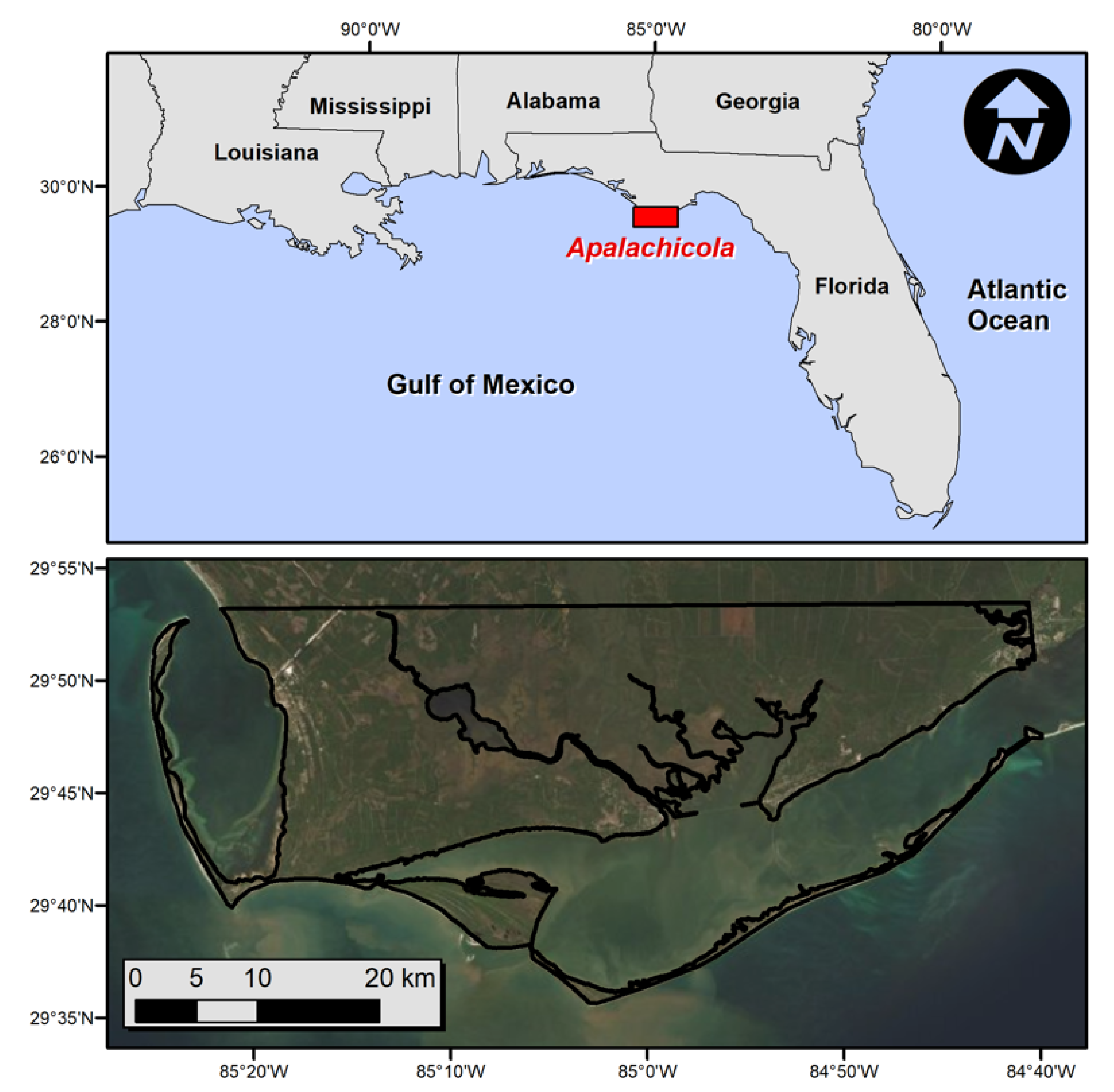
2.1. Research Setting in Apalachicola Bay

We conducted our study in the salt marshes of Apalachicola Bay, located on the Gulf of Mexico coast in the Florida panhandle (Figure 1). The study area occupies a section of the complete L8 Path 19/Row 39 scene, containing a total area of 1053.24 km2. The study site in Apalachicola Bay contains a variety of CW vegetation. The relevant wetland land cover types classified by the National Oceanographic and Atmospheric Administration (NOAA) Coastal Change Analysis Program (C-CAP) [58] in the study area are: 54.1% palustrine forested wetland (PFW), 7.86% palustrine emergent wetland (PEW), 11.66% palustrine scrub and emergent wetlands (PSEW), and 6.48% estuarine emergent wetland (EEW). Estuarine forested wetland and estuarine scrub or shrub wetland are negligible (<1%) in the study area. 19.56% of the study area was made up of developed areas, agricultural use, and bare land [59].
Apalachicola Bay was selected as the research setting because of its location in a sub-tropical coastal area where clouds are frequently present throughout the year and because of the importance of CW to the local economy [13,54,60].

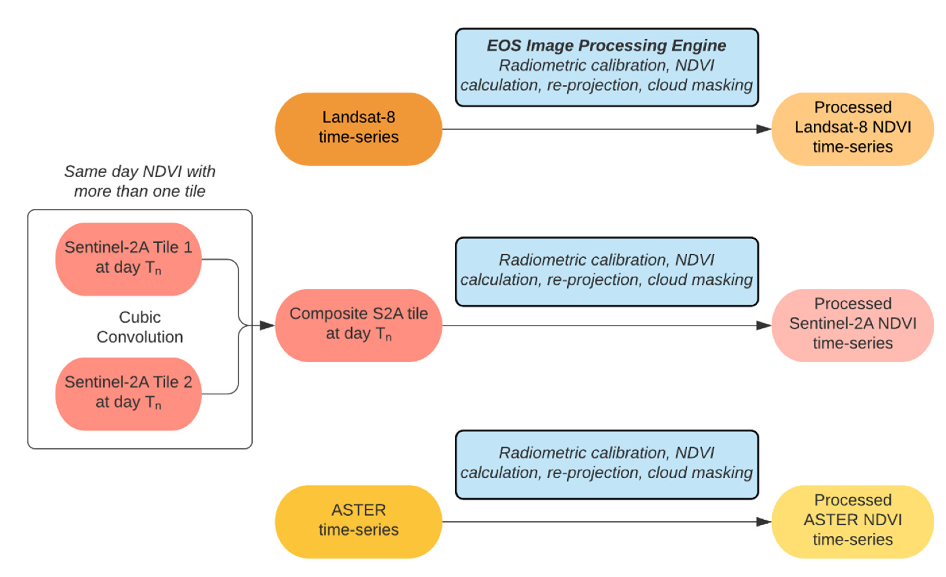
2.2. Sensor Data Collection and Pre-Processing

L8, S2A and ASTER data from the years 2015 through 2018 were collected and processed for the current study (Figure 2). These years represent the time period (ongoing) where data are available for all three sensors.
Landsat 8 (L8) data were collected from the NASA Earth Observing System (EOS) [61], for the years 2015 through 2018. L8 was initially known as the Landsat Data Continuity Mission and was launched on 11 February 2013. Similar to the previous generations of Landsat, L8 has a 16 day repeat cycle. The L8 OLI sensor captures nine spectral bands, including a panchromatic (PAN) band. The visible, near infrared (VNIR) and shortwave infrared (SWIR) bands are produced with a 30 m spatial resolution while the PAN band is produced at 15 m spatial resolution. The L8 swath width is 185 km. We downloaded L8 images covering the Paths 19–20, Row 39. While Path 20, Row-39 covers 100% of our study area, Path 19, Row-39 covers almost 50% of the eastern side of the study area. The reason for keeping two different combinations of Paths and Rows is to accumulate more dates in the temporal domain for training the RF. A sharp edge is observed in the L8 image for the dates where only one pass (Path 19, Row-39) covering approximately half of the study area was available (Figure 3).
We pre-processed the L8 data for years 2015 through 2018 using the analytics tool provided by the EOS cloud-based platform [61]. This service removes the need for the user to download and store the data prior to pre-processing locally, making this part of the workflow more reproducible, efficient, and less error-prone. The L8 data were subjected to the EOS imagery pre-processing pipeline which includes radiometric calibration of digital numbers into at-sensor radiance, raster filters to remove noise, reprojection to a common projection system (UTM zone 16N, WGS 1984), cloud detection and masking. NDVI was computed using EOS with band 4 (Red) and band 5 (NIR) reflectance as input and the resulting NDVI image output was in geotiff format [61]. EOS employs the canonical NDVI formula [62], expressed mathematically as:
NDVI = NIR RED NIR + RED
Sentinel-2A (S2A) data were also collected from EOS. S2A was launched as part of the European Space Agency Copernicus program on 23 June 2015 [61]. S2A has 13 spectral channels including three VNIR bands with 10 m spatial resolution, two NIR bands with 10 and 20 m spatial resolutions. S2A has the widest swath width of the three sensors in the proposed virtual constellation at 290 km. Similar to L8, S2A data were collected and pre-processed using EOS for the years 2015 through 2018. Band 8A (NIR) and band 4 (Red) reflectance values were used for S2A NDVI calculation. All available S2A images from tiles T16RFT, T16RGU, T16RGT, T16RFU, and T16RGT were used to produce NDVI images. These 5 tiles combined to cover the full study area, but not all tiles had images available on all desired dates. Similar to L8, a sharp edge was observed in the S2A image for those dates where less than five of the mentioned tiles are available. Additionally, S2A data tiles contain some overlap for images acquired on the same date. Image reprojection and cubic convolution resampling was done using ArcGIS to calculate the pixel value in the overlapped portion of the S2A input image [63] (Figure 3).
ASTER data were acquired through the United States Geological Survey (USGS) Earth Explorer via the LP-DAAC site (NASA Land Processes Distributed Active Archive Center n.d.). ASTER is a joint program between NASA and Japan’s Ministry of Economy, Trade and Industry (METI). ASTER global observation data have been publicly available since the year 2000. Its spectral capabilities include three VNIR bands at 15 m spatial resolution, six SWIR bands at 30 m spatial resolution, five thermal infrared (TIR) bands at 90 m spatial resolution and a NIR band at 15 m spatial resolution [64]. It has the narrowest swath width of the three virtual constellation sensors at 60 km. We downloaded all available local granules of ASTER covering the entire spatial extent of the study area. Similar to L8 and S2A, the dates where one or more granules are missing result in a sharp edge in the image (Figure 3). The ASTER data were pre-processed using USGS LP-DAAC Science Processor for Missions (S4PM) [65] processing system that also stores ASTER Level 1, 2, and 3 products. The ASTER Level-1B data were used for NDVI computation. The ASTER Level-1B data are available in the Hierarchical Data Format (HDF) and the bands required to compute NDVI are band 3N (Red) and band 8 (NIR). The R [66] package provided by USGS LP-DAAC was used to convert the HDF data from ASTER Level-1B (in UTM coordinates) to a multi-band geotiff file (UTM zone 16N, WGS 1984) that was then co-registered with the L8 and S2A imagery in ArcGIS. NDVI was computed from the pre-processed image using the bands referenced above and Equation (1).
The collective spatial and spectral similarities of L8, S2A, and ASTER enable their synergistic use to map NDVI continuously as a virtual constellation. Since NDVI is calculated using only red and NIR bands, no other bands from the respective satellite sensors were used in this analysis. The spectral characteristics of the L8, S2A, and ASTER standard products are listed in Table 1.

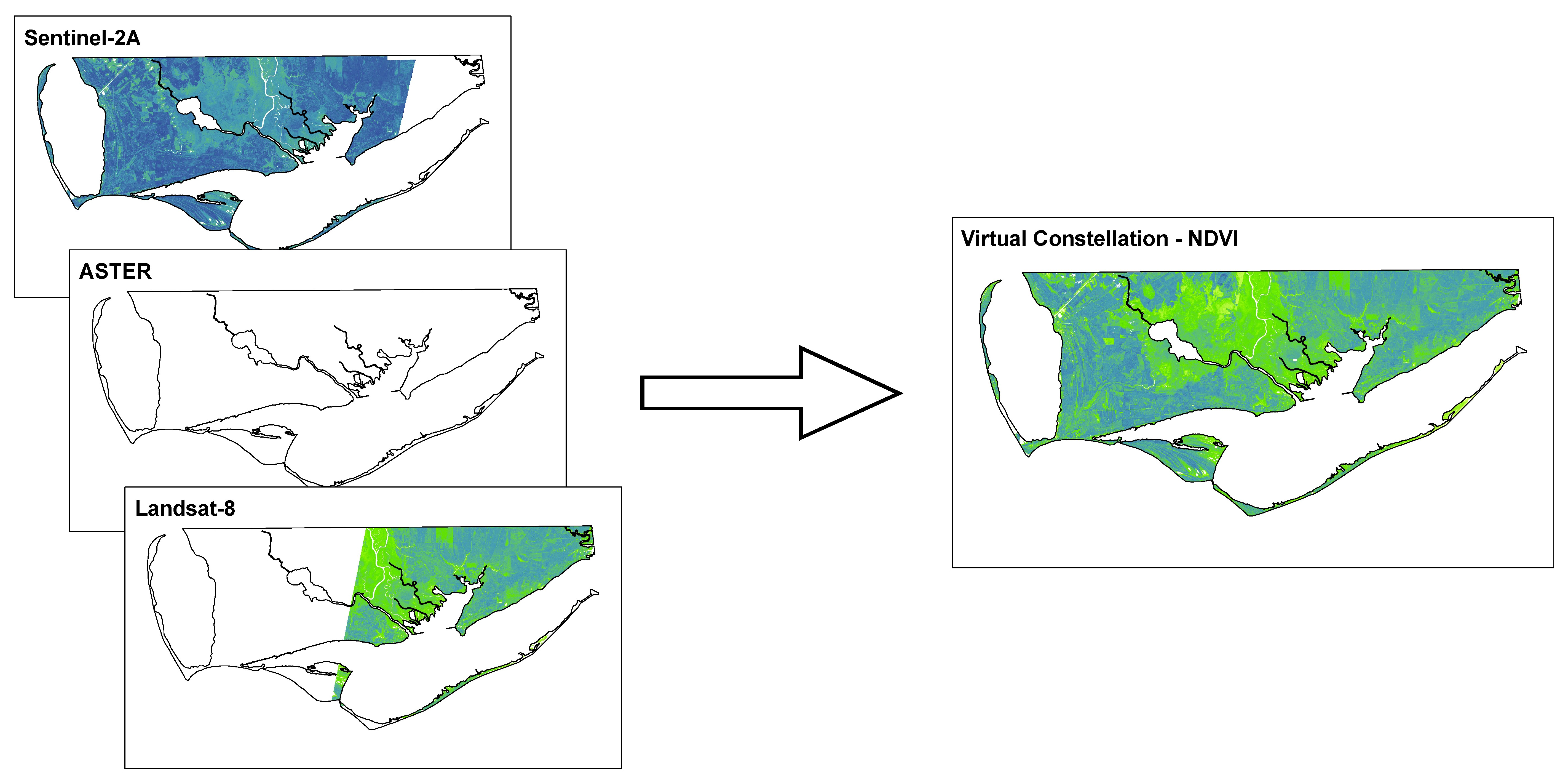
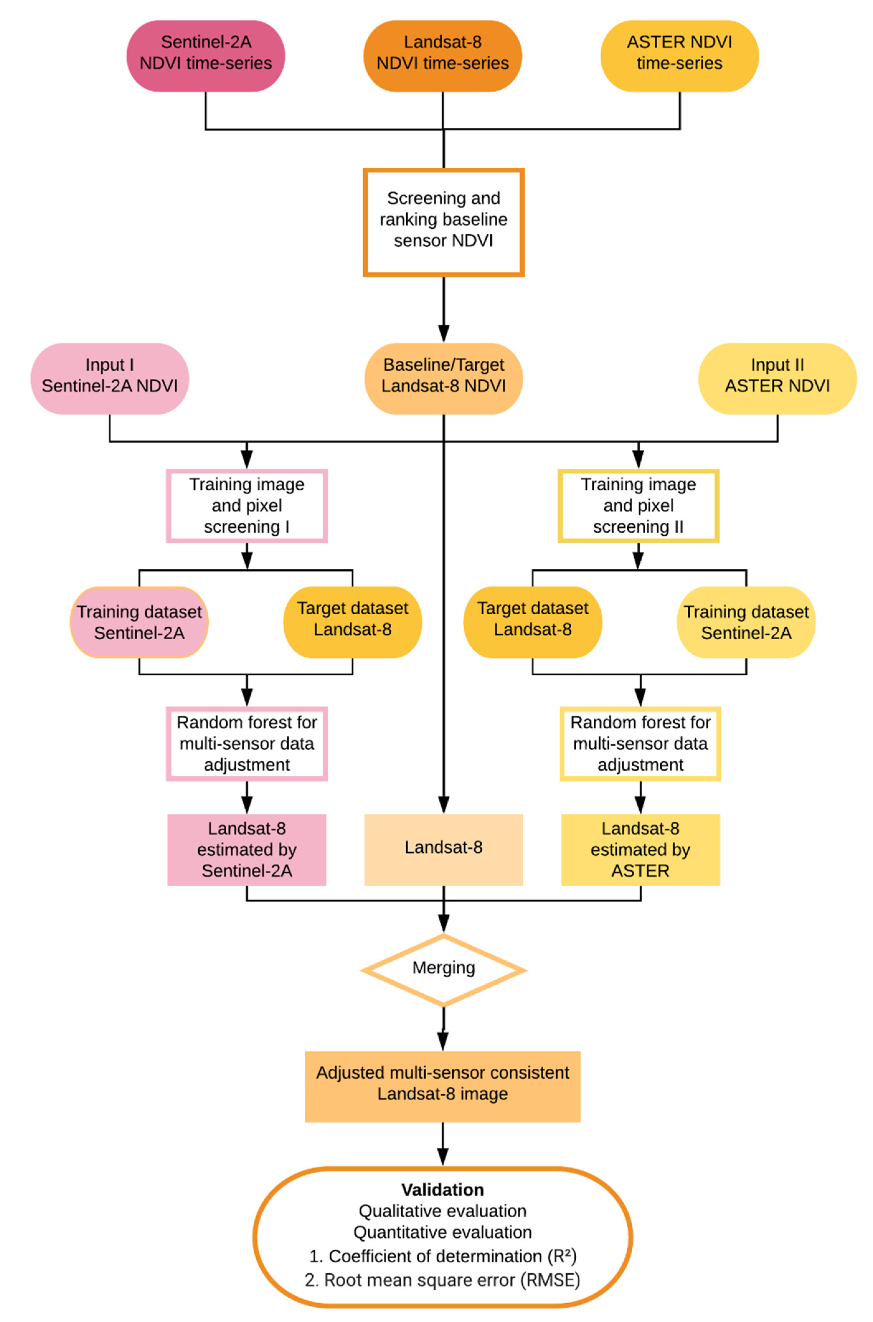
2.3. Virtual Constellation Development

The proposed virtual constellation is a remote sensing modeling system that integrates three satellite sensors to produce a single NDVI image each month that is free from cloud contamination (Figure 4). The method was developed under two assumptions regarding its primary application, long-term analysis of coastal marsh vegetation. First, we assume that NDVI is a proxy for overall CW vegetation health [54], and a monthly NDVI time series will follow a typical seasonal pattern except when influenced by major external forces such as sea level rise (long-term) or hurricane storm surge (short term). Second, inequality of NDVI between different sensors has systematic [20] and random [67] components and their relationship can be modeled using long-term historical data [68].
The first objective of the virtual constellation development was to align the NDVI value scales across the three sensors. Common observations from the three sensors during the coincident time-period (i.e., same calendar month) provided the opportunity for inter-sensor comparison. Relationships were analyzed at the pixel level between sensor pairs. The reason for developing the relationships between two sensors at a time is that each pair of sensors has unique inconsistencies from systematic and random error components [67]. The systematic inconsistency comes from climate conditions or geographical locations of the satellites [69] and the random inconsistency comes from multiple sources such as difference in overpass timing, sun angle, sensor mechanism and other sensor specific features. The amount of inconsistency varies in each sensor combination. Traditional (LR) would be the simplest method to establish NDVI relationships between sensors. However, LR has previously been shown to be ineffective in capturing complex relationships when synthesizing remote sensing imagery so the proposed virtual constellation implements an RF similar to previous research [54]. By using four years of monthly NDVI data adjusted to be compatible with L8 with sufficient temporal coincidence among the sensors, the RF was developed to predict NDVI values for L8 pixels obscured by clouds and shadows.

Random Forest Model

To establish quantitative relationships between the baseline sensor (L8) and peer sensors (S2A and ASTER) NDVI, we constructed an RF as a multivariate non-parametric regression method [70,71], using the peer sensor’s NDVI values, unique common geographic location (Northing (m) and Easting (m)) and month of the year from NDVI time series as predictor variables and baseline sensor’s NDVI values as target variable.
The RF algorithm builds many (typically between 100 and 1000) regression trees based on random subsamples, with replacement, from the training data set. This process is known as bootstrap aggregation, or bagging, and is used to train the individual trees with the results of the ensemble produced by computing the mean prediction (for regression) or the majority vote (for classification) [71,72]. At each node in a tree, a subset of predictor variables is selected at random and the optimal binary split is computed using the training data subsample and a metric known as “purity.” During this procedure, all candidate splits are evaluated to determine which one maximizes the purity of the resulting branch. Residual sum of squares (RSS), shown in Equation (2) is used as the splitting criteria for regression trees.
RSS = l e f t ( y i y L ) 2 + r i g h t ( y i y R ) 2
where, l e f t ( y i y L ) 2 and r i g h t ( y i y R ) 2 refer to the left and right nodes of the binary split, respectively.
The classification and regression trees in an RF grow to their maximum purity although they are commonly constrained by a maximum depth parameter. A key element in an RF is that each individual tree is exposed to only a randomly selected subset of the training data and must produce a prediction based on this limited information. Thus, it takes many trees to assemble a functional RF which also makes it resistant to overfitting. The number of trees is usually determined by an optimization procedure designed to calculate the minimum number of trees (for computational speed and efficiency) to achieve a desired result. RF is appealing in this application because of its generally accurate predictions and its calculation of feature importance that can act as a means for evaluating the influence of each feature on the algorithm [72]. Furthermore, RF models provide the user with additional randomness and computational efficiency during the bagging process. Splits within standard decision trees are typically determined by choosing an optimal split from all predictor variables. In contrast, an RF randomly selects a subset of the predictor variables, the number of which can be set as a parameter by the user. Subsequently, the best possible split is determined and used for that node. Further details regarding RF can be found in [71]. We also suggest that readers look at the figures of [54] to see an illustration of an example ensemble containing three trees and also a detail of one tree from the ensemble.

2.4. Application and Testing of Virtual Constellation in Apalachicola Bay

2.4.1. Selecting the Baseline Sensor

The baseline sensor is designated as the target sensor while the peer sensors provide complementary observations to the target sensor in an effort to estimate missing data. In this study, we used NDVI derived from three satellite systems (L8, S2A, and ASTER) for data fusion. Overall, three primary factors were considered when selecting the baseline sensor: Longest available historical data record; maximum overlapping with peer sensors; and minimum percentage of monthly cloud obscured data.
Cloud cover percentage (i.e., CC) was calculated as the number of cloud obscured pixels indicated in the imagery metadata divided by the total number of pixels in each image. The percentage of visible pixels (100–CC) for each sensor from 2013 to 2018 is shown in Figure 5.
As shown in Figure 5, Landsat (including previous generations) has the longest record dating back to August 1972. ASTER has the next longest record beginning in July 2000 and S2A has the shortest record beginning in July 2015. Figure 5 also shows that the coincident time period for all three sensors begins in 2015, therefore the period of analysis presented herein is from 2015 to 2018 when all three sensors were simultaneously operational (42 months total). These three sensors have spectral and spatial similarity which minimizes pre-processing and aids in information persistence during the analysis, especially in the sensors chosen as peers rather than primary. Along with the longest period of record, L8 has the highest percentage (~80%, S2A and ASTER have ~71 and ~52%, respectively) of visible data over the coincident time period from July 2015 to 2018, therefore it was selected as the primary sensor. Since L8 is the primary sensor, observations from the peer sensors can be integrated into the target L8 image when necessary. In other words, the output of virtual constellation is an L8 image where missing values due to clouds are estimated using S2A or ASTER.

2.4.2. Input Preparation

Images in the L8 time series were clipped to study area boundary using ArcGIS, excluding the major bays, lakes, and river channels from the analysis. In developing and training the virtual constellation, data availability was determined at the pixel scale. At 30 m resolution, there are approximately 1.17 million pixels in the image. The L8 cloud mask [73] distributed with each image was used to identify cloud pixels and calculate cloud cover percentage. An additional filter for negative NDVI values was implemented since NDVI values approaching −1 generally correspond to open water or other non-vegetated areas [74]. Figure 6 shows the temporal distribution of usable data in the study area over the analysis period. L8 NDVI imagery is released as a 16-day composite, therefore some months will contain two images. Due to the fact that the month, encoded as an integer from 1 to 12, is a predictor variable in the RF, in the event that two separate images were available for a particular month we selected the one with a lower CC.
S2A and ASTER NDVI (floating point values from 0.0 to 1.0), location (floating point Northing and Easting coordinates of the pixels in meters referenced to UTM Zone 16N, WGS84), and the image acquisition month (encoded as an integer from 1 to 12) were the predictor variables for the virtual constellation model. Including the location as an input feature enables the RF to estimate a value correlated with that of nearby pixels as well as a historically plausible value [54].
The pre-processed S2A and ASTER images were clipped to study area and resampled using a nearest neighbor assignment method to 30 m ground resolution using ArcGIS to maintain the consistency of each pixel location throughout the time series. The SEN2COR cloud mask [75] was used for S2A cloud identification. The negative NDVI filter mentioned previously was also used for S2A to mask out pixels corresponding to open water. In the virtual constellation model organization, S2A data are selected as secondary. The primary reason for prioritizing S2A over ASTER was that S2A was previously shown to provide adequate continuity for current LANDSAT missions [76]. Secondly, the ASTER NIR bandwidth is wider than the other two sensors and the difference between it and L8 is larger than the difference between S2A and L8 (Table 1). The L8-S2A fused imagery was then ready for tertiary fusion with ASTER if necessary. The virtual constellation model was robust in the sense that in cases of scene unavailability or obscurity for any single sensors, the others could be fused into viable NDVI imagery. In cases where only one sensor was available in addition to L8 (target sensor), then the peer sensors NDVI values were adjusted to L8 compatible NDVI and the L8 values remained unchanged. On the other hand, if the baseline sensor L8 was not available, then S2A was fused with ASTER where both transformed to L8 compatible values using the RF and fused into a virtual L8 image. In the event that the only available imagery is a cloudy image from one sensor, then a technique such as Optical Cloud Pixel Recovery (OCPR) would be necessary to repair the image [54].

2.4.3. Selection of Training Data

Machine learning models, including the virtual constellation proposed here, require reliable and clean data for training. The accuracy of the final estimator is dependent on the quantity and quality of the training data. All predictor variables except calendar month are floating point values. Across 42 months with approximately 1.17 million records (pixels) per month, the overall data corpus contained just over 49 million records.
The RF used in the virtual constellation to produce L8 compatible data from S2A and ASTER was implemented in Python using scikit-learn [77]. The Geospatial Data Abstraction Library (GDAL) [78] was used to determine the spatial locations associated with the data. All records containing missing predictors (labeled as “zero” or “NaN”) were removed. 70% (~34.4 million) of the records in the data corpus were randomly selected without replacement to form the training data set with the remaining 30% (~14.7 million) set aside as the testing data set. Examples of labeled records used in the virtual constellation model are shown in Table 2.

2.4.4. Validation and Performance

The first validation layer for the virtual constellation compares its prediction accuracy to a simple LR model. The purpose of this comparison is to demonstrate the superiority of the RF and justify the added complexity. In order to quantitatively validate the model, synthetic clouds were generated over areas in an image that have true NDVI values thus providing labeled data for testing. The images chosen for the synthetic cloud validation were purposely excluded from the training data but were within the study area. The metrics used for validation were Root Mean Square Error (RMSE) and Coefficient of Determination (R2).
RMSE is defined as:
RMSE = 1 n i = 1 n ( X i X i ^ ) 2
where X i and X i ^ represent the observed and estimated NDVI values for pixel i, respectively, and n is the number of pixels in the sample [79].
Coefficient of Determination (R2) is a measure of performance when comparing estimated values to observed values, typically in a one-to-one plot. It is defined as:
R 2 = 1 S S E S S X X
S S E = ( X i X i ^ ) 2
S S X X = ( X i X i ¯ ) 2
where Xi is the observed NDVI, X i ¯ is the mean of the observed NDVI values, and X i ^ is the estimated NDVI. R2 measures the linear agreement between predictions and observations or the degree to which the predicted values capture the observed values over simply using the mean as the prediction. However, it is sensitive to outliers and should only be used when the data are normally distributed.
As summarized above, synthetic clouds were created over pixels that had true L8 NDVI values. First, we compared the RF and LR virtual constellation models over the synthetic cloud pixels. Sample data from each season (3 month intervals) were used for performance assessment and validation. We also tested the virtual constellation model for sensitivity to the month and cloud cover percentage of the target image. The purpose of this analysis was to deepen our understanding about the performance of the model with respect to seasonality, check for issues related to Simpson’s paradox [54], and investigate the model’s sensitivity to the initial percentage of image obscured by clouds. Synthetic clouds were created by obscuring increasing percentages of the images to investigate the influence, if any, of cloud coverage in the target image on the end result and determine the working limitations of the model in this respect.

3. Results

3.1. Sensor NDVI Value Agreement

To investigate the degree of sensor agreement when producing NDVI for the same pixel at the same time, we developed one-to-one scatterplots of observed L8 versus observed S2A and observed ASTER individually, along with their counterpart plots of observed L8 versus adjusted S2A and adjusted ASTER (Figure 7). The NDVI images used to generate Figure 7 were acquired in May 2018. Figure 7A,C shows scale inconsistencies between L8 and observed S2A and observed ASTER, respectively, demonstrated by the different data ranges for each sensor. Figure 7A,C also shows a positive yet significantly scattered relationship between observed L8 and observed S2A and observed ASTER. Figure 7B,D show improved (less scattered) relationships after S2A and ASTER have been adjusted by the RF to estimate L8. A lower NDVI saturation point, at around 0.1, is evident for both S2A and ASTER compared to 0.2 for L8. On the higher end, L8 and S2A appear to saturate at approximately 0.8 and ASTER at approximately 0.6. There was less data dispersion around the trendline through the adjusted data shown in Figure 7B,D for both S2A and ASTER (R2 = 0.81 and 0.77, respectively), when compared to the observed NDVI for S2A and ASTER (R2 = 0.52 and 0.56, respectively) shown in Figure 7A,C. Note that the R2 values shown in Figure 7 were calculated from the 1000 point sub-sample used to generate that plot, however the trends are consistent with the results from the entire data set stated previously.

3.2. Data Fusion and Reconstruction

After implementing the virtual constellation model, the spatial coverage of L8 NDVI over the study area showed improvement. In February 2018 (Figure 8), L8 had visible coverage of only 48.1% of the study area. The coverage percentages improved to 100% after fusion with S2A. ASTER did not contribute to this fusion due to complete cloud coverage in its February 2018 image. In September 2016, both S2A and ASTER contributed to the increased spatial coverage of fused L8 NDVI. Before implementing the virtual constellation model, L8 had a visible coverage of only 9.89%. The visible coverage percentage improved to 33.75% after fusion with S2A and then to 70.86% after fusion with ASTER. Recall that the sharp image boundaries in Figure 8 represent the absence of an adjacent scene for that month. Additionally, it is important to note that the S2A and ASTER imagery shown in Figure 8 are in their raw NDVI state, prior to the RF adjustment to be L8 compatible.

3.3. Analysis of Virtual Constellation Model Performance

A large portion of L8 NDVI data in coastal areas is often missing due to heavy cloud cover (see Figure 3). Therefore, to aid in long-term continuous monthly monitoring of CW vegetation dynamics, a virtual constellation model was developed and applied to improve NDVI coverage.
In order to justify the use of a machine learning approach, the virtual constellation model using a RF to synthesize the NDVI data from the three satellite sensors was compared with one based on a simple LR [54]. The test data were NDVI values for pixels randomly selected without replacement (n = 830,772 total). For clarity, Figure 9 only shows the virtual constellation NDVI versus observed L8 NDVI for the test data from four months representing the four seasons (March, June, September, December), however the R2 and RMSE are calculated on the entire test set. Figure 9 (left) shows the predictions of RF virtual constellation while Figure 9 (right) shows the predictions of the LR based virtual constellation. The RF has a more consistent linear trend across the plotted seasons and tighter agreement than LR. The RF has an R2 value of 0.88 and a positive linear trend while the virtual constellation-LR has a weaker R2 value of 0.26 and is more scattered around its linear trendline, with some visible disjoints between seasons. On the test sample, the RF has a RMSE of 0.0020 while LR has a RMSE of 0.1207. The R2 and RMSE values suggest that the RF not only outperformed LR, but was also able to accurately estimate the absolute magnitude of NDVI. The data shown in Figure 9 are also color coded by month to represent seasonal variations and to investigate the possibility of the model performing well as a whole while simultaneously performing poorly in any individual month (Simpson’s Paradox). The four months shown in Figure 9 represent the seasonality of vegetation growth in this region. The colors are well distributed in the RF scatter plot indicating that the virtual constellation model is performing well in all individual months in addition to the entire time period.

3.4. Sensitivity of Virtual Constellation Performance to Initial L8 Cloud Cover

The virtual constellation model was trained and tested using a data corpus where each record corresponds to a labeled (NDVI) pixel with the predictor features explained above. The source images were compiled from L8, S2A, and ASTER imagery from the 2015 to 2018 time period. Since each pixel is used as a training record, rather than a vector representing the entire image (common practice in deep convolutional neural networks, for example), the virtual constellation avoids overfitting to any particular prediction feature, including month. However, in order to determine the effective limit on initial cloud cover in the target L8 image that can be reconstructed using the virtual constellation, we tested the method’s sensitivity to percent cloud cover by artificially obscuring increasing percentages of pixels from the target L8 image and executing the virtual constellation process. Table 3 shows the performance of the virtual constellation under different percentages of synthetic data loss. January 2016 was selected for the sensitivity analysis because it had 100% visibility and was therefore a good candidate for validation using synthetic data loss due to clouds.
Based on the analysis of the January 2016 image, the performance of the trained virtual constellation in reconstructing NDVI data in an L8 image was resilient to the initial cloud cover of the base L8 image. The R2 and RMSE values for predictions across the entire range of artificial cloud cover percentages were all greater than 0.81 and 0.0094. Thus, the results indicate that virtual constellation performs almost equally well regardless of season (Figure 9) or severity of cloud coverage in the target L8 image (Table 3).

4. Discussion

Sensor fusion can provide opportunities for capturing long-term monthly CW vegetation dynamics by creating spatially and temporally near-seamless observation records. The major hindrance to multi-sensor fusion is inconsistency between coincident images from each sensor and it is important to consider sensors that are compatible in terms of spectral and spatial characteristics. L8 and S2A have demonstrated potential for synergistic use that can capture the monthly dynamics of coastal areas. L8 and S2A data represent the most widely accessible moderate resolution multispectral satellite measurements. ASTER is another moderate resolution sensor that has similar spatial and spectral characteristics and was successfully used synergistically with previous generations of Landsat [80]. While multi-sensor NDVI data provide different views of earth surface, it is important to account for the sensor differences and ensure that the final products are aligned across all relevant dimensions prior to fusion. Otherwise, the uncorrected NDVI variances will introduce spurious noise into the fusion results [20].
The virtual constellation model presented here explicitly addresses this issue by adjusting each complementary sensor separately and fusing them hierarchically (S2A followed by ASTER). The current study provides a quantitative assessment of how the use of a virtual constellation, rather than relying on a single sensor, can advance the science of developing long-term, accurate, and seamless NDVI. It uses the properties of RF to model the relationship between a labeled outcome (NDVI) and the features used to predict it. Inclusion of coordinate location into the predictor set enables the model to estimate an appropriate value considering its neighboring pixels as well as a historically reasonable value for that location. Although, this renders the model specific to locations within the spatial reference system and units used here (UTM Zone 16 North, WGS 1984). Additionally, the inclusion of month only (encoded as an integer from 1 to 12) instead of both month and year enhances the model’s robustness to seasonality without overfitting to annual scale non-stationarity. Another reason for the selection of RF as the prediction interface between L8 and its supplemental sensors S2A and ASTER is its ability to estimate prediction error and feature importance simultaneously with model training and testing. This information can effectively guide researchers toward feature inclusion or exclusion as well as tuning the hyperparameters of the RF (number of features to split on and maximum depth). Table 4 shows the feature importance which is indicative of how useful each feature is in the construction of each RF decision trees used in virtual constellation for this study [81].
As shown in Table 4, the complementary sensor NDVI is the most important feature followed by position (Northing, Easting). The month contributes much less to the estimation, accounting for only 1.4 and 2.4% of the feature importance in the ASTER and S2A models, respectively. It is likely that the month adds a final layer of spatio-historical memory to the overall prediction, but perhaps it is replicating information already known to the model as a result of the complementary sensor NDVI. This is a potential topic for future work in enhancing virtual constellations.
The results also showed that using LR was insufficient to predict L8 NDVI for either complementary sensor. In terms of the wall clock time required to train the models, LR is significantly faster than RF. However, RF showed better prediction accuracy than LR in this application and its complexity is justified. The virtual constellation technique presented here was limited by the availability of historical data in which all three sensors were active. In particular, the peer sensor data (S2A and ASTER) are currently not available over the same long time period as the baseline Landsat 8 NDVI. Similar to many machine learning approaches, its performance is tightly coupled to the quality and quantity of its training data. It is not known, however, whether or not RF is the best machine learning model for this task. Based on the literature, it is a justifiable choice but perhaps as more data are collected, an alternative model such as convolutional neural networks may be a better choice. The authors also strongly recommend that the area of interest lie well inside the analysis boundary used to clip the satellite imagery to avoid interpolation effects near the edges. This is especially relevant to the technique presented here as the location was second only to peer sensor values in its influence on the final NDVI prediction.
The results presented herein also show that while the virtual constellation improves spatial coverage of obscured L8 NDVI imagery, there are still cases where it cannot reconstruct the image due to lack of complementary sensor data from S2A or ASTER over all or parts of the target image. One specific instance where this occurred was in October 2018. Figure 5 shows that no ASTER or S2A imagery was available for this month, and Figure 6 shows that only 45.75% of the L8 image was visible. Hurricane Michael made landfall on 10 October 2018 near the study region which likely caused the vast cloud cover rendering these images unusable. In these cases, a tool such as OCPR [54] that relies on deeper environmental data and no other sensors can be used. However, this also illustrates the potential for fusing images that occur in the same calendar month, but were acquired before and after a major event such as a hurricane. Future researchers should exercise caution and perhaps manually review imagery in months where catastrophic events affecting NDVI occurred.
There is also a possible issue when NDVI values from a complementary sensor are faulty and there are no accurate values in the other complementary or target sensors to prevent the faulty data from propagating into the output image. This issue is mitigated by quality control procedures implemented prior to the public release of the imagery. This is also mitigated to some degree by including the encoded location and month in the predictor feature set as NDVI values that are uncharacteristic for a specific location and time of year would likely be adjusted to more plausible values by the random forest.
Still, the virtual constellation model is a positive step towards producing spatially and temporally seamless NDVI for long-term CW studies. One crucial application where virtual constellation could be of use is the projection of CW coverage, zonation, and above ground biomass density under sea level rise scenarios [82,83,84,85]. A critical component of these studies is the ability to capture the present and past states of CW for validation purposes. Present and past states serve as the basis for future projections and these types of models are highly sensitive to initial conditions. A virtual constellation can be used to establish such initial states by capturing the spatial variability of CW vegetation health over time. It can also be used to validate a CW vegetation model’s projection as data are collected and produced in the future. However, additional work may be needed in the application of the negative NDVI filter used to exclude open water pixels in order to properly capture the permanent conversion of CW fringes to open water. At the monthly time scale, it is likely that all three sensors identify a similar set of open water pixels (since the negative NDVI filter is applied to each sensor’s image separately).

5. Conclusions

This study developed a machine learning technique for synergistic use of three optical satellite sensors to increase spatio-temporal coverage of NDVI imagery with cloud contaminated pixels in coastal wetlands. A virtual constellation using the random forest algorithm blended Landsat 8 OLI, Sentinel-2A MSI, and ASTER to produce enhanced NDVI imagery over the study area in Apalachicola, FL (USA) with improved spatial coverage. The enhanced NDVI imagery product was designed to correspond with the spatial and spectral properties of Landsat 8 NDVI. The salient benefit of using compatible sensor data is the retention of spatial patterns in the newly reconstructed NDVI imagery which is important for long-term evolution and change detection in monthly coastal wetland modeling.
While we see no major barriers to scaling this technique for operational use as all the included sensors develop to maturity and others are brought online, some future work including further tuning the random forest hyper parameters, accounting for catastrophic events that substantially alter the NDVI between complementary sensor acquisitions in the same calendar month, and addressing open water pixels in tidally influenced systems would be beneficial.
The idea of spatial information recovery using machine learning and multi-sensor fusion has been demonstrated to be a viable approach to mitigate cloud, shadow and other anomalous contamination with enough accuracy to support long-term coastal wetland studies. These applications would be strengthened by a deeper collaboration between the engineering and application communities. Stated another way, end-users would benefit from not only the new observation capabilities of proposed sensors, but also the redundancy and continuity they could provide to existing higher level data products.

Author Contributions

S.T.: Conceptualization, Methodology, Software, Formal Analysis, Data Curation, Writing—Original. S.C.M.: Validation, Writing—Review and Editing, Visualization, Supervision, Project Administration, Funding Acquisition. A.S.: Writing—Review and Editing, Supervision, Project Administration. All authors have read and agreed to the published version of the manuscript.

Funding

This research was funded in part under award NA16NOS4780208 from the National Oceanic and Atmospheric Administration (NOAA) Ecological Effects of Sea Level Rise (EESLR) Program. A.S. acknowledges the partial support from the Donors of the American Chemical Society.

Acknowledgments

S.C.M. would like to thank Joelle Bobinsky for her assistance in preparing Figure 2 and Figure 4. The authors are grateful for the efforts of the editorial staff and the anonymous peer reviewers for their consideration and constructive suggestions.

Conflicts of Interest

The authors declare no conflict of interest. The funders had no role in the design of the study; in the collection, analyses, or interpretation of data; in the writing of the manuscript, or in the decision to publish the results.

References

  1. Wulder, M.A.; Hilker, T.; White, J.C.; Coops, N.C.; Masek, J.G.; Pflugmacher, D.; Crevier, Y. Virtual constellations for global terrestrial monitoring. Remote Sens. Environ. 2015, 170, 62–76. [Google Scholar] [CrossRef] [Green Version]
  2. Dassenakis, M.; Paraskevopoulou, V.; Cartalis, C.; Adaktilou, N.; Katsiabani, K. Remote sensing in coastal water monitoring: Applications in the eastern Mediterranean Sea (IUPAC Technical Report). Pure Appl. Chem. 2011, 84, 335–375. [Google Scholar] [CrossRef]
  3. Xu, W.; Xie, A.; Huang, J.; Huang, B. A Method of Identifying Degradation of Ruoergai Wetland in Sichuan. In Proceedings of the IGARSS 2008—2008 IEEE International Geoscience and Remote Sensing Symposium, Boston, MA, USA, 7–11 July 2008; pp. 882–885. [Google Scholar]
  4. Barbier, E. Valuing Ecosystem Services for Coastal Wetland Protection and Restoration: Progress and Challenges. Resources 2013, 2, 213–230. [Google Scholar] [CrossRef] [Green Version]
  5. Barbier, E.B.; Hacker, S.D.; Kennedy, C.; Koch, E.W.; Stier, A.C.; Silliman, B.R. The value of estuarine and coastal ecosystem services. Ecol. Monogr. 2011, 81, 169–193. [Google Scholar] [CrossRef]
  6. Ozesmi, S.L.; Bauer, M.E.; Tiner, R.W.; Lang, M.W.; Klemas, V.V. Satellite remote sensing of wetlands. Wetl. Ecol. Manag. 2002, 10, 381–402. [Google Scholar] [CrossRef]
  7. Scheffler, D.; Frantz, D.; Segl, K. Spectral harmonization and red edge prediction of Landsat-8 to Sentinel-2 using land cover optimized multivariate regressors. Remote Sens. Environ. 2020, 241. [Google Scholar] [CrossRef]
  8. Gordon, H.R.; Wang, M. Retrieval of water-leaving radiance and aerosol optical thickness over the oceans with SeaWiFS: A preliminary algorithm. Appl. Opt. 1994, 33, 443–452. [Google Scholar] [CrossRef]
  9. Wald, L. Data fusion: A conceptual approach for an efficient exploitation of remote sensing images. In Proceedings of the 2nd International Conference “Fusion of Earth Data: Merging Point Measurements, Raster Maps and Remotely Sensed Images”, Sophia Antipolis, France, 28–30 January 1998; pp. 17–24. [Google Scholar]
  10. Campbell, A.D. Monitoring Salt Marsh Condition and Change with Satellite Remote Sensing. Ph.D. Thesis, University of Rhode Island, Kingston, RI, USA, 2018. [Google Scholar]
  11. Sun, C. Salt marsh mapping based on a short-time interval NDVI time-series from HJ-1 CCD imagery. In Proceedings of the American Geophysical Union Fall Meeting, San Francisco, CA, USA, 14–18 December 2015. [Google Scholar]
  12. Mo, Y.; Kearney, M.; Momen, B. Drought-associated phenological changes of coastal marshes in Louisiana. Ecosphere 2017, 8, e01811. [Google Scholar] [CrossRef]
  13. Tahsin, S.; Medeiros, S.C.; Singh, A. Resilience of coastal wetlands to extreme hydrologic events in Apalachicola Bay. Geophys. Res. Lett. 2016, 43, 7529–7537. [Google Scholar] [CrossRef]
  14. Civco, D.; Hurd, J.; Prisloe, S.; Gilmore, M. Characterization of coastal wetland systems using multiple remote sensing data types and analytical techniques. In Proceedings of the IEEE International Symposium on Geoscience and Remote Sensing, Denver, CO, USA, 31 July–4 August 2006; pp. 3442–3446. [Google Scholar]
  15. Zhukov, B.; Oertel, D.; Lanzl, F.; Reinhackel, G. Unmixing-based multisensor multiresolution image fusion. IEEE Trans. Geosci. Remote Sens. 1999, 37, 1212–1226. [Google Scholar] [CrossRef]
  16. Roy, D.P.; Ju, J.; Lewis, P.; Schaaf, C.; Gao, F.; Hansen, M.; Lindquist, E. Multi-temporal MODIS-Landsat data fusion for relative radiometric normalization, gap filling, and prediction of Landsat data. Remote Sens. Environ. 2008, 112, 3112–3130. [Google Scholar] [CrossRef]
  17. Kulawardhana, R.W.; Thenkabail, P.S.; Vithanage, J.; Biradar, C.; Islam Md, A.; Gunasinghe, S.; Alankara, R. Evaluation of the Wetland Mapping Methods using Landsat ETM+ and SRTM Data. J. Spat. Hydrol. 2007, 7, 62–96. [Google Scholar] [CrossRef]
  18. Cihlar, J. Identification of contaminated pixels in AVHRR composite images for studies of land biosphere. Remote Sens. Environ. 1996, 56, 149–163. [Google Scholar] [CrossRef]
  19. Zhu, W.; Pan, Y.; He, H.; Wang, L.; Mou, M.; Liu, J. A changing-weight filter method for reconstructing a high-quality NDVI time series to preserve the integrity of vegetation phenology. IEEE Trans. Geosci. Remote Sens. 2012, 50, 1085–1094. [Google Scholar] [CrossRef]
  20. Fan, X.; Liu, Y. Multisensor Normalized Difference Vegetation Index Intercalibration: A Comprehensive Overview of the Causes of and Solutions for Multisensor Differences. IEEE Geosci. Remote Sens. Mag. 2018, 6, 23–45. [Google Scholar] [CrossRef]
  21. Goodin, D.; Henebry, G. The effect of rescaling on fine spatial resolution NDVI data: A test using multi-resolution aircraft sensor data. Int. J. Remote Sens. 2002, 23, 3865–3871. [Google Scholar] [CrossRef]
  22. Fensholt, R.; Sandholt, I.; Proud, S.R.; Stisen, S.; Rasmussen, M.O. Assessment of MODIS sun-sensor geometry variations effect on observed NDVI using MSG SEVIRI geostationary data. Int. J. Remote Sens. 2010, 31, 6163–6187. [Google Scholar] [CrossRef]
  23. Roderick, M.; Smith, R.; Cridland, S. The precision of the NDVI derived from AVHRR observations. Remote Sens. Environ. 1996, 56, 57–65. [Google Scholar] [CrossRef]
  24. Galvão, L.S.; Vitorello, Í.; Almeida Filho, R. Effects of band positioning and bandwidth on NDVI measurements of Tropical Savannas. Remote Sens. Environ. 1999, 67, 181–193. [Google Scholar] [CrossRef]
  25. Padró, J.-C.; Pons, X.; Aragonés, D.; Díaz-Delgado, R.; García, D.; Bustamante, J.; Pesquer, L.; Domingo-Marimon, C.; González-Guerrero, Ò.; Cristóbal, J.; et al. Radiometric Correction of Simultaneously Acquired Landsat-7/Landsat-8 and Sentinel-2A Imagery Using Pseudoinvariant Areas (PIA): Contributing to the Landsat Time Series Legacy. Remote Sens. 2017, 9, 1319. [Google Scholar] [CrossRef] [Green Version]
  26. Claverie, M.; Ju, J.; Masek, J.G.; Dungan, J.L.; Vermote, E.F.; Roger, J.-C.; Skakun, S.V.; Justice, C. The Harmonized Landsat and Sentinel-2 surface reflectance data set. Remote Sens. Environ. 2018, 219, 145–161. [Google Scholar] [CrossRef]
  27. Zhang, H.K.; Roy, D.P.; Yan, L.; Li, Z.; Huang, H.; Vermote, E.; Skakun, S.; Roger, J.-C. Characterization of Sentinel-2A and Landsat-8 top of atmosphere, surface, and nadir BRDF adjusted reflectance and NDVI differences. Remote Sens. Environ. 2018, 215, 482–494. [Google Scholar] [CrossRef]
  28. Jiang, Z.; Huete, A.R.; Chen, J.; Chen, Y.; Li, J.; Yan, G.; Zhang, X. Analysis of NDVI and scaled difference vegetation index retrievals of vegetation fraction. Remote Sens. Environ. 2006, 101, 366–378. [Google Scholar] [CrossRef]
  29. Shang, R.; Zhu, Z. Harmonizing Landsat 8 and Sentinel-2: A time-series-based reflectance adjustment approach. Remote Sens. Environ. 2019, 235. [Google Scholar] [CrossRef]
  30. Li, W.; Du, Z.; Ling, F.; Zhou, D.; Wang, H.; Gui, Y.; Sun, B.; Zhang, X. A comparison of land surface water mapping using the normalized difference water index from TM, ETM+ and ALI. Remote Sens. 2013, 5, 5530–5549. [Google Scholar] [CrossRef] [Green Version]
  31. Wu, G.; Liu, Y. Satellite-based detection of water surface variation in China’s largest freshwater lake in response to hydro-climatic drought. Int. J. Remote Sens. 2014, 35, 4544–4558. [Google Scholar] [CrossRef]
  32. Flood, N. Comparing Sentinel-2A and Landsat 7 and 8 using surface reflectance over Australia. Remote Sens. 2017, 9, 659. [Google Scholar] [CrossRef] [Green Version]
  33. Li, S.; Ganguly, S.; Dungan, J.L.; Wang, W.; Nemani, R.R. Sentinel-2 MSI Radiometric Characterization and Cross-Calibration with Landsat-8 OLI. Adv. Remote Sens. 2017, 6, 147. [Google Scholar] [CrossRef] [Green Version]
  34. Gorroño, J.; Banks, A.C.; Fox, N.P.; Underwood, C. Radiometric inter-sensor cross-calibration uncertainty using a traceable high accuracy reference hyperspectral imager. ISPRS J. Photogramm. Remote Sens. 2017, 130, 393–417. [Google Scholar] [CrossRef] [Green Version]
  35. Hazaymeh, K.; Hassan, Q.K. Fusion of MODIS and Landsat-8 surface temperature images: A new approach. PLoS ONE 2015, 10, e0117755. [Google Scholar] [CrossRef]
  36. Arekhi, M.; Goksel, C.; Balik Sanli, F.; Senel, G. Comparative Evaluation of the Spectral and Spatial Consistency of Sentinel-2 and Landsat-8 OLI Data for Igneada Longos Forest. ISPRS Int. J. Geo. Inf. 2019, 8, 56. [Google Scholar] [CrossRef] [Green Version]
  37. Walker, J.; De Beurs, K.; Wynne, R.; Gao, F. Evaluation of Landsat and MODIS data fusion products for analysis of dryland forest phenology. Remote Sens. Environ. 2012, 117, 381–393. [Google Scholar] [CrossRef]
  38. Nie, Z.; Chan, K.K.Y.; Xu, B. Preliminary Evaluation of the Consistency of Landsat 8 and Sentinel-2 Time Series Products in An Urban Area—An Example in Beijing, China. Remote Sens. 2019, 11, 2957. [Google Scholar] [CrossRef] [Green Version]
  39. Zhu, Z.; Wang, S.; Woodcock, C.E. Improvement and expansion of the Fmask algorithm: Cloud, cloud shadow, and snow detection for Landsats 4–7, 8, and Sentinel 2 images. Remote Sens. Environ. 2015, 159, 269–277. [Google Scholar] [CrossRef]
  40. Xu, H.Q.; Zhang, T.J. Cross comparison of ASTER and landsat ETM+ multispectral measurements for NDVI and SAVI vegetation indices. Spectrosc. Spectr. Anal. 2011, 31, 1902–1907. [Google Scholar] [CrossRef]
  41. Mandanici, E.; Bitelli, G. Preliminary comparison of sentinel-2 and landsat 8 imagery for a combined use. Remote Sens. 2016, 8, 1014. [Google Scholar] [CrossRef] [Green Version]
  42. Chastain, R.; Housman, I.; Goldstein, J.; Finco, M.; Tenneson, K. Empirical cross sensor comparison of Sentinel-2A and 2B MSI, Landsat-8 OLI, and Landsat-7 ETM+ top of atmosphere spectral characteristics over the conterminous United States. Remote Sens. Environ. 2019, 221, 274–285. [Google Scholar] [CrossRef]
  43. Pohl, C.; Van Genderen, J.L. Review article Multisensor image fusion in remote sensing: Concepts, methods and applications. Int. J. Remote Sens. 1998, 19, 823–854. [Google Scholar] [CrossRef] [Green Version]
  44. Zhang, J. Multi-source remote sensing data fusion: Status and trends. Int. J. Image Data Fusion 2010, 1, 5–24. [Google Scholar] [CrossRef] [Green Version]
  45. Zhu, X.; Chen, J.; Gao, F.; Chen, X.; Masek, J.G. An enhanced spatial and temporal adaptive reflectance fusion model for complex heterogeneous regions. Remote Sens. Environ. 2010, 114, 2610–2623. [Google Scholar] [CrossRef]
  46. Tu, T.-M.; Su, S.-C.; Shyu, H.-C.; Huang, P.S. A new look at IHS-like image fusion methods. Inf. Fusion 2001, 2, 177–186. [Google Scholar] [CrossRef]
  47. Shettigara, V.K. A generalized component substitution technique for spatial enhancement of multispectral images using a higher resolution data set. Photogramm. Eng. Remote Sens. 1992, 58, 561–567. [Google Scholar] [CrossRef]
  48. Nunez, J.; Otazu, X.; Fors, O.; Prades, A.; Pala, V.; Arbiol, R. Multiresolution-based image fusion with additive wavelet decomposition. IEEE Trans. Geosci. Remote Sens. 1999, 37, 1204–1211. [Google Scholar] [CrossRef] [Green Version]
  49. Chavez, P.S.; Stuart, C.S.; Jeffrey, A.A. Comparison of Three Different Methods to Merge Multiresolution and Multispectral Data: LANDSAT TM and SPOT Panchromatic. Photogramm. Eng. Remote Sens. 1991, 57, 295–303. [Google Scholar] [CrossRef]
  50. Wei, Q.; Bioucas-Dias, J.; Dobigeon, N.; Tourneret, J.Y. Hyperspectral and Multispectral Image Fusion Based on a Sparse Representation. IEEE Trans. Geosci. Remote Sens. 2015, 53, 3658–3668. [Google Scholar] [CrossRef] [Green Version]
  51. Wang, Q.; Shi, W.; Atkinson, P.M.; Zhao, Y. Downscaling MODIS images with area-to-point regression kriging. Remote Sens. Environ. 2015, 166, 191–204. [Google Scholar] [CrossRef]
  52. Liu, Y.; Chen, X.; Wang, Z.; Wang, Z.J.; Ward, R.K.; Wang, X. Deep learning for pixel-level image fusion: Recent advances and future prospects. Inf. Fusion 2018, 42, 158–173. [Google Scholar] [CrossRef]
  53. Seo, D.K.; Kim, Y.H.; Eo, Y.D.; Lee, M.H.; Park, W.Y. Fusion of SAR and Multispectral Images Using Random Forest Regression for Change Detection. ISPRS Int. J. Geo. Inf. 2018, 7, 401. [Google Scholar] [CrossRef] [Green Version]
  54. Tahsin, S.; Medeiros, S.C.; Hooshyar, M.; Singh, A. Optical cloud pixel recovery via machine learning. Remote Sens. 2017, 9, 527. [Google Scholar] [CrossRef] [Green Version]
  55. Martinuzzi, S.; Gould, W.A.; Ramos González, O.M. Creating Cloud-Free Landsat ETM+ Data Sets in Tropical Landscapes: Cloud and Cloud-Shadow Removal; General Technical Report IITF-GTR-32; United States Department of Agriculture, Forest Service, International Institute of Tropical Forestry: Washington, DC, USA, February 2007.
  56. Jarihani, A.A.; McVicar, T.R.; van Niel, T.G.; Emelyanova, I.V.; Callow, J.N.; Johansen, K. Blending landsat and MODIS data to generate multispectral indices: A comparison of “index-then-blend” and “Blend-Then-Index” approaches. Remote Sens. 2014, 6, 9213–9238. [Google Scholar] [CrossRef] [Green Version]
  57. Goyal, A.; Guruprasad, R.B. A novel blending algorithm for satellite-derived high resolution spatio-temporal normalized difference vegetation index. In Proceedings of the Remote Sensing for Agriculture, Ecosystems, and Hydrology XX, Berlin, Germany, 10 October 2018. [Google Scholar]
  58. NOAA. The Coastal Change Analysis Program (C-CAP) Regional Land Cover; NOAA Coastal Services Center: Charleston, SC, USA, 1995.
  59. Tahsin, S.; Medeiros, S.C.; Singh, A. Wetland Dynamics Inferred from Spectral Analyses of Hydro-Meteorological Signals and Landsat Derived Vegetation Indices. Remote Sens. 2020, 12, 12. [Google Scholar] [CrossRef] [Green Version]
  60. Batie, S.S.; Wilson, J.R. Economic Values Attributable to Virginia’s Coastal Wetlands as Inputs in Oyster Production. J. Agric. Appl. Econ. 1978, 10, 111–118. [Google Scholar] [CrossRef] [Green Version]
  61. Lenhardt, C. Delivering NASA Earth Observing System (EOS) Data with Digital Content Repository Technology. Available online: https://processing.eos.com (accessed on 14 January 2019).
  62. Rousel, J.; Haas, R.; Schell, J.; Deering, D. Monitoring vegetation systems in the great plains with ERTS. In Proceedings of the Third Earth Resources Technology Satellite—1 Symposium, NASA SP-351, Washington, DC, USA, 10–14 December 1973; pp. 309–317. [Google Scholar]
  63. Park, S.K.; Schowengerdt, R.A. Image reconstruction by parametric cubic convolution. Comput. Vis. Graph Image Process. 1983, 23, 258–272. [Google Scholar] [CrossRef]
  64. Yamaguchi, Y.; Kahle, A.B.; Tsu, H.; Kawakami, T.; Pniel, M. Overview of Advanced Spaceborne Thermal Emission and Reflection Radiometer (ASTER). IEEE Trans. Geosci. Remote Sens. 1998, 36, 1062–1071. [Google Scholar] [CrossRef] [Green Version]
  65. Lynnes, C. A Simple, Scalable, Script-Based Science Processor. In Earth Science Satellite Remote Sensing; Qu, J.J., Gao, W., Kafatos, M., Murphy, R.E., Salomonson, V.V., Eds.; Springer: Berlin, Germany, 2007. [Google Scholar] [CrossRef]
  66. Krehbiel, C. Working with ASTER L1T Visible and Near Infrared (VNIR) Data in R. Available online: https://lpdaac.usgs.gov/resources/e-learning/working-aster-l1t-visible-and-near-infrared-vnir-data-r/ (accessed on 1 August 2020).
  67. Aghakouchak, A.; Mehran, A.; Norouzi, H.; Behrangi, A. Systematic and random error components in satellite precipitation data sets. Geophys. Res. Lett. 2012, 39. [Google Scholar] [CrossRef] [Green Version]
  68. Nay, J.; Burchfield, E.; Gilligan, J. A machine-learning approach to forecasting remotely sensed vegetation health. Int. J. Remote Sens. 2018, 39, 1800–1816. [Google Scholar] [CrossRef]
  69. Tian, Y.; Peters-Lidard, C.D.; Eylander, J.B.; Joyce, R.J.; Huffman, G.J.; Adler, R.F.; Hsu, K.L.; Turk, F.J.; Garcia, M.; Zeng, J. Component analysis of errors in Satellite-based precipitation estimates. J. Geophys. Res. Atmos. 2009, 114, D24101. [Google Scholar] [CrossRef] [Green Version]
  70. Rodriguez-Galiano, V.; Dash, J.; Atkinson, P.M. Intercomparison of satellite sensor land surface phenology and ground phenology in Europe. Geophys. Res. Lett. 2015, 42, 2253–2260. [Google Scholar] [CrossRef] [Green Version]
  71. Breiman, L. Random Forests. Mach. Learn. 2001, 45, 5–32. [Google Scholar] [CrossRef] [Green Version]
  72. Palmer, D.S.; O’Boyle, N.M.; Glen, R.C.; Mitchell, J.B. Random forest models to predict aqueous solubility. J. Chem. Inf. Modeling 2007, 47, 150–158. [Google Scholar] [CrossRef]
  73. Foga, S.; Scaramuzza, P.L.; Guo, S.; Zhu, Z.; Dilley Jr, R.D.; Beckmann, T.; Schmidt, G.L.; Dwyer, J.L.; Hughes, M.J.; Laue, B. Cloud detection algorithm comparison and validation for operational Landsat data products. Remote Sens. Environ. 2017, 194, 379–390. [Google Scholar] [CrossRef] [Green Version]
  74. Weier, J.; Herring, D. Measuring Vegetation: NDVI & EVI. Available online: https://earthobservatory.nasa.gov/features/MeasuringVegetation (accessed on 4 April 2019).
  75. Mueller-Wilm, U.; Devignot, O.; Pessiot, L. S2 MPC Sen2Cor Configuration and User Manual. Available online: https://step.esa.int/thirdparties/sen2cor/2.3.0/%5BL2A-SUM%5D%20S2-PDGS-MPC-L2A-SUM%20%5B2.3.0%5D.pdf (accessed on 1 August 2020).
  76. Topaloǧlu, R.H.; Sertel, E.; Musaoǧlu, N. Assessment of classification accuracies of Sentinel-2 and Landsat-8 data for land cover/use mapping. Int. Arch. Photogramm. Remote Sens. Spat. Inf. Sci. 2016, 41. [Google Scholar] [CrossRef]
  77. Pedregosa, F.; Varoquaux, G. Scikit-learn: Machine learning in Python. J. Mach. Learn. Res. 2011, 12, 2825–2830. [Google Scholar]
  78. GDAL/OGR Contributors. GDAL/OGR Geospatial Data Abstraction Software Library. 2020. Open Source Geospatial Foundation. Available online: https://gdal.org (accessed on 1 August 2020).
  79. Jagalingam, P.; Hegde, A.V. A Review of Quality Metrics for Fused Image. Aquat. Procedia 2015, 4, 133–142. [Google Scholar] [CrossRef]
  80. Nouha, M.; Saadi, A.; Mohamed Rached, B. Unmixing based Landsat ETM+ and ASTER image fusion for hybrid multispectral image analysis. In Proceedings of the 2007 IEEE International Geoscience and Remote Sensing Symposium, Barcelona, Spain, 23–28 July 2007; pp. 3074–3077. [Google Scholar]
  81. Rogers, J.; Gunn, S. Identifying Feature Relevance Using a Random Forest; Springer: Berlin/Heidelberg, Germany, 2006; pp. 173–184. [Google Scholar]
  82. Alizad, K.; Hagen, S.C.; Morris, J.T.; Medeiros, S.C.; Bilskie, M.V.; Weishampel, J.F. Coastal wetland response to sea-level rise in a fluvial estuarine system. Earth’s Future 2016, 4, 483–497. [Google Scholar] [CrossRef]
  83. Alizad, K.; Hagen, S.C.; Morris, J.T.; Bacopoulos, P.; Bilskie, M.V.; Weishampel, J.F.; Medeiros, S.C. A coupled, two-dimensional hydrodynamic-marsh model with biological feedback. Ecol. Model. 2016, 327, 29–43. [Google Scholar] [CrossRef] [Green Version]
  84. Morris, J.T.; Sundareshwar, P.V.; Nietch, C.T.; Kjerfve, B.; Cahoon, D.R. Responses of coastal wetlands to rising sea level. Ecology 2002, 83, 2869–2877. [Google Scholar] [CrossRef]
  85. Swanson, K.M.; Drexler, J.Z.; Schoellhamer, D.H.; Thorne, K.M.; Casazza, M.L.; Overton, C.T.; Callaway, J.C.; Takekawa, J.Y. Wetland Accretion Rate Model of Ecosystem Resilience (WARMER) and Its Application to Habitat Sustainability for Endangered Species in the San Francisco Estuary. Estuaries Coasts 2014, 37, 476–492. [Google Scholar] [CrossRef]
Figure 1. Location map of research setting in Apalachicola Bay, FL.
Remotesensing 13 00438 g001
Figure 2. Image pre-processing workflow. Tn represents a given satellite image acquisition date.
Remotesensing 13 00438 g002
Figure 3. Issues disrupting long term continuous NDVI coverage. (AC) Sentinel-2A August 2015, overlapping cloudy scenes from the same month merged. (D) ASTER May 2018 and (E) Landsat 8 February 2018, no adjacent scenes present during those months.
Remotesensing 13 00438 g003
Figure 4. Schematic flowchart of the virtual constellation process.
Remotesensing 13 00438 g004
Figure 5. Monthly percentage of visible pixels in the satellite imagery. The gray bars in the background are provided for scale and indicate 100% visibility.
Remotesensing 13 00438 g005
Figure 6. Percentage of scene visibility in Landsat 8 during random forest training time period.
Remotesensing 13 00438 g006
Figure 7. Comparison of observed NDVI differences between sensors and subsequent adjustments for 1000 randomly selected pixels in May 2018. Subfigure (A) shows Observed S2A versus Observed L8, (B) Random Forest Adjusted S2A versus Observed L8, (C) Observed ASTER versus Observed L8, and (D) Random Forest Adjusted ASTER versus Observed L8.
Remotesensing 13 00438 g007
Figure 8. Virtual Constellation performance for February 2018 and September 2016. White pixels in the project area indicate information loss due to clouds, shadows, or scene missing in that month.
Remotesensing 13 00438 g008
Figure 9. Estimated (random forest and linear regression) vs. observed NDVI.
Remotesensing 13 00438 g009
Table 1. Parameters of bands for NDVI computation from Landsat 8, Sentinel-2A, and ASTER.
SensorSubsystemBandSpectral Range (µm)Signal to Noise Ratio (SNR)Spatial Resolution (m)Swath Width (km)
Landsat 8
OLI
NIR50.85–0.8720430185
Red40.63–0.68227
Sentinel-2A
MSI
NIR8A0.86–0.887220290
Red40.65–0.6814210
ASTERNIR3N0.78–0.862021560
Red20.63–0.69306
Table 2. Sample data for training virtual constellation model.
L8 NDVIMonthNorthing (m)Easting (m)S2A NDVIASTER NDVI
0.5312692,842.03,295,065.00.490.37
0.5012692,872.03,295,065.00.530.40
0.414668,722.03,298,545.00.420.26
0.344668,752.03,298,545.00.690.21
0.149653,625.03,299,865.00.150.20
0.129653,655.03,299,865.00.110.29
0.116704,565.03,306,645.00.180.24
0.136704,625.03,306,645.00.630.23
0.655660,435.03,306,135.00.710.69
0.645660,465.03,306,135.00.690.65
Table 3. Sensitivity of virtual constellation performance to cloud cover in base image for January 2016.
Synthetic Cloud CoverR2RMSEp-Value
10%0.81290.009648<0.05
20%0.81460.009669<0.05
30%0.81270.009490<0.05
40%0.83560.009557<0.05
50%0.82460.009474<0.05
60%0.81790.009457<0.05
70%0.81130.009548<0.05
80%0.84030.009457<0.05
90%0.81550.009546<0.05
100%0.81930.009581<0.05
Table 4. Feature importance for the trained random forests.
ASTER to L8 NDVIS2A NDVI to L8
FeaturesImportanceFeaturesImportance
ASTER NDVI0.586S2A NDVI0.479
Northing (m)0.222Northing (m)0.275
Easting (m)0.185Easting (m)0.227
Month0.014Month0.024
Publisher’s Note: MDPI stays neutral with regard to jurisdictional claims in published maps and institutional affiliations.

