Article

Stand Delineation of Pinus sylvestris L. Plantations Suffering Decline Processes Based on Biophysical Tree Crown Variables: A Necessary Tool for Adaptive Silviculture

by
Mª Ángeles Varo-Martínez
and
Rafael M. Navarro-Cerrillo
*
Department of Forestry Engineering, Silviculture Laboratory, Dendrochronology and Climate Change, DendrodatLab—ERSAF, Campus de Rabanales, University of Cordoba, Crta. IV, km. 396, E-14071 Córdoba, Spain
*
Author to whom correspondence should be addressed.
Remote Sens. 2021, 13(3), 436; https://doi.org/10.3390/rs13030436
Submission received: 1 December 2020 / Revised: 29 December 2020 / Accepted: 21 January 2021 / Published: 27 January 2021

Abstract

:
Many planted Pinus forests are severely affected by defoliation and mortality processes caused by pests and droughts. The mapping of forest tree crown variables (e.g., leaf area index and pigments) is particularly useful in stand delineation for the management of declining forests. This work explores the potential of integrating multispectral WorldView-2 (WV-2) and Airborne Laser Scanning (ALS) data for stand delineation based on selected tree crown variables in Pinus sylvestris plantations in southern Spain. Needle pigments (chlorophyll and carotenes) and leaf area index (LAI) were quantified. Eight vegetation indices and ALS-derived metrics were produced, and seven predictors were selected to estimate and map tree crown variables using a Random Forest method and Gini index. Chlorophylls a and b (Chla and Chlb) were significantly higher in the non-defoliated and moderately defoliated trees than in severely defoliated trees (F = 14.02, p < 0.001 for Chla; F = 13.09, p < 0.001 for Chlb). A similar response was observed for carotenoids (Car) (F = 14.13, p < 0.001). The LAI also showed significant differences among the defoliation levels (F = 26.5, p < 0.001). The model for the chlorophyll a pigment used two vegetation indices, Plant Senescence Reflectance Index (PSRI) and Carotenoid Reflectance Index (CRI); three WV-2 band metrics, and three ALS metrics. The model built to describe the tree Chlb content used similar variables. The defoliation classification model was established with a single vegetation index, Green Normalized Difference Vegetation Index (GNDVI); two metrics of the blue band, and two ALS metrics. The pigment contents models provided R2 values of 0.87 (Chla, RMSE = 12.98%), 0.74 (Chlb, RMSE = 10.39%), and 0.88 (Car, RMSE = 10.05%). The cross-validated confusion matrix achieved a high overall classification accuracy (84.05%) and Kappa index (0.76). Defoliation and Chla showed the validation values for segmentations and, therefore, in the generation of the stand delineation. A total of 104 stands were delineated, ranging from 6.96 to 54.62 ha (average stand area = 16.26 ha). The distribution map of the predicted severity values in the P. sylvestris plantations showed a mosaic of severity patterns at the stand and individual tree scales. Overall, the findings of this work underscore the potential of WV-2 and ALS data integration for the assessment of stand delineation based on tree health status. The derived cartography is a relevant tool for developing adaptive silvicultural practices to reduce Pinus sylvestris mortality in planted forests at risk due to climate change.

Graphical Abstract

1. Introduction

Forest defoliation and mortality resulting from biotic and abiotic tree damage have been identified among the most significant disturbance and deleterious processes threatening the existence of forests in south-western Europe [1], being exacerbated due to climate change [2]. Forest decline may be caused by a variety of factors, including both natural processes, such as pests and diseases [3], climate variability [4], and fires [5], and anthropogenic activities (e.g., lack of silvicultural practices) [6] that alter the dynamics and ecological processes in the remnant vegetation. In the western Mediterranean Basin, Pinus sp. plantations are one of the most important environmental issues regarding climate change [7]. Forest decline in these ecosystems, caused mainly by droughts and forest pests, has quickly spread in latest years in the southeastern Iberian Peninsula [8]. Studies have shown that large areas of pine plantations are affected by these processes in southern Andalusia (southern Spain, [9]). Hence, these are some of the ecosystems most vulnerable to climate change in the Mediterranean area.
Forest decline and mortality processes include accelerated defoliation dynamics and changes in forest biophysical properties (e.g., Leaf Area Index-LAI, [10]), as well as alteration of biochemical variables in leaves (e.g., pigments, [11]). Therefore, the understanding of decline processes requires detailed, quantitative, accurate, and repeatable techniques (including defoliation mapping and analysis of biochemical properties) as well as the determination of their spatial distribution at the stand scale [12]. Forest decline assessment is mainly based on defoliation, changes in leaf pigments content, leaf water status, and crown structural changes in damaged forests [13,14]. Broadband multispectral remote sensing has been used to monitor forest defoliation and leaf pigment properties replacing traditional field assessment techniques [15]. Previous research has reviewed the assessment of forest decline based on field measurements, remote sensing [16,17], and geographic information systems (GIS) [18]. More recently, a new generation of multispectral sensors, such as WorldView-2 (WV-2), Rapid Eye, and Sentinel, has been widely used to link field defoliation measurements and remote sensing data [17,19]. Spectral information and vegetation indexes have provided acceptable classifications of defoliation [16]; however, the inclusion of structural information (especially the crown cover) is important since it can improve forest health assessment and mapping [14]. Therefore, Airborne Laser Scanning (ALS) has also been used to assess tree defoliation state and distinguish between healthy and defoliated trees [20,21]. Thus, the integration of multispectral and ALS high-resolution data offers many advantages in the evaluation of forest defoliation stage in forest ecosystems.
Sensor data integration is one of the best alternatives to traditional methods of stand delineation [22]. Those traditional methods based on photointerpretation and field data, although they have been useful for years, are limited by costs and by the impossibility of incorporating complex variables such as the vertical and horizontal structure of the canopy or the physiological state of the trees. Automatic processes based on image segmentation techniques improve complex relationships among silvicultural patterns and stand delineation methods [23]. In this context, quantification of the spatial distribution of selected tree crown properties, as visual and pre-visual predictors of forest decline at the stand scale, helps to improve our understanding of the dynamics of those processes and our development of adaptive strategies [24]. The use of crown and stand delineation based on multispectral and ALS data, as well as machine learning algorithms, has proven useful in these integration processes [23,25]. Additionally, the Gini inequality index has been broadly used in forest science [26], particularly in defoliation studies [27].
Therefore, stand delineation maps are a necessary tool to describe the declining status of forests, thus simplifying forest management; however, there is a lack of stand delineation studies based on biochemical properties [23]. Our hypothesis was that stand delineation in large Pinus plantations can be improved by using field biophysical variables and integrating data from multispectral sensors (e.g., from the WV-2 sensor) and ALS [28,29]. Therefore, the objective of this study was to develop a methodology for stand delineation based on the integration of defoliation (e.g., LAI) and biochemical properties (e.g., chlorophyll and carotenoids) using WV-2 and ALS data and a machine-learning modeling approach, based on tree crown delineation in Pinus sylvestris L. plantations. The methodology comprised three steps: (i) Accurate detection and delineation of individual trees using airborne LiDAR data, (ii) Determination of LAI, pigment content, and defoliation level at tree scale from WV-2 multispectral and ALS data using Random Forest algorithm, and (iii) Production of detailed tree/stand damage maps using the Gini inequality index. The main novelty of this work is based on the use of field biophysical parameters that describe the physiological status of the trees, its modeling by machine learning algorithms (e.g., Random Forest), and the segmentation using the Gini index. The cartography of stands based on biochemical properties is a necessary tool to estimate defoliation level and tree mortality episodes related to droughts and biotic agents in Pinus plantations, and the spatial data produced are critical to implementing adaptive silvicultural practices.

2. Materials and Methods

2.1. Study Area

The study area was located at Sierra de los Filabres (Andalusia region, Almería, south-eastern Spain, 37°22′N, 2°50′W; around 45,000 ha, between 750 and 2168 m.a.s.l; Figure S1, Supplementary Material). The average temperature over the whole year is 13.1 °C, with annual precipitation ranging between 300 and 400 mm. The xerorthents regosols are the dominant soils and steep slopes (>35%) describes the local topography with loam and silty loam textures. The current vegetation shows a marked altitudinal gradient and is strongly influenced by reforestation programs carried out between 1955 and 1983. The vegetation consists of a 40 to 50-year-old pine plantation dominated by Scots pine (Pinus sylvestris L.), with a current density between 509 and 1405 trees ha−1. The basal area ranges from 18.33 to 40.85 m2 ha−1 (Table 1).
A flowchart outlining the different methodological steps is provided in Figure 1.

2.2. Field Data

In July 2015, nine plots were settled within the range of the airborne LiDAR strips (Figure S1, Supporting Information) in P. sylvestris plantations. The plots were randomly located, and all trees with DBH ≥ 10 cm were measured. The diameter at breast height (1.3 m above ground level –DBH—cm) and height (H, m) were measured in circular plots with a radius of 12.6 m (500 m2) using Field-Map equipment (http://www.fieldmap.cz/) (Table 1). The crown defoliation was estimated for 430 trees by expert visual assessment based on the percentage crown decline and transparency according to the ICP-Forests protocol [30] (http://icp-forests.net/page/icp-forests-manual) (Figure S2, Supplementary Material). Defoliation was classified in percentage classes in 5% intervals (between 0 and 100) in comparison to a local “reference tree” [31]. The selected trees were in an area affected by drought-related mortality processes without the presence of pests and diseases [32]. Individual tree position was recorded using a sub-meter global satellite receiver (Leica Zeno 20 GIS, Leica Geosystems, Switzerland).
Three needle samples were taken from five trees in each plot (N = 135 samples, N = 45 trees) from branches with southern exposure, at the top of the tree crown, at noon (between 12:00 and 14:00, wintertime, GTM + 1). The needles were immediately protected from light exposure and frozen by placing them in foil envelopes that were then inserted in liquid nitrogen. Chlorophylls a and b (Chla and Chlb) and carotenoids (Car) were determined for a sample of 5 young needles (one-year-old) collected from the top of the crown. In the laboratory, the total leaf pigments were extracted and determined following the methodology of [33] (see [32,34] for further details). The pigments were expressed in content unit; that is, mass per unit leaf dry weight (mg g−1, Table 1).
Simultaneously, 45 LAI measures were taken with an LAI-2000 Plant Canopy Analyzer (PCA, LI-COR Inc., Lincoln, NE, USA) on the same trees selected for needle sampling (Table 1) as the average of five PCA readings per tree (height of about 1.3 m under clear sky conditions and less than 1 h before sunrise or after sunset [35]). The defoliation categories were analyzed statistically using one-way ANOVA, considering defoliation as the independent factor and biochemical variables (pigments and LAI) as the dependent variables. When difference among the defoliation levels was observed, the means were separated by Scheffe’s multiple range test for unequal sample sizes (p = 0.05) [36]. Statistical analyses were conducted using the R statistical package, version R-3.5.2 [37].

2.3. Remote Sensing Data

2.3.1. Airborne Laser Scanning Data

The ALS data were acquired on 10 April 2013 by the company Heliografics Fotogrametria S.L. (Alicante, Spain), using an ALS60 laser scanner (Leica-Geosystems AG, Heerbrugg, Switzerland) operated by plane from a flight altitude of 3300 m, and with an average point density of 10 points m−2 (Figure S1 Supplementary Material). The system operated at a scan frequency of 100 Hz and a laser pulse repetition rate of 158.2 kHz, and the FOV was 12 degrees, resulting in an illuminated footprint diameter of 32 cm (Table S1 Supplementary Material). The data were geo-referenced in the European Terrestrial Reference System 1989 (ETRS89) coordinate system. The 2-year time interval between the acquisition of the ALS data and the field data collecting period was considered negligible due to forest-stand homogeneity and the low annual height and diameter growth in the study area (dbh average annual increment of 3.58 ± 0.43 mm year−1).

2.3.2. WorldView-2 Images

For this study, orthorectified 8-bands WV-2 satellite imagery was selected because it improves the spatial and spectral analysis and the cartography and allows the monitoring of large areas in great detail and with deeper vegetation analysis [38]. The date of the flight was 10 July 2015. The imagery over the study area contained 0% cloud cover. The multispectral and panchromatic bands were ordered, with 2 m and 0.5 m spatial resolution, respectively. The imagery was obtained from the company DigitalGlobe (Spain) at a processing level of 1B. The pixel size at the geometric resolution (or ground sampling distance, GSD) of this band was 1.84 m in the nadir.
Previous to data analysis, the WV-2 image was processed by performing an atmospheric correction, a pan-sharpening technique, and orthorectification. The image was corrected atmospherically using the coefficients of the rational information polynomial (RPCs) provided by the satellite data. As differences in coordinates X and Y data were observed between the ALS data and remote sensing image, even though WV-2 data are sensor-based rectified (OrthoReady Standard-2A), a more specific orthorectification was conducted. Therefore, the 0.5 m pan-sharpened multispectral image was orthorectified, using 50 points taken as ground control points (GCPs) on WV-2 by considering the Canopy Height Model (CHM) calculated from the ALS data as a reference image for guidance and with assistance from an orthoimage (recorded in summer 2016, 0.5 m pixel size). Corrections achieved a RMSE of 0.72 pixels on the 0.5 m WV-2 imagery. The software ENVI 5.3 (Exelis Visual Information Solutions, Boulder, CO, USA) was used in all the processes made to the image and the FLASH tool was used for the atmospheric corrections.

2.4. Methods

2.4.1. Segmentation for Tree Crown Delineation

A segmentation based on ALS data was performed to detect and delineate individual trees. The “Pit-free” method of Khosravipour et al. [39] was used to create the canopy height model (CHM) with the LAStools software [40]. Next, the resulting CHM was used for the individualization of trees, following the Region Growing methodology with SAGA software [41]. Segmentation was accomplished by obtaining seeds from the Imagery-Segmentation option. Next, the seeds were used with the Simple Region Growing function, to calculate the growth regions (segments per individual tree) in raster format, so it was necessary to vectorize in QGIS software [42]. After running the tree delineation algorithm, the accuracy was evaluated with the reference 430 trees in the 9 testing plots, the recall (r, Equation (1)), precision (p, Equation (2)), and F-score (F, Equation (3)) were calculated using the methodology in Li et al. [43]:
r = T P T P + F N
p = T P T P + F P
F = 2 × r × p r + p
where TP (true positive) corresponds to a tree correctly segmented, FN (false negative or omission error) to a tree not segmented but assigned to a nearby tree, and FP (false positive or commission error) if a tree does not exist but is segmented from the point cloud.

2.4.2. LAI and Pigments Data Modeling

Eight published spectral indices were calculated for the WV-2 image and were evaluated to determine the relationship between the pigments content and LAI (Table 2). These indices have been proven to be effective throughout the remote sensing defoliation assessment literature [44] and in forest health evaluation [45]. The maximum, minimum, and mean values for each WV-2 band in every tree crown were computed. Thus, in total, 32 metrics were extracted from the image bands and indices. Additionally, from the ALS data, calculations of 61 metrics were performed for each tree crown delineated: namely statistics for the characterization of the return heights distribution, maximum, minimum, mean, standard deviation, percentiles of the return heights, percentiles of the first return heights, percentiles of return heights from the upper half of the tree, percentiles of return heights of first returns from the upper half of the tree, bincentiles of heights, bincentiles of heights from the first returns, bincentiles of height from the upper half of the tree, bincentiles of heights of first returns from the upper half of the tree, coverage percentage, and percentage of unique returns, of first returns, of last returns, and of intermediate returns. Thus, overall, there were 93 predictors (Table S2, Supplementary Material). All the ALS metrics were computed with lidR package v2.0.0 [46,47].
For defoliation level assessment, a Random Forest (RF) classification [49] was accomplished, while for every physiological data (chlorophyll a, chlorophyll b, carotenoids, and LAI) a k-NN regression model with Random Forest distance calculation was computed. In total, 300 segmented trees, from the 430 in which defoliation was evaluated (70% of the sample), were assigned to build a model for the prediction of classification stage, which included WV-2 and ALS metrics and defoliation data, using the RF non-parametric method [49]. This method has been extensively used to classify different types of remotely sensed data [50], including defoliation [51]. As the defoliation data were grouped in categorical values [31], the RF classifier method (instead of the regression method) was automatically selected by the program [49].
For the LAI and biochemical variables, 30 segmented trees (2/3 of those used to obtain the physiological data) were used to build a k-NN regression model [52]. From the different neighbors’ distance calculation methods for the models (Euclidean distance, Raw Euclidean without normalization, Mahalanobis distance, Independent Component Analysis distance, Most Similar Neighbor distance, Most Similar Neighbor with variance weighting, Random Forest distance, Random distance, and Gower distance), Random Forest was selected because of its demonstrated suitability in the study area [53].
Before developing the regression and classification models, a variance inflation factor (VIF) study was accomplished to inspect multicollinearity and select the best explanatory variables, considering VIF ≥ 10 as the stepwise elimination threshold [54]. Secondly, the most important variables for the imputation modeling were selected, using the generalized root mean square distance (grmsd) as the variables were added to a k-NN imputation model. Variables that strengthened the imputation were kept in the model while the rest were deleted. For this, we used the varSelection function from the yaImpute [52] package in the R statistical software [37]. We estimated the accuracy of the k-NN regression models by two validation procedures: internal cross-validation, in which two-thirds of the samples (30 segmented trees) were used, and an external validation, with the remaining samples. The RMSE, bias, and R2 were calculated for each process.
To estimate the defoliation accuracy of the RF classification model, a 10-fold, 5-times repeated cross-validated confusion matrix was constructed, using the 300 training trees, as well as a confusion matrix for external evaluation, using the evaluation dataset, consisting of the rest of the samples [55].
The RF classification and the k-NN regression model were performed using the “randomForest” [56], the “yaImpute” [52], and the “caret” packages [37,57]. The optimum value for the number of classification trees (ntree) and the number of variables (mtry) were randomly selected at each split in the tree building process [57] considering ntree values ranging from 500 to 2500 and mtry values extending from 1 to 10. This package also allows the k values to be tested, to achieve the best k-NN regression model.
Once the individual values of chlorophyll and defoliation had been assigned to each individual tree by the model prediction, the health status of all trees was assessed by the combination of both variables [58]. Both defoliation and discoloration (estimated as total chlorophyll) at the crown level were estimated on a 0–3 severity scale (Table 3).

2.4.3. Stand Delineation

Previous to stand delineation, individual tree variables (i.e., defoliation, biochemical variables, and severity classes) were summarized according to the Gini coefficient index (GI), Lorenz coefficient of asymmetry (LAC), the mean, minimum, and maximum values, and the number of trees per pixel, to characterize the hierarchy of the trees within the canopy at the pixel scale. The mean was substituted by the mode when the categorical data of defoliation were used. Each pixel had a size equivalent to that of the field plot.
From among the summary variables of the forest health structure, the GI was used to characterize the inequality of the tree defoliation, LAI, and biochemical variables at the pixel scale. The GI has been applied to discriminate stand structure variables [26,59]. The equations used to compute the GI are available in Duduman [60]. The GI ranges from 0 (perfect equality, where all values are the same) to 1 (maximum theoretical inequality). The ineq package [61] was used to calculate the GI and LAC of each spectral index against the defoliation, LAI, and biochemical variables.
Once the defoliation, LAI, pigments, and severity variables had been summarized by pixel, these variables were used to identify, and group single stands based on the physiological characteristics. Mean shift segmentation, implemented within OrpheoToolBox software (OTB) [62] for QGIS [42], was applied (Figures S2–S5 Supplementary Material). The OTB segmentation approach is a non-parametric density estimator based on the Parzen window [63] and was applied as explained in Varo-Martinez et al. [23]. Three parameters were set: (1) the spatial radius, to determine the boundaries of the neighborhood, (2) the range radius, to delimit the width in the spectral space, and (3) the minimum size of the regions to keep after clustering. A spatial radius of 2 was determined based on the nearby grouped spatial distribution of damaged trees observed in the study area, while the range radius and minimum size of the regions were chosen to fulfill the whole range that each parameter admitted.

2.4.4. Stand Cartography

Finally, a forest management map at the stand scale, based on the severity classes (Table 3), was generated. The stand maps were obtained using the tree-scale assessment, by applying the best models based on the WV-2 and LiDAR data to discriminate the stand health variables [59] and silvicultural status.

3. Results

3.1. Tree Crown Biochemical Variables of Different Defoliation Levels

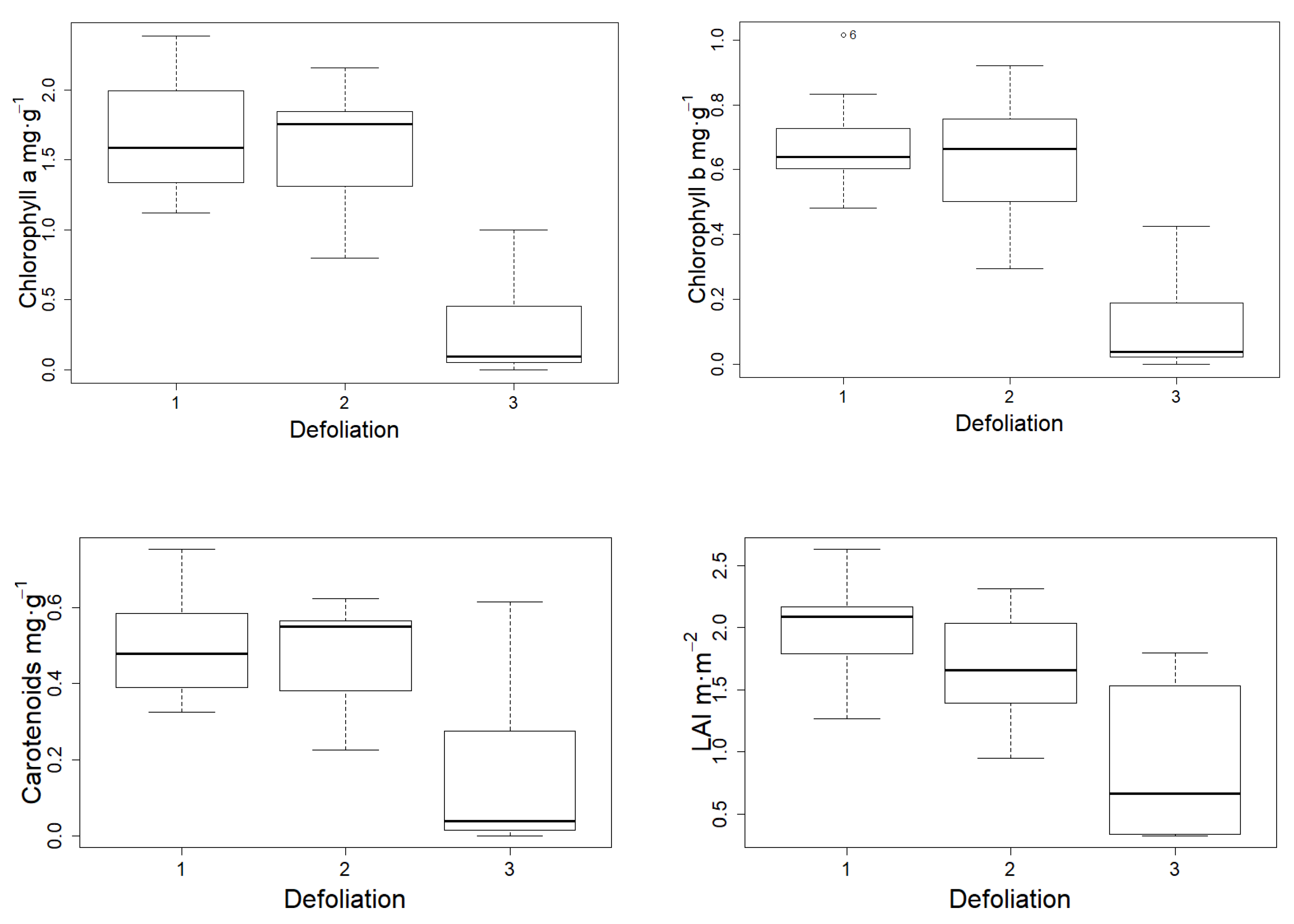
The means and the results of univariate ANOVA for the defoliation and biochemical variables are summarized in Figure 2. Chlorophylls a and b (Chla and Chlb) were significantly higher in the non-defoliated and slightly defoliated class (1.65 mg g−1 and 0.687 mg·g−1, respectively, and 2.34 mg·g−1 for the sum of Chla and Chlb) and in moderately defoliated trees (1.59 mg g−1 and 0.625 mg·g−1, respectively, and 2.21 mg·g−1 for the sum) than in severely defoliated trees (0.53 mg g−1 and 0.222 mg·g−1, respectively, and 0.75 mg·g−1 for the sum) (F = 14.02, p < 0.001 for Chla,; F = 13.09, p < 0.001 for Chlb; and F = 13.88, p < 0.001 for the sum of Chla and Chlb). A similar response was observed for carotenoids (Car), the values being significantly lower for the severely defoliated trees (0.159 mg g−1, F = 14.13, p < 0.001). The LAI also showed significant differences among the defoliation levels (F = 26.5, p < 0.001), with a response similar to that of the pigments (Figure 2). Therefore, it was possible to use the biophysical and biochemical variables (LAI and needle pigments) to separate the defoliation groups.

3.2. Individual Tree Crown Delineation Performance

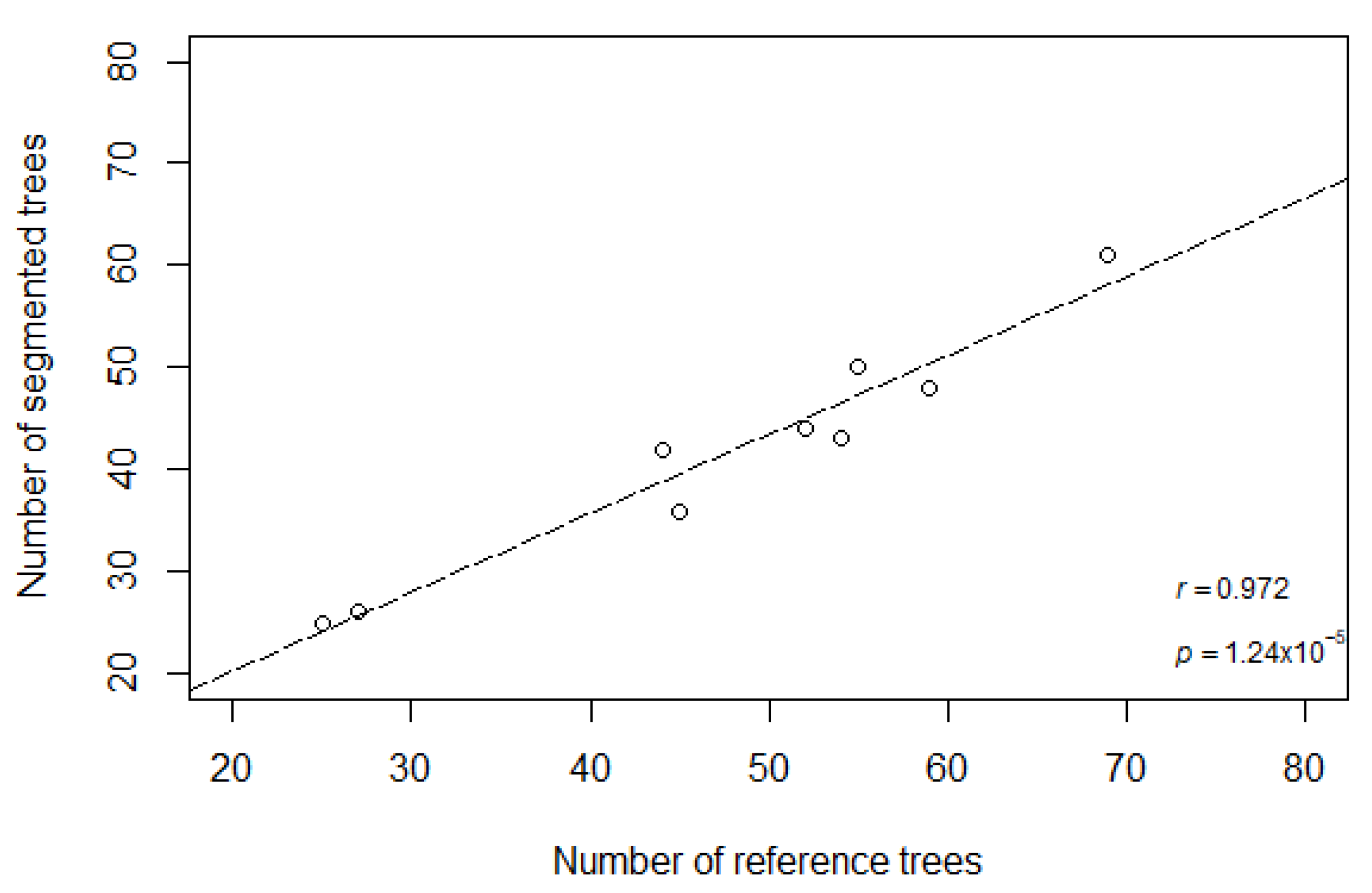
The accuracy assessment of tree delineation using the pit-free CHM generation method and the region growing segmentation are displayed in Table 4. Successful delineation exceeding 80% was achieved for all the plots. Figure 3 displays the R2 value (0.975, p < 0.01) for the fit of the linear regression model between the number of field and segmented trees for all plots, based on pit-free CHM and the region growing segmentation algorithm.

3.3. Models for Defoliation, LAI, and Needle Biochemical Parameter Estimations

From the 93 predictors, VIF separated 17 predictors within the variables from the ALS metrics and WV-2 bands and indices datasets for each biophysical and biochemical variable modeled. Each model used a different set of eight or fewer metrics, based on the grmsd as each one was added to the k-NN imputation model. The variable importance of the final models is described in Table 5 (Figure S3 Supplementary Material).
The model for the Chla used two vegetation indices, PSRI (Plant Senescence Reflectance Index) and CRI (Carotenoid Reflectance Index); three WV-2 band metrics, B4_max (maximum values in the delineated tree crown for band 4), B5_min (minimum values in the delineated tree crown for band 5), and B8_mean (mean values in the delineated tree crown for band 8); and three ALS metrics, zmin1r (minimum height of the first returns), binc60m (bincentil 60 for the upper half of the tree), and cov (percentage of first returns above 2 m). Interestingly, identical variables were also selected for the carotenoids regression model. The model built to describe the Chlb content used quite similar variables: the same vegetation indices and different image-based metrics applied to the same bands (the yellow, red, and second infrared). By contrast, binc60m was the only recurrent ALS metric.
With respect to LAI, no ALS metrics were selected. What the model required, instead, were WV-2 band metrics related to the green, yellow, and red visible electromagnetic spectrum region, B3_min (minimum values in the delineated tree crown for band 3), B4_min (minimum values in the delineated tree crown for band 4), B5_min (minimum values in the delineated tree crown for band 5), and B5_max (maximum values in the delineated tree crown for band 5), as well as the CRI vegetation index.
The defoliation classification model was established with a single vegetation index, GNDVI (Green Normalized Difference Vegetation Index); two metrics of the blue band, B2_mean (mean values in the delineated tree crown for band 2) and B2_max (maximum values in the delineated tree crown for band 2); and another two ALS metrics, binc40 (bincentil 40 in the delineated tree crown) and porclast (percentage of last returns in the delineated tree crown).
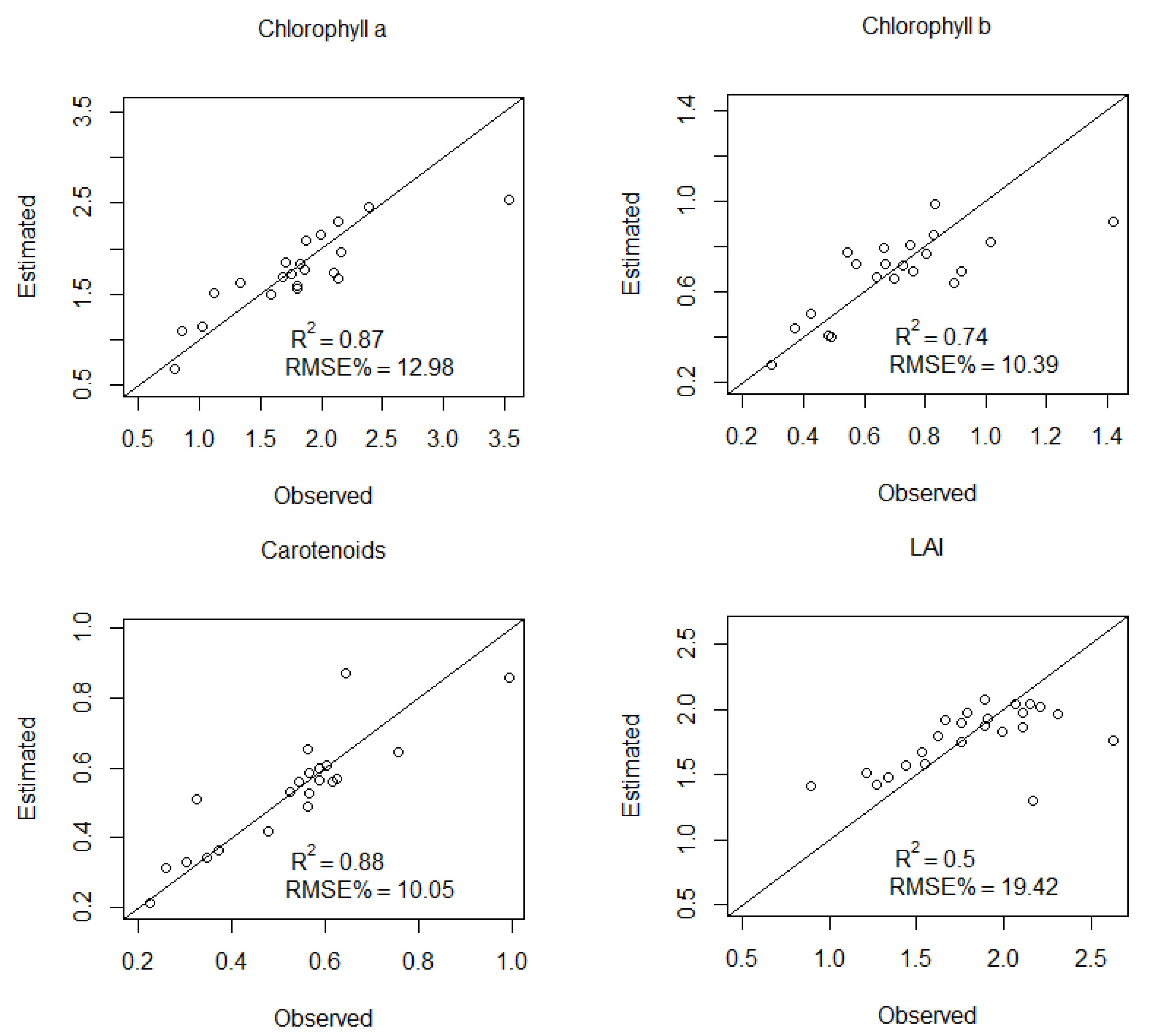
Scatter plots were computed for correlation analysis of the observed versus the estimated values for the LAI and pigments contents (Chla, Chlb, and Car), based on the RF algorithm in the k-NN modeling (Figure 4). The correlations obtained differed according to the leaf variable. The lowest coefficient of determination was obtained for LAI (R2 = 0.5, RMSE = 19.4%). The pigment contents models provided R2 values of 0.87 (Chla, RMSE = 12.98%), 0.74 (Chlb, RMSE = 10.39%) and 0.88 (Car, RMSE = 10.05%).
The cross-validated confusion matrix and the confusion matrix of the external evaluation outcoming from the RF classification for the defoliation model achieved a high overall classification accuracy (84.05% and 80.77%, respectively) and Kappa index (0.76 and 0.69, respectively) (Table 6) for the selected predictor dataset. Table 6 shows that the producer’s accuracies were very high for the three defoliation classes in the cross-validated confusion matrix (from 83.23% in healthy trees to 83.3% for defoliated individuals). The user’s accuracies were quite steady across the defoliation levels (from 85.42% for the healthy trees to 80% for the affected trees). In the confusion matrix with the evaluation data, the producer’s and user’s accuracy did not perform so evenly as in the cross-validated confusion matrix but still gave high values.

3.4. Stand Delineation and Stand Maps Based on Biophysical Variables

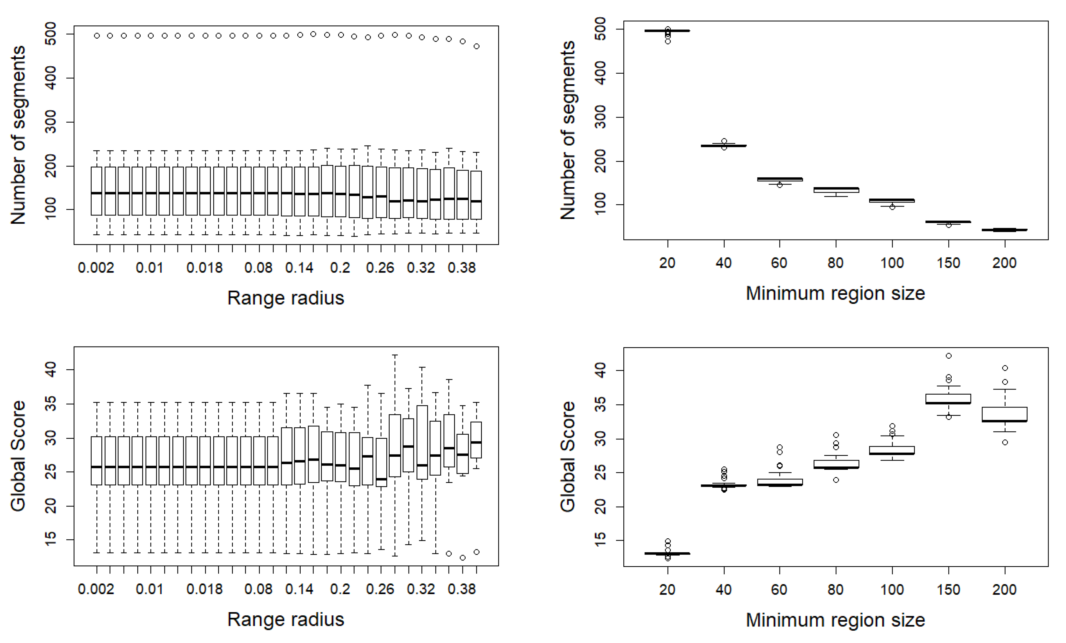
Figure 5 shows the behavior of the range radius and minimum region size parameters in the validation score of the segmentations and the number of resulting segments. It can be observed that as the minimum size of the region (measured in pixel units, which have the same area as the sample plots, 500 m2) increases, the number of segments drops, following an inverted exponential function. When a minimum region size of 20 is applied, the resulting segmentations have around 500 stands. On the other side of the curve, when a minimum region size of 200 is used, 50 stands are obtained.
However, the global score observed a positive correlation. The maximum global score was achieved with a minimum region size of 150. For higher values of this parameter, the segmentation results became worse. The range radius (expressed in normalized values between 0 and 1 for the whole set of layers that compounds the raster for segmentation) presented a flat response, both in the number of segments and in the global score, for the resulting segmentation.
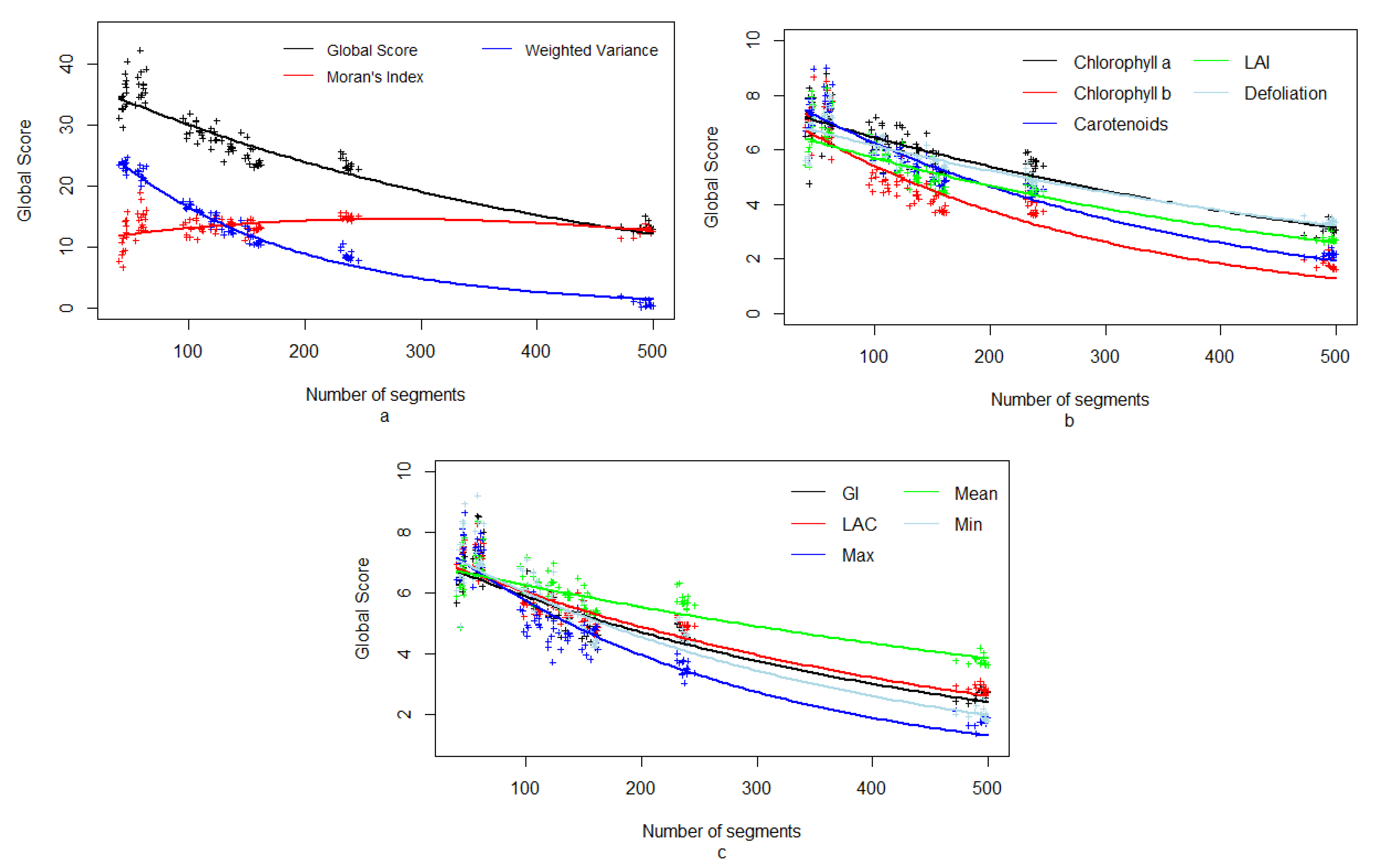
Figure 6 describes the performance of the set of segmentations in terms of the number of segments versus the score obtained. Figure 6b shows that defoliation and Chla were the layers with the best results in the validation of the segmentations and, therefore, in the generation of the stand delineation. Nevertheless, when the number of resulting segments was less than 100, the second most important variable was carotenoids. In Figure 6c, it is apparent that when the segments were large but few in number, the influence of the biophysical and biochemical variables (mean or mode, minimum, maximum, GI, and LAC value per pixel) was very similar. However, when the number of segments increased and the resulting stands were smaller, and the layer of mean values gained more relevance in the segmentation process, followed by GI and LAC.
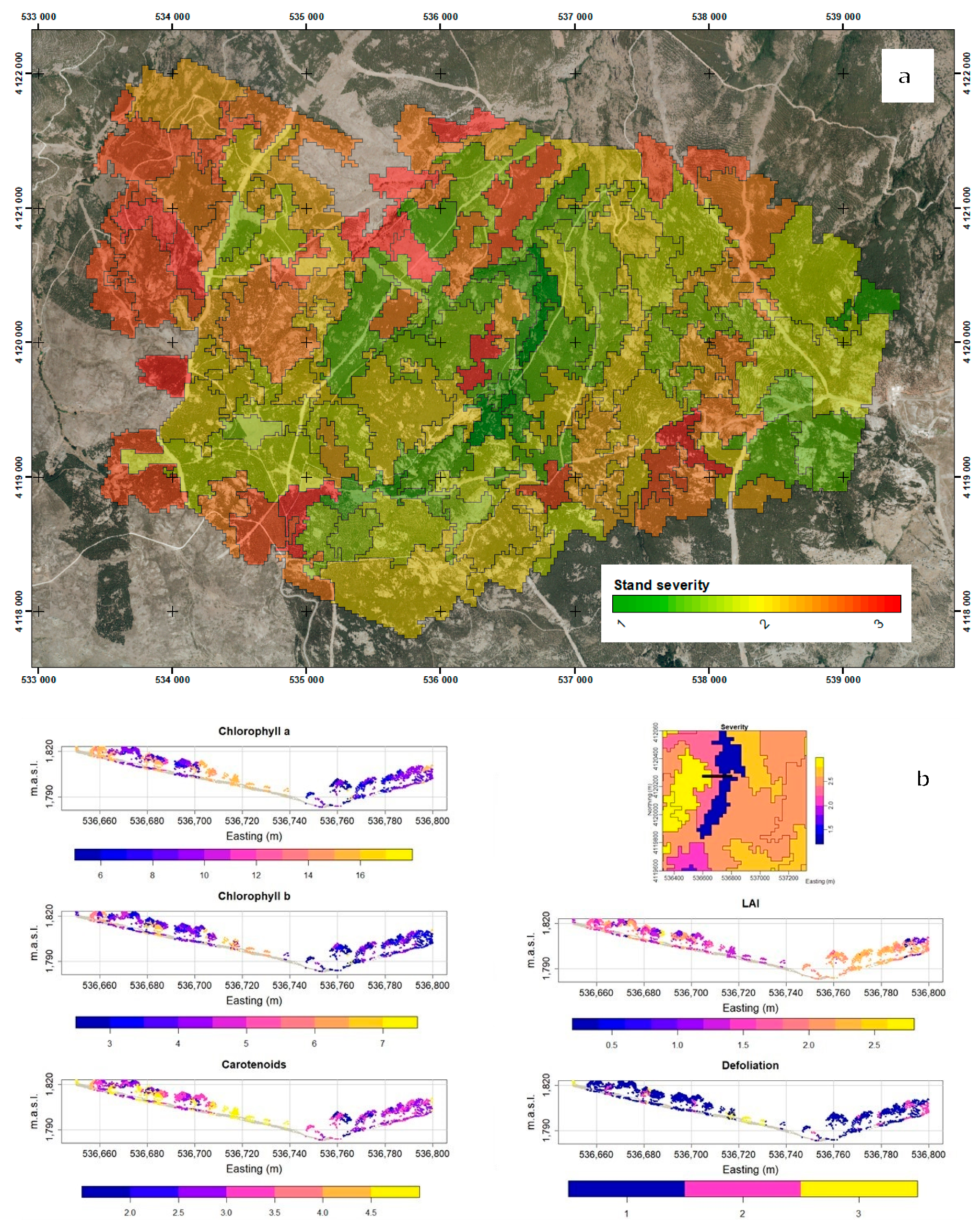
Figure 7 shows the best mapping results for the stand segmentation based on the individual tree defoliation, LAI, and pigments content (Chla, Chlb, Car, and defoliation). A total of 104 stands were delineated, ranging from 6.96 to 54.62 ha (average stand area = 16.26 ha) (Figure 7a). The distribution map of the predicted severity values in the P. sylvestris forested area showed a mosaic of severity patterns at the stand and individual scales (Figure 7a). The results confirm the high severity levels of the P. sylvestris plantations in the study area. In addition, some vertical sections of the stands were mapped using a combination of the tree crown condition and the ALS approach (Figure 7b), to show the individual tree crown condition.

4. Discussion

High-resolution canopy defoliation maps are a critical tool for assessing the impacts of forest decline dynamics, particularly under increasing forest decline related to drier and warmer climate scenarios [21,64]. This paper reports the feasibility of combining high-resolution multispectral WV-2 and ALS-derived structural signatures of Pinus plantations to detect and map tree health status and defoliation severity patterns in P. sylvestris plantations at the stand scale in southern Spain. We found that the combined use of WV-2 high-resolution multispectral images and ALS metrics is sensitive to stand delineation based on defoliation severity from the individual-tree to the stand levels. The present study also highlights the relevance of biophysical (LAI and defoliation) and biochemical (pigments contents) maps at the tree-stand scale in adaptive forest management, which has been considered less in prior studies (but see [23]). Therefore, this work is a new contribution to stand delineation in areas affected by forest decline processes, building on previous work [23,32].

4.1. Tree Crown Biochemical Variables at the Plot Level

One critical issue for defoliation assessment is the selection of biophysical and biochemical variables sensitive enough to detect the level of defoliation. Our results for the tree crown show that LAI and pigments (chlorophyll and carotenoids) were sensitive to variations in the tree defoliation severity. Forest decline causes significant disturbance because of substantial changes in leaf area [65]; thus, accurate LAI estimation is key in the assessment of forest health. LAI showed significant differences among the defoliation levels in the P. sylvestris plantations, with mean values ranging from 1.99 m·m−2, for healthy trees, to 0.64 m·m−2, in highly defoliated ones. In homogeneous canopies such as those of pine plantations, higher LAI values are expected for healthy vegetation. These results are consistent with other studies in P. sylvestris plantations under Mediterranean conditions [66]; although, a significant reduction in leaf area may be expected due to defoliation [20].
Earlier studies in the same location pointed out the influence of forest decline on the pigment content [32,34], showing its decrease in P. sylvestris in areas affected by drought-driven decline processes. In this study, the chlorophyll a and b (Chla and Chlb) contents were significantly higher in non-defoliated and moderately defoliated trees than in severely defoliated trees. Chla had a mean value of 1.65 mg g−1, with a maximum value of 2.38 mg·g−1 (healthy trees) and a minimum value of 0.53 mg g−1 (very damaged trees), while Chlb had an overall mean value of 0.69 mg g−1, with a maximum of 0.72 mg g−1 (healthy trees) and a minimum of 0.22 mg g−1 (very damaged trees). These values are consistent with previous values for this species (Chla, 1.4 to 2.4 mg g−1 and Chlb, 0.5 to 0.8 mg g−1, [67], but lower than in other studies [68]. A reduction in the chlorophyll content in conifers represents a typical photoprotection mechanism under stress conditions (e.g., drought, and high temperatures and radiation in our case [67,69].
A similar response was observed for carotenoids (Car): the values were significantly lower for the severely defoliated trees, ranging from a mean value of 0.49 mg g−1 for healthy individuals to a mean value of 0.16 mg g−1 for damaged trees. The Car content is more stable in stressed plants, to protect Chl and other components of the photosynthetic apparatus from photodestruction [70]. In contrast, Chlb is more sensitive to plant stress than Chla and Car [70].

4.2. Individual Tree Crown Delineation Performance

Individual tree detection has an important role when precise forest management is required. Successful tree identification is a key part of precision silviculture [43]. Several studies have shown that ALS data permit tree crown delineation in high-density forests [71], including pine plantations [72]. In this study, high-density ALS data (10 points m−2) were used for P. sylvestris tree crown delineation using a relatively simple segmentation algorithm. The pit-free canopy height model (CHM) segmentation method exhibited a strong performance in the delineation of P. sylvestris tree crowns (>80%). This result agrees with those obtained by Barnes et al. [73], which improved complete tree delineation accuracy for pit-free CHM inputs. Compared to natural forests, pine plantations host a low diversity of trees with respect to size and shape, which enables accurate tree delineation [74]. The use of high-density ALS data improved crown delineation, although low-density ALS data has also been successfully applied for individual tree crown delineation [14,43].

4.3. LAI and Pigments Modeling

Once individual tree crowns had been identified using the canopy segmentation process based on ALS data, segmented tree crowns were used to define homogeneous regions for the extraction of spectral and metric information. Most assessments of biophysical variables have used vegetation indices which are easy to use and show sufficient reliability [75]. Here, we selected relevant vegetation indices related to LAI, pigments, and defoliation, based on a literature search [76]. Based on the well-known relationship between these biophysical leaf parameters and green and red-edge bands, vegetation indices that include these bands have been extensively used in studies for damaged forest detection [76,77]. RF algorithm for k-NN distance calculation was applied to estimate P. sylvestris biophysical variables according to previous studies which have shown the ability of the RF method for the prediction of tree health status [78,79].
The LAI model included a set of metrics related to green, yellow, and red bands, as well as the CRI vegetation index, based on green and red-edge bands. Though the inclusion of green and yellow bands may seem unexpected, it is not unique [80]. As Fang et al. [81] stated, there is no universal relationship between LAI and any wavelength or vegetation index, as there are many influential factors such as vegetation type, sun-surface-sensor geometry, leaf chlorophyll content, background distance, and atmospheric quality. On the other hand, we found that visible and red-edge spectral indices, such as CRI, showed a high correlation with biophysical variables (i.e., LAI and defoliation) due to the better relationship with the physiological status of vegetation [75]. It can be inferred that the resulting model uses small color differences in tree crowns as well as the red-edge wavelength to predict LAI.
Regarding pigment models, CRI is an index that functions well in the prediction of the chlorophyll a, chlorophyll b, and carotenoids contents in tree crowns. Additionally, PSRI operates well for biochemical variables as it utilizes a combination of blue, red, and red-edge bands [82], which have been found to be sensitive to various stress factors at the leaf level [83]. PSRI has been proposed for the determination of the stage of leaf senescence because of its sensitivity to carotenoid accumulation [84]. Similar studies of chlorophyll at the leaf and canopy scales in pine forests have shown its relationship with visible and near-infrared single spectral indices [45,51]. Both vegetation indices specifically incorporate the red edge feature and have been recommended for chlorophyll prediction [77] as well as for their low sensitivity to the ground cover, biomass, and background [76]. These results are in concordance with previous studies showing the sensitivity of the red edge band to vegetation stress induced by insect pests [85]. However, concerning the role of WV-2 bands in pigment models, the yellow, red, and second infrared bands make relevant contributions.
Among the ALS metrics, we found binc60m to be a significant variable for three biochemical models. That may mean that trees with higher values of pigments have more returns around the middle parts of the crown, which might also be related to higher LAI values. Furthermore, for chlorophyll and carotenoids predictions, zmin1r and cov are decisive since they depend on the thickness of the canopy. Thus, our analysis shows that simple ALS metrics contributed to the model for pigments estimation (e.g., Chla and Car).
Finally, in the defoliation model, there can be seen an integration of GNDVI, a vegetation index combining the green band and the first infrared band together with metrics of the blue band and binc40 and porclast from the ALS metrics. These results are consistent with those of Meng et al. [21], who showed the sensitivity of the ALS metrics in the mapping of canopy defoliation. This can be explained by the fact that defoliation increases the “penetrability” of ALS pulses within the tree crown, leading to notable variations in the vertical profiles of the return points and providing a distinctive structural signature [14,86].
Previous studies have explored the use of ALS data to determine the defoliation of pine forests [20,87], but few have examined the integration of WV-2 vegetation indices and ALS metrics to measure biophysical and biochemical features at the individual tree level in Pinus plantations (however, see [14]). In this study, we explored the sensitivity of various ALS metrics with the intention of improving the mapping of LAI and pigments at the tree-crown scale. The integration of ALS metrics yielded good results for LAI and pigment estimation, suggesting accuracy and robustness in biophysical and biochemical parameter estimation [14,88]. Additionally, accurate selection of ALS metrics reduces the sensitivity to ground cover, biomass, and the backward scattering effect [89].
Limitations of the LAI and pigments models are related to the removal of all soil and under-crown vegetation effects from Pinus plantations and the overlaps of the spectral absorption characteristics of carotenoids and chlorophylls in the visible bands [90]. Using the tree segmentation procedure, some of the background effects (e.g., the distinction between the soil, grass, and tree spectra) were removed [91]. The use of crown delineation improved the generalized use of the defoliation severity model derived here. Additionally, differences in the forest understory on P. sylvestris plantations cannot explain differences in spectral changes due to the reduction in shrub cover [92]. However, the complete elimination of background signals from the tree spectra would ideally require signal unmixing [93]. Our results are consistent with many studies focused on the utility of remote sensing in the determination of the sensitivity of LAI and pigments to the defoliation [94]. They also show the potential of optimized vegetation indices in the assessment and mapping of vegetation defoliation and LAI. The integration of visible-NIR/IR/red-edge wavelengths and ALS metrics is a unique tool for improving the mapping of different defoliation/damage disturbances based on their structural fingerprint [95]. With the generalized availability in Europe of low-density ALS data, there is great potential for improving the monitoring of forest health [96].
The detection precision and kappa coefficient of the testing set suggest that RF has a strong modeling ability concerning the defoliation level assessment (overall accuracy 84.05%, κ = 0.76). This high accuracy could be related to the combined use of vegetation indices with an ALS segmentation. Misclassification mostly occurred between the low and medium defoliation levels, due to the overlapping of the lower range of defoliation in the latter with the higher range in the former. Despite this, the accuracies of the values were similar to or even better than those achieved in previous tree defoliation classifications. Navarro-Cerrillo et al. [14], using the same sensors, found an overall accuracy of 0.77, with a Kappa index of 0.69, for the discrimination between damage levels in savanna-like forests (e.g., dehesas).

4.4. Stand Delineation Based on Biophysical Variables

From the performance of the set of segmentations at different range radii and different minimum region sizes, shown in Figure 5, it can be inferred that variations in the range radius of the normalized biophysical and biochemical variables used in segmentation do not interfere with the ability to get the best results. This indicates that changes in the minimum, maximum, mean, GI, and LAC values of the variables between neighboring pixels are not large and so these values could be undergoing a gradual transition in the study area. Nevertheless, the variables can be segmented successfully when using relatively large areas for the minimum region size.
In view of the results in Figure 6a, due to the behavior of the algorithms, selection of the segmentation with the highest global score would give delineations with a very high internal variability (weighted variance) and little heterogeneity among stands (low Moran’s index). Moving to the opposite side of the curves, very internally homogeneous segments, very different from each other, were obtained, but at the cost of requiring a very high number of stands. Consequently, it is in the area where the curves intersect where better segmentation values were achieved because both the internal homogeneity and the external heterogeneity of the segments were compensated, making it easy to number and size the stands, from the forester’s point of view. A similar finding was reported in Varo-Martinez et al. [23].
Figure 6b leads us to conclude that when the stands were large, defoliation and Chla take on a more important role in the segmentation process; while, when the stands were smaller, Car became more important. This may be explained by the spatial distribution of Chla and Car in the study area. It can be inferred that the dispersion of Car in trees in neighboring pixels describes more appropriately what occurs on a small scale, whereas in extended areas the allocation of Chla in trees yields better-defined segmentations.
From Figure 6c, it can be inferred that the best summary parameters of the biophysical and biochemical variables are the mean or mode values per pixel together with Lorenz curves indices as indicators of the inequality inside the pixel. This means that the maximum and minimum values are rather constant in the study area. A stand map based on the defoliation and Chla values was finally produced for the P. sylvestris plantation (Figure 7).

4.5. Distribution Maps of Stands Based on Severity Classes

Severity-derived maps were obtained to describe the spatial patterns of forest decline, to support forest managers in developing adaptative silvicultural practices. Our results show that optimization of stand delineation based on biophysical and biochemical variables improves the accuracy of the representation of drought-induced defoliation. The inclusion of the leaf pigment content (e.g., Chla and Car) and defoliation in damage classification expresses the relationship between canopy physiological processes and pigment degradation and defoliation [97]. Highly damaged stands were more pervasive in the western and central parts of the study area. The same areas were previously identified as being more affected through the use of multispectral and hyperspectral sensors, areas with high percentage defoliation showing low pigment contents [32,34]. The predominance of defoliated stands in these areas could be because the western plantations were established on low-quality soils and with more restricted climatic conditions [14,98].

4.6. Adaptive Silvicultural Applications of Tree Health Workflow

Integrated LiDAR and multispectral maps provide more accurate spatial-temporal measurements of defoliation severity across multiple spatial scales, which are critical for designing adaptive forest management strategies to reduce forest damage [64,65,75,99]. The study area is located in the south-eastern part of Spain, in a region that has been severely affected by climate-driven defoliation and mortality of pine plantations since 2000 [32,98]. Application of the proposed P. sylvestris defoliation severity workflow based on WV-derived vegetation indices and simple ALS metrics provides a rapid and accurate approach to obtain spatially extensive tree damage maps at the individual tree level and segmented stand scale. As decline is driven not solely by defoliation but also by leaf pigment content changes (e.g., photodegradation of Chl and Car), the use of integrated maps (e.g., defoliation severity classes integrating LAI and pigments) was found to be more accurate compared to maps based only on defoliation. Moreover, if applied at the stand scale, these maps could show relevant information related to the spatial variation of tree health over large areas and could form the solid basis of a long-term forest health monitoring program.
Such stand maps may include other aspects besides tree health (silvicultural features, environmental variables, etc.) that are fundamental to forest management planning based on remote sensing data integration [14]. The development of spatially explicit maps might help to delineate sensitive areas regarding tree health, thereby helping forest managers to adapt silvicultural priorities to relieve or decrease the future impacts of decline damage in large and heterogeneous forest areas [21,63,73]. Additionally, the integration of visual and previsual approaches will be essential for anticipating the stress factor and the moment when a tree becomes visually unhealthy (see [100]).

5. Conclusions

In concordance with our previous studies, we have shown that the integration of WV-2 indices and ALS data-based metrics at the tree and stand scale resolutions provides a useful tool for the assessment of the tree and stand scale defoliation (LAI) and pigments (Chl and Car) over large spatial scales in defoliated P. sylvestris plantations. Given that this approach has a solid physical and biological basis, we recommend the use of ALS integrated into high-resolution multispectral data to derive forest severity maps in future work. After delineating each individual tree using ALS data, we successfully selected spectral indices and ALS-metric-based RF models to retrieve the defoliation severity and pigment contents. The enhanced performance of those indices achieved through the use of WV-2 data and ALS data confirm the option of using broad spectral regions to calculate chlorophyll indices. Additionally, the use of integrated severity categories (relying on defoliation and pigments concentrations) could increase the chance of early detection of tree stress. Finally, maps of individual tree defoliation severity at high spatial resolution (2 m) were obtained for the study area, based on ALS and WV-2 data. This allowed assessment of the spatial pattern of defoliation severity from the individual-tree level to the inter-stand level across severity gradients in Pinus plantations ecosystems at large spatial scales. Additionally, the integration of open access or low-price multispectral sensors (e.g., Landsat-8, HyspIRI, EnMap, GEDI, WorldView-3, Sentinel-2) with public ALS data can supply crucial information on canopy defoliation over large spatial-temporal scales, thus improving forest management alternatives to reduce forest damage (e.g., reduced growth and increased mortality). Research efforts should focus on early detection of tree stress in high-risk areas (forest under “climatic risk”), integrating detailed quantification of additional plant pigments (e.g., anthocyanins and carotenes), as well as hyperspectral and thermal and/or fluorescence data.

Supplementary Materials

The following are available online at https://www.mdpi.com/2072-4292/13/3/436/s1, Figure S1. Map of the study area in Sierra de los Filabres (Almería), showing the World View-2 scene, the LiDAR dataset, and the tree sampled field data. Figure S2. Examples of trees with different defoliation levels detected in the study area. A Level 1 Defoliation percentage <25% of foliage coverage. B Level 2 Defoliation percentage between 25% and 60% of foliage coverage. C Level 3 Defoliation percentage >60%. Figure S3. Scale variable importance of the variables used in selected models. Figure S4: Summarizing raster layers for Chlorophyll a concentration in every individual tree. Figure S5: Summarizing raster layers for Chlorophyll b concentration in every individual tree. Figure S6: Summarizing raster layers for Carotenoids concentration in every individual tree. Figure S7: Summarizing raster layers for LAI in every individual tree. Figure S8: Summarizing raster layers for defoliation levels in every individual tree. Table S1. Technical specifications of the ALS data. Table S2. Selected LiDAR and WorldView2 metrics parameters to run statistical analyses and modeling of Chlorophyll a, Chlorophyll b, Carotenoids, LAI, and defoliation.

Author Contributions

Conceptualization, R.M.N.-C. and M.A.V.-M.; Methodology, M.A.V.-M. and R.M.N.-C.; Formal Analysis, M.A.V.-M.; Investigation, R.M.N.-C. and M.A.V.-M.; Resources, R.M.N.-C.; Data Curation, M.A.V.-M.; Writing-Original Draft Preparation, R.M.N.-C. and M.A.V.-M.; Writing-Review & Editing, R.M.N.-C. and M.A.V.-M.; Project Administration, R.M.N.-C. All authors have read and agreed to the published version of the manuscript.

Funding

This research was funded by the Ministerio de Ciencia, Innovación y Universidades (Spain), through the ESPECTRAMED (CGL2017-86161-R) project and Junta de Andalucía through the ISOPINE (UCO-1265298).

Institutional Review Board Statement

Not applicable.

Informed Consent Statement

Not applicable.

Data Availability Statement

The data presented in this study are available on request from the corresponding author. The data are not publicly available due to institutional restrictions.

Acknowledgments

The authors thank the Ministerio de Ciencia, Innovación y Universidades (Spain), for providing the necessary financial support for this study through the ESPECTRAMED (CGL2017-86161-R), ISOPINE (UCO-1265298) and SilvAdapt RED2018 102719 T projects. We also acknowledge the institutional support of ESA (A)SAR data access (Project Number 54730) and the University of Cordoba-Campus de Excelencia CEIA3. We are grateful to David Walker for the English revision of the manuscript. Finally, the authors thank the colleagues of the Grupo de Evaluación y Restauración de Sistemas Agrícolas y Forestales-RNM-360, for their assistance in field work and other contributions to this study.

Conflicts of Interest

The authors declare no conflict of interest.

References

  1. Caudullo, G.; Barredo, J.I. A georeferenced dataset of drought and heat-induced tree mortality in Europe. One Ecosyst. 2019, 4. [Google Scholar] [CrossRef]
  2. Carnicer, J.; Coll, M.; Ninyerola, M.; Pons, X.; Sánchez, G.; Peñuelas, J. Widespread crown condition decline, food web disruption, and amplified tree mortality with increased climate change-type drought. Proc. Natl. Acad. Sci. USA 2011, 108, 1474–1478. [Google Scholar] [CrossRef] [Green Version]
  3. Trumbore, S.; Brando, P.; Hartmann, H. Forest health and global change. Science 2015, 349, 814–818. [Google Scholar] [CrossRef] [Green Version]
  4. Gustafson, E.J.; Sturtevant, B.R. Modeling forest mortality caused by drought stress: Implications for climate change. Ecosystems 2013, 16, 60–74. [Google Scholar] [CrossRef]
  5. Flannigan, M.D.; Amiro, B.D.; Logan, K.A.; Stocks, B.J.; Wotton, B.M. Forest fires and climate change in the 21st century. Mitig. Adapt. Strateg. Glob. Chang. 2006, 11, 847–859. [Google Scholar] [CrossRef]
  6. Nagel, T.A.; Firm, D.; Mihelic, T.; Hladnik, D.; Groot, M.; Rozenbergar, D. Evaluating the influence of integrative forest management on old-growth habitat structures in a temperate forest region. Biol. Conserv. 2017, 216, 101–107. [Google Scholar] [CrossRef]
  7. Gaztelurrutia, R.M.; Oviedo, J.A.B.; Pretzsch, H.; Löf, M.; Peinado, R.R. A review of thinning effects on Scots pine stands: From growth and yield to new challenges under global change. For. Syst. 2017, 26, 9. [Google Scholar]
  8. Camarero, J.J.; Linares, J.C.; Barreda, S.G.; Salguero, S.R.; Gazol, A.; Cerrillo, N.R.M.; Carreira, J. The multiple causes of forest decline in Spain: Drought, historical logging, competition and biotic stressors. In Dendroecology; Springer: Cham, Switzerland, 2017; pp. 307–323. [Google Scholar]
  9. Toro, T.J.; Cerrillo, N.R.M. Analysis of Site-dependent Pinus halepensis Mill. Defoliation Caused by ‘Candidatus Phytoplasma pini’ through Shape Selection in Landsat Time Series. Remote Sens. 2019, 11, 1868. [Google Scholar] [CrossRef] [Green Version]
  10. Bussotti, F.; Pollastrini, M. Observing climate change impacts on European forests: What work sand what does not in ongoing long-term monitoring networks. Front. Plant Sci. 2017, 8, 629. [Google Scholar] [CrossRef] [Green Version]
  11. Adams, H.D.; Zeppel, M.J.; Anderegg, W.R.; Hartmann, H.; Landhäusser, S.M.; Tissue, D.T.; Anderegg, L.D. A multi-species synthesis of physiological mechanism in drought-induced tree mortality. Nat. Ecol. Evol. 2017, 1, 1285–1291. [Google Scholar] [CrossRef]
  12. Laughlin, J.; Cook, P. Inventory-based forest health indicators: Implications for national forest management. J. For. 2003, 101, 11–17. [Google Scholar]
  13. Dobbertin, M.; Hug, C.; Mizoue, N. Using slides to test for changes in crown defoliation assessment methods. Part I: Visual assessment of slides. Environ. Monit. Assess. 2004, 98, 295–306. [Google Scholar] [CrossRef] [PubMed] [Green Version]
  14. Cerrillo, N.R.M.; Martínez, V.M.Á.; Acosta, C.; Rodriguez, G.P.; Cuesta, S.R.; Gomez, R.F. Integration of WorldView-2 and airborne laser scanning data to classify defoliation levels in Quercus ilex L. Dehesas affected by root rot mortality: Management implications. For. Ecol. Manag. 2019, 451. [Google Scholar] [CrossRef]
  15. Huang, C.Y.; Anderegg, W.R.; Asner, G.P. Remote sensing of forest die-off in the Anthropocene: From plant ecophysiology to canopy structure. Remote Sens. Environ. 2019, 231. [Google Scholar] [CrossRef]
  16. Wulder, M.A.; Dymond, C.C.; White, J.C.; Leckie, D.G.; Carroll, A.L. Surveying mountain pine beetle damage of forests: A review of remote sensing opportunities. For. Ecol. Manag. 2006, 221, 27–41. [Google Scholar] [CrossRef]
  17. Stone, C.; Mohammed, C. Application of remote sensing technologies for assessing planted forests damaged by insect pests and fungal pathogens: A review. Curr. For. Rep. 2017, 3, 75–92. [Google Scholar] [CrossRef]
  18. Lausch, A.; Erasmi, S.; King, D.; Magdon, P.; Heurich, M. Understanding forest health with remote sensing-part II—A review of approaches and data models. Remote Sens. 2017, 9, 129. [Google Scholar] [CrossRef] [Green Version]
  19. Sapkota, B.; Liang, L. A multistep approach to classify full canopy and leafles strees in bottom land hard woods using very high-resolution imagery. J. Sustain. Forest. 2018, 37, 339–356. [Google Scholar] [CrossRef]
  20. Solberg, S.; Næsset, E.; Hanssen, K.; Christiansen, E. Mapping defoliation during a severe insect attack on Scots pine using airborne laser scanning. Remote Sens. Environ. 2006, 102, 364–376. [Google Scholar] [CrossRef]
  21. Meng, R.; Dennison, P.; Zhao, F.; Shendryk, I.; Rickert, A.; Hanavan, R.; Cook, B.; Serbin, S. Mapping canopy defoliation by herbivorous insects at the individual tree level using bi-temporal airborne imaging spectroscopy and LiDAR measurements. Remote Sens. Environ. 2018, 215, 170–183. [Google Scholar] [CrossRef]
  22. Eysn, L.; Hollaus, M.; Schadauer, K.; Pfeifer, N. Forest delineation based on airborne LIDAR data. Remote Sens. 2012, 4, 762–783. [Google Scholar] [CrossRef] [Green Version]
  23. Martínez, V.M.Á.; Cerrillo, N.R.M.; Clemente, H.R.; Lazo, D.J. Semi-automated stand delineation in Mediterranean Pinus sylvestris plantations through segmentation of LiDAR data: The influence of pulse density. Int. J. Appl. Earth Obs. 2017, 56, 54–64. [Google Scholar] [CrossRef] [Green Version]
  24. Anderegg, W.; Hicke, J.; Fisher, R.; Allen, C.; Aukema, J.; Bentz, B.; Pan, Y. Tree mortality from drought, insects, and their interactions in a changing climate. New Phytol. 2015, 208, 674–683. [Google Scholar] [CrossRef] [PubMed]
  25. Belgiu, M.; Drăguţ, L. Random forest in remote sensing: A review of applications and future directions. ISPRS J. Photogramm. Remote Sens. 2016, 114, 24–31. [Google Scholar] [CrossRef]
  26. Valbuena, R.; Eerikäinen, K.; Packalen, P.; Maltamo, M. Gini coefficient predictions from airborne lidar remote sensing display the effect of management intensity on forest structure. Ecol. Indic. 2016, 60, 574–585. [Google Scholar] [CrossRef]
  27. Marx, A.; Kleinschmit, B. Sensitivity analysis of RapidEye spectral bands and derived vegetation indices for insect defoliation detection in purê Scots pine stands. iForest 2017, 10, 659–668. [Google Scholar] [CrossRef] [Green Version]
  28. Antonarakis, A.S.; Munger, J.W.; Moorcroft, P.R. Imaging spectroscopy-and lidar-derived estimates of canopy composition and structure to improve predictions of forest carbon fluxes and ecosystem dynamics. Geophys. Res. Lett. 2014, 41, 2535–2542. [Google Scholar] [CrossRef]
  29. Beland, M.; Parker, G.; Sparrow, B.; Harding, D.; Chasmer, L.; Phinn, S.; Strahler, A. On promoting the use of lidar systems in forest ecosystem research. For. Ecol. Manag. 2019, 450. [Google Scholar] [CrossRef]
  30. Eichhorn, J.; Roskams, P.; Ferretti, M.; Mues, V.; Szepesi, A.; Durrant, D. Visual Assessment of crown condition and damaging agents. Manual Part IV. In Manual on Methods and Criteria for Harmonized Sampling, Assessment, Monitoring and Analysis of the Effects of Air Pollution on Forests; UNECE ICP Forests Programme Co-Ordinating Centre: Hamburg, Germany, 2010. [Google Scholar]
  31. Ferretti, M.; König, N.; Granke, O. Quality Assurance within the ICP-Forests monitoring programme. Manual Part III. In Manual on Methods and Criteria for Harmonized Sampling, Assessment, Monitoring and Analysis of the Effects of Air Pollution on Forests; UNECE ICP Forests Programme Co-Ordinating Centre: Hamburg, Germany, 2010; ISBN 978-3-926301-03-1. [Google Scholar]
  32. Cerrillo, N.R.M.; Trujillo, J.; Orden, M.; Clemente, H.R. Hyperspectral and multispectral satellite sensors for mapping chlorophyll content in a Mediterranean Pinus sylvestris L. plantation. Int. J. Appl. Earth Obs. 2014, 26, 88–96. [Google Scholar] [CrossRef]
  33. Abadia, J.; Abadia, J. Iron and Plant Pigments; Academic Press: Cambridge, MA, USA, 1993. [Google Scholar]
  34. Clemente, H.R.; Cerrillo, N.R.M.; Tejada, Z.P.J. Carotenoid content estimation in a heterogeneous conifer forest using narrow-band índices and PROSPECT+ DART simulations. Remote Sens. Environ. 2012, 127, 298–315. [Google Scholar] [CrossRef]
  35. Dufrêne, E.; Bréda, N. Estimation of deciduous forest leaf area index using direct and indirect methods. Oecologia 1995, 104, 156–162. [Google Scholar] [CrossRef] [PubMed]
  36. Sokal, R.; Rohlf, F.J. Biometry: The Principles and Practice of Statistics in Biological Research, 3rd ed.; W. H. Freeman: New York, NY, USA, 1995. [Google Scholar]
  37. R Development Core Team. R: A Language and Environment for Statistical Computing; R Foundation for Statistical Computing: Vienna, Austria, 2018. [Google Scholar]
  38. Nouri, H.; Beecham, S.; Anderson, S.; Nagler, P. High spatial resolution WorldView-2 imagery for mapping NDVI and its relationship to temporal urban landscape evapotranspiration factors. Remote Sens. 2014, 6, 580–602. [Google Scholar] [CrossRef] [Green Version]
  39. Khosravipour, A.; Skidmore, A.; Isenburg, M.; Wang, T.; Hussin, Y. Generating pit-free canopy height models from airborne lidar. Photogramm. Eng. Remote Sens. 2014, 80, 863–872. [Google Scholar] [CrossRef]
  40. Isenburg, M. LAStools–Efficient LiDAR Processing Software (Version 1.8, Licensed). Available online: http://rapidlasso.com/LAStools (accessed on 17 October 2018).
  41. Conrad, O.; Bechtel, B.; Bock, M.; Dietrich, H.; Fischer, E.; Gerlitz, L.; Böhner, J. System for automated geoscientific analyses (SAGA) v. 2.1.4. Geosci. Model Dev. Dis. 2015, 8, 2271–2312. [Google Scholar]
  42. QGIS Development Team. Geographic Information System; Open Source Geospatial Found: Chicago, IL, USA, 2018. [Google Scholar]
  43. Li, W.; Guo, Q.; Jakubowski, M.K.; Kelly, M. A new method for segmenting individual trees from the lidar point cloud. Photogramm. Eng. Rem. S. 2012, 78, 75–84. [Google Scholar] [CrossRef] [Green Version]
  44. Waser, L.T.; Küchler, M.; Jütte, K.; Stampfer, T. Evaluating the potential of WorldView-2 data to classify tree species and different levels of ash mortality. Remote Sens. 2014, 6, 4515–4545. [Google Scholar] [CrossRef] [Green Version]
  45. Oumar, Z.; Mutanga, O. Integrating environmental variables and WorldView-2 image data to improve the prediction and mapping of Thaumastocoris peregrinus (bronze bug) damage in plantation forests. ISPRS J. Photogramm. Remote Sens. 2014, 87, 39–46. [Google Scholar] [CrossRef]
  46. Kantola, T.; Vastaranta, M.; Yu, X.; Saarenmaa, L.P.; Holopainen, M.; Talvitie, M.; Hyyppa, J. Classification of defoliated trees using tree-level airborne laser scanning data combined with aerial images. Remote Sens. 2010, 2, 2665–2679. [Google Scholar] [CrossRef] [Green Version]
  47. Roussel, J.R.; Auty, D.; Coops, N.C.; Tompalski, P.; Goodbody, T.R.H.; Sánchez Meador, A.; Bourdon, J.F.; De Boissieu, F.; Achim, A. lidR: An R package for analysis of Airborne Laser Scanning (ALS) data. Remote Sens Environ. 2020, 251. [Google Scholar] [CrossRef]
  48. Xue, J.; Su, B. Significant remote sensing vegetation indices: A review of developments and applications. J. Sens. 2017, 2017. [Google Scholar] [CrossRef] [Green Version]
  49. Breiman, L. Manual on Setting up, Using, and Understanding Random Forests v4.0. Available online: https://www.stat.berkeley.edu/~breiman/Using_random_forests_v4.0 (accessed on 8 February 2011).
  50. Waske, B.; Linden, S.; Oldenburg, C.; Jakimow, B.; Rabe, A.; Hostert, P. Image RF–A user-oriented implementation for remote sensing image analysis with Random Forests. Environ. Model. Softw. 2012, 35, 192–193. [Google Scholar] [CrossRef]
  51. Hawryło, P.; Bednarz, B.; Wężyk, P.; Szostak, M. Estimating defoliation of Scots pine stands using machine-learning methods and vegetation índices of Sentinel-2. Eur. J. Remote Sens. 2018, 51, 194–204. [Google Scholar] [CrossRef] [Green Version]
  52. Crookston, N.L.; Finley, A.O. yaImpute: An R package for kNNimputation. J. Stat. Softw. 2008, 23, 16. [Google Scholar] [CrossRef] [Green Version]
  53. Poyatos, N.M.A.; Cerrillo, N.R.M.; Gómez, L.M.A.; Lazo, D.J.; Varo, M.A.; Rodriguez, P.G. Assessment of the Carbon Stock in Pine Plantations in Southern Spain through ALS Data and K-Nearest Neighbor Algorithm Based Models. Geosciences 2019, 9, 442. [Google Scholar] [CrossRef] [Green Version]
  54. Kukunda, C.; Lazo, D.J.; Ferreiro, G.E.; Thaden, H.; Kleinn, C. Ensemble classification of individual Pinus crowns from multispectral satellite imagery and airborne LiDAR. Int. J. Appl. Earth Obs. 2018, 65, 12–23. [Google Scholar] [CrossRef]
  55. Comber, A.; Fisher, P.; Brunsdon, C.; Khmag, A. Spatial analysis of remote sensing image classification accuracy. Remote Sens. Environ. 2012, 127, 237–246. [Google Scholar] [CrossRef] [Green Version]
  56. Liaw, A.; Wiener, M. Classification and regression by random Forest. R News 2002, 2, 18–22. [Google Scholar]
  57. Kuhn, M. Building predictive models in R using the caret package. J. Stat. Softw. 2008, 28, 1–26. [Google Scholar] [CrossRef] [Green Version]
  58. Lakatos, F.; Mirtchev, S.; Mehmeti, A.; Shabanaj, H. Manual for Visual Assessment of Forest Crown Condition; FAO: Rome, Italy, 2014. [Google Scholar]
  59. Pretzsch, H.; Schütze, G. Effect of tree species mixing on the size structure, density, and yield of forest stands. Eur. J. For. Res. 2016, 135, 1–22. [Google Scholar] [CrossRef]
  60. Duduman, G. A forest management planning tool to create highly diverse uneven-aged stands. Forestry 2011, 3, 301–314. [Google Scholar] [CrossRef]
  61. Zeileis, A.; Kleiber, C. Ineq: Measuring Inequality, Concentration, and Poverty, R package Version 0.2-13. 2014. Available online: http://CRAN.R-project.org/package=ineq (accessed on 21 January 2021).
  62. Inglada, J.; Christophe, E. The Orfeo Toolbox remote sensing image processing software. IEEE Trans. Geosci. Remote Sens 2009, 4, 733–736. [Google Scholar]
  63. Wu, X.; Garvin, M.; Abramoff, M.D.; Sonka, M. System and Methods for Image Segmentation in N-Dimensional Space. U.S. Patent No. 8,358,819, 22 January 2013. [Google Scholar]
  64. Seidl, R.; Thom, D.; Kautz, M.; Benito, M.D.; Peltoniemi, M.; Vacchiano, G.; Wild, J.; Ascoli, D.; Petr, M.; Honkaniemi, J. Forest disturbances under climate change. Nat. Clim. Chang. 2017, 7, 395–402. [Google Scholar] [CrossRef] [Green Version]
  65. Moskal, L.M.; Franklin, S.E. Relationship between airborne multispectral image texture and aspen defoliation. Int. J. Remote Sens. 2004, 25, 2701–2711. [Google Scholar] [CrossRef]
  66. Navarro-Cerrillo, R.M.; Beira, J.; Suarez, J.; Xenakis, G.; Salguero, S.R.S.; Clemente, R. Growth decline assessment in Pinus sylvestris L. and Pinus nigra Arnold. forest by using 3-PG model. For. Syst. 2016, 25, 3. [Google Scholar] [CrossRef] [Green Version]
  67. Mandre, M.; Lukjanova, A.; Pärn, H.; Õresaar, K. State of Scots pine (Pinus sylvestris L.) under nutrient and water deficit on coastal dunes of the Baltic Sea. Trees 2010, 24, 1073–1085. [Google Scholar] [CrossRef]
  68. Ottander, C.; Campbell, D.; Öquist, G. Seasonal changes in photosystem II organisation and pigment composition in Pinus sylvestris. Planta 1995, 197, 176–183. [Google Scholar] [CrossRef]
  69. Castell, P.A.; Juurola, E.; Ensminger, I.; Berninger, F.; Hari, P.; Nikinmaa, E. Seasonal acclimation of photosystem II in Pinus sylvestris. II. Using the rate constants of sustained thermal energy dissipation and photochemistry to study the effect of the light environment. Tree Physiol. 2008, 28, 1483–1491. [Google Scholar] [CrossRef] [Green Version]
  70. Solovchenko, A. Photoprotection in Plants: Optical Screening-Based Mechanisms; Springer Science & Business Media: Berlin/Heildelberg, Germany, 2010; Volume 14. [Google Scholar]
  71. Shao, G.; Shao, G.; Fei, S. Delineation of individual deciduous trees in plantations with low-density LiDAR data. Int. J. Remote Sens. 2019, 40, 346–363. [Google Scholar] [CrossRef]
  72. Zhao, K.; Suarez, J.C.; Garcia, M.; Hu, T.; Wang, C.; Londo, A. Utility of multitemporal lidar for forest and carbon monitoring: Tree growth, biomass dynamics, and carbon flux. Remote Sens. Environ. 2018, 204, 883–897. [Google Scholar] [CrossRef]
  73. Barnes, C.; Balzter, H.; Barrett, K.; Eddy, J.; Milner, S.; Suárez, J.C. Airborne laser scanning and tree crown fragmentation metrics for the assessment of Phytophthora ramorum infected larch forest stands. For. Ecol. Manag. 2017, 404, 294–305. [Google Scholar] [CrossRef]
  74. Ferreiro, G.E.; Aranda, D.U.; Fernández, B.L.; Buján, S.; Barbosa, M.; Suárez, J.C.; Miranda, D. A mixed pixel-and region-based approach for using airborne laser scanning data for individual tree crown delineation in Pinus radiata D. Don plantations. Int. J. Remote Sens. 2013, 34, 7671–7690. [Google Scholar] [CrossRef]
  75. Senf, C.; Seidl, R.; Hostert, P. Remote sensing of forest insect disturbances: Current state and future directions. Int. J. Appl. Earth Obs. Geoinf. 2017, 60, 49–60. [Google Scholar] [CrossRef] [Green Version]
  76. Vogelmann, T.C. Plant tissue optics. Annu. Rev. Plant Physiol 1993, 44, 231–251. [Google Scholar] [CrossRef]
  77. Gitelson, A.A.; Gurlin, D.; Moses, W.J.; Barrow, T. A bio-optical algorithm for the remote estimation of the chlorophyll-a concentration in case 2 waters. Environ. Res. Lett. 2009, 4, 045003. [Google Scholar] [CrossRef]
  78. Vitale, M.; Proietti, C.; Cionni, I.; Fischer, R.; Marco, A. Random forests analysis: A useful tool for defining the relative importance of environmental conditions on crown defoliation. Water Air Soil Pollut. 2014, 225, 1992. [Google Scholar] [CrossRef]
  79. Adelabu, S.; Mutanga, O.; Adam, E. Testing the reliability and stability of the internal accuracy assessment of random forest for classifying tree defoliation levels using diferente validation methods. Geocarto Int. 2015, 30, 810–821. [Google Scholar] [CrossRef]
  80. Pu, Y.Y.; Sun, D. Vis–NIR hyperspectral imaging in visualizing moisture distribution of mango slices during microwave-vacuum drying. Food Chem. 2015, 188, 271–278. [Google Scholar] [CrossRef]
  81. Fang, H.; Baret, F.; Plummer, S.; Strub, S.G. An overview of global leaf area index (LAI): Methods, products, validation, and applications. Rev. Geophys. 2019, 57, 739–799. [Google Scholar] [CrossRef]
  82. Merzlyak, M.N.; Gitelson, A.; Chivkunova, O.; Rakitin, V. Non-destructive optical detection of pigment changes during leaf senescence and fruit ripening. Physiol. Plant. 1999, 106, 135–141. [Google Scholar] [CrossRef] [Green Version]
  83. Eitel, J.U.; Vierling, L.; Litvak, M.; Long, D.; Schulthess, U.; Ager, A.; Krofcheck, D.; Stoscheck, L. Broadband, red-edge information from satellites improves early stress detection in a New Mexico conifer Woodland. Remote Sens. Environ. 2015, 115, 3640–3646. [Google Scholar] [CrossRef]
  84. Merzlyak, M.N.; Gitelson, A.; Chivkunova, O.; Solovchenko, A.; Pogosyan, S. Application of reflectance spectroscopy for analysis of higher plant pigments. Russ. J. Plant Physiol. 2003, 50, 704–710. [Google Scholar] [CrossRef]
  85. Abdullah, H.; Skidmore, A.K.; Darvishzadeh, R.; Heurich, M. Timing of red-edge and shortwave infrared reflectance critical for early stress detection induced by bark beetle (Ips typographus, L.) attack. Int. J. Appl. Earth Obs. Geoinf. 2019, 82. [Google Scholar] [CrossRef]
  86. Bolton, D.K.; Tompalski, P.; Coops, N.C.; White, J.C.; Wulder, M.A.; Hermosilla, T.; Woods, M. Optimizing Landsat time series length for regional mapping of lidar-derived forest structure. Remote Sens. Environ. 2020, 239. [Google Scholar] [CrossRef]
  87. Carley, T.R.; Kolden, C.A.; Vaillant, N.M.; Hudak, A.T.; Smith, A.M.; Wing, B.M.; Kellogg, B.S.; Kreitler, J. Multi-temporal LiDAR and Landsat quantification of fire-induced changes to forest structure. Remote Sens. Environ. 2017, 191, 419–432. [Google Scholar]
  88. Pearse, G.; Morgenroth, J.; Watt, M.; Dash, J. Optimising prediction of forest leaf area index from discrete airborne lidar. Remote Sens. Environ. 2017, 200, 220–239. [Google Scholar] [CrossRef]
  89. Nie, S.; Wang, C.; Zeng, H.; Xi, X.; Li, G. Above-ground biomass estimation using airborne discrete-return and full-waveform LiDAR data in a coniferous forest. Ecol. Indic. 2017, 78, 221–228. [Google Scholar] [CrossRef]
  90. Hunt, E.R.; Doraiswamy, P.; Murtrey, J.; Daughtry, C.; Perry, E.; Akhmedov, B. A visible band index for remote sensing leaf chlorophyll content at the canopy scale. Int. J. Appl. Earth Obs. Geoinf. 2013, 21, 103–112. [Google Scholar] [CrossRef] [Green Version]
  91. Degerickx, J.; Roberts, D.A.; Somers, B. Enhancing the performance of Multiple Endmember Spectral Mixture Analysis (MESMA) for urban land cover mapping using airborne lidar data and band selection. Remote Sens. Environ. 2019, 221, 260–273. [Google Scholar] [CrossRef]
  92. Griffiths, P.; Kuemmerle, T.; Baumann, M.; Radeloff, V.; Abrudan, I.; Lieskovsky, J.; Hostert, P. Forest disturbances, forest recovery, and changes in forest types across the Carpathian ecoregion from 1985 to 2010 based on Landsat image composites. Remote Sens. Environ. 2014, 151, 72–88. [Google Scholar] [CrossRef]
  93. Tits, L.; Somers, B.; Saeys, W.; Coppin, P. Site-specific plant condition monitoring through hyperspectral alternating least squares unmixing. IEEE J. Sel. Top. Appl. Earth Obs. 2014, 7, 3606–3618. [Google Scholar] [CrossRef]
  94. Solberg, S.; Brunner, A.; Hanssen, K.H.; Lange, H.; Næsset, E.; Rautiainen, M.; Stenberg, P. Mapping LAI in a Norway spruce forest using airborne laser scanning. Remote Sens. Environ. 2009, 113, 2317–2327. [Google Scholar] [CrossRef]
  95. Townsend, P.A.; Singh, A.; Foster, J.R.; Rehberg, N.J.; Kingdon, C.C.; Eshleman, K.N.; Seagle, S.W. A general Landsat model to predict canopy defoliation in broadleaf deciduous forests. Remote Sens. Environ. 2012, 119, 255–265. [Google Scholar] [CrossRef]
  96. Wulder, M.A.; Coops, N.C.; Hudak, A.T.; Morsdorf, F.; Nelson, R.; Newnham, G.; Vastaranta, M. Status and prospects for LiDAR remote sensing of forested ecosystems. Can. J. Remote Sens. 2013, 39, S1–S5. [Google Scholar] [CrossRef] [Green Version]
  97. Damm, A.; Limoges, P.E.; Haghighi, E.; Simmer, C.; Morsdorf, F.; Schneider, F.; Rascher, U. Remote sensing of plant-water relations: An overview and future perspectives. J. Plant Physiol. 2018, 227, 3–19. [Google Scholar] [CrossRef] [PubMed]
  98. Salguero, S.R.; Cerrillo, N.R.M.; Swetnam, T.W.; Zavala, M. Is drought the main decline factor at the rear edge of Europe? The case of Southern Iberian pine plantations. For. Ecol. Manag. 2012, 271, 158–169. [Google Scholar] [CrossRef]
  99. Dowell, N.G.; Coops, N.C.; Beck, P.S.A.; Chambers, J.Q.; Gangodagamage, C.; Hicke, J.A.; Huang, C.Y.; Kennedy, R.; Krofcheck, D.J.; Litvak, M. Global satellite monitoring of climate-induced vegetation disturbances. Trends Plant Sci. 2015, 20, 114–123. [Google Scholar]
  100. Hernández-Clemente, R.; Hornero, A.; Mottus, M.; Penuelas, J.; Dugo, G.V.; Jiménez, J.C.; Tejada, Z.P.J. Early diagnosis of vegetation health from high-resolution hyperspectral and thermal imagery: Lessons learned from empirical relationships and radiative transfer modelling. Curr. For. Rep. 2019, 5, 169–183. [Google Scholar] [CrossRef] [Green Version]
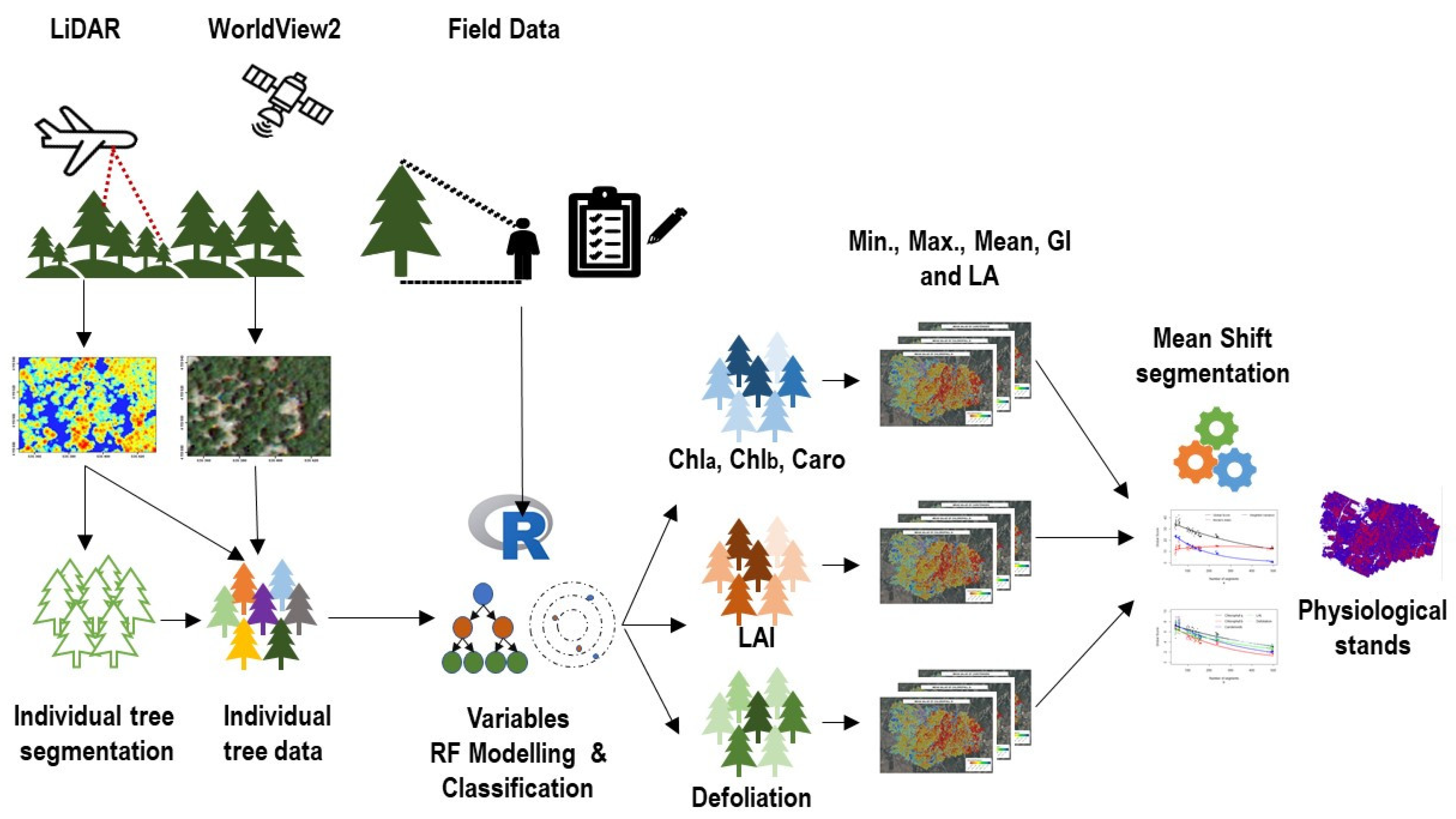
Figure 1. Overview of the proposed workflow to derive stand segmentation based on tree health information from World View-2 multispectral and LiDAR data on southeastern Andalusia Pinus sylvestris forests.
Remotesensing 13 00436 g001
Figure 2. Mean values and standard errors of the LAI and leaf pigments measurements versus crown defoliation in Pinus sylvestris plantations in southern Spain.
Remotesensing 13 00436 g002
Figure 3. Linear regression model between field tree crown delineated of Pinus sylvestris based on pit-free CHM and region growing segmentation algorithm.
Remotesensing 13 00436 g003
Figure 4. Bivariate relationships between imputed and observed chlorophyll content (Chla and Chlb), carotenoids (Car), and LAI estimated by the k-NN imputation using Random Forest distance for regression modeling in Pinus sylvestris plantations at Sierra de los Filabres (Almería, Spain). In all figures, the linear 1:1 line has been fitted. For these equations, the R2 and RMSE values are included.
Remotesensing 13 00436 g004
Figure 5. Behavior of the range radius and minimum region size parameters in the validation score of the segmentations and the number of resulting segments.
Remotesensing 13 00436 g005
Figure 6. Behavior of the Global Score according to the number of segments for (a) Moran’s Index and Weighted Variance, (b) chlorophyll a, chlorophyll b, carotenes, LAI and defoliation, and (c) Gini index (GI), Lorenz asymmetry curve (LAC), maximum (Max), mean (Mean) and minimum (Min) index parameters in the segmentation process.
Remotesensing 13 00436 g006
Figure 7. (a) Stand delineation map obtained using best semi-automatic mean-shift segmentation (Orpheo ToolBox software, OTB) Spatial ratio: 2, range ratio: 0.34, y minimum size: 100. Global Score: 31.83; and (b) Subsets of tree vertical profiles of some transect of stand segmentation area. The map shows the spatial distribution of similar values of severity damages in stands.
Remotesensing 13 00436 g007
Table 1. Silvicultural characteristics of Pinus sylvestris stands in Sierra de los Filabres (Southern Spain). Height (H), basal-area (BA), weighted mean diameter (Dg), Assman dominant height (Ho), density (N), Leaf Area Index (LAI), and pigment content (chlorophyll a and b, Chla and Chlb, and carotenoids Car).
Measured VariablesNo. of obs.MinMeanMaxStDevRangeVariation Coefficient (%)
Pinus sylvestris
H (m)4304.348.6213.021.688.6819.42
Dbh (cm)4308.7018.5030.14.0321.421.79
Ho (m)95.008.1110.101.545.1019.03
BA (m2/ha)918.3326.7140.857.0222.5226.29
N (trees/ha)9509.30952.901405.66296.58896.3631.12
LAI (m2 m−2)450.301.842.820.642.5264.54
Chla (mg g−1)450.031.372.380.672.3549.19
Chlb (mg g−1)450.020.551.020.271.0049.18
Carc (mg g−1)450.010.420.760.200.7549.46
Table 2. World View-2 vegetation indices (VIs) were used as predictor variables for building regression and classification models of defoliation, LAI, and pigments content [48].
AbbreviationNameFormula
Chlorophyll
CSICarter stress indexBand 5/Band 7
NDVINormalized Difference Vegetation Index(Band 7 − Band 5)/(Band 7 + Band 5)
GNDVIGreen Normalized Difference Vegetation Index(Band 7 − Band 3)/(Band 7 + Band 3)
PRIPhotochemical reflectance index(Band 2 − Band 3)/(Band 2 + Band 3)
PSRIPlant Senescence Reflectance Index(Band 5 − Band 2)/Band 6
RENDVIRed Edge Normalized Difference Vegetation Index(Band 7 − Band 6)/(Band 7 + Band 6)
Carotenoid
CRICarotenoid reflectance index(1/Band 3) − (1/Band 6)
Leaf Area Index
NDVINormalized Difference Vegetation Index(Band 7 − Band 5)/(Band 7 + Band 5)
REYRed-Edge Yellow ratio(Band 6 − Band 3)/(Band 6 + Band 3)
Table 3. Severity classes score of individual trees as a function of defoliation percentage and pigment concentration (total Chlorophyll). Severity classes 0: non-damage 1: slight, 2: medium, and 3: High. Adapted from Lakatos et al. [58].
Chlorophyll a + b Concentration (mg/g)
Defoliation >2.02.0 < X < 1.01.0 < X < 0.5<0.5
0–50%10123
50–75%21233
75–100%32333
Table 4. Accuracy assessment of tree delineation using pit-free and region growing segmentation model for all sampled plots of Pinus sylvestris plantations. TP = True Positive, FP = False Positive, FN = False Negative, A = Accuracy in percentage, OE = Omission Error, CE = Commission Error, r = recall, p = precision, F = F-score.
PlotNumber of TreesTPFPFNA (%)OE (%)CE (%)rpF
144421195.452.272.270.980.980.98
254439279.633.7016.670.960.830.89
359485681.3610.178.470.890.910.90
455505090.910.009.091.000.910.95
569618088.410.0011.591.000.880.94
652444484.627.697.690.920.920.92
7252500100.000.000.001.001.001.00
827260196.303.700.000.961.000.98
945360980.0020.000.000.801.000.89
Overall430375322387.215.357.440.940.920.93
Table 5. Variable importance for the selected predictors used as inputs for random forest classification of defoliation and for k-NN modeling using random forest distance for LAI, pigments content, and random forest modeling for defoliation in Pinus sylvestris plantations in Southern Spain. Importance values have been centered and scaled by subtracting the mean value and dividing by its standard deviation. For each tree crown, maximum values in the band 8 of the WorldView2 image (B8_max), mean values in the tree crown in the band 2 (B2_mean), mean values in the band 4 (B4_mean), GNDVI index (GNDVI), percentage of first returns above the 2 m (cov), bincentil 60 (binc60m), mean values in the tree crown in the band 8 (B8_mean), CRI index (CRI), maximum values in the band 5 (B5_max), minimum height of the first returns (zmin1r), minimum values in the band 5 (B5_min), maximum values in the band 2 (B2_max), minimum values in the band 3 (B3_min), percentage of last returns (porclast), maximum values in the band 4 (B4_max), bincentil 40 (binc40), PSRI index (PSRI) were selected.
Chlorophyll aRankScale Importance
PSRI11.584
B4_max21.347
CRI30.436
B8_mean4−0.517
zmin1r5−0.527
binc60m6−0.545
Cov7−0.709
B5_min8−1.068
Chlorophyll bRankScale importance
PSRI11.461
B4_max20.579
CRI30.530
binc60m40.032
B8_mean5−0.165
B5_min6−0.864
B8_max7−1.573
CarotenoidsRankScale importance
B5_min11.293
B8_mean21.205
PSRI30.574
zmin1r40.459
Cov5−0.710
CRI6−0.739
B4_max7−0.796
binc60m8−1.285
LAIRankScale importance
B5_min11.482
B3_min20.366
B5_max3−0.051
CRI4−0.742
B4_min5−1.055
DefoliationRankScale importance
binc4011.281
porclast20.467
B2_max30.248
GNDVI4−0.787
B2_mean5−1.209
Table 6. 10-fold 5-times-repeated cross-validated confusion matrix of random forest classification of defoliation. SLD: Slight level of defoliation; MLD: Moderate level of defoliation; SVD: Severe level of defoliation.
Reference
PredictionCross-Validated DataUser’s
Accuracy
Evaluation DataUser’s
Accuracy
SLDMLDSVDΣSLDMLDSVDΣ
SLD129161015583.2351956578.46
MLD148409885.7153864977.55
SVD70404785.11001616100
Σ15010050 564727
Prod.’s Accuracy868480 91.0780.8559.26
Overall Accuracy84.05 80.77
Kappa0.76 0.69
Publisher’s Note: MDPI stays neutral with regard to jurisdictional claims in published maps and institutional affiliations.