1. Introduction
Thermography allows the measurement of an object’s temperature remotely in a non-invasive way, being its main added value the fact that provides an image instead of a single measurement [
1,
2]. The thermographic camera allows to record the infrared radiation (IR) emitted by bodies as images, and since the emitted radiation is related to the superficial body’s temperature, the IR camera allows the calculation and visualization of the superficial temperature by means of the thermographic images (also called thermograms).
Due to the non-invasive nature of thermography, this has been positioned as a pivotal technique in engineering due to its multiple applications in a large variety of fields [
3,
4,
5,
6]. Not only that, but under the paradigm of the Industry 4.0 revolution, companies are requiring professionals able to apply new procedures to obtain the required flexibility and interoperability [
7]. Therefore, multidisciplinary teaching will improve students’ abilities to face the future challenges [
8]. Thermography is also of interest in predictive maintenance tasks due to the fast transformation of Industry 4.0 [
9]. Moreover, it is susceptible to be combined with machine/deep learning approaches to achieve profitable predictive maintenance as in [
10] where is presented a fuzzy system-based thermography approach for predictive maintenance on electric railways and, also, predictive methods for defect detection in materials [
11].
The use of IR cameras in academic institutions is limited due to their economic cost, which is usually high, and therefore difficult to acquire high-end models due to the budget constraints. However, to specific applications, the low-cost alternatives could be applied [
12]. Examples the of use of IR cameras in the academic context include the visualization of the superficial distribution of engine temperatures [
13], the acquisition of accurate real-time measurements for the analysis and calculation of the different configurations of collectors [
14], as well as a wide range of physics and chemistry experiments, as for example the thermal conductivity and the heat transmission by conduction, energy transformations, the dissipation of mechanical energy and other [
15,
16] and the detection and evaluation of thermal bridges [
17]. Thermography has been also applied has in the training of professionals not directly related to engineering and experimental sciences, for example, for the training of primary teachers in the context of ecocentric education [
18,
19].
Furthermore, the progressive conversion from traditional educational programs to online/asynchronous ones has placed the virtual laboratory paradigm in a pivotal place in engineering programs [
20,
21], especially the development lines related to low-cost implementation and sharing use of resources [
22]. These conversion processes have taken on greater importance in the current context of the pandemic, in which many university programs have switched to e-learning and b-learning.
In this regard, the novel use of 3D visualization software in learning [
23] benefits the students in the acquisition of skills and competences, especially the transversal ones. Please note that this type of software was initially used for tasks related to Geomatics, but the large number of sensors and the development of applications oriented to the three-dimensional reconstruction have increased industrial interest.
In addition to the visualization, students can asynchronously interact with the virtualized learning materials (for example, taking measurements, establishing regions of interest (ROI’s), extracting sections, etc.) thanks to the wide choice of free/open-source visualization software currently available in combination with the remote tutoring of the professor and the support given using Learning Management Systems (LMS) in b-learning and/or e-learning environments.
1.1. Professional Challenges
The acquired competences, abilities, and skills represent the personal qualification to fulfil certain functions in a competent way, related to professional occupation. So, the learning processes should be focused to train the student to become a competent professional. Despite this, not all industrial and productive environment factors can be simulated in the courses, so the practical tasks should be as close as possible to the industrial environment. Furthermore, the professors should assure that the future workers will be prepared to face the Fourth Industrial Revolution, to articulate the knowledge and to learn new technical skills to overcome situations never faced at the training courses [
24].
The present manuscript is focused on a specific issue of this new context, which is the usage of thermographic camera for civil and industrial tasks, which encompass from the detection of anomalies and to the development of simulation models related to obtaining thermal properties such as the emissivity and the heat transfer coefficient, based on thermal gradients, heat distributions, isotherms, and cooling/heating speed. However, more classic applications, such as the use of infrared thermography (IRT) as a visual inspection tool (qualitatively), which is usually employed in the electric systems, predictive maintenance, thermal bridges detection, and other uses. Please note that infrared thermography applied to buildings is not always applied using the passive modality, since in many situations a thermal stimulation of the materials is required; in some cases, the sun is exploited for heating a façade. However, the present teaching-learning activity is based on the passive one, which is the typical one to observe the entire building structure [
25].
The standards developed for the application of infrared thermography in buildings address different issues related to thermal inspection, like BS EN 13187:1999 [
26] which specifies a qualitative method, by thermographic examination, for detecting thermal irregularities in building envelopes; EN ISO 6781-3:2015 [
27] which specifies the qualifications and competence requirements for personnel who perform thermographic investigations on buildings, interpreter the data and report the results; ISO 14683:2017 [
28] which deals with simplified methods for determining heat flows through linear thermal bridges which occur at junctions of building elements, or ASTM E1311 [
29] which refers to the standardized test method for minimum detectable temperature difference for thermal imaging systems. Moreover, it is possible to find in the scientific literature studies related to the application and/or research of thermographic process for building diagnostics. Due to the extent of it, we refer the reader to the next selected articles: A review of the active IR thermography for detection and characterization of defects in reinforced concrete [
30], and a general review of both approaches active/passive [
31,
32].
Some of the main uses of IR images in passive modality are related to the maintenance and inspection tasks. For these, thermography is used to diagnose the buildings/systems, and to schedule the repairs, predict and/or report failures, and/or document its lifecycle. Since the engineers responsible for maintenance works have to base their decisions on the thermographic images, several uncertainties could arise during the image acquisition phase, and therefore they will influence the final decision-making. This need is even more critical when the images are really captured by a maintenance operator without specific knowledge of thermography and infrared radiation, since her/his skill will be another source of uncertainty, as the working environments o the technical specification of the IR camera (also considering the physical difficulty of accessing and inspecting certain machines and devices in complex industrial feasibilities).
By the proposed approach, future engineers could assess the level of uncertainty of the maintenance and inspection tasks, which are related to buildings/systems and other physical parameters as the emissivity since the temperature values obtained using thermography are strongly dependent on the emissivity value of the material [
33], but also other such as humidity, undesired thermal reflections, etc. Thus, this prior small uncertainty could be propagated to the global system, and the combined uncertainty could be increased, causing problems for the interpretation and validation of thermographic images.
1.2. Classical Teaching Apporach
On the classical teaching approach, the relevance of a proper set of the parameters related to temperature (measurement by IR cameras), is exemplified by exercises that follow a structure as follows:
“To determine the superficial temperature of an object, it is considered an emissivity of ε1 = 0.1. As a result, the final temperature is T1 = 150 degC. If the emissivity is really ε2 = 0.2, determine the temperature (T2) and quantify the error.”
Students are taught to use the Stefan-Boltzmann law (1) to relate the temperature change to the fourth power of the emissivity ratio.
Therefore, for this example T2 is equal to 83 degC, being the error committed 67 degC. These kinds of basic examples are very useful for learning about phenomena related to radiation but does not provide insights about the use of IR images in real conditions, and therefore the students’ skills will not be completely developed. This article proposes a new teaching methodology in which the student can discover the limitations of the thermographic technique. This way, in the future, students will be able to know and control all the parameters involved and develop their critical sense to avoid errors derived from an inadequate interpretation of the thermographic image.
Regarding the teaching of thermographic image processing methods, the camera manufacturer’s own software is usually used, which allows changing the colour palette, evaluating trends, working with regions of interest, etc. However, these methods do not specify if the statistics used are useful to evaluate in-depth the temperature and/or infrared radiation variations. Therefore, it is necessary a study of the statistical distributions in thermography so that the student can be critical of the results obtained and the way to interpret them.
1.3. Research Question
For all of the above, the next research question guided the present article: This research aims to evaluate the possible uncertainties in thermographic images. In this way, it will be possible to instruct the students in robust methods that allow obtaining quantitative and qualitative information without committing errors in the interpretation of results.
Therefore, the novelty of the present work is focused on a thermographic approach in the context of education carried out through the application of a workflow based on specific tasks for three-dimensional point clouds processing which have been researched and successfully applied in engineering programs for other issues [
23]. Please note that this approach is not the one usually used in thermography teaching and allows the students to be much more critical with the data to achieve a proper interpretation.
The remainder of the article is structured as follows. In
Section 2 is presented the thermal imaging fundamentals, whereas the design of the learning activity is shown in
Section 3. The output of the activity is presented in
Section 4 in both qualitative and quantitative terms. Lastly,
Section 5 discusses the main conclusions.
2. Theoretical Background
The primary use of IR imaging is the 2D matrixial representation of the temperature distribution of an object’s surface and/or scenario. Despite its usefulness in numerous disciplines, the usage of IR imaging is often reduced to the mere display of the IR image in a qualitative way using a personalized color palette, rather than using the temperature values recorded in the image. Although the use of a color ramp (or color palette) by means of a lookup table enhances the understanding of the underlying information contained in the thermogram, the comparability of the different images is limited by the definition of the lookup table, namely, if the scale is linear or logarithmic, if it is a conventional palette shared by different software or one customized by the user or specifically used by a particular program. Thus, the analysis could be biased, and consequently, the conclusions drawn from the use of the same set of thermal images could differ according to the approach used. In this regard, it is not uncommon to find even analysis based on the digital levels of the color palette in the professional practice. In this regard, students may confuse the “part” with the “whole”. In other words, students may be satisfied with the color information provided by the camera without having critical thinking about what that palette represents, its limitations, and the bias of the capture process.
Consequently, this subsection is dedicated to defining the relationship between the radiance values (collected by the IR camera) and the resulting temperature values, in order to identify the variables that might affect the outcome of the thermographic inspection and bias the subsequent decision-making process. However before that, we need to mention the different IR thermal imaging techniques to put in context the significance of those variables. In this manner, thermal imaging can be categorized as follows [
34]:
Because of the awareness of possible measurement errors in quantitative thermography, it is recommended to use external reference temperature sources, especially with modern cameras based on uncooled detectors [
36]. It is often necessary to use mixed approaches that require both qualitative inspection and qualitative measurement of certain thermal parameters.
The principal parameters that influence the calculation of temperature for passive thermographic inspection are:
Object emissivity.
Relative humidity of the atmosphere.
Projected solid angle. Please note that it, jointly with the detector area (which is a fixed value), can be express as a function of the object distance.
Reflected ambient temperature, or the temperature of the object surroundings.
Atmospheric temperature.
Undesired infrared reflections and shadows in the monitored object can also affect the accuracy of the measurement; however, the effect cannot be quantitatively corrected in an easy and standard way. The camera operator should empirically try to identify such sources and try to vary the perspective to study possible variations in the temperature distribution.
Camera calibration, since there could be calibration shifts due to electronic component aging.
By far, the emissivity is the main feature of the object’s surface, since has an impact on the amount of energy that it is emitted under stationary thermal conditions [
37]. In the case of the analyzed surface has the properties of a blackbody (
BB), it is possible to determine the radiant exitance by means of Planck’s law (2) for a specific wavelength (
λ) and fixed temperature (
T):
where
c1 and
c2 are constants in function of the Planck’s constant (
h), the Boltzmann’s constant (
k), and the velocity of light (
c); whereas
Wλb is the spectral radiant emittance from a blackbody with T temperature at wavelength
λ. Please note that the spectral density cannot be measured for one exact wavelength, since the energy transfer is zero for a single wavelength, it is always measured for a certain wavelength range within the electromagnetic spectrum, which is usually from 8 to 14 microns. Nonetheless, given that real bodies emit only a fraction of the thermal energy (
Wλo) emitted by a blackbody at the same temperature (
Wλb), the final temperature values will be modified. This relationship is related to the emissivity (
ε) as stated in the following Equation (3):
Of all the parameters, emissivity is perhaps one of the most critical [
33] and the most difficult to estimate because it depends on many properties of the object, such as the material, the homogeneity of the object’s surface or the surface finish, the state of deterioration, etc. Despite its relevance in the calculation of temperature, emissivity is a parameter that is often determined with low precision. As a result, the error related to emissivity propagates to the computed superficial temperature of the object, especially when working with absolute temperature values of different objects. In the case of elements with a surface finish with high emissivity values, they will have associated a low reflectance, and therefore, the superficial temperature will be measured easier with the IR camera.
Many non-metallic materials show a high emissivity with a relatively constant trend regardless of their surface characteristics, at least in long-wave spectral ranges (see
Table 1). Countless materials have been differentiated, and their emissivity values are listed in tables like the following:
Please note that the values of
Table 1 are related to a specific ambient temperature, and any temperature change will lead to emissivity changes. They are also based on standard surface conditions. When the surface quality or coating of the material changes, the emissivity value can be different.
The remaining four parameters are linked to the environment and the atmospheric conditions and characterize the atmospheric transmittance. As these variables are measurable up to with certain precision, they will influence temperature calculation (2).
The five aforementioned parameters are the key ones to compute the temperature, but, in a broad vision and according to [
39], they can be complemented with the camera positioning, and in active thermography, also by the intensity, frequency, and the rest of characteristics of the stimulation sources.
The positioning error is of interest when multiple measurements of the same region of interest are carried out. Since this can be minimized by the use of a tripod or another camera fixing system, and the possible position variation for every capture or measurement, this could be dismissed due to the final pixel size (related to the object-sensor distance), this error source will be neglected in the next sections.
Another intrinsic error source that could be taken into account is the one related to the preheating time of the IR camera. The cameras should work at an optimal working temperature, so the acquisition of images without this heating time could generate an error in image series. Since this error source is linked to the proper handle of the camera, it can be considered a gross error, therefore it will be not studied in the following sections.
In the following section, the design of the activity will be described, so that the student can simulate and evaluate the results with a double approach (quantitative and qualitative) under different conditions. Consequently, the student will be able to raise questions, like:
Which would be the most critical atmospheric variable for the study case? or What is the admissible relative error accordingly to the purpose of the thermal inspection?
And derive helpful insights for his/her learning process.
3. Methodology
As stated in the introduction, the focus of the article is the design of a learning activity that will allow the students to understand the uncertainty sources derived from the temperature measurement by means of IR images. The activity is based on the inspection of building facades, since this is important for the training of engineers and one of the most widespread applications of thermography both for inspection and documentation tasks and for energy efficiency tasks. Furthermore, this activity is easy to interpret, with intuitive results, and multidisciplinary useful for various engineers of different specialties. However, firstly, it is necessary to state briefly the typology and characteristics of those measurement errors, which can be random or systematic.
The International Vocabulary of Metrology (VIM) [
40], defines the systematic measurement error as the part of the measurement error that remains constant or varies predictably in replicated measurements, whereas random or Gaussian measurement error is the constituent of the measurement error that varies unpredictably in replicated measurements. Thus, the correction of systematic error sources improves the measurement accuracy, defined as the closeness of agreement among measured quantity values obtained by replicated measurements on the same or similar objects under specified conditions [
40].
The digital levels (DL) obtained from the IR images can be used only for visualization purposes, but not for quantitative thermography, as they are affected by the application of the specific lookup table (color palette) and/or the modification applied over the histogram.
The software supplied by the manufacturer usually allows the measurement of individual temperature values for each pixel. However, such values are influenced by the field parameters of data collection, so they must be adjusted through an adequate analysis and critical reflection made by the students. In other words, the temperature measurement for each point (that is easily extracted from the pixel value of the IR image using manufacturing software) may not be reliable and students should know it.
To facilitate the handling of these error sources, the recorded raw radiance values have to be retrieved from the IR images and stored in an open file format. Thus, it can be manipulated and/or visualized with any scientific software package used in engineering degrees. The IR images, despite being stored in an image compressed format (.jpg), incorporate all the recorded raw radiance values and also the camera metadata needed to calculate the superficial temperatures [
41].
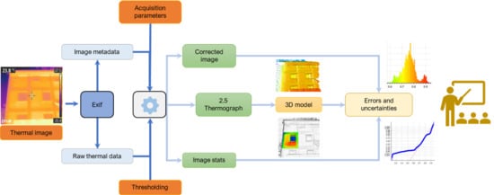
The workflow related to the generation of 3D thermographs and their visualization is shown in
Figure 1:
A specific workflow is used to display the results, which converts the thermograms into 3D viewable models, but with a unique feature: the third axis does not actually represent the elevation, depth, or any metric value, but the temperature of the object surface [
41]. This method has been used with success in the subjects of health sciences degrees for blood flow monitoring and also for emotions [
42].
In the initial phase (
Figure 1), the radiance measurement is extracted (raw) from the images acquired in the field. Thus, the students can manage the calculation of the temperature and modify the error variables. This operation will be supervised by the professor according to the competences to be acquired. The extraction of the raw radiance data can be done with the Exiftool [
43], which is an open-source meta-information reader/writer. This application allows the users to read and modify the EXIF metadata tags of image files, including IR images. By means of a personalized query, it is possible to obtain both the raw digital levels in a 16-bit format and the sensor’s metadata. The latter is highly relevant, and it should be taking into account since it contains the custom sensor’s coefficients necessary for the conversion of the DL to radiance values. Please note that these coefficients are specific for each thermal camera.
After obtaining the recorded radiance values, the calculation of the surface temperature is quite simple through a script on the scientific calculation package. The authors recommend the use of GNU Octave [
44], which is open-source, but more alternatives are available depending on the functionalities supplied as well as the requirement of the teaching, such as Scilab [
45], or Freemat [
46]. At this point, the student or the professor can alter the five input parameters to show the effect on the computation of the final surface temperature, not only numerically but also in terms of its distribution. In addition, it is possible to apply a threshold over the IR image to isolate the significant temperature interval.
The output thermogram remains a 2D image, so it shares the same limitations or interpretation as conventional approaches, for example, the use of unintuitive software to query the surface temperature values of each individual pixel; limited spatial analysis functionalities; or the visualization constrained by the available color palettes. To avoid, or at least minimize, these constraints, the authors propose the use of visualization software from Geomatics engineering. In addition, its suitability in teaching is supported by the argument that the visualization software to be employed by the students has to be open-source (or at least free or free under student license), in order to facilitate its implementation in the teaching strategies and that the student can have the software available anywhere and on any computer. The recommended option is CloudCompare [
47], but as in the preceding case, there are also other free alternatives available, such as Meshlab [
48]. CloudCompare allows 3D editing operations, like measurement, model segmentation and/or sectioning, slicing, adjustment based on parametric surfaces, etc. All these operations can be carried out by the students easily. Moreover, this software offers the professor tools to enhance the visualization of the models such as smooth filters, or the creation of meshes. The goal of the visualization strategy is to facilitate the students the analysis of the thermograph as a 2D entity (like a conventional image) but also as a 3D entity that represents the surface temperature along the third axis.
The activity design was carried out following the three criteria for the creation of virtual models in the context of the virtual environment and virtualization of materials established in previous works [
21,
49], and summarized as quality, economy, and reality criterion. Please note that geometrical precision is not a fundamental parameter to be optimized for this task. However, when performing the thermographic capture is necessary to avoid aberrations or distortions that compromise the geometric fidelity of the objects that appear in the image.
Although these criteria were originally established for the creation of virtual laboratories, given the inherent nature of the current activity, they can be used as guidance for its design and to evaluate the students’ competences [
50]. Therefore, they have been adjusted for the learning objective of the activity (
Table 2):
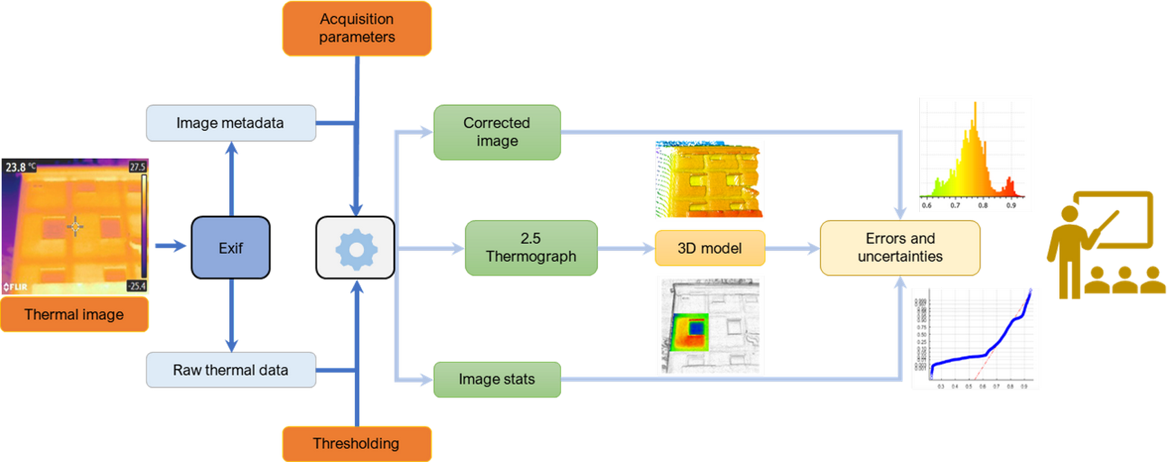
The teaching workflow is structured following the work [
50], and it includes the following steps: Presentation of the activity to the students, theoretical lesson about thermography and aims of the activity; training to use the 3D geomatic visualization software; autonomous and asynchronous work of the students; and finally, the activity submission on the LMS platform. This workflow is summarized in the next figure (
Figure 2):
4. Results
The outcomes of diverse data acquisition configurations can be evaluated by the students in a dual approach: visually (qualitative analysis) and numerically (quantitative analysis). Consequently, students will obtain a more complete vision of the underlying problem of computing temperature from an IR camera (FLIR E6). This thermographic camera was chosen because it is mid-low range, useful for maintenance and evaluation of constructions tasks, and with similar characteristics to the cameras that students could use in their future work.
The camera’s thermal sensitivity if 0.06 degC, whereas the expected accuracy of temperature measurement is ±2 degC or ±2% of reading. Its sensor is a Focal Plane Array, uncooled microbolometer, with a spatial resolution of 5.2 mrad (160 × 120 pixels), capturing radiation between a wavelength of 7.5 µm and 13 µm.
4.1. Qualitative Results
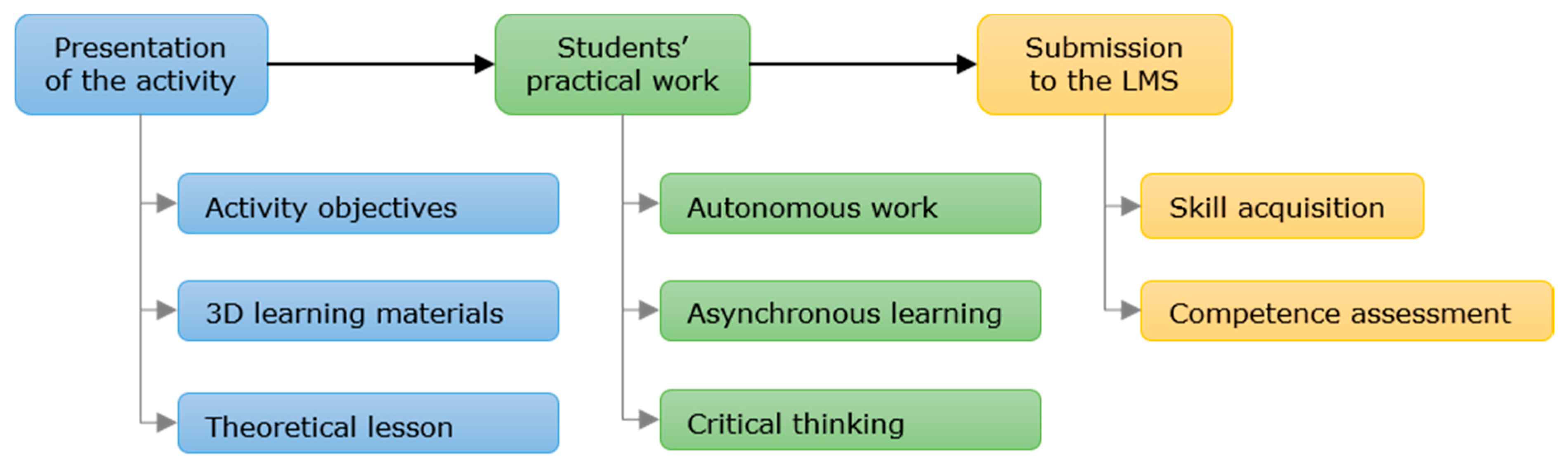
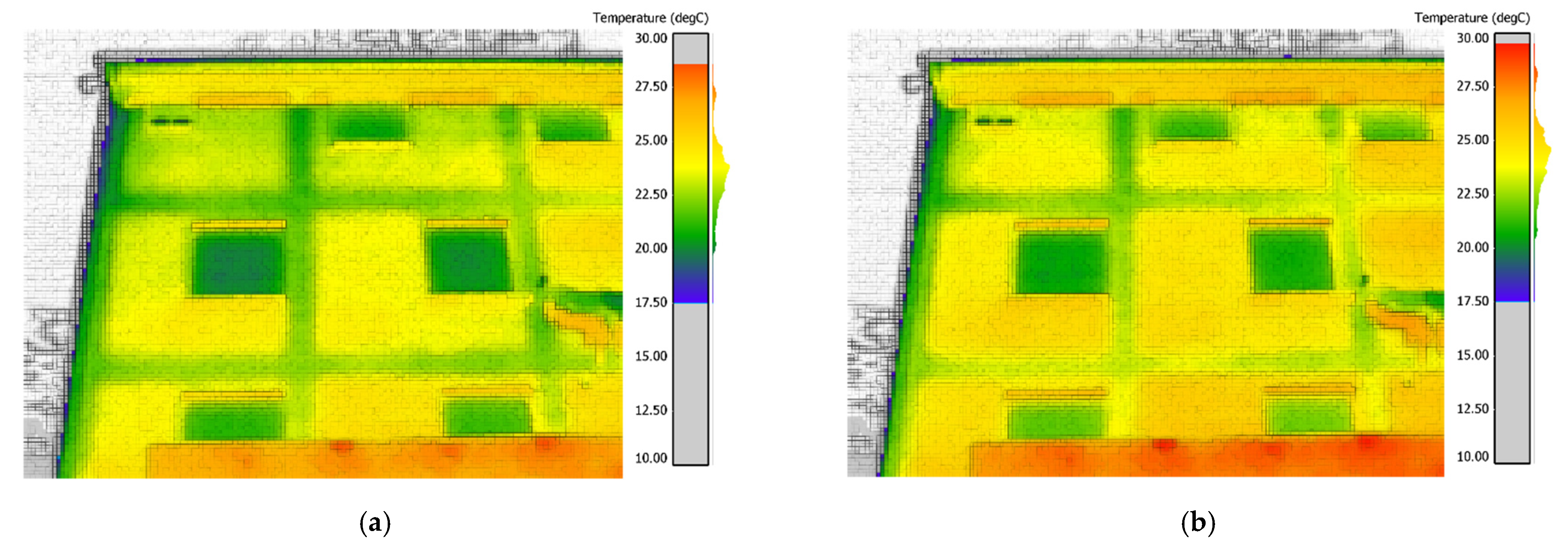
The easiest and most direct approach to interpreting the outcomes is a 3D thermogram as shown in the next figure (
Figure 3). In this Figure it is compared the input IR image with the 3D visualization with a customized color palette. The color palette of the 3D view can be adjusted very easily by the students and does not modify or constraint the query of the superficial temperature.
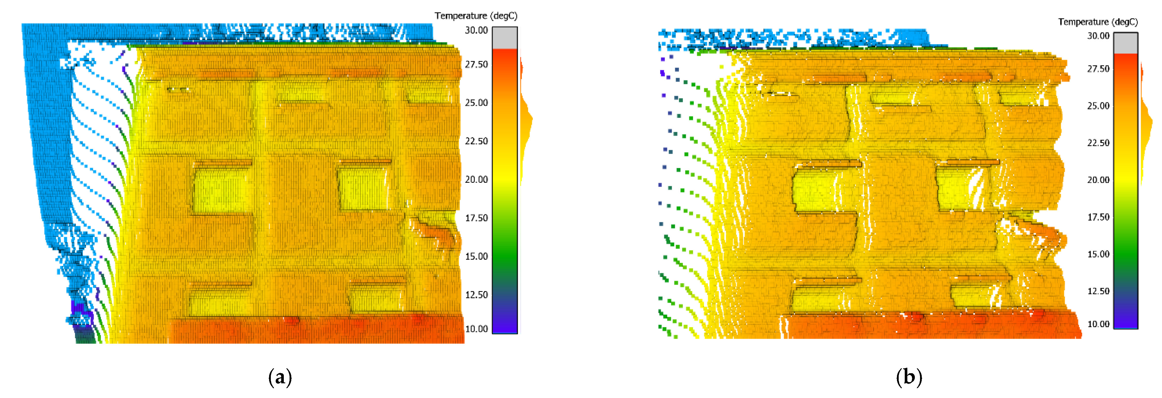
Figure 4a shows the 3D view of the 3D thermogram, whose relief is not the topographical surface of the building but the façade’s surface temperature. Consequently, the student can identify more easily the different areas of contrast and heat exchange. In
Figure 4b the temperature of the same facade is emphasized to highlight the measurement noise as well as the contrast areas. As the reader can appreciate, the first takes a granulated appearance.
Among the tools provided by CloudCompare, it is worth mentioning the Eye-Dome Lighting real-time shader [
51]. Although this plug-in aims to enhance the display of large-scale unorganized point clouds without the need for additional pre-calculation, it can be used to emphasize edges and surface relief (
Figure 5). The third axis, defined orthogonal to the image plane, represents the temperature, and thanks to the aforementioned tool, allow to observe significant local changes in temperature even without the application of a color palette. Furthermore, CloudCompare allows applying a subsampling process in order to remove points in a homogeneous way to generate files with less computational weight, more suitable for the LMS.
The 3D model allows the students to consult interactively the temperature and the position of any point. Given that this 3D thermogram is produced in the absence of any additional data (for example; a range-sensor and/or 3D model of the object/scenario) there is no additional metric information other than the pixel coordinates of the point. These can be transformed into metric units by knowing precisely the distance between the sensor and the façade, but under the hypothesis that the sensor plane is parallel to the façade. The precise scaling of the 3D thermogram is not a priority task for the teaching-learning process, since the present approach can be adapted to multiple kinds of objects and scenarios of the engineering subjects. Among the different tools provided by the visualization, is the option to thresholding the surface temperature values to segment the façade and emphasize the critical areas. Such segmentation is done in a three-dimensional space, so students will also improve the competences related to spatial vision.
4.2. Quantitative Results
The conventional numerical analysis of thermographic images can be 1D as the simple consultation of individual pixel digital values, or 2D analysis like cross-sectional and longitudinal profiles. However, a 3D point cloud has been generated as a novel virtual material from the original IR image, being possible to extend the analysis to illustrate how altering one or more data acquisition variables (object emissivity, atmospheric parameters, object distance, etc.) impacts the computation of temperature, not only numerically, but also spatially. This analysis can be done for the whole study area or to a detailed area to raise the students’ awareness about a determined phenomenon [
52]. In the next figure (
Figure 6) is shown the 3D thermogram of a building façade computed using the correct field values of the aforementioned five parameters (
Figure 6a) and with less accurate ones. The field data acquisition parameters are shown in
Table 3. The computation was carried out according to the pipeline described in
Section 3.
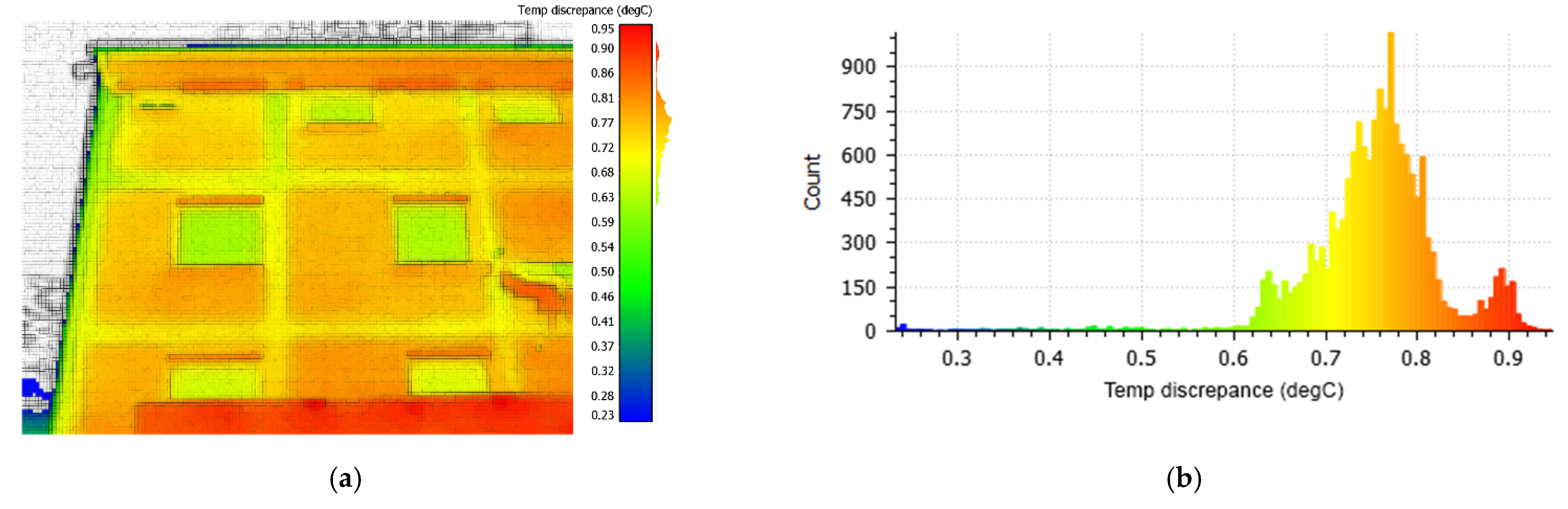
Likewise, it is possible to carry out the operation of map algebra (typical of Geomatics engineering), to subtract the temperature values from the modified 3D thermogram with respect to the one with the correct field data acquisition parameters. This technique is performed with a Geomatic software as CloudCompare [
47]. In
Figure 7a it can be easily seen that the temperature discrepancies are not homogeneous, and they are interrelated with the materials and shape of the façade [
52]. The quantitative overview of the spatial distribution of the temperature differences is depicted as a histogram (
Figure 7b).
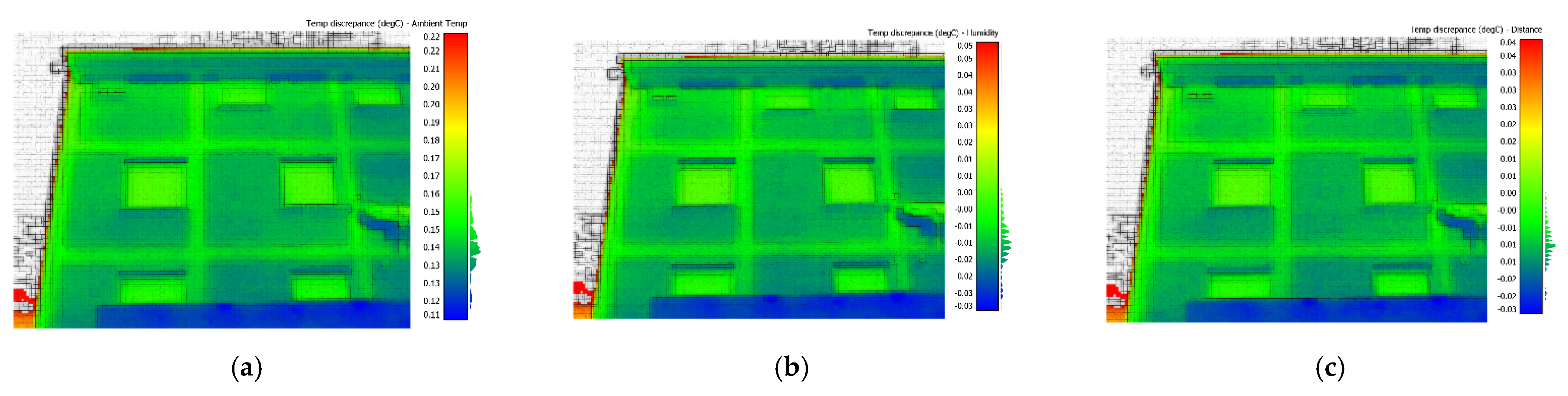
Complementarily it can be studied the individual contribution of different error sources considered. In
Figure 8 it is shown the 3D thermograph for the different data acquisition parameters (
Table 3).
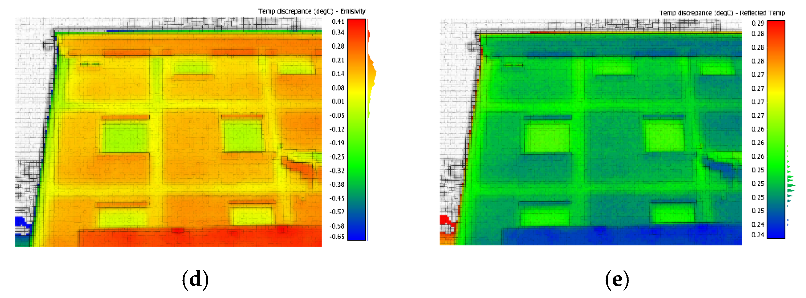
As surface temperature discrepancies are influenced by the specific emissivity values of each patch, their area, and spatial position, the errors will not be random, hence the hypothesis of Gaussian distribution will not be fulfilled. Thus, the customary Gaussian statistical parameters, as the mean and standard deviation, will not represent correctly the multiple error sources and their effect on the final IR image, that is why their use to assess the dispersion and central tendency of the data may not be appropriate. This problem is shown in
Figure 9 both in the histogram and the overlapped Gaussian distribution curve; the Quantile-Quantile (Q-Q) plot; and the Percentile-Percentile (P-P) plot [
53].
Because non-compliance with the assumption of normality will influence the analysis and bias the derived conclusions [
54], a robust statistical approach is presented as part of the activity. In this case, the following robust estimators are adopted in the present study: the median—
m, the normalized median absolute deviation—NMAD (4), the square root of the biweight midvariance—BwMv (5), and the interpercentile ranges (IPR).
Being the median absolute deviation—MAD (8), i.e., the median (
m) of the absolute deviations from the data’s median (
mx):
Therefore, the median is used as a robust measure of the central tendency of thermal discrepancies, whereas the NMAD and the square root of the BwMv as a robust measure of the sample dispersion; instead, the mean and the standard deviation [
55,
56]. As a result, students learn about the non-gaussian statistics and their impact on the final results.
Please note that, for asymmetric distribution, will not be possible to provide a plus-minus range, therefore an absolute inter-percentile range at multiple confidence intervals will be provided (50% also known as the interquartile range, 90%, and 99%), and additionally some percentile values such as 2.5%, 25%, 75%, and 97.5%).
Table 4 presents the parametric and non-parametric statistical results for the façade (
Figure 7a). In the table are listed the individual effects as well as the combined effect of all considered field data acquisition parameters. Please note that, for the present case, the small variation of all parameters shown in
Table 3 can generate a temperature discrepancy circa 0.75 degC (median value) for the façade. Through this kind of analysis, students can assess for each 3D thermograph the effect of the induvial error sources in relation to the nature of the study object. In the case of a painted brick façade, and the parameters shown in
Table 4, the humidity is not a significant one; similarly, the distance due to the short range, and therefore the atmospheric effect. The more significant dispersion generated in the thermographic data is due to the material emissivity (±0.088 degC). In this case, the emissivity values are in the range of the recommended ones by the literature (
Table 4). Therefore, it is shown how for this low-temperature case this effect can overpass the rest for an area of mixed material. Parallelly, the parameters which generated the higher bias in the temperature are the emissivity and ambient temperature parameters. This is an example for the engineering students about advanced statistical concepts like the central tendency (median) and dispersion (e.g., NMAD).
The above table (
Table 4) shows how a modification of the field variables will cause a modification of the façade temperature in a heterogeneous way. This discrepancy will be significant or not according to the final objective of the thermal inspection, which is governed by the teaching subject. Observe that both
Figure 9 and
Table 4 are only a sample of the proposed activity, which can easily be applied to any other object and/or scenario.
Additional multiple values can be derived as the interpercentile ranges (robust and/or Gaussian) for different confidence values (
Table 5). These additional results allow the student to compare the effect of the Gaussian hypothesis in the analysis results.
The Gaussian 99% confidence interval underestimated the robust values by approximately 30% for the present example. For the 95% CI, there is an overestimation of about 10%. This is an example of the teaching of transversal statistical competences for future professionals.
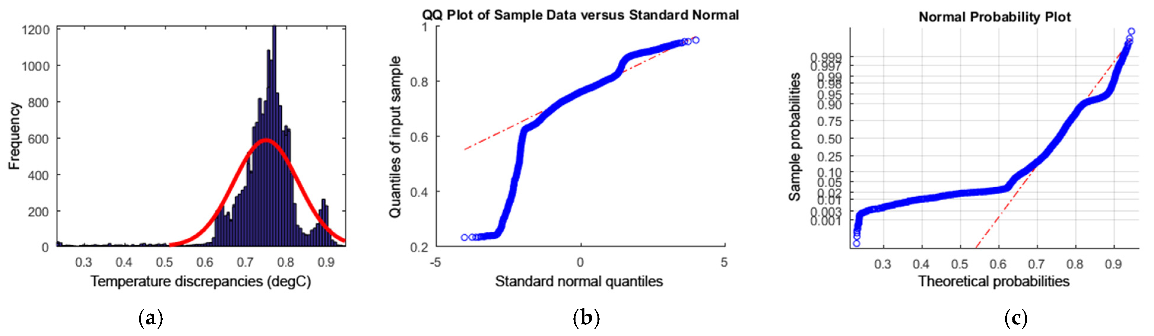
The same virtual material can be segmented into areas of interest for further analysis of the effects of the different uncertainty sources individually or combined (
Figure 10); for example, for the windows where the heat exchange is more significant. Applying the same statistical analysis over the signed thermal discrepancies can be obtained in the summary shown in
Table 6.
Comparing
Table 4 and
Table 6 it is shown that the standard deviation is reduced circa 37% for the detailed area in relation to the complete façade (e.g., 0.080 degC vs. 0.051 degC). However, as shown by the square root of BwMv, this difference is about 11% (e.g., 0.060 degC vs. 0.053 degC). In absolute terms, the thermal difference can be considered no significant, but for the acquisition of competences is relevant, especially for the high-temperature cases, where these discrepancies will be magnified. Real-world data does not usually behave as the parametric models, so the robust statistic will provide correct results even if the conditions are not met exactly. This kind of mathematical skills is very valuable for future professionals to carry out accurate statistical predictions.
Similarly, in
Table 7 are shown the robust and Gaussian interpercentile ranges for different confidence values.
For the detail area, segmented without edge points, it can be shown the effect of Gaussian and robust estimators in the confidence interval, as shown in the table, where for a 99% confidence interval, the difference of temperature discrepancies is overestimated approximately a 41% per the combined case (0.184 degC vs. 0.261 degC). Moreover, in this case, the effect is the contrary to
Table 5 where the Gaussian confidence interval underestimated the values. As a result, the same dataset can be used to teach multiple didactical examples, fulfilling the economic criteria aforementioned [
21,
49].
4.3. Students’ Critical Thinking and Reflections
Finally, based on the statistical results, the students will carry out a reflective task for each study case, based on the results obtained during the process (see
Section 4.1 and
Section 4.2), about the influence of the error sources and requirements of the technique taking into account the objectives of the analysis, being this reflection the meaningful result of the activity.
This reflection will help to develop the students’ critical thinking as well as to complete the acquisition of the subject’s competences. The professor will supervise this task, ensuring the training, and the fulfilling of the learning objectives. In order to encourage the students’ reflection, the session will start with a set of open examples of questions related to the methodology. Next, and in order to illustrate them, there are exemplified some questions:
What are the key objects of the scenario that I have to document?
What is the objective of the final inspection report?
Is it enough to consider the mean and standard deviation to interpret the data?
What statistical parameters are needed to quantitatively assess sources of error?
What are the probable field and meteorological conditions?
What is the anticipated temperature range to be recorded?
Do I need additional instrumentation to ensure adequate quantitative thermographic results? (for example, a thermocouple, a hygrometer).
What should be the frequency of inspection? (number of images and temporal interval).
As a result, there will be a reinforcement of additional skills, as for example critical thinking, statistical concepts, decision making, and problem-solving. Besides, the students will learn the benefits of using software from other disciplines, as geomatics engineering, and to adapt to their needs. Students could also fulfill a table (
Table 8) similar to the next one, obtained from [
39]:
5. Conclusions
A procedure for thermographic image analysis using geomatic software has been presented. This procedure allows a more critical evaluation of the parameters involved in thermography and applies to the models’ statistical processing that allows seeing the distribution of data and the presence of biases or non-normalities. The research has been implemented using open software, and the activity can be integrated into e-learning or b-learning educational programs.
As a result of the pandemic situation, the number of programs available online in higher education is growing, but it remains a challenge to generate quality learning materials to transform traditional teaching into new degrees, focusing on case studies and meaningful career-related activities. In particular, the focus of this manuscript is to contribute to the creation of a series of participatory activities in subjects associated with IR imaging to stimulate critical thinking in students, in relation to the IR error sources and their consequences and variability. Collaterally, mathematical and statistical skills are also reinforced.
The final objective of this manuscript is to introduce a dynamic and comprehensive pipeline for the acquisition and development of advanced skills derived from the use of thermographic images as 3D models and the knowledge of the main sources of uncertainty. With this activity students can be introduced to the physical phenomena of heat transfer using thermography, as it has been proposed in other works at different educational levels [
15,
16]. Specifically, this work proposes the use of robust statistics applied on thermographic images with geomatic techniques that, as the results show, can ’unmask’ false results derived from the application of classical parametric statistics and this can be used as a teaching potential.
Furthermore, the proposed method is low cost by emphasizing the use of open/free Geomatics software (CloudCompare) for visualization purposes and mathematical package for the mathematical conversion (Octave), both free, and that can be used both in engineering science programs, and by the student himself; unlike the infrared camera, which if it is a piece of expensive equipment, but as it is only necessary to collect the thermal images of the objects of interest to the subject. Please note, that there are also low-cost thermal imaging devices that can be used paired to a smartphone as an acceptable substitute.
The present analysis of thermographic images is highly specialized, being especially useful for engineering students familiar with rescaling of thermographic images and statistical analysis. Moreover, the activity will be specifically designed to show the importance of robust statistics and to show the student the limitations of the parametric statistics that they commonly use in other tasks. The shown case study is the monitoring of a facade for the study of heat distribution and thermal bridges. However, this methodology would be applicable to any thermographic image used in inspection and maintenance tasks (e.g., electrical systems, engines, fluid installations, etc.). As the radiation comes from the object and different sources, outliers can appear, which implies that students are only able to extract a general opinion. So, the possible presence of systematisms, and/or outliers detected in the experiments carried out, will hinder the use of Gaussian statistics like the mean and the standard deviation, since they will not always provide a suitable analysis, therefore the transversal statistical competence will benefit students’ critical thinking.
Given the multidisciplinary and novel nature of the infrared thermography technique, its experimental application could be included in different engineering programs, by explaining and understanding abstract theoretical concepts in class as well as e-learning methods, thus helping students to be better prepared to face the challenges of the Industry 4.0. Furthermore, this resource can be integrated within e-learning and b-learning methodologies.
Once it has been demonstrated the possibility of working with 3D models obtained from thermal imaging and with robust statistics in order to detect and evaluate possible errors, future works could include the experimental application of this technique in students from different engineering programs, given the multidisciplinary nature of the thermographic technique.


