
Feasibility of Ground-Based Sky-Camera HDR Imagery to Determine Solar Irradiance and Sky Radiance over Different Geometries and Sky Conditions

 , ,
, ,
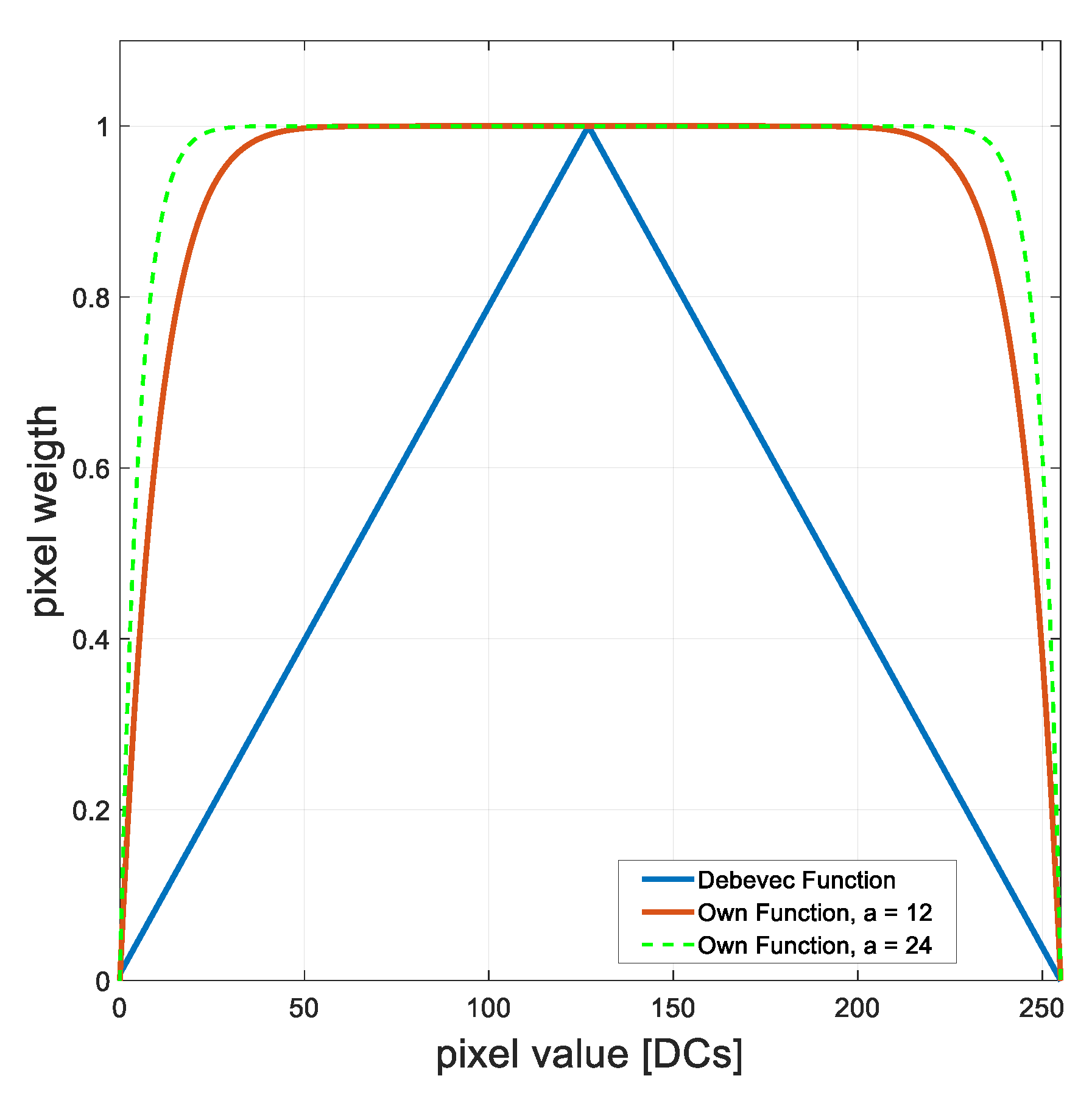
Abstract
:
1. Introduction
2. Site Measurements and Data
3. Characterization of the SONA Sky-Camera
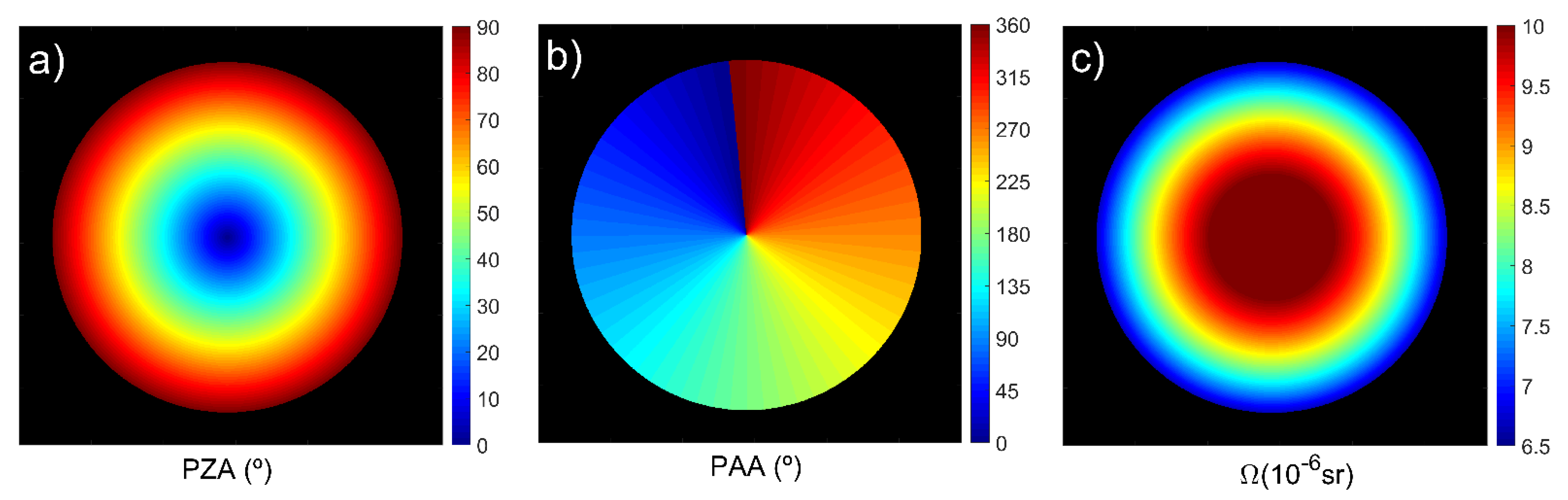
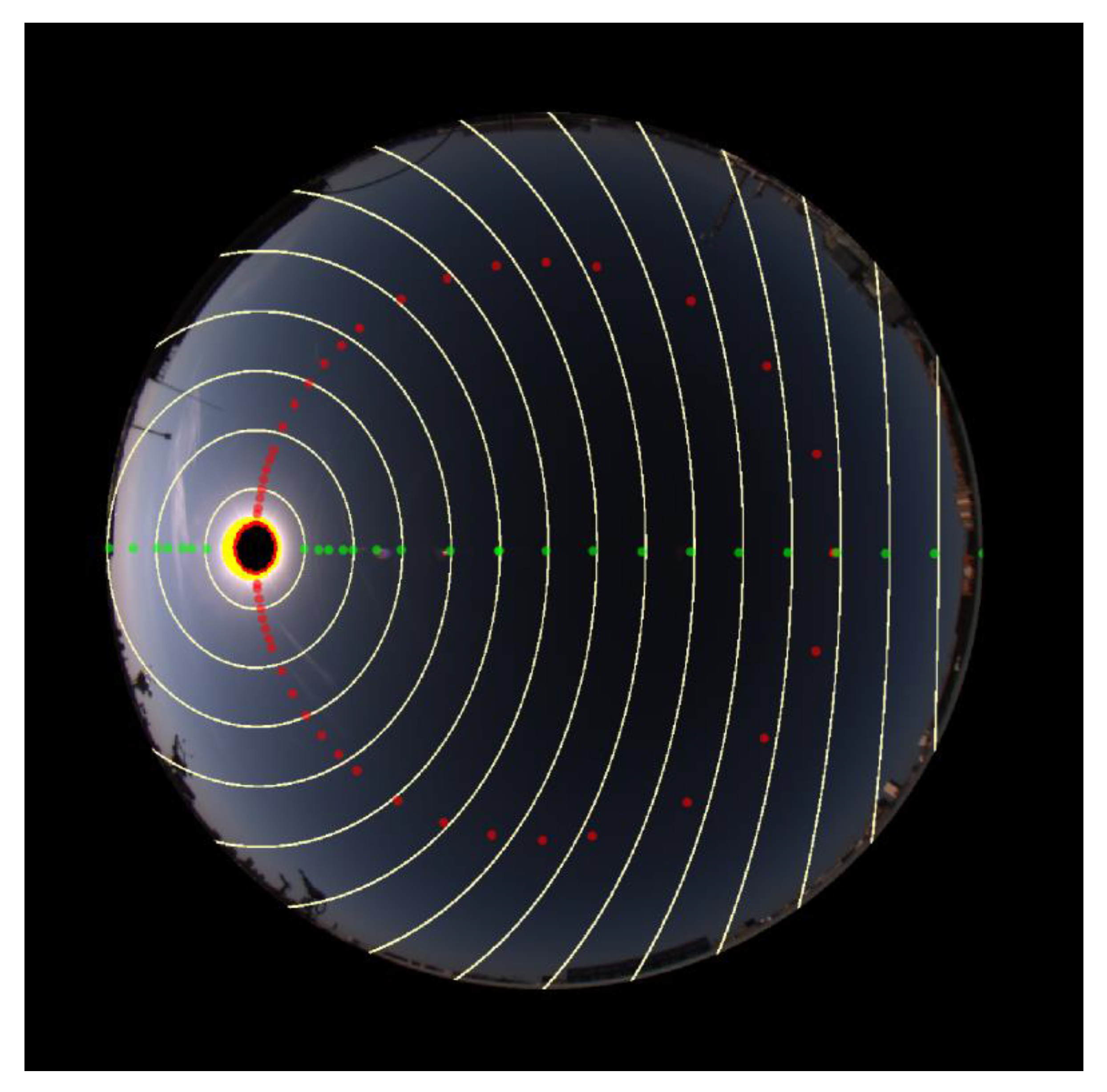
3.1. Geometric Calibration
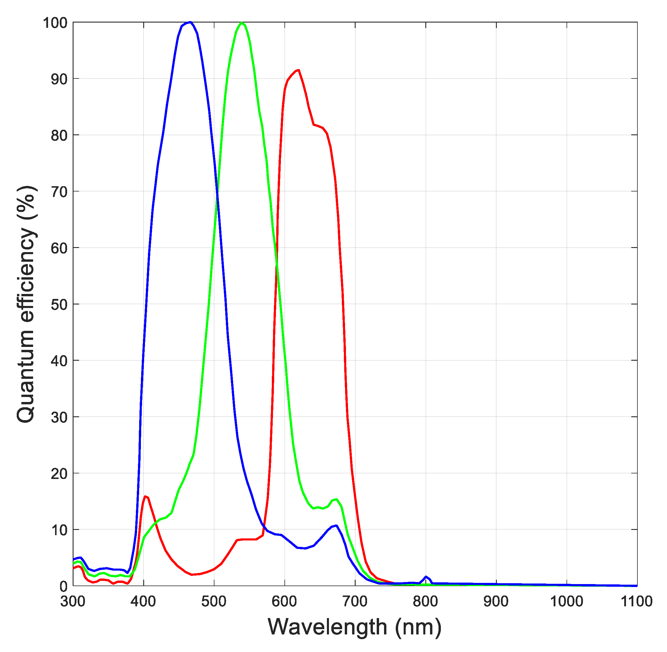
3.2. Sensor Characterization
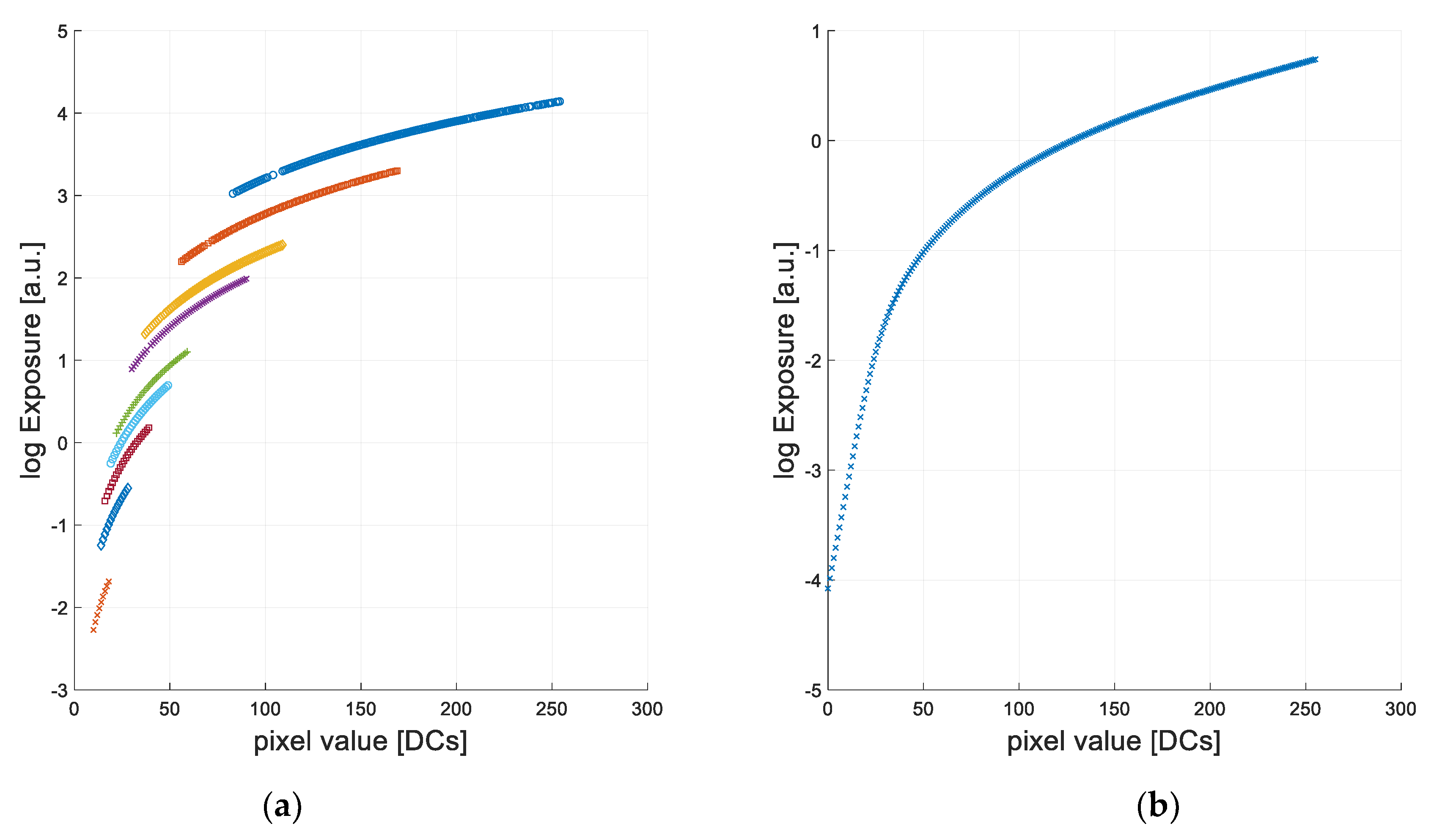
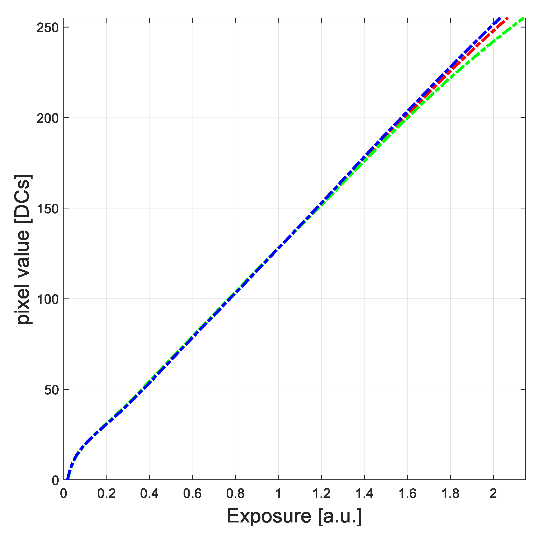
3.3. Camera Response Function
3.4. Constructing the High Dynamic Range Imagery
3.5. Radiometric Calibration
4. Methods to Obtain Solar Radiation
4.1. Determination of the Sky-Radiance
4.2. Broadband Diffuse Irradiance on a Horizontal Plane
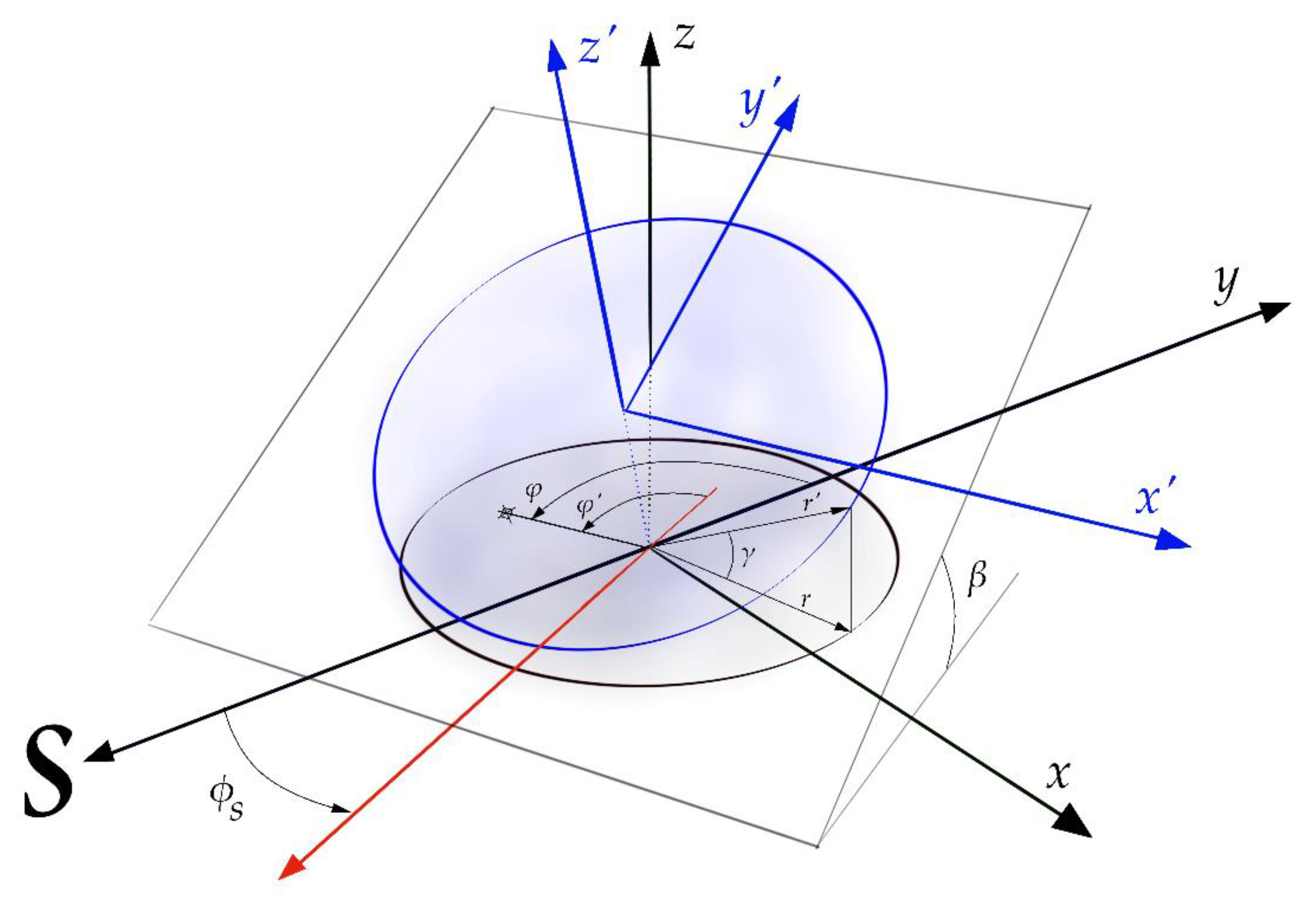
4.3. Broadband Diffuse Irradiance on Arbitrary Planes
5. Results
5.1. Validation of Sky Radiance
5.2. Determination of Broadband Horizontal Diffuse Irradiance
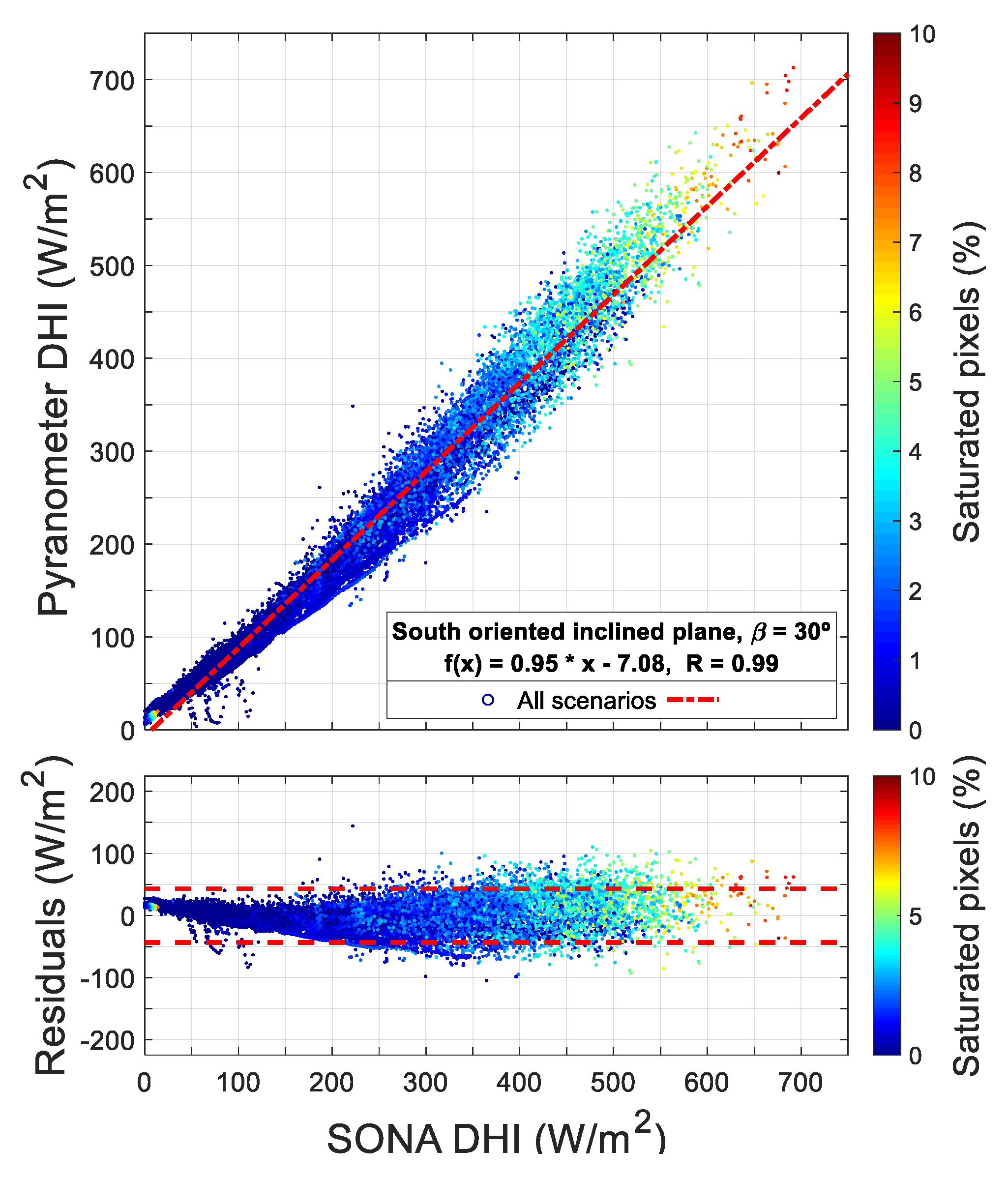
5.3. Validation of Broadband Diffuse on an Arbitrarily Oriented Plane
6. Conclusions
Supplementary Materials
Author Contributions
Funding
Institutional Review Board Statement
Informed Consent Statement
Data Availability Statement
Conflicts of Interest
References
- IEA. World Energy Outlook 2017; International Energy Agency and Organisation for Economic Co-operation and Development OECD: Paris, France, 2017; ISBN 978-92-64-28230-8. [Google Scholar]
- Tsiropoulos, I.; Nijs, W.; Tarvydas, D.; Ruiz Castello, P. Towards Net-Zero Emissions in the EU Energy System by 2050; EUR 29981 EN; Publications Office of the European Union: Luxembourg, 2020; ISBN 978-92-76-13096-3. [Google Scholar] [CrossRef]
- Crook, J.A.; Jones, L.A.; Forster, P.M.; Crook, R. Climate change impacts on future photovoltaic and concentrated solar power energy output. Energy Environ. Sci. 2011, 4, 3101–3109. [Google Scholar] [CrossRef]
- Gaetani, M.; Huld, T.; Vignati, E.; Monforti-Ferrario, F.; Dosio, A.; Raes, F. The near future availability of photovoltaic energy in Europe and Africa in climate-aerosol modeling experiments. Renew. Sustain. Energy Rev. 2014, 38, 706–716. [Google Scholar] [CrossRef]
- Nieto, J.; Carpintero, O.; Lobejón, L.F.; Miguel, L.J. An ecological macroeconomics model: The energy transition in the EU. Energy Policy 2020, 145, 111726. [Google Scholar] [CrossRef]
- Alonso-Montesinos, J.; Batlles, F.; Portillo, C. Solar irradiance forecasting at one-minute intervals for different sky conditions using sky camera images. Energy Convers. Manag. 2015, 105, 1166–1177. [Google Scholar] [CrossRef]
- Ohmura, A.; Gilgen, H.; Hegner, H.; Müller, G.; Wild, M.; Dutton, E.G.; Forgan, B.; Fröhlich, C.; Philipona, R.; Heimo, A.; et al. Baseline Surface Radiation Network (BSRN/WCRP): New Precision Radiometry for Climate Research. Bull. Am. Meteorol. Soc. 1998, 79, 2115–2136. [Google Scholar] [CrossRef] [Green Version]
- Nowak, D.; Vuilleumier, L.; Long, C.N.; Ohmura, A. Solar irradiance computations compared with observations at the Baseline Surface Radiation Network Payerne site. J. Geophys. Res. Space Phys. 2008, 113. [Google Scholar] [CrossRef] [Green Version]
- Long, C.N.; Ackerman, T.P. Identification of clear skies from broadband pyranometer measurements and calculation of downwelling shortwave cloud effects. J. Geophys. Res. Space Phys. 2000, 105, 15609–15626. [Google Scholar] [CrossRef]
- Barnard, J.C.; Long, C.N. A Simple Empirical Equation to Calculate Cloud Optical Thickness Using Shortwave Broadband Measurements. J. Appl. Meteorol. 2004, 43, 1057–1066. [Google Scholar] [CrossRef] [Green Version]
- Long, C.N.; Ackerman, T.P.; Gaustad, K.L.; Cole, J.N.S. Estimation of fractional sky cover from broadband shortwave radiometer measurements. J. Geophys. Res. Space Phys. 2006, 111. [Google Scholar] [CrossRef] [Green Version]
- Ridley, B.; Boland, J.; Lauret, P. Modelling of diffuse solar fraction with multiple predictors. Renew. Energy 2010, 35, 478–483. [Google Scholar] [CrossRef]
- Aler, R.; Galvan, I.M.; Ruiz-Arias, J.A.; Gueymard, C.A. Improving the separation of direct and diffuse solar radiation components using machine learning by gradient boosting. Sol. Energy 2017, 150, 558–569. [Google Scholar] [CrossRef]
- Perez, R.; Lorenz, E.; Pelland, S.; Beauharnois, M.; Van Knowe, G.; Hemker, K.; Heinemann, D.; Remund, J.; Müller, S.C.; Traunmüller, W.; et al. Comparison of numerical weather prediction solar irradiance forecasts in the US, Canada and Europe. Sol. Energy 2013, 94, 305–326. [Google Scholar] [CrossRef]
- Camargo, L.R.; Dorner, W. Comparison of satellite imagery based data, reanalysis data and statistical methods for mapping global solar radiation in the Lerma Valley (Salta, Argentina). Renew. Energy 2016, 99, 57–68. [Google Scholar] [CrossRef]
- Kim, C.K.; Kim, H.-G.; Kang, Y.-H.; Yun, C.-Y.; Lee, Y.G. Intercomparison of Satellite-Derived Solar Irradiance from the GEO-KOMSAT-2A and HIMAWARI-8/9 Satellites by the Evaluation with Ground Observations. Remote Sens. 2020, 12, 2149. [Google Scholar] [CrossRef]
- Cristóbal, J.; Anderson, M.C. Validation of a Meteosat Second Generation solar radiation dataset over the northeastern Iberian Peninsula. Hydrol. Earth Syst. Sci. 2013, 17, 163–175. [Google Scholar] [CrossRef] [Green Version]
- Greuell, W.; Meirink, J.F.; Wang, P. Retrieval and validation of global, direct, and diffuse irradiance derived from SEVIRI satellite observations. J. Geophys. Res. Atmos. 2013, 118, 2340–2361. [Google Scholar] [CrossRef]
- Alonso-Montesinos, J.; Batlles, F. The use of a sky camera for solar radiation estimation based on digital image processing. Energy 2015, 90, 377–386. [Google Scholar] [CrossRef]
- Mejia, F.A.; Kurtz, B.; Murray, K.; Hinkelman, L.M.; Sengupta, M.; Xie, Y.; Kleissl, J. Coupling sky images with radiative transfer models: A new method to estimate cloud optical depth. Atmos. Meas. Tech. 2016, 9, 4151–4165. [Google Scholar] [CrossRef] [Green Version]
- Lothon, M.; Barnéoud, P.; Gabella, O.; Lohou, F.; Derrien, S.; Rondi, S.; Chiriaco, M.; Bastin, S.; Dupont, J.C.; Haeffelin, M.; et al. ELIFAN, an algorithm for the estimation of cloud cover from sky imagers. Atmos. Meas. Tech. 2019, 12, 5519–5534. [Google Scholar] [CrossRef] [Green Version]
- Xie, W.; Liu, D.; Yang, M.; Chen, S.; Wang, B.; Wang, Z.; Xia, Y.; Liu, Y.; Wang, Y.; Zhang, C. SegCloud: A novel cloud image segmentation model using a deep convolutional neural network for ground-based all-sky-view camera observation. Atmos. Meas. Tech. 2020, 13, 1953–1961. [Google Scholar] [CrossRef] [Green Version]
- Román, R.; Antón, M.; Cazorla, A.; de Miguel, A.; Olmo, F.J.; Bilbao, J.; Alados-Arboledas, L. Calibration of an all-sky camerasky-camera for obtaining sky-radiance at three wavelengths. Atmos. Meas. Tech. 2012, 5, 2013–2024. [Google Scholar] [CrossRef] [Green Version]
- Cazorla, A.; Olmo, F.; Alados-Arboledas, L.; Reyes, F.J.O. Using a Sky Imager for aerosol characterization. Atmos. Environ. 2008, 42, 2739–2745. [Google Scholar] [CrossRef]
- Ghonima, M.S.; Urquhart, B.; Chow, C.W.; Shields, J.E.; Cazorla, A.; Kleissl, J. A method for cloud detection and opacity classification based on ground based sky imagery. Atmos. Meas. Tech. 2012, 5, 2881–2892. [Google Scholar] [CrossRef] [Green Version]
- Román, R.; Torres, B.; Fuertes, S.; Cachorro, V.E.; Dubovik, O.; Toledano, C.; Cazorla, A.; Barreto, A.; Bosch, J.L.; Lapyonok, T.; et al. Remote sensing of lunar aureole with a sky camera: Adding information in the nocturnal retrieval of aerosol properties with GRASP code. Remote Sens. Environ. 2017, 196, 238–252. [Google Scholar] [CrossRef] [Green Version]
- Román, R.; Antuña-Sánchez, J.C.; Cachorro, V.E.; Toledano, C.; Torres, B.; Mateos, D.; Fuertes, D.; López, C.; González, R.; Lapionok, T.; et al. Retrieval of aerosol properties using relative radiance measurements from an all-sky camera. Atmos. Meas. Tech. Discuss. 2021. [Google Scholar] [CrossRef]
- Chu, Y.; Pedro, H.; Li, M.; Coimbra, C.F. Real-time forecasting of solar irradiance ramps with smart image processing. Sol. Energy 2015, 114, 91–104. [Google Scholar] [CrossRef]
- Kurtz, B.; Kleissl, J. Measuring diffuse, direct, and global irradiance using a sky imager. Sol. Energy 2017, 141, 311–322. [Google Scholar] [CrossRef]
- Scolari, E.; Sossan, F.; Haure-Touzé, M.; Paolone, M. Local estimation of the global horizontal irradiance using an all-sky camera. Sol. Energy 2018, 173, 1225–1235. [Google Scholar] [CrossRef]
- Estellés, V.; Martínez-Lozano, J.A.; Utrillas, M.P.; Campanelli, M. Columnar aerosol properties in Valencia (Spain) by ground-based Sun photometry. J. Geophys. Res. 2007, 112, D11201. [Google Scholar] [CrossRef] [Green Version]
- Segura, S.; Estellés, V.; Esteve, A.; Marcos, C.; Utrillas, M.; Martínez-Lozano, J. Multiyear in-situ measurements of atmospheric aerosol absorption properties at an urban coastal site in western Mediterranean. Atmos. Environ. 2016, 129, 18–26. [Google Scholar] [CrossRef]
- Marcos, C.R.; Gómez-Amo, J.L.; Péris, C.; Pedrós, R.; Utrillas, M.P.; Martínez-Lozano, J.A. Analysis of four years of ceilometer-derived aerosol backscatter profiles in a coastal site of the western Mediterranean. Atmos. Res. 2018, 213, 331–345. [Google Scholar] [CrossRef]
- Gómez-Amo, J.L.; Estellés, V.; Marcos, C.; Segura, S.; Esteve, A.R.; Pedrós, R.; Utrillas, M.P.; Martínez-Lozano, J.A. Impact of dust and smoke mixing on column-integrated aerosol properties from observations during a severe wildfire episode over Valencia (Spain). Sci. Total Environ. 2017, 599–600, 2121–2134. [Google Scholar] [CrossRef]
- Gómez-Amo, J.; Freile-Aranda, M.; Camarasa, J.; Estellés, V.; Utrillas, M.; Martínez-Lozano, J. Empirical estimates of the radiative impact of an unusually extreme dust and wildfire episode on the performance of a photovoltaic plant in Western Mediterranean. Appl. Energy 2018, 235, 1226–1234. [Google Scholar] [CrossRef]
- Holben, B.N.; Eck, T.F.; Slutsker, I.; Tanré, D.; Buis, J.P.; Setzer, A.; Vermote, E.; Reagan, J.A.; Kaufman, Y.J.; Nakajima, T.; et al. AERONET—A Federated Instrument Network and Data Archive for Aerosol Characterization. Remote Sens. Environ. 1998, 66, 1–16. [Google Scholar] [CrossRef]
- Estellés, V.; Campanelli, M.; Smyth, T.J.; Utrillas, M.P.; Martínez-Lozano, J.A. AERONET and ESR sun direct products comparison performed on Cimel CE318 and Prede POM01 solar radiometers. Atmos. Chem. Phys. 2012, 12, 11619–11630. [Google Scholar] [CrossRef] [Green Version]
- Dubovik, O.; Holben, B.; Eck, T.F.; Smirnov, A.; Kaufman, Y.J.; King, M.D.; Tanré, D.; Slutsker, I. Variability of absorption and optical properties of key aerosol types observed in worldwide locations. J. Atmos. Sci. 2002, 59, 590–608. [Google Scholar] [CrossRef]
- Ma, C.; Arias, E.F.; Eubanks, T.M.; Fey, A.L.; Gontier, A.-M.; Jacobs, C.S.; Sovers, O.J.; Archinal, B.A.; Charlot, P. The International Celestial Reference Frame as Realized by Very Long Baseline Interferometry. Astron. J. 1998, 116, 516–546. [Google Scholar] [CrossRef]
- Cox, W. The theory of perspective. Br. J. Photogr. 1969, 116, 628–659. [Google Scholar]
- Debevec, P.E.; Malik, J. Recovering high dynamic range radiance maps from photographs. SIGGRAPH 2003, 1, 374–380. [Google Scholar] [CrossRef]
- Mitsunaga, T.; Nayar, S. Radiometric self calibration. In Proceedings of the 1999 IEEE Computer Society Conference on Computer Vision and Pattern Recognition (Cat. No PR00149), Fort Collins, CO, USA, 23–25 June 1999; Volume 1, pp. 374–380. [Google Scholar] [CrossRef]
- Antuña-Sánchez, J.C.; Román, R.; Cachorro, V.E.; Toledano, C.; López, C.; González, R.; Mateos, D.; Calle, A.; de Frutos, Á.M. Relative sky-radiance from multi-exposure all-sky camerasky-camera images. Atmos. Meas. Tech. 2021, 14, 2201–2217. [Google Scholar] [CrossRef]
- Emde, C.; Buras-Schnell, R.; Kylling, A.; Mayer, B.; Gasteiger, J.; Hamann, U.; Kylling, J.; Richter, B.; Pause, C.; Dowling, T.; et al. The libRadtran software package for radiative transfer calculations (version 2.0.1). Geosci. Model Dev. 2016, 9, 1647–1672. [Google Scholar] [CrossRef] [Green Version]
- Kholopov, G.K. Calculation of the effective wavelength of a measuring system. J. Appl. Spectrosc. 1975, 23, 1146–1147. [Google Scholar] [CrossRef]
- Henyey, L.C.; Greenstein, J.L. Diffuse radiation in the Galaxy. Astrophys. J. 1941, 93, 70–83. [Google Scholar] [CrossRef]
- Vermeulen, A. Caractérisation des Aérosols á Partir de Mesures Optiques Passives au Sol: Apport des Luminances Totale et Polarisée Mesurées dans le Plan Principal. Ph.D. Thesis, Université de Lille, Lille, France, 1996. [Google Scholar]
- Torres, B.; Toledano, C.; Berjón, A.; Fuertes, D.; Molina, V.; González, R.; Canini, M.; Cachorro, V.E.; Goloub, P.; Podvin, T.; et al. Measurements on pointing error and field of view of Cimel-318 Sun photometers in the scope of AERONET. Atmos. Meas. Tech. 2013, 6, 2207–2220. [Google Scholar] [CrossRef] [Green Version]
- Blanc, P.; Espinar, B.; Geuder, N.; Gueymard, C.; Meyer, R.; Pitz-Paal, R.; Reinhardt, B.; Renné, D.; Sengupta, M.; Wald, L.; et al. Direct normal irradiance related definitions and applications: The circumsolar issue. Sol. Energy 2014, 110, 561–577. [Google Scholar] [CrossRef]
- Major, G. Estimation of the error caused by the circumsolar radiation when measuring global radiation as a sum of direct and diffuse radiation. Sol. Energy 1992, 48, 249–252. [Google Scholar] [CrossRef]


| Centre | |||||
|---|---|---|---|---|---|
| Fisheye Projection | f (µm) | X ± 2 | Y ± 2 | R2 | |
| Equidistant | 0.84 | 577 | 584 | 1.0 | |
| Orthographic | 0.01 | 594 | 572 | 0.8 | |
| Stereographic | 0.02 | 576 | 589 | 0.9 | |
| Wavelength (nm) | λeff ± 1 σ(nm) |
|---|---|
| Blue | 480 ± 6 |
| Green | 541 ± 5 |
| Red | 615 ± 6 |
| λ (nm) | Relative Uncertainty (%) | |
|---|---|---|
| 480 | 0.26 ± 0.02 | 7% |
| 541 | 0.34 ± 0.02 | 7% |
| 615 | 0.50 ± 0.05 | 10% |
| Clear Sky | Partially Cloudy Sky | All Scenarios | ||||||||||
|---|---|---|---|---|---|---|---|---|---|---|---|---|
| λ | RMBD | CL10 | N | R | RMBD | CL10 | N | R | RMBD | CL10 | N | R |
| (nm) | (%) | (%) | (#) | (#) | (%) | (%) | (#) | (#) | (%) | (%) | (#) | (#) |
| 675 | 9 | 91 | 12,680 | 0.96 | 28 | 42 | 36,279 | 0.81 | 23 | 51 | 48,959 | 0.82 |
| 500 | 6 | 85 | 8720 | 0.98 | 10 | 75 | 23,116 | 0.92 | 8 | 79 | 31,836 | 0.93 |
| 440 | 4 | 91 | 12,320 | 0.98 | 10 | 76 | 35,513 | 0.90 | 8 | 81 | 47,833 | 0.91 |
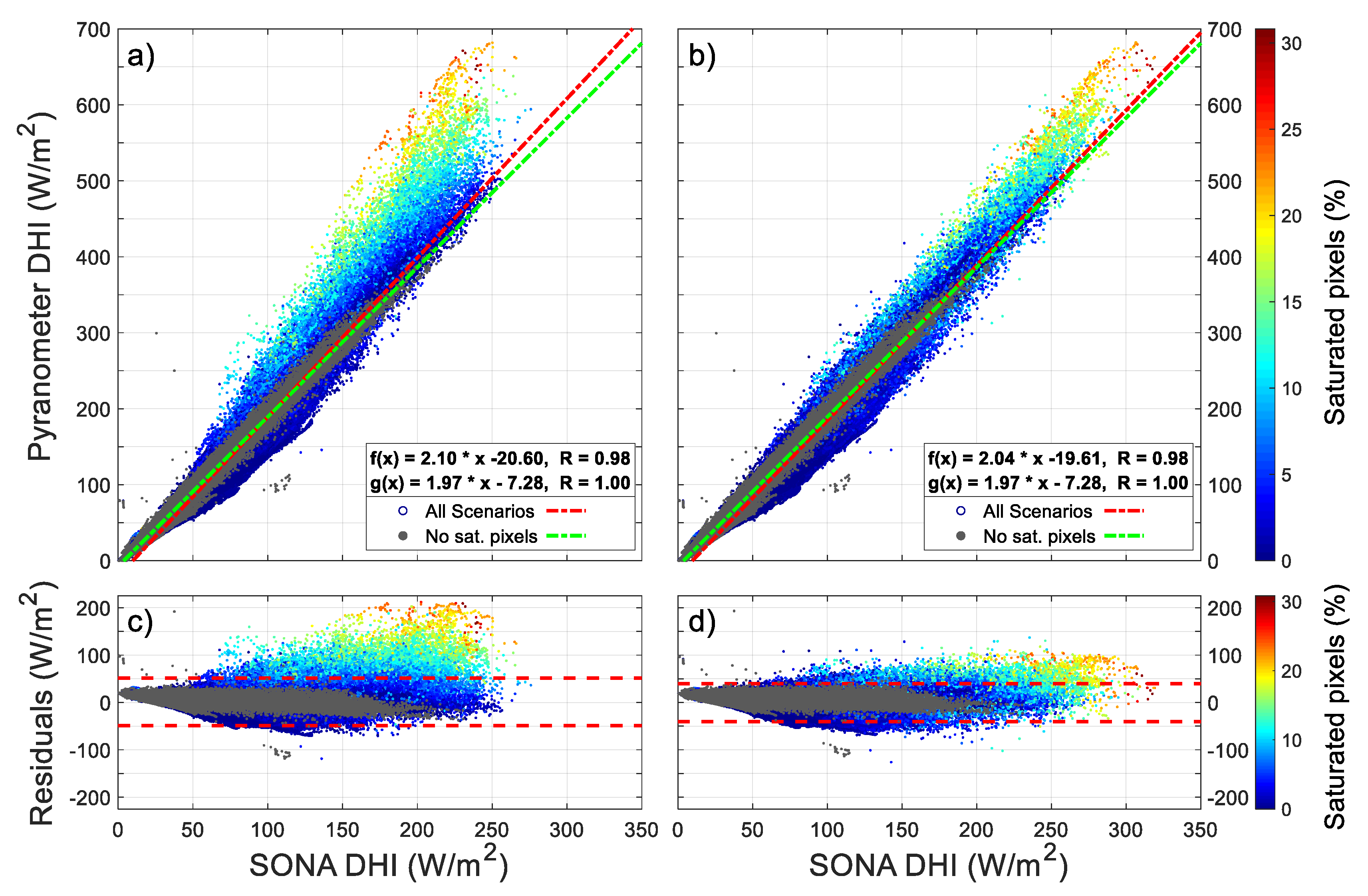
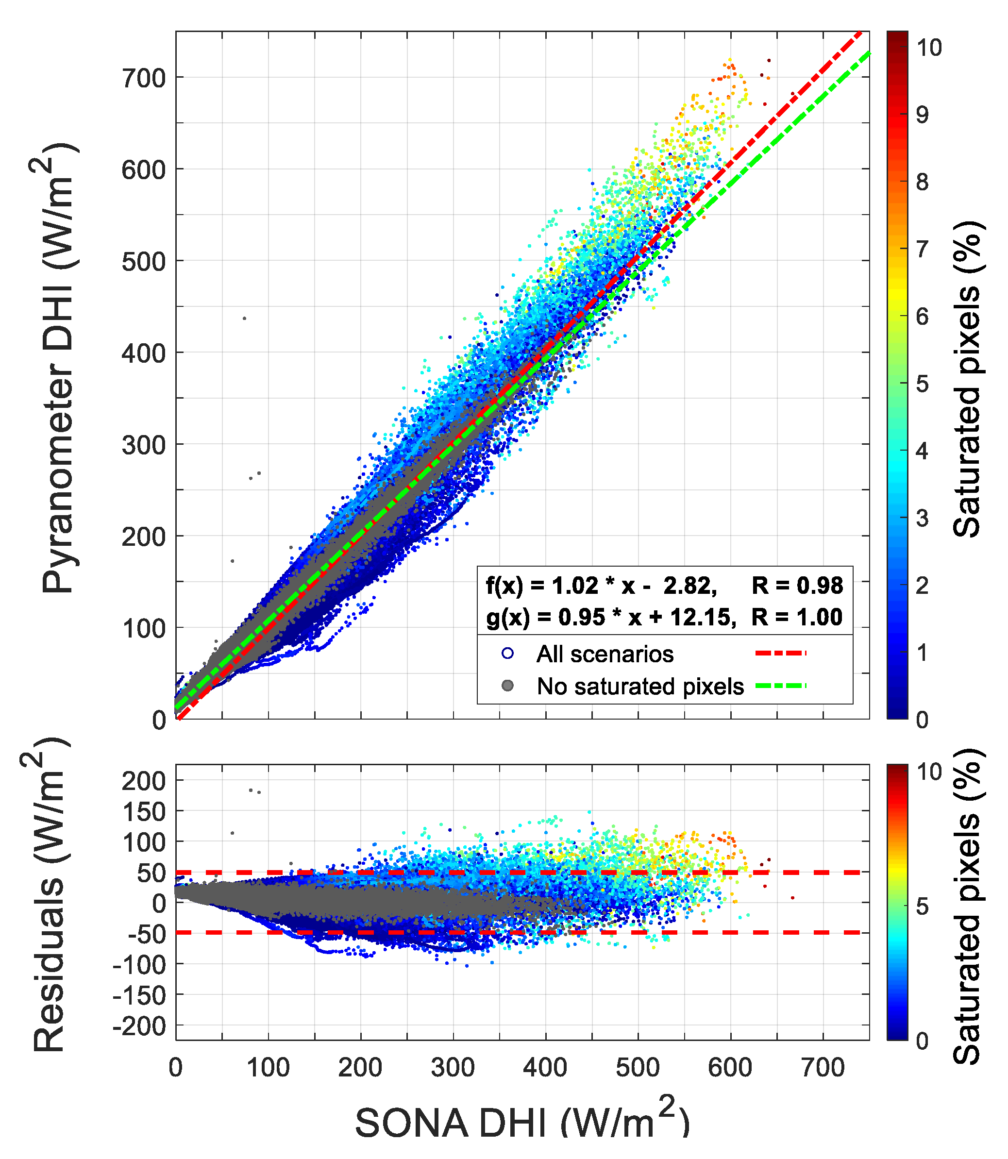
| Saturated Pixels for DHI Calculation | Sky Conditions | Slope | Offset | R | RMSE | N |
|---|---|---|---|---|---|---|
| Not considered | All | 2.10 | −20.60 | 0.98 | 21.40 | 287,398 |
| Considered as max Irradiance | All | 2.04 | −19.61 | 0.98 | 19.89 | 28,7398 |
| Not present | All | 1.97 | −7.28 | 1.00 | 6.84 | 86,108 |
Publisher’s Note: MDPI stays neutral with regard to jurisdictional claims in published maps and institutional affiliations. |
© 2021 by the authors. Licensee MDPI, Basel, Switzerland. This article is an open access article distributed under the terms and conditions of the Creative Commons Attribution (CC BY) license (https://creativecommons.org/licenses/by/4.0/).
Share and Cite
Valdelomar, P.C.; Gómez-Amo, J.L.; Peris-Ferrús, C.; Scarlatti, F.; Utrillas, M.P. Feasibility of Ground-Based Sky-Camera HDR Imagery to Determine Solar Irradiance and Sky Radiance over Different Geometries and Sky Conditions. Remote Sens. 2021, 13, 5157. https://doi.org/10.3390/rs13245157
Valdelomar PC, Gómez-Amo JL, Peris-Ferrús C, Scarlatti F, Utrillas MP. Feasibility of Ground-Based Sky-Camera HDR Imagery to Determine Solar Irradiance and Sky Radiance over Different Geometries and Sky Conditions. Remote Sensing. 2021; 13(24):5157. https://doi.org/10.3390/rs13245157
Chicago/Turabian StyleValdelomar, Pedro C., José L. Gómez-Amo, Caterina Peris-Ferrús, Francesco Scarlatti, and María Pilar Utrillas. 2021. "Feasibility of Ground-Based Sky-Camera HDR Imagery to Determine Solar Irradiance and Sky Radiance over Different Geometries and Sky Conditions" Remote Sensing 13, no. 24: 5157. https://doi.org/10.3390/rs13245157
APA StyleValdelomar, P. C., Gómez-Amo, J. L., Peris-Ferrús, C., Scarlatti, F., & Utrillas, M. P. (2021). Feasibility of Ground-Based Sky-Camera HDR Imagery to Determine Solar Irradiance and Sky Radiance over Different Geometries and Sky Conditions. Remote Sensing, 13(24), 5157. https://doi.org/10.3390/rs13245157