Article

An Efficient Lightweight Neural Network for Remote Sensing Image Change Detection

1
School of Instrumentation and Optoelectronic Engineering, Beihang University, Beijing 100191, China
2
Key Laboratory of Precision Opto-Mechatronics Technology, Ministry of Education, Beihang University, Beijing 100191, China
3
Beijing Advanced Innovation Center for Big Data-Based Precision Medicine, Beihang University, Beijing 100191, China
*
Author to whom correspondence should be addressed.
Remote Sens. 2021, 13(24), 5152; https://doi.org/10.3390/rs13245152
Submission received: 14 October 2021 / Revised: 13 December 2021 / Accepted: 16 December 2021 / Published: 18 December 2021
(This article belongs to the Special Issue 3D City Modelling and Change Detection Using Remote Sensing Data)

Abstract

:
Remote sensing (RS) image change detection (CD) is a critical technique of detecting land surface changes in earth observation. Deep learning (DL)-based approaches have gained popularity and have made remarkable progress in change detection. The recent advances in DL-based methods mainly focus on enhancing the feature representation ability for performance improvement. However, deeper networks incorporated with attention-based or multiscale context-based modules involve a large number of network parameters and require more inference time. In this paper, we first proposed an effective network called 3M-CDNet that requires about 3.12 M parameters for accuracy improvement. Furthermore, a lightweight variant called 1M-CDNet, which only requires about 1.26 M parameters, was proposed for computation efficiency with the limitation of computing power. 3M-CDNet and 1M-CDNet have the same backbone network architecture but different classifiers. Specifically, the application of deformable convolutions (DConv) in the lightweight backbone made the model gain a good geometric transformation modeling capacity for change detection. The two-level feature fusion strategy was applied to improve the feature representation. In addition, the classifier that has a plain design to facilitate the inference speed applied dropout regularization to improve generalization ability. Online data augmentation (DA) was also applied to alleviate overfitting during model training. Extensive experiments have been conducted on several public datasets for performance evaluation. Ablation studies have proved the effectiveness of the core components. Experiment results demonstrate that the proposed networks achieved performance improvements compared with the state-of-the-art methods. Specifically, 3M-CDNet achieved the best F1-score on two datasets, i.e., LEVIR-CD (0.9161) and Season-Varying (0.9749). Compared with existing methods, 1M-CDNet achieved a higher F1-score, i.e., LEVIR-CD (0.9118) and Season-Varying (0.9680). In addition, the runtime of 1M-CDNet is superior to most, which exhibits a better trade-off between accuracy and efficiency.

1. Introduction

With the ongoing increase in the world population and rapid urbanization processes, the global land surface has undergone significant changes. Therefore, the study of urbanization and environmental change interactions has drawn increased attention. With the breakthrough of earth observation techniques, massive remote sensing (RS) images provide a rich data source, such as satellite imagery, e.g., WorldView, QuickBird, GF2, and aerial images. In recent years, the spatial–spectral–temporal resolution of RS images has gradually improved. Nowadays, the availability of high- and very-high-resolution (VHR) images offers convenience for urban monitoring [1]. The remote sensing image interpretation techniques increasingly energize refined urban management. Specifically, change detection (CD) is one of the critical techniques. CD aims to identify and locate the change footprints based on multitemporal remote sensing images acquired over the same geographical region at different times [2]. Multitemporal RS images have the characteristics of macroscopicity and periodicity. CD has a wide range of applications, such as land cover and land use detection, urbanization monitoring, illegal construction identification, and damage assessment [3,4,5,6,7]. Furthermore, CD techniques can effectively reflect the development speed of the urbanization process. Specifically, the above-ground buildings are the most representative artificial structures. Therefore, building change detection can effectively reveal the development trend of urban spatial patterns. In this paper, the main concern was binary CD based on optical RS images. High-resolution optical images that reflect abundant spectral and spatial information of geospatial objects allow us to retain more details and obtain high-quality change maps. CD methods usually generate a pixel-level change map, in which pixels are classified as changed or unchanged. Many approaches have been explored to improve the accuracy and automation of change detection, which can be roughly divided into traditional [8] and deep learning (DL)-based methods [6].
According to the different analysis units for change detection, traditional change detection methods are roughly classified as the pixel-based method and object-based method [7,8]. In the early stage, change detection based on the RS images with low and medium spatial resolution is applied for land use and land cover change. Pixel-based methods were explored to obtain change information and reveal the ground surface change by using the spectral characteristics of pixels. The most representative methods are based on the difference images (DI), which is generated by image differencing, image ratio, or image transformation methods (such as change vector analysis (CVA) [9], principal component analysis (PCA) [4], and the regularized iteratively reweighted multivariate alteration detection (IR-MAD) method) [10]. DI indicates the magnitude of change. A change map can be generated based on the DI by the threshold method [11] and the clustering method [12]. Image transformation methods usually transform the RS images into a specific feature space, in which changed and unchanged pixels can be more discriminative using the extracted features. For instance, CVA is widely used to generate DI and obtain the change intensity. PCA is a typical method for feature dimension reduction. Celik proposed an unsupervised method based on PCA and k-means clustering method [13]. It applies PCA on the non-overlapping blocks of DI to extract feature vectors and utilizes the k-means algorithm to determine whether a corresponding pixel has changed. Due to the absence of context information, pixel-based methods are susceptible to noise, and, thus, the change detection results suffer from many pseudo-changes. Meanwhile, it is difficult to choose a property transformation method for a specific application scenario. With increased spatial resolution, pixel-based methods exhibit poor performance based on very-high-resolution (VHR) images [14].
High-resolution images can reflect the spatial distribution and geometric structure of geospatial objects. Alternatively, object-based methods effectively explore spatial information by employing the image object or superpixel as the basic processing unit [15,16,17]. Object-based methods have been widely studied, which utilize spectral, textural, and geometrical features for change detection. Object-based methods usually consist of three steps, i.e., object unit segmentation, object feature extraction, and feature classification [8]. Some machine learning methods are applied as classifiers for determining the change type, such as k-nearest neighbor (kNN) method [18], support vector machine (SVM) [19], random forest [20], and graphical models, i.e., Markov random field models [21] and conditional random field models (CRF) [14]. Besides, post-classification comparison methods [22] have been developed for specific tasks, which provide a complete matrix of change directions. Object-based methods are more suitable in high-resolution image change detection by measuring the similarity of segmented units. However, object-based methods are generally sensitive to segmentation errors. The detection accuracy highly depends on the results obtained by different segmentation strategies. To alleviate the problem, Lv et al. [14] combined the CRF method with the object-based technique to explore the spectral–spatial information. However, feature extraction and selection is a complex process that requires professional knowledge and experience, which limits the object-based methods’ application range. Traditional approaches based on hand-crafted features hinder their performance due to the limited representation of high-level semantics.
With the impressive breakthroughs in artificial intelligence and deep learning technology, CD methods have gradually evolved from traditional to DL-based approaches. Convolutional neural network (CNN) has an inherent advantage of feature representation. Thus, CNN becomes a better solution for feature extraction than hand-crafted features [23]. In recent years, CNN-based methods have made remarkable progress in remote sensing image change detection [6]. Specifically, the supervised methods based on prior knowledge provided from manually annotated labels achieve better performance than traditional methods in terms of accuracy and robustness. Some attempts were inspired by the image semantic segmentation models, such as UNet [24] and UNet++ [25]. The proposed change detection networks are based on a U-shape encoder–decoder architecture [26,27,28,29]. These methods emphasize end-to-end change detection, which is implemented by constructing a fully convolutional network. Different from the image segmentation tasks, change detection involves a pair of bi-temporal images as an input of the model.
The network framework can be roughly divided into early- and late-fusion frameworks [30]. The early-fusion framework concatenates the bi-temporal images along the channel axis as an input of the network. The late-fusion framework extracts feature maps from the two co-registered images using a parallel dual-stream network separately, where two branches usually share the same structure. If the two branches share weights, it is the so-called Siamese framework; otherwise, it is the pseudo-Siamese framework [26]. Daudt et al. implemented end-to-end change detection based on the pseudo-Siamese framework, i.e., fully convolutional Siamese-difference network (FC-Siam-diff) and fully convolutional Siamese-concatenation network (FC-Siam-conc) [26]. The difference lies in how the skip connections are performed. The former concatenates the absolute value of bi-temporal features’ difference during the decoding phase. The latter directly concatenates the bi-temporal features instead. Hou et al. [31] extended UNet and proposed a Siamese variant called W-Net for building change detection. W-Net learns the difference features of bi-temporal features by comparison in the feature domain. Though attractive in improving accuracy by fusing features through skip connections, checkerboard artifacts caused by deconvolutions during decoding becomes one of the main concerns. Alternatively, upsampling combined with convolutions is a good solution to alleviate checkerboard artifacts of the detection results. For instance, Zhang et al. [30] proposed a deeply supervised image fusion network (IFN) based on the pseudo-Siamese framework. More precisely, they introduced the CBAM attention modules [32] during decoding for overcoming the heterogeneity problem. Similarly, Fang et al. [33] proposed the SNUNet-CD based on the Siamese network and UNet++. The ensemble channel attention module (ECAM) was applied for aggregating and refining features of multiple semantic levels. Wang et al. [28] proposed a pseudo-Siamese network called ADS-Net that emphasizes feature fusion using a mid-layer fusion method. Instead, Zhang et al. [34] proposed a hierarchical network, called HDFNet, which introduces dynamic convolution modules into decoding stages for emphasizing feature fusion. The aforementioned works share a similarity in that skip connections are applied to concatenate deep features with low-level features during the decoding stage for performance improvement. These studies demonstrated that both high-level semantic information and low-level detail information are important in change detection. Unfortunately, which feature fusion strategy is the better is not clear. Dense skip connections bring about high computational costs.
Alternatively, Daudt et al. [35] proposed FC-EF-Res that adopts the early-fusion framework based on UNet by incorporating residual modules [36]. FC-EF-Res utilizes the residual modules to facilitate the training of the deeper network. FC-EF-Res achieved better performance than FC-Siam-diff and FC-Siam-conc. Zheng et al. [29] proposed a lightweight model CLNet based on the U-Net, which builds the encoder part by incorporating the cross-layer blocks (CLBs). An input feature map was first divided into two parallel but asymmetric branches. Then, CLBs apply convolution kernels with different strides to capture multi-scale context for performance improvement. More recently, some attempts that adopt early-fusion frameworks were developed based on the UNet++. Peng et al. [27] proposed an improved UNet++ with multiple side-outputs fusion (MSOF) for change detection in high-resolution images. The dense skip structure of UNet++ facilitates multilayer feature fusion. Peng et al. [37] proposed a simplified UNet++ called DDCNN that utilizes dense upsampling attention units for accuracy improvement. Zhang et al. [38] proposed DifUnet++, which emphasizes the explicit representation of difference features using a differential pyramid of bi-temporal images. Yu et al. [39] implemented the NestNet based on the UNet++. NestNet promotes the explicit difference representation using absolute differential operation (ADO). During model training, multistage prediction and deep supervision have been proven effective strategies for achieving better performance. For instance, some attempts apply the multistage prediction strategy at the decoder’s output side, such as Peng et al. [27], DifUnet++ [38], NestNet [39], IFN [30], HDFNet [34], and ADS-Net [28]. The overall loss function is calculated based on the weighted sum of multistage prediction’s loss. The deep supervision strategy facilitates the network convergence during the training phase, whereas it brings about more computation and memory cost than single-head prediction. Besides, high-level features have a coarse resolution but are accurate in semantic representation compared with low-level features. However, low-level features are more accurate in spatial location. ADS-Net [28] and IFN [30] methods employed the spatial–channel attention modules for feature fusion during decoding. Peng et al. [37] proposed the upsampling attention unit for promoting feature fusion during upsampling. High-level features are applied to guide the selection of low-level features for performance improvement.
Recently, change detection methods by incorporating attention mechanisms [40] have drawn considerable attention. Attention mechanisms have been widely studied in computer vision, such as the self-attention model (e.g., Non-local [41]), the channel attention model (e.g., squeeze and excitation modules [42]), and spatial–channel attention model (e.g., CBAM [32] and DANet [43]). Some attempts introduce attention modules in the network, which learns discriminative features and alleviates distractions caused by pseudo-changes. For example, Chen et al. [44] proposed STANet that consists of a feature extraction network and a pyramid spatial–temporal attention module (PAM). ResNet-18 was applied for feature extraction, and the self-attention module was used to calculate the attention weights and model the spatial–temporal relationships at various scales. STANet with PAM achieved a better F1-score than the baseline. When training with sufficient samples, attention-based methods achieve superior performance in accuracy and robustness. More recently, transformer-based models have achieved a breakthrough in computer vision field, such as ViT [45] for image classification, DETR [46] for object detection, and SETR [47] for image semantic segmentation. Chen et al. [48] proposed BIT_CD that combines the transformer with CNN to solve the bitemporal image change detection. BIT_CD adopts a transformer encoder to model contexts in the compact semantic token-based space-time. BIT_CD outperforms some attention-based methods, such as STANet [44] and IFN [30].
We can conclude that the recent advances in DL-based CD methods mainly focus on improving precision through enhancing the feature representation ability of the model. Some attempts employed deeper networks to address the issue. These methods applied multilevel feature extraction and fusion for multiscale context modeling. Thus, though attractive in improving performance by applying a deep supervision strategy for model training, the model consumes massive memory cost. More recent attempts introduced attention modules for promoting the discrimination of features. Based on the supervised technique, these methods achieve state-of-the-art interpretation accuracy. However, the increase in the network depth and width that involves a large number of network parameters requires large memory space for storage. In addition, the deeper networks incorporated with attention-based or multiscale context-based modules usually consume massive memory during training and require more inference time. It hinders the interpretation efficiency of massive remote sensing images in practice. Recently, some lightweight change detection networks have been proposed. Chen et al. [49] proposed a lightweight multiscale spatial pooling network to exploit the spatial context information on changed regions for bitemporal SAR image change detection. Wang et al. [50] proposed a lightweight network that replaces normal convolutional layers with bottleneck layers and employs dilated convolutional kernels with a few non-zero entries that reduce the running time in convolutional operators. However, they did not give a specific number of network parameters and computations. It is hard to evaluate the computational efficiency in practice. In this sense, a lightweight network is designed to promote the inference speed and achieve high computational efficiency. We attempt to design an efficient network that achieves accuracy improvements and comparable inference speed.
The main contributions of this paper are summarized as follows. This paper first proposed an effective network, called 3M-CDNet, for accuracy improvement. It requires about 3.12 M trainable parameters. The network consists of a lightweight backbone network and a concise classifier. The former is used for feature extraction, and the latter is used to classify the extracted features and generate a change probability map. Moreover, a lightweight variant called 1M-CDNet that only requires about 1.26 M parameters was proposed for computation efficiency with the limitation of computing power. 3M-CDNet and 1M-CDNet have the same backbone network architecture but different classifiers. The lightweight network incorporates deformable convolutions (DConv) [51,52] into the residual blocks to enhance the geometric transformation modeling ability for change detection. Besides, change detection was implemented based on high-resolution feature maps to promote the detection of small changed geospatial objects. A two-level feature fusion strategy was applied to improve the feature representation. Dropout [53] was applied in the classifier to improve the generalization ability. The networks achieved better accuracy compared with the state-of-the-art methods while reducing network parameters. Specifically, the inference runtime of the proposed 1M-CDNet is superior to most existing methods.
The rest of this paper is organized as follows. Section 2 presents the method proposed in this paper, including the DConv-based backbone network in Section 2.1 and the pixel-wise classifier in Section 2.2. Section 3 discusses the experimental results on public datasets, including method comparison in Section 3.5.1 and Section 3.5.2. Section 4 discusses the ablation studies. Conclusions are shared in Section 5.

2. Proposed Method

In this section, we present the proposed effective network for urban change detection in remote sensing images. The proposed 3M-CDNet only involves about 3.12 M trainable parameters. As shown in Figure 1, 3M-CDNet mainly consists of two core components: Figure 1a shows a deformable convolution (DConv)-based backbone network, and Figure 1b shows a pixel-wise classifier. The former is used for feature extraction from the input I 1 , 2 6 × H × W The latter is used to classify the extracted features into two classes in a change probability map. The network adopts the early-fusion framework and takes as an input with six bands a pair of bitemporal RGB images. Then, it generates a binary change map C M 1 × H × W , where pixels are either changed or unchanged. 3M-CDNet has a modular structure with high flexibility. It allows achieving performance improvement by incorporating some plug-and-play modules, such as DConv [52] and dropout regularization [53]. In addition, a lightweight variant, called 1M-CDNet, was proposed to reduce computation costs for computation efficiency by using a simpler classifier with fewer trainable parameters.
First, we introduced the network architecture, i.e., the DConv-based backbone network and the pixel-wise classifier. Second, the loss function definition for model training was described.

2.1. DConv-Based Backbone Network

As shown in Figure 1a, the backbone network of 3M-CDNet is composed of the Input Layer, Layer 1, and Layer 2. The main concern is to reduce the size of input through consecutive downsampling and convolution operations, and extract features maps with varying degrees of semantics from shallow to deep layers. Specifically, the Input Layer consists of three stacked 3 × 3 convolutional layers followed by a MaxPool layer. The Input Layer is applied to downsample the input and transform I 1 , 2 6 × H × W into a 3-D tensor X 0 128 × H 4 × W 4 . The spatial resolution is 1/4 of the input size. X 1 s t 256 × H 4 × W 4 and X 2 n d 512 × H 4 × W 4 are feature maps extracted from Layer 1 and Layer 2, respectively.

2.1.1. Introducing Residual Network

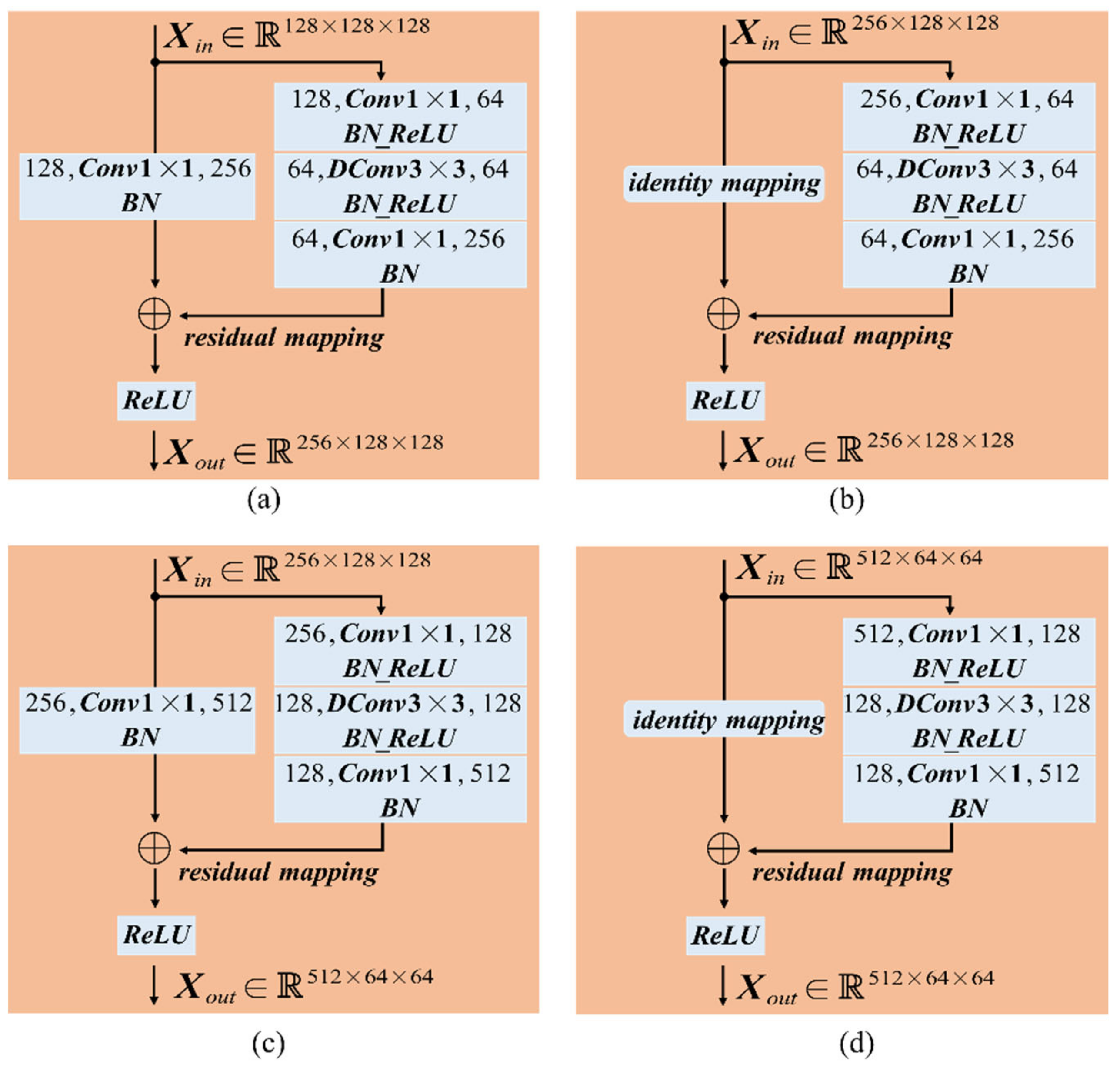
When the CNN goes deeper, which could hamper the convergence, it leads to a degradation problem [36]. Therefore, Layer 1 and Layer 2 were designed based on the residual network [36]. Bottleneck residual blocks were designed as basic units of Layer 1 and Layer 2, which have the advantage of alleviating the degradation problem and promoting convergence during training. As shown in Figure 2c, bottleneck blocks can be formulated as follows:
X o u t l = R e L U H X i n l + ξ X i n l ,   Ω l ,
where X i n l and X o u t l are the input and output tensors of the lth residual block, respectively. ξ · indicates the residual mapping function, i.e., the right branch that consists of three stacked convolution layers. Specifically, the Conv1 × 1, Conv3 × 3, and Conv1 × 1 are applied in series to model the residual mapping function ξ · . The number of feature channels is first reduced and then increased, also known as the bottleneck structure. H · indicates the identity mapping function, i.e., the left branch. H · applies a downsampling projection shortcut through a Conv1 × 1 and a batch normalization (BN) layer only if stride is set to 2, e.g., the first block of Layer 2. Otherwise, an identity shortcut is identified. Besides, BN is also applied at the tail end of each convolution kernel to facilitate the training procedure more stable. The results of ξ · and H · are further merged by element-wise summation. R e L U · is the rectified linear unit activation function for enhancing the non-linear fitting ability. R e L U · can be expressed in f z = max 0 ,   z .
The detailed architecture of the backbone network is described in Table 1. For instance, the size of input images is set to 6 × 512 × 512. Layer1_x indicates that Layer1 is composed of three residual blocks in series, i.e., Layer1_1, Layer1_2, and Layer1_3. The stride of all filters is set to 1. Layer1_1 adopts the structure as shown in Figure 2a. Layer1_2 and Layer1_3 adopt the structure as shown in Figure 2b. Layer2_x indicates that Layer2 is composed of four residual blocks in series, i.e., Layer2_1, Layer2_2, Layer2_3, and Layer2_4. Layer2_1 adopts the structure as shown in Figure 2c. Layer2_1 applies downsampling on the output feature maps of Layer1_3 and reduces the size of feature maps to half. Therefore, the stride of the Conv1 × 1 in H · and Conv3 × 3 in ξ · is set to 2, while the stride of the Conv1 × 1 in ξ · is set to 1. The remained three blocks adopt the structure as shown in Figure 2d. The stride of their filters is set to 1. Besides, a bilinear upsample layer Layer2_Upsample_2× upsamples the extracted features to the 1/4 size of the input.
Therefore, change detection is implemented based on high-resolution feature maps. Unlike the original ResNet [36], which has too many downsampling operations, spatial details in deep features are lost, and high-resolution features promote the detection of small changed objects. We reduced the width and depth of the backbone network so that the number of parameters decreased. However, the receptive field of deep features is limited due to the limitation of the backbone network’s depth. It is difficult to keep the completeness of the contextual semantics in deep features. The limited receptive field leads to weak feature representation [54]. To alleviate the problem, deformable convolutions [51,52] provide a feasible solution. We introduced deformable convolutions in residual blocks for capturing deformable context from objects with various shapes and scales.

2.1.2. Introducing Deformable Convolutions

Let X i n p and X o u t p denote the feature at location p of the input and output feature maps, respectively. Given a convolution kernel of K sampling locations, let w k and p k denote the weight value and default offset for the kth location of the kernel, respectively, e.g., a 3 × 3 kernel with p k 1 , 1 , 1 ,   0 , , 1 ,   1 | K = 9 . Two-dimensional convolutions sample the input feature map with a fixed grid can be formulated as follows:
X o u t p = k = 1 K w k · X i n p + p k ,
where w k enumerates the weights of the kernel according to the kth location.
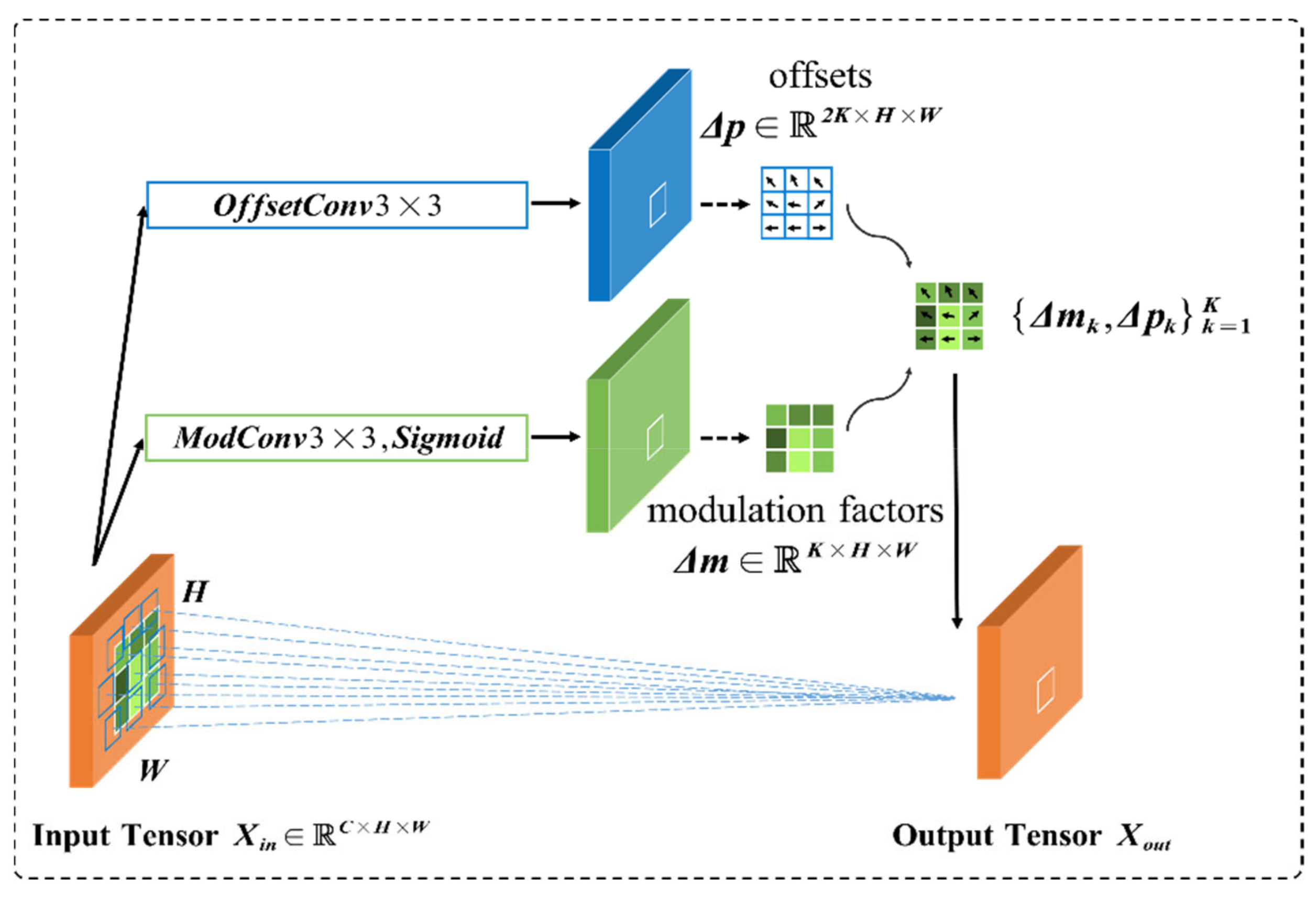
Convolutions that sample the input feature map using a fixed and regular grid have a fixed receptive field. We introduced deformable convolutions (DConv) [52] to promote the ability of modeling geometric transformation. DConv achieves arbitrary deformation of the receptive field by adjusting the 2-D offsets and modulation factors of sampling locations. Deformable contexts adaptively build long-range dependencies based on the structural information of geospatial objects. DConv can be formulated as follows:
X o u t p = k = 1 K w k · X i n p + p k + Δ p k · Δ m k ,
where Δ p k and Δ m k are the learnable 2-D offsets and modulation factor for the kth location, respectively. Δ p k includes the x and y directions’ offsets.
As shown in Figure 3, let X i n C × H × W denote the input feature map of DConv3 × 3, and p i denote the center location of the kernel. Two convolution layers, O f f s e t C o n v 3 × 3 and M o d C o n v 3 × 3 , are separately applied over the input feature maps to obtain Δ p k and Δ m k . The number of filters is set to 2K for O f f s e t C o n v 3 × 3 and K for M o d C o n v 3 × 3 . The former generates the feature map of the learned 2-D offsets, i.e., Δ p = Δ p k i k = 1 K = Δ x k i ,   Δ y k i k = 1 K 2 K × H × W ,   1 i H · W ,   K = 9 . The latter followed by a Sigmoid activation function generates the feature map of modulation factors, i.e., Δ m = Δ m k i k = 1 K K × H × W ,   1 i H · W ,   K = 9 . The Sigmoid function transforms modulation factors to the range (0, 1), which is expressed in f z = 1 1 + exp z .
Due to the fractional coordinate p + p k + Δ p k , the value of X i n p + p k + Δ p k is calculated based on the values of the four surrounding integer points by bilinear interpolation. In summary, DConv consists of two key steps. First, it generates deformable feature maps from the input feature maps based on the learned offsets in the x and y directions Δ p k = Δ x k , Δ y k k = 1 K and applies the learned modulation factors Δ m k k = 1 K 0 ,   1 to modulate the activation of each location. Next, it applies a regular 2-D convolution over the deformable feature maps and then generates the output feature maps. In this paper, DConvs are applied to replace all the 3 × 3 convolution layers of the bottleneck blocks, termed DConvBottleneck. In this way, the DConv-based backbone network is enforced to adaptively generate a more explicit spatial feature representation. Therefore, 3M-CDNet has the advantage of overcoming the adverse effects of scale variations of objects with various shapes.

2.1.3. Multilevel Feature Fusion Strategies

Previous works demonstrate that both high-level semantics and low-level detail information are important in change detection. Based on the DConv-based backbone network, a two-level strategy is applied to improve the feature representation by fusing the features X 2 n d and X 1 s t . The channel concatenation operation was selected for its simplicity to achieve high computational efficiency using the minimal number of parameters.
It is rare for previous studies to clearly state which feature fusion strategy is effective. We compare three kinds of feature fusion strategies, which are as follows: (1) only applying the high-level feature maps X 2 n d , termed the one-level strategy; (2) applying the fusion feature maps X obtained by concatenating the high-level X 2 n d and low-level X 1 s t along the channel axis, i.e., X = X 1 s t X 2 n d , termed the two-level strategy; and (3) applying the two-level strategy and then an extra fusion feature map X ^ 384 × H 4 × W 4 , which is obtained by concatenating the output feature maps of the first 1 × 1 convolution layer of the classifier and X θ extracted by the Input Layer, termed the three-level strategy.

2.2. Pixelwise Classifier

The pixel-wise classifier of 3M-CDNet adopts a plain design that only consists of four convolution layers in series. Table 2 presents the detailed architecture of the 3M-CDNet classifier. First, a 1 × 1 convolution layer Conv3_1 transforms the fusion features and reduces the feature channels from 768-D to 256-D. To obtain a change map of the same spatial resolution as the input, a 2-fold bilinear upsampling is applied after the first and last 1 × 1 convolution layers. The subsequent convolution layers classify the extracted features into two classes and predict a change probability map C M p r o b 1 × H × W through a sigmoid layer, of which the values lie in the range (0, 1). Finally, the binary change map C M 1 × H × W can be generated by applying thresholding over C M p r o b 1 × H × W with a fixed threshold.
As shown in Table 2, change detection was implemented based on a high-resolution feature map, i.e., the input feature map of Conv3_2, to promote the detection of small changed geospatial objects. Therefore, the two Conv3 × 3 (Conv3_2 & Conv3_3) with a large number of input/output channels have high computation costs, which occupy about 80% computation of 3M-CDNet. For example, when the size of bi-temporal input images is set to 6 × 512 × 512, the two Conv3 × 3 (Conv3_2 & Conv3_3) take as input a high-resolution feature map with a shape of 256 × 256 × 256, i.e., X 256 × H 2 × W 2 . The resolution of the internal feature is half of the input images. The computation costs of a convolution operator can be formulated as follows:
FLOPs = K h × K w × C i n × C o u t × H o u t × W o u t
where K h = 3 ,   K w = 3 denote the kernel size; C i n = 256 ,   C o u t = 256 denote the input/output channels; and H o u t = 256 ,     W o u t = 256 denote the size of output internal feature map. We can observe that the computation of one Conv3 × 3 is about 38.65 GFLOPs, and that of two Conv3 × 3 is about 77.31 GFLOPs in total.
Due to the limitation of computing power in some practical platforms, a lightweight variant called 1M-CDNet was proposed to reduce computation costs for computation efficiency by using a simpler classifier with fewer trainable parameters. Compared with 3M-CDNet, 1M-CDNet’s classifier only has three 1 × 1 convolution layers to facilitate the inference speed, as shown in Table 3. The computation costs (4.34 GFLOPs) will be sharply reduced compared with that of 3M-CDNet’s classifier (80.66 GFLOPs) when the size of bi-temporal input images is set to 6 × 512 × 512. The proposed networks allow us to flexibly adjust the classifier to match different application requirements and limitations in practice.

2.2.1. Introducing Dropout Regularization

Dropout [53] is a simple yet effective way to prevent neural networks from overfitting. During training, dropout randomly drops units from the network with a certain probability p d , which can be equivalent to training numerous different networks simultaneously, i.e., D X = D m X , where D m indicates a binary mask of the same size with the feature map X , and indicates the element-wise multiplication operation. D m is randomly generated from a Bernoulli distribution with a probability p d , and the units of the feature maps corresponding to the locations of zeros are to be discarded during training. At test time, a neural unit is always presented, and the weights are multiplied by p d so that the output of the unit would be the same as the expected output at training time, i.e., D X = p d X . In this paper, two dropout layers with probabilities of 0.5 and 0.1 are applied at the tail end of the classifier’s 3 × 3 convolution layers.

2.2.2. Binarization

The trained model outputs the change probability activation map, i.e., C M p r o b 1 × H × W . A fixed threshold segmentation method is applied on C M p r o b 1 × H × W for binarization. It generates a binary change map with the same size as the input image, i.e., C M 1 × H × W . It can be formulated as shown in Equation (5).
C M i , j = 1 ,     i f   C M p r o b i , j > T 0 ,     o t h e r w i s e ,
The subscript i , j 1 i H , 1 j W indicates the indexes of the change map’s height and width, respectively. T indicates a fixed binarization threshold to determine whether a pixel has changed. A pixel is classified as changed if and only if the change probability is larger than T; otherwise, it is classified as background. In this paper, T was empirically set to 0.5 for simplicity.

2.3. Loss Function Definition

During training, network parameters are iteratively updated by minimizing the loss between the forward output of 3M-CDNet and the reference change map with the backpropagation (BP) algorithm according to a specific loss function. The similarity between two probability distributions can be measured by counting the cross-entropy loss. Change detection aims to classify all the pixels into two subsets, i.e., changed and unchanged. The binary cross-entropy (BCE) loss function becomes an intuitive candidate for model training, which can be formulated as shown in Equation (6).
L b c e = 1 N n = 1 N y n log y ^ n + 1 y n log 1 y ^ n ,
The parameter N is the number of samples. Each pixel is counted as a sample. The parameter y n indicates an unchanged or changed pixel of the reference change map, and y ^ n 0 , 1 denotes the prediction of the model.
However, the number of unchanged pixels is usually more than that of changed pixels. Due to the widespread class imbalance, dominant unchanged pixels would make models tend to collapse and increase the difficulty during training. To alleviate this issue, the soft Jaccard index is introduced. The loss function can be formulated as shown in Equation (7).
L b c d = λ 1 N n = 1 N y n log y ^ n + 1 y n log 1 y ^ n + 1 λ 1 N log n = 1 N y n y ^ n y n + y ^ n y n y ^ n ,
The parameter λ 0 , 1 is the weight factor to balance the BCE loss and Jaccard loss. In this paper, λ was empirically set to 0.7.

3. Experiments and Results

3.1. Experimental Dataset

For model training and evaluation, we adopted two representative datasets, including LEVIR-CD [44] and Season-Varying [55]. We then applied the criteria as recommended by the creators to split the datasets. We trained the model for 300 epochs and 600 epochs on two datasets, respectively.
(1) LEVIR-CD Dataset (https://justchenhao.github.io/LEVIR/, accessed on 6 July 2021). The dataset contains 637 pairs of co-registered very-high-resolution (VHR, 0.5 m/pixel) Google Earth images with a size of 1024 × 1024 pixels. These bitemporal images with a period of 5∼14 years were collected from 20 different regions that sit in several cities in Texas of the US. This dataset mainly focuses on building-related changes, including the building growth (the change from soil/grass/hardened ground or building under construction to new build-up regions) and the building decline. The buildings have various types and scales. Besides, irrelevant changes caused by seasonal changes and illumination changes bring about challenges. The number of changed and unchanged pixels is 30,913,975 and 637,028,937, respectively. The creator randomly split the dataset into three parts, i.e., 70% samples for training, 10% for validation, and 20% for testing [44]. Due to the limitation of GPU memory, the original images were cropped into smaller image tiles with a size of 512 × 512 pixels for model training and evaluation. In our case, 4016 and 1024 tiles were cropped for training and validation using a sliding window with a stride of 256 overlapping pixels, respectively. In addition, 512 non-overlapping tiles were cropped for testing.
(2) Season-Varying Dataset (https://drive.google.com/file/d/1GX656JqqOyBi_Ef0w65kDGVto-nHrNs9, accessed on 6 July 2021). The dataset contains 7 pairs of co-registered images with the size of 4725 × 2700 pixels for manual ground truth creation, which were obtained by Google Earth (DigitalGlobe). Bitemporal images with seasonal changes were introduced in this dataset, such as from summer to winter/autumn. The spatial resolution of these images is from 3 to 100 cm/pixel. The change types are mainly related to land changes, building changes, road changes, and car changes. Each pair of images was cropped into randomly rotated fragments (0–2π) with a size of 256 × 256 pixels and at least a fraction of changed pixels. Finally, Season-Varying contains 16,000 pairs of image tiles with fixed size 256 × 256 pixels, of which 10,000 and 3000 tiles are used for training and validation, respectively, and an extra 3000 tiles were used for testing [55].
Specially, we used each pair of images in the dataset to get the PSNR of each bi-temporal images, and then averaged them to get the PSNR of the datasets. PSNR for LEVIR-CD and Season-Varying is approximately 13 dB and 11 dB, respectively.

3.2. Evaluation Metrics

The most common metrics related to the changed category were adopted for the quantitative evaluation, including overall accuracy (OA), precision (Pr), recall (Re), F1-score (F1) (https://nndl.github.io/nndl-book.pdf, accessed on 16 November 2021), and the intersection of union (IoU) [24]. The above metrics related to the changed category can be formulated as follows.
P r = T P T P + F P
    R e = T P T P + F N
F 1 = 2 × P r × R e P r + R e
I o U = T P T P + F P + F N
O A = T P + T N T P + F P + T N + F N
In binary change detection, true positive (TP) indicates the number of pixels misclassified as changed. False positive (FP) indicates the number of pixels correctly classified as changed. False negative (FN) indicates the number of pixels misclassified as unchanged. True negative (TN) indicates the number of correctly classified as unchanged. Pr indicates the ratio of the number of correctly classified positive samples to that of samples classified as positive by the classifier. Re indicates the ratio of the number of correctly classified positive samples to that of all positive samples. F1 is a harmonic mean of Pr and Re. F1 and IoU are comprehensive indicators to reveal the overall performance; the higher the value, the better the performance.
Besides, the time complexity of the models is measured by the runtime and computational costs. Specifically, runtime (ms) is measured by counting the average time of randomly running a forward prediction 1000 times during the testing phase. Computational costs are measured by counting the number of floating-point operations (FLOPs) [48] in the testing phase, i.e., 1 GFLOPs = 1 × 10⁹ FLOPs.

3.3. Experiment Settings

3.3.1. Implementation Details

The proposed 1M-CDNet and 3M-CDNet were implemented in Python using PyTorch framework [56]. During training, the AdamW optimizer [57] is used for updating the network parameters. The AdamW optimizer has the advantage of adapting its parameter-wise learning rates and facilitating convergence. AdamW means Adam with decoupled weight decay. The decoupled weight decay renders the optimal settings of the learning rate and the weight decay factor more independent, thereby simplifying the hyperparameter optimization. It allows us to apply AdamW for model training using a fixed learning rate schedule and weight decay, which reduces the difficulty of hyperparameter choice. During the training phase, the model was optimized by minimizing Equation (6) through the AdamW optimizer with β 1 = 0.9 and β 2 = 0.99 , of which the initial learning rate and weight decay were empirically set to 0.000125 and 0.0005, respectively. The minibatch size was set to 16 on an NVIDIA RTX 3090 GPU with 24 GB memory. The operating system is Ubuntu 18.04 with 128 GB memory, and the CPU is Intel(R) Xeon(R) Silver 4215R.

3.3.2. Online Data Augmentation

Data augmentation (DA) is a simple yet effective technique for regularizing the network. DA can be used to simulate scale variations, illumination variations, and pseudo-changes, such as the spectra changes between bitemporal images. Online data augmentation means that DA is only performed when training instead of expanding the original training set at the cost of expensive training time. In this paper, online data augmentation was randomly applied after every batch data loaded, with a probability of 0.8 by randomly shifting-rotating-scaling with padding zeros, rotating by 90°, 180°, and 270°, and flipping in horizontal and vertical directions, and applying color jitter. Each kind of augmentation was randomly applied with a probability of 0.5. Online DA is equivalent to an implicit expansion of the training data set, which can increase the randomness of the training while avoiding the linear level of the original training data set.

3.4. Comparative Methods

Several state-of-the-art deep learning-based CD methods were selected for comparison purposes. These methods were introduced in brief, including four pure fully convolutional network (FCN)-based methods (FC-Siam-Diff [26], FC-Siam-Conc [26], FC-EF-Res [35], and CLNet [29]), three attention-based methods (STANet [44], DDCNN [37], and FarSeg [58]), a transformer-based BIT-CD [48], and two light-weight networks (MSPP-Net [49] and Lite-CNN [50]). Specifically, the authors of STANet and BIT-CD are exactly the creators of LEVIR-CD dataset.
(1)
FC-Siam-Diff [26]. A feature-level late-fusion method, which uses a pseudo-Siamese FCN to extract and fuse the bitemporal multilevel features by a feature difference operation.
(2)
FC-Siam-Conc [26]. It is very similar to FC-Siam-Diff. The difference lies in the way to fuse the bitemporal features by a feature concatenation operation.
(3)
FC-EF-Res [35]. An image-level early-fusion method. The network takes as an input the concatenated bitemporal images. It introduced the residual modules to facilitate network convergence easily.
(4)
CLNet [29]. A U-Net based early-fusion method, which builds the encoder part by incorporating the cross layer blocks (CLBs). An input feature map was first divided into two parallel but asymmetric branches, then CLBs apply convolution kernels with different strides to capture multi-scale context for performance improvement.
(5)
STANet [44]. A metric-based method, which adopts a Siamese FCN for feature extraction and learns the change map based on the distances between the bitemporal features. Inspired by the self-attention mechanism, a spatial–temporal attention module was proposed to learn the spatial–temporal relationships between the bitemporal images to generate more discriminative features.
(6)
DDCNN [37]. An attention-based method that adopts a simplified UNet++ architecture. Combined with the dense upsampling units, high-level features were applied to guide the selection of low-level features during the upsampling phase for performance improvement.
(7)
FarSeg [56]. A foreground-aware relation network for geospatial objects segmentation in RS images. From the perspective of relation, FarSeg enhances the discrimination of foreground features via foreground-correlated contexts associated by learning foreground scene relation.
(8)
BIT-CD [48]. A transformer-based method, which expresses the input images into a few high-level semantic tokens. By incorporating a transformer encoder in the CNN backbone network, BIT-CD models the context in a compact token-based space-time.
(9)
MSPP-Net [49]. A lightweight multi-scale spatial pooling (MSPP) network was used to exploit the changed information from the noisy difference image. Multi-scale pooling kernels are equipped in a convolutional network to exploit the spatial context information on changed regions from images.
(10)
Lite-CNN [50]. A lightweight network replaces normal convolutional layers with bottleneck layers that keep the same number of channels between input and output. It also employs dilated convolutional kernels with a few non-zero entries that reduce the running time in convolutional operators.
Table 4 presents the number of parameters (M), the computational costs (GFLOPs), and the inference runtime (ms) of different CD networks. All results presented in Table 4 were measured on an NVIDIA RTX 2080Ti GPU with 11-GB memory. When calculating the computational cost during testing, it takes 6 × 256 × 256 and 6 × 512 × 512 fixed-size as inputs. The runtime was measured with different batch sizes (“bs”) during testing, where “bs” was set 1 and 16, respectively. Note that DDCNN and STANet that consume massive memory cost cannot run on a single GPU with 11-GB memory under the setting with “bs = 16”, where an error called CUDA out of memory occurred.
In light of using high-resolution features for change detection, 3M-CDNet costs 23.71 G and 94.83 GFLOPs, and 1M-CDNet costs 4.54 G and 18.14 GFLOPs, according to the input size of 6 × 256 × 256 and 6 × 512 × 512 . We can observe that the inference speed of 1M-CDNet is superior to most existing methods under the setting with “bs = 16” and “bs = 1”. From Table 4, we can observe that 1M-CDNet only involves 1.26 M parameters, which are about 3% of FarSeg that requires 31.38 M. Specifically, 1M-CDNet requires much fewer parameters than DDCNN and reduces the computational costs. Table 4 shows the number of parameters of DDCNN (60.21 M) is about 47 times that of 1M-CDNet, and DDCNN’s computational cost (214.16 GFLOPs) is about 46 times of 1M-CDNet. What is more, compared with the lightweight model, such as CLNet, BIT-CD, FC-Siam-Diff, and FC-Siam-Conc, 1M-CDNet achieves better accuracy with comparable runtime. More details of the experimental results will be discussed in Section 3.5.

3.5. Experiment Results

3.5.1. Comparisons on LEVIR-CD Dataset

(a) 
Quantitative evaluation
Table 5 presents the quantitative results on the LEVIR-CD dataset. Due to the effectiveness of aggregating multiscale context, we can observe that CLNet and DDCNN achieve remarkable progress with a significant margin compared with the pure FCN-based FC-Siam-Conc, FC-Siam-Diff, and FC-EF-Res. Instead, our 1M-CDNet and 3M-CDNet do not apply sophisticated structures, such as UNet++ or UNet with dense skip connections as well as the deep supervision strategy for facilitating intermedia layers, which are powerful for pixel-wise prediction tasks. Nonetheless, the quantitative results show that 1M-CDNet and 3M-CDNet consistently outperform the other approaches in terms of the comprehensive metrics F1 and IoU. 3M-CDNet achieves the best F1 (0.9161) and IoU (0.8452), which perform better than the baseline STANet with a significant improvement of F1 (+3.53%) and IoU (+5.83%). Besides, 1M-CDNet achieves the second best F1 (0.9118) and IoU (0.8379). Table 5 suggests that 1M-CDNet outperforms the state-of-the-art CLNet (w/DA), which increased by about IoU (+0.82%) and F1 (+0.49%), respectively, with fewer computation costs. Moreover, as for Pr and Re metrics, Table 5 suggests that DDCNN achieves the highest Pr, but its Re is low, indicating that DDCNN detects fewer change areas. STANet achieves the highest Re, but its Pr is low, indicating that STANet detects more errors in the changing area. 3M-CDNet makes a better trade-off between precision (91.99%) and recall (91.24%) than other approaches.
(b) 
Qualitative evaluation
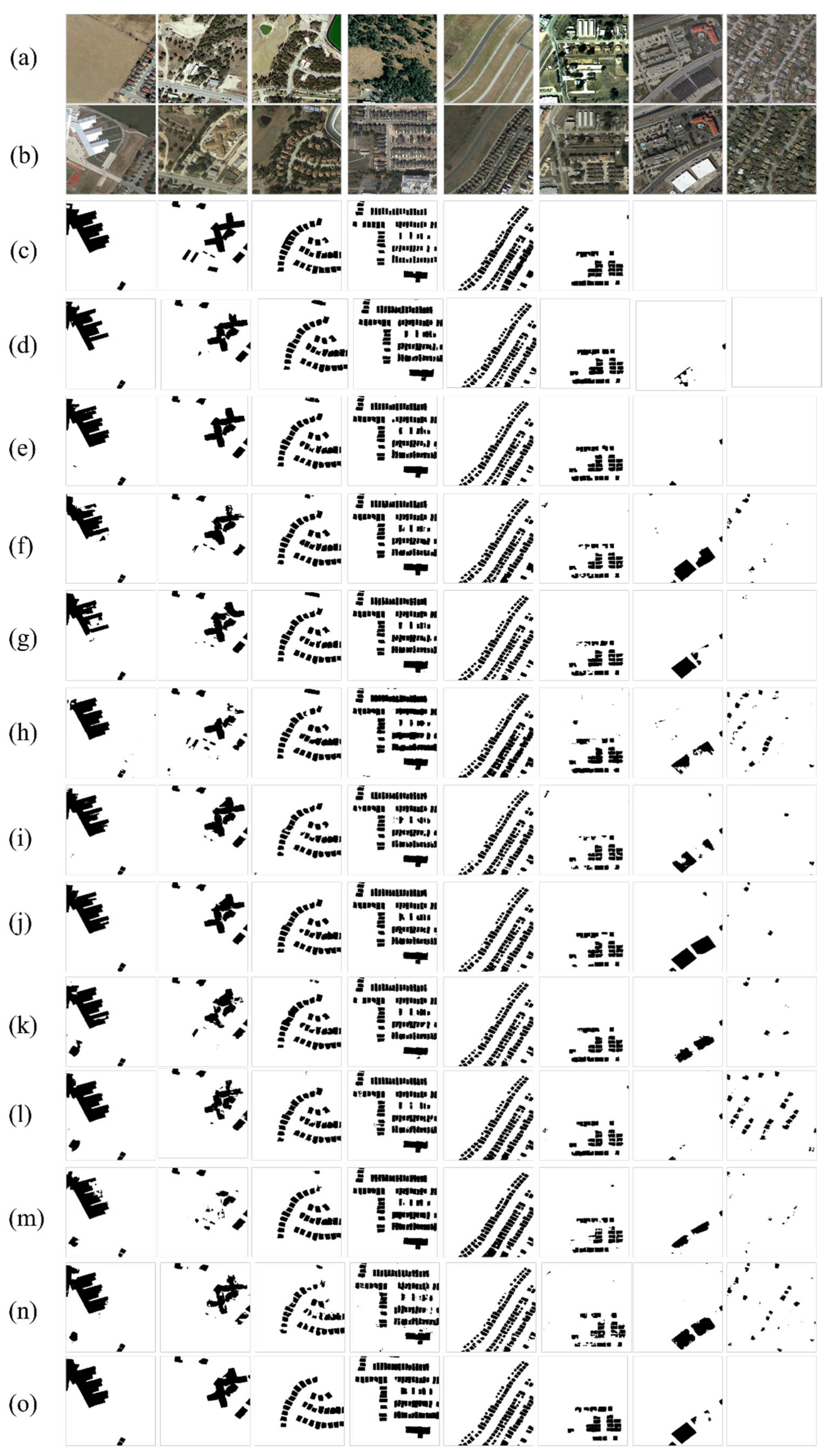
For intuitive comparisons, some change detection results are presented in Figure 4. For the LEVIR-CD dataset, the main change type lies in the building changes. Note that the black pixels indicate the changed buildings while the white pixels indicate the background regions. From the first two columns, we can observe that 1M-CDNet and 3M-CDNet generated more compact change masks. However, other approaches, such as DDCNN and the three U-shape-based variants, exhibit poor performance. Most of them generated change masks with holes and fragmentized boundaries. Specifically, as shown in the following columns, our 1M-CDNet and 3M-CDNet exhibit better performance on the detection of changed objects with small scales than other methods. 1M-CDNet and 3M-CDNet achieved higher recall than other methods, which is consistent with the quantitative analysis. 1M-CDNet and 3M-CDNet succeeded to discriminate the crowded building instances from each other. The main advantage owes to that we apply the DConv-based backbone network to extract high-resolution feature maps for change detection. From the last two columns, other approaches suffer from many false alarms of varying degrees due to the identical building roofs in bitemporal images exhibiting different colors. Instead, our 1M-CDNet and 3M-CDNet completely overcome the distractions and succeeds to identify the missed changed buildings in the reference maps as shown in the 7th column. We can conclude that 1M-CDNet and 3M-CDNet are more stable against pseudo-changes caused by spectral changes.

3.5.2. Comparisons on Season-Varying Dataset

(a) 
Quantitative evaluation
Table 6 presents the quantitative results on the Season-Varying dataset. Due to more challenges caused by season variations, FarSeg achieved third place and exhibited better performance than other FCN-based or attention-based approaches by modeling the foreground-correlated contexts. We can observe that our 1M-CDNet and 3M-CDNet consistently perform better than other benchmarks in terms of accuracy. For example, 1M-CDNet outperforms the lightweight CLNet with an increased IoU (0.56%) and F1 (0.30%), and that 3M-CDNet outperforms the lightweight CLNet with an increased IoU (1.87%) and F1 (0.99%). From Table 4, we can observe that 1M-CDNet only involves 1.26 M parameters, which are about 4% of FarSeg that requires 31.38 M. Nonetheless, 1M-CDNet achieved an improvement of IoU (+0.36%) and F1 (+0.20%) compared with FarSeg. Specifically, 1M-CDNet requires much fewer parameters than DDCNN and reduces the computational costs. Table 4 shows the number of parameters of DDCNN (60.21 M) is about 47 times that of 1M-CDNet, and DDCNN’s computational cost (214.16 GFLOPs) is about 46 times of 1M-CDNet. However, 1M-CDNet outperforms DDCNN with a significant margin of an increased F1 (+2.34%) and IoU (+4.28%). In addition, the models that require similar parameters to our 1M-CDNet exhibit poor performance on Season-Varying dataset, such as FC-Siam-Conc, FC-Siam-Diff, and FC-EF-Res. Their performance is limited to the insufficient model capacity.
(b) 
Qualitative evaluation
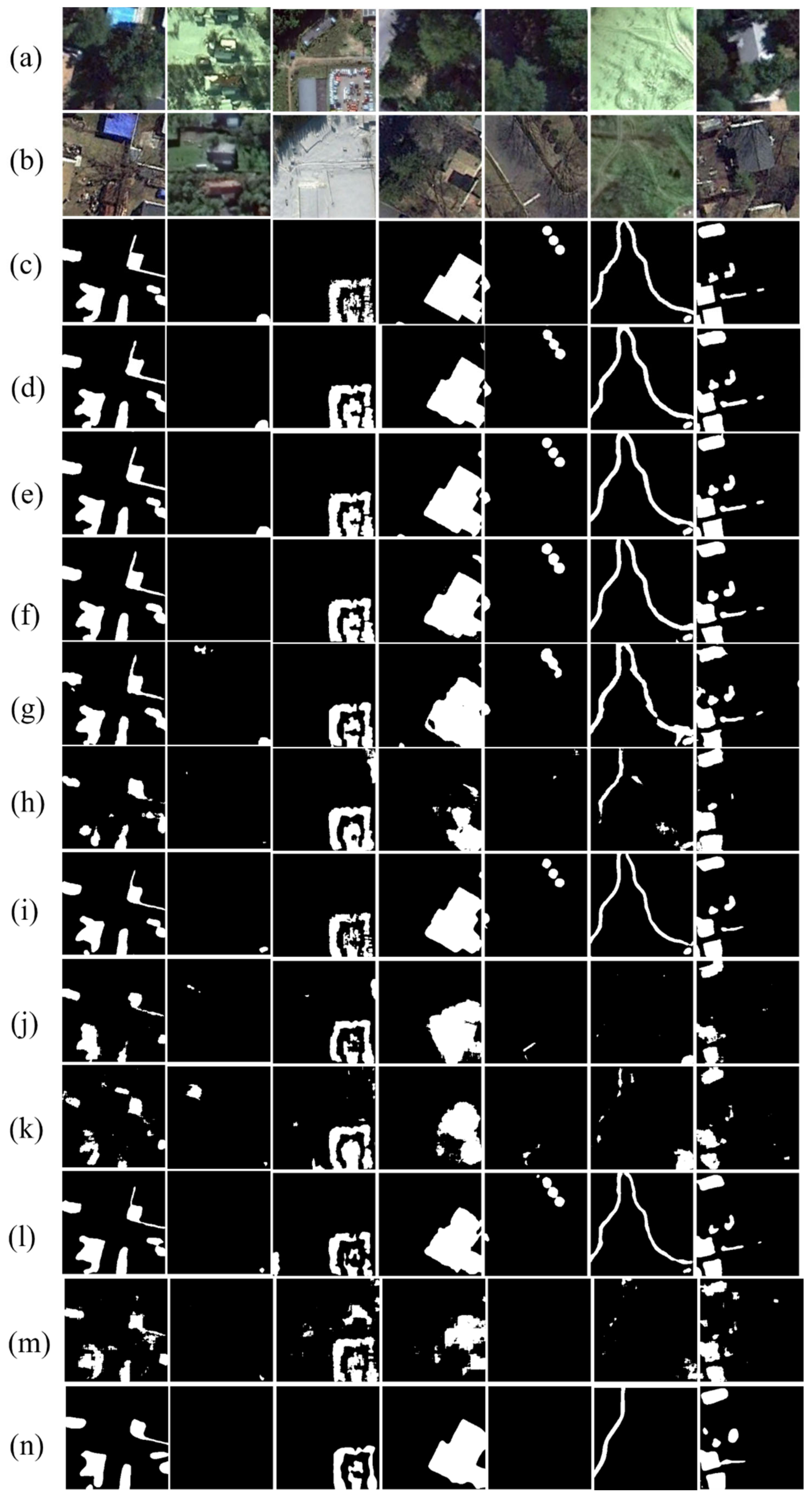
For the Season-Varying dataset, the change types are mainly related to land changes, building changes, road changes, and car changes. Some change results are shown in Figure 5. The black pixels indicate unchanged regions and the white pixels indicate the changed regions. Compared to other models, change masks generated by 1M-CDNet and 3M-CDNet preserve the actual shape of changed objects with more complete boundaries. However, change masks generated by other methods show fragmentized boundaries, such as FarSeg, STANet, CLNet, BIT-CD, and MSPP-Net, especially for large-scale geospatial objects with various shapes. Even worse, the other three U-shape-based variants exhibit a poor recall because they failed to detect the small changed objects in most cases. What is more, 1M-CDNet and 3M-CDNet generated promising change maps that are more robust to the spectral changes and vegetation growth caused by seasonal variations (e.g., from summer to winter/autumn).

4. Discussion

Ablation studies were conducted to verify each component’s contribution to 3M-CDNet. Table 7 and Table 8 present the quantitative results on two public datasets, where “w/o” and “w/” mean “without” and “with”, respectively.

4.1. Effectiveness of Different Multilevel Feature Fusion Strategies

Table 7 presents the effects of multilevel feature fusion strategies. Note that all these experiments were carried out by applying online data augmentation during training. Table 6 suggests that the two-level strategy always achieves the best performance in terms of F1 and IoU, i.e., LEVIR-CD (0.9161/0.8452) and Season-Varying (0.9749/0.9510). Compared with the one-level strategy that lacks low-level details, it increased IoU and F1 by about 2.09% and 1.24% on LEVIR-CD as well as 1.70% and 0.90% on Season-Varying, respectively. Unfortunately, the impact of the three-level strategy is negligible for model training. Compared with the one-level strategy, as shown on LEVIR-CD, the three-level strategy just help to achieve a little improvement of F1 (0.29%) and IoU (0.48%) as well as improvement of F1 (0.23%) and IoU (0.44%) on Season-Varying, respectively. We can conclude that the two-level strategy is enough for improvements in our case while introducing either insufficient or excessive features could bring about an unexpected degradation problem. Therefore, we employ the two-level strategy for feature fusion in the experiments.

4.2. Effects of Online DA, Dropout, and Dconv

Table 8 presents the effectiveness of core components of 3M-CDNet. In Table 8, the first row shows 3M-CDNet’s quantitative results on LEVIR-CD and Season-Varying datasets, where 3M-CDNet adopted all these components, i.e., online DA, dropout, and DConv.
Online DA was used to simulate scale variations, illumination variations, and pseudo-changes caused by season variations. Table 8 suggests that online DA makes impressive contributions on both datasets, e.g., 3M-CDNet vs. w/o DA. Compared with the situation “w/o DA”, applying DA achieves considerable improvements of F1 (1.43%) and IoU (2.40%) on LEVIR-CD, as well as F1 (0.78%) and IoU (1.47%) on Season-Varying. It demonstrates that the online DA strategy described in Section 3.3 (b) is an effective trick to achieve immediate gains through improving the diversity of samples, especially when lacking enough training samples, such as LEVIR-CD.
Meanwhile, dropout can be an effective complementary regularization with online DA for achieving a good generalization capacity. Compared with the results shown in “w/o DA/Dropout”, 3M-CDNet achieves improvements of F1 (2.05%) and IoU (3.43%) on LEVIR-CD, as well as F1 (0.95%) and IoU (1.69%) on Season-Varying. Dropout increased the F1 by 0.62% and IoU by 1.03% on LEVIR-CD, and as well as F1 (0.17%) and IoU (0.32%) on Season-Varying, even in the case of not using online DA (“w/o DA/Dropout” vs. “w/o DA”).
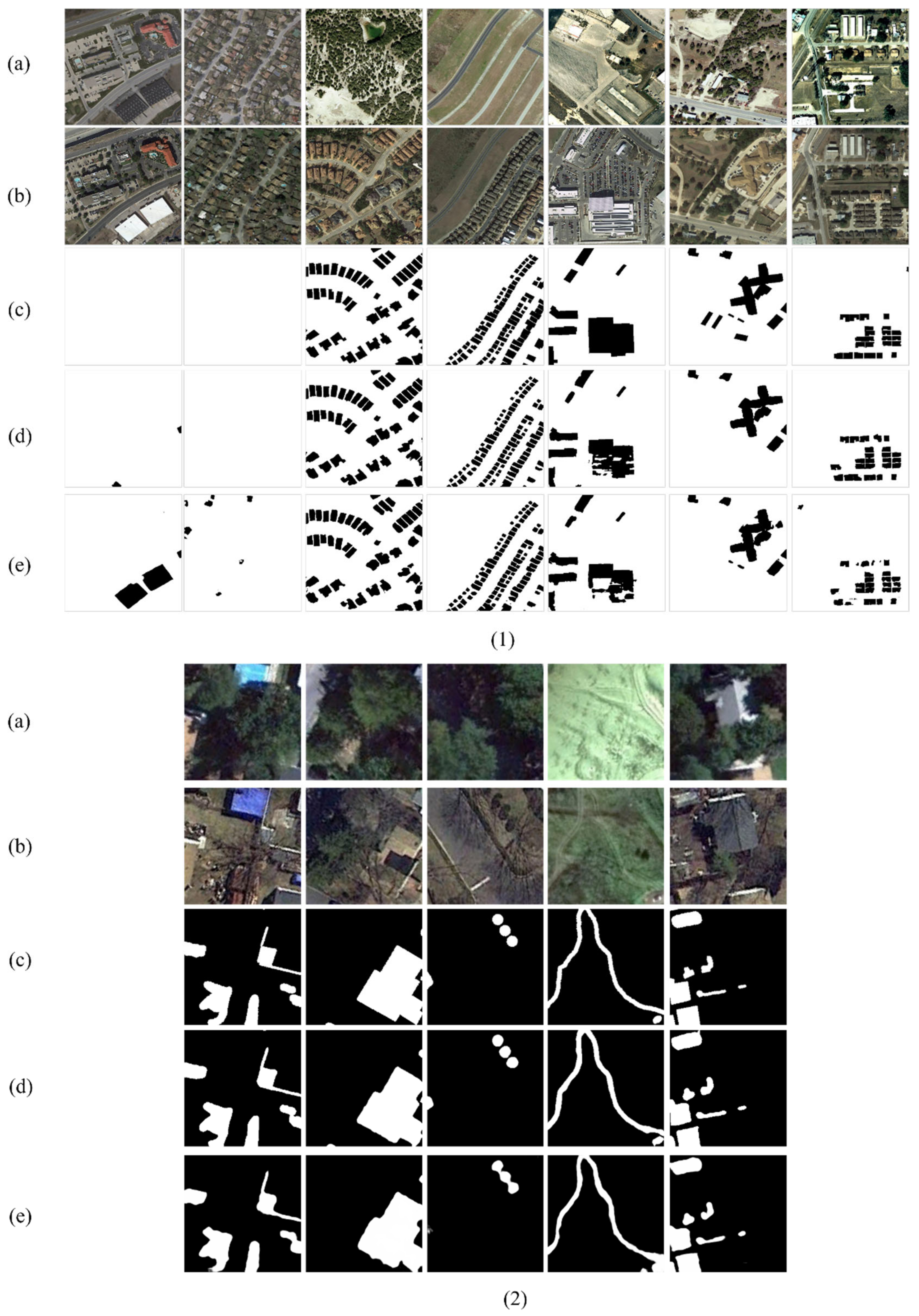
Last but not least, DConv was incorporated into the backbone network to enlarge the receptive field of deep features. Table 8 shows that DConv serves as an indispensable component for achieving high accuracy. For an instance, the last row shows that performance drops significantly without DConv (3M-CDNet vs. w/o DConv), where F1 decreased by about 1% and 1.38% on the two datasets, and IoU decreased by 1.69% and 2.59%, respectively. Moreover, DConv with online DA promoted the performance significantly and achieved improvements of F1 (+2.29%) and IoU (+3.83%) on LEVIR-CD (3M-CDNet vs. “w/o DA/DConv”). Since the Season-Varying dataset includes geospatial objects with various shapes and scales, 3M-CDNet achieved a significant margin compared with the situation “w/o DA/DConv”, i.e., F1 (+2.63%) and IoU (+4.89%) on Season-Varying. Thus, the DConv-based backbone promotes the geometric transformation modeling ability of our lightweight model. For intuitive comparisons, some detection results on both datasets were presented in Figure 6.
We can observe that change maps generated by 3M-CDNet are overall closer to the reference change map than that of “w/o DConv”. From the first two columns in Figure 6(1), 3M-CDNet presents a significant margin compared with the change maps of “w/o DConv”. The latter suffers from false alarms caused by the different colors of the identical building roofs. Meanwhile, 3M-CDNet achieved a higher detection rate on the objects with small scales, as shown in the last column of Figure 6(1). In addition, the changed building masks generated by 3M-CDNet have more complete smoother boundaries, as shown in Figure 6(1,2). Moreover, 3M-CDNet could identify building instances from the crowded buildings, as shown in the 3rd and 4th columns of Figure 6(1). What is more, the season changes between bi-temporal images significantly vary, such as season changes of natural objects (i.e., from wide forest areas to single trees). However, during the generation of reference maps, only the appearance and disappearance were considered as image changes while ignoring changes due to season differences, brightness, and other factors. 3M-CDNet generated promising change maps that show robustness to the spectral changes and vegetation growth caused by seasonal variations (e.g., from summer to winter/autumn), which is challenging for traditional methods.

5. Conclusions

In this paper, an effective network termed 3M-CDNet, and a lightweight variant termed 1M-CDNet, were proposed for urban change detection using bitemporal remote sensing images. The lightweight model was obtained by reducing the width and depth of the backbone network. We can conclude the proposed networks achieve performance improvements from the following perspectives. First, high-resolution feature maps extracted by the backbone network facilitate the detection of small changed objects with acceptable computational costs. Second, the backbone network was incorporated with deformable convolutions to promote the geometric transformation modeling ability of our lightweight model. In addition, the two-level feature fusion strategy was applied to improve the feature representation. Finally, dropout applied in the classifier and online data augmentation bring about immediate gains without extra cost. What is more, the proposed networks allow us to flexibly adjust the classifier to satisfy different trade-offs between accuracy and efficiency in practice.
Extensive experiments have verified the effectiveness of the 1M-CDNet and 3M-CDNet. Experiment results have shown that 1M-CDNet and 3M-CDNet exhibited better performance compared with the state-of-the-art approaches. For example, 1M-CDNet achieved the F1 (0.9118) and IoU (0.8379) on LEVIR-CD dataset, as well as the F1 (0.9680) and IoU (0.9379) on the Season-Varying dataset. Additionally, 3M-CDNet achieved the best F1 (0.9161) and IoU (0.8452) on the LEVIR-CD dataset, as well as the best F1 (0.9749) and IoU (0.9510) on the Season-Varying dataset. Specifically, 1M-CDNet makes a better trade-off between accuracy and inference speed compared with existing methods. Future works will focus on further improving detection accuracy and reducing the computational costs by incorporating some model compression techniques, such as knowledge distillation and channel pruning techniques.

Author Contributions

K.S. conceived the paper, designed and performed the experiments, and wrote the paper. F.C. performed some experiments. K.S. and F.C. completed the visualization. J.J. supervised the study and modified the paper. All authors have read and agreed to the published version of the manuscript.

Funding

This research was supported by the National Natural Science Foundation of China (No. 61725501).

Acknowledgments

This article is supported by the Key Laboratory of Precision Opto-mechatronics Technology, Ministry of Education, Beihang University, China.

Conflicts of Interest

The authors declare no conflict of interest.

References

  1. Long, Y.; Xia, G.S.; Li, S.; Yang, W.; Yang, M.Y.; Zhu, X.X.; Zhang, L.; Li, D. On Creating Benchmark Dataset for Aerial Image Interpretation: Reviews, Guidances, and Million-AID. Int. J. Remote Sens. 2021, 14, 4205–4230. [Google Scholar] [CrossRef]
  2. Singh, A. Review Article Digital change detection techniques using remotely-sensed data. Int. J. Remote Sens. 1989, 10, 989–1003. [Google Scholar] [CrossRef] [Green Version]
  3. Bouziani, M.; Goïta, K.; He, D.-C. Automatic change detection of buildings in urban environment from very high spatial resolution images using existing geodatabase and prior knowledge. ISPRS J. Photogramm. Remote Sens. 2010, 65, 143–153. [Google Scholar] [CrossRef]
  4. Deng, J.S.; Wang, K.; Deng, Y.H.; Qi, G.J. PCA-based land-use change detection and analysis using multitemporal and multisensor satellite data. Int. J. Remote Sens. 2008, 29, 4823–4838. [Google Scholar] [CrossRef]
  5. Gupta, R.; Hosfelt, R.; Sajeev, S.; Patel, N.; Goodman, B.; Doshi, J.; Heim, E.; Choset, H.; Gaston, M. xBD: A Dataset for Assessing Building Damage from Satellite Imagery. In Proceedings of the IEEE/CVF Conference on Computer Vision and Pattern Recognition (CVPR) Workshops, Long Beach, CA, USA, 16–20 June 2019; pp. 10–17. [Google Scholar]
  6. Shi, W.; Min, Z.; Zhang, R.; Chen, S.; Zhan, Z. Change Detection Based on Artificial Intelligence: State-of-the-Art and Challenges. Int. J. Remote Sens. 2020, 12, 1688. [Google Scholar] [CrossRef]
  7. Xiao, P.; Zhang, X.; Wang, D.; Yuan, M.; Feng, X.; Kelly, M. Change detection of built-up land: A framework of combining pixel-based detection and object-based recognition. ISPRS J. Photogramm. Remote Sens. 2016, 119, 402–414. [Google Scholar] [CrossRef]
  8. Hussain, M.; Chen, D.; Cheng, A.; Wei, H.; Stanley, D. Change detection from remotely sensed images: From pixel-based to object-based approaches. ISPRS J. Photogramm. Remote Sens. 2013, 80, 91–106. [Google Scholar] [CrossRef]
  9. Chen, J.; Gong, P.; He, C.; Pu, R.; Shi, P. Land-Use/Land-Cover Change Detection Using Improved Change-Vector Analysis. ISPRS J. Photogramm. Remote Sens. 2003, 69, 369–379. [Google Scholar] [CrossRef] [Green Version]
  10. Nielsen, A.A. The Regularized Iteratively Reweighted MAD Method for Change Detection in Multi- and Hyperspectral Data. IEEE Trans. Image Process. 2007, 16, 463–478. [Google Scholar] [CrossRef] [Green Version]
  11. Liu, Q.; Liu, L. Unsupervised Change Detection for Multispectral Remote Sensing Images Using Random Walks. Int. J. Remote Sens. 2017, 9, 438. [Google Scholar] [CrossRef] [Green Version]
  12. Ghosh, A.; Mishra, N.S.; Ghosh, S. Fuzzy clustering algorithms for unsupervised change detection in remote sensing images. Inf. Sci. 2011, 181, 699–715. [Google Scholar] [CrossRef]
  13. Celik, T. Unsupervised Change Detection in Satellite Images Using Principal Component Analysis and k-Means Clustering. IEEE Geosci. Remote Sens. Lett. 2009, 6, 772–776. [Google Scholar] [CrossRef]
  14. Lv, P.; Zhong, Y.; Zhao, J.; Zhang, L. Unsupervised Change Detection Based on Hybrid Conditional Random Field Model for High Spatial Resolution Remote Sensing Imagery. IEEE Trans. Geosci. Remote Sens. 2018, 56, 4002–4015. [Google Scholar] [CrossRef]
  15. Han, Y.; Javed, A.; Jung, S.; Liu, S. Object-Based Change Detection of Very High Resolution Images by Fusing Pixel-Based Change Detection Results Using Weighted Dempster–Shafer Theory. Int. J. Remote Sens. 2020, 12, 983. [Google Scholar] [CrossRef] [Green Version]
  16. Tan, K.; Zhang, Y.; Wang, X.; Chen, Y. Object-Based Change Detection Using Multiple Classifiers and Multi-Scale Uncertainty Analysis. Int. J. Remote Sens. 2019, 11, 359. [Google Scholar] [CrossRef] [Green Version]
  17. Wang, X.; Liu, S.; Du, P.; Liang, H.; Xia, J.; Li, Y. Object-Based Change Detection in Urban Areas from High Spatial Resolution Images Based on Multiple Features and Ensemble Learning. Int. J. Remote Sens. 2018, 10, 276. [Google Scholar] [CrossRef] [Green Version]
  18. Touazi, A.; Bouchaffra, D. A k-Nearest Neighbor approach to improve change detection from remote sensing: Application to optical aerial images. In Proceedings of the 2015 15th International Conference on Intelligent Systems Design and Applications (ISDA), Marrakech, Morocco, 14–16 December 2015; pp. 98–103. [Google Scholar]
  19. Feng, W.; Sui, H.; Tu, J.; Huang, W.; Sun, K. A novel change detection approach based on visual saliency and random forest from multi-temporal high-resolution remote-sensing images. Int. J. Remote Sens. 2018, 39, 7998–8021. [Google Scholar] [CrossRef]
  20. Bovolo, F.; Bruzzone, L.; Marconcini, M. A Novel Approach to Unsupervised Change Detection Based on a Semisupervised SVM and a Similarity Measure. IEEE Trans. Geosci. Remote Sens. 2008, 46, 2070–2082. [Google Scholar] [CrossRef] [Green Version]
  21. Benedek, C.; Szirányi, T. Change Detection in Optical Aerial Images by a Multilayer Conditional Mixed Markov Model. IEEE Trans. Geosci. Remote Sens. 2009, 47, 3416–3430. [Google Scholar] [CrossRef] [Green Version]
  22. Wu, C.; Du, B.; Cui, X.; Zhang, L. A post-classification change detection method based on iterative slow feature analysis and Bayesian soft fusion. Remote Sens. Environ. 2017, 199, 241–255. [Google Scholar] [CrossRef]
  23. Hou, B.; Wang, Y.; Liu, Q. Change Detection Based on Deep Features and Low Rank. IEEE Geosci. Remote Sens. Lett. 2017, 14, 2418–2422. [Google Scholar] [CrossRef]
  24. Ronneberger, O.; Fischer, P.; Brox, T. U-Net: Convolutional Networks for Biomedical Image Segmentation. In Proceedings of the International Conference on Medical Image Computing and Computer-Assisted Intervention, Munich, Germany, 5–9 October 2015; Springer: Berlin/Heidelberg, Germany, 2015; pp. 234–241. [Google Scholar]
  25. Zhou, Z.; Rahman Siddiquee, M.M.; Tajbakhsh, N.; Liang, J. UNet++: A Nested U-Net Architecture for Medical Image Segmentation. In Proceedings of the Deep Learning in Medical Image Analysis and Multimodal Learning for Clinical Decision Support, Granada, Spain, 20 September 2018; pp. 3–11. [Google Scholar]
  26. Daudt, R.C.; Saux, B.L.; Boulch, A. Fully Convolutional Siamese Networks for Change Detection. In Proceedings of the 2018 25th IEEE International Conference on Image Processing (ICIP), Athens, Greece, 7–10 October 2018; pp. 4063–4067. [Google Scholar]
  27. Peng, D.; Zhang, Y.; Wanbing, G. End-to-End Change Detection for High Resolution Satellite Images Using Improved UNet++. Int. J. Remote Sens. 2019, 11, 1382. [Google Scholar] [CrossRef] [Green Version]
  28. Wang, D.; Chen, X.; Jiang, M.; Du, S.; Xu, B.; Wang, J. ADS-Net:An Attention-Based deeply supervised network for remote sensing image change detection. Int. J. Appl. Earth Obs. Geoinf. 2021, 101, 102348. [Google Scholar] [CrossRef]
  29. Zheng, Z.; Wan, Y.; Zhang, Y.; Xiang, S.; Peng, D.; Zhang, B. CLNet: Cross-layer convolutional neural network for change detection in optical remote sensing imagery. ISPRS J. Photogramm. Remote Sens. 2021, 175, 247–267. [Google Scholar] [CrossRef]
  30. Zhang, C.; Yue, P.; Tapete, D.; Jiang, L.; Shangguan, B.; Huang, L.; Liu, G. A deeply supervised image fusion network for change detection in high resolution bi-temporal remote sensing images. ISPRS J. Photogramm. Remote Sens. 2020, 166, 183–200. [Google Scholar] [CrossRef]
  31. Hou, B.; Liu, Q.; Wang, H. From W-Net to CDGAN: Bitemporal Change Detection via Deep Learning Techniques. IEEE Trans. Geosci. Remote Sens. 2019, 58, 1790–1802. [Google Scholar] [CrossRef] [Green Version]
  32. Woo, S.; Park, J.; Lee, J.-Y.; Kweon, I.S. CBAM: Convolutional Block Attention Module. In Proceedings of the Computer Vision—ECCV 2018, Munich, Germany, 8–14 September 2018; pp. 3–19. [Google Scholar]
  33. Fang, S.; Li, K.; Shao, J.; Li, Z. SNUNet-CD: A Densely Connected Siamese Network for Change Detection of VHR Images. IEEE Geosci. Remote Sens. Lett. 2021, 1–5. [Google Scholar] [CrossRef]
  34. Zhang, Y.; Fu, L.; Li, Y.; Zhang, Y. HDFNet: Hierarchical Dynamic Fusion Network for Change Detection in Optical Aerial Images. Int. J. Remote Sens. 2021, 13, 1440. [Google Scholar] [CrossRef]
  35. Caye Daudt, R.; Le Saux, B.; Boulch, A.; Gousseau, Y. Multitask learning for large-scale semantic change detection. Comput. Vis. Image. Underst. 2019, 187, 102783. [Google Scholar] [CrossRef] [Green Version]
  36. He, K.; Zhang, X.; Ren, S.; Sun, J. Deep Residual Learning for Image Recognition. In Proceedings of the 2016 IEEE Conference on Computer Vision and Pattern Recognition (CVPR), Las Vegas, NV, USA, 27–30 June 2016; pp. 770–778. [Google Scholar]
  37. Peng, X.; Zhong, R.; Li, Z.; Li, Q. Optical Remote Sensing Image Change Detection Based on Attention Mechanism and Image Difference. IEEE Trans. Geosci. Remote Sens. 2020, 59, 7296–7307. [Google Scholar] [CrossRef]
  38. Zhang, X.; Yue, Y.; Gao, W.; Yun, S.; Su, Q.; Yin, H.; Zhang, Y. DifUnet++: A Satellite Images Change Detection Network Based on Unet++ and Differential Pyramid. IEEE Geosci. Remote Sens. Lett. 2021, 1–5. [Google Scholar] [CrossRef]
  39. Yu, X.; Fan, J.; Chen, J.; Zhang, P.; Zhou, Y.; Han, L. NestNet: A multiscale convolutional neural network for remote sensing image change detection. Int. J. Remote Sens. 2021, 42, 4902–4925. [Google Scholar] [CrossRef]
  40. Vaswani, A.; Shazeer, N.; Parmar, N.; Uszkoreit, J.; Jones, L.; Gomez, A.; Kaiser, L.; Polosukhin, I. Attention Is All You Need. In Proceedings of the Advances in Neural Information Processing Systems, Long Beach, CA, USA, 4–9 December 2017; pp. 5998–6008. [Google Scholar]
  41. Wang, X.; Girshick, R.B.; Gupta, A.; He, K. Non-Local Neural Networks. In Proceedings of the IEEE Conference on Computer Vision and Pattern Recognition, Salt Lake City, UT, USA, 18–22 June 2018; pp. 7794–7803. [Google Scholar]
  42. Hu, J.; Shen, L.; Albanie, S.; Sun, G.; Wu, E. Squeeze-and-Excitation Networks. IEEE Trans. Pattern. Anal. Mach. Intell. 2020, 42, 2011–2023. [Google Scholar] [CrossRef] [PubMed] [Green Version]
  43. Fu, J.; Liu, J.; Tian, H.; Li, Y.; Bao, Y.; Fang, Z.; Lu, H. Dual Attention Network for Scene Segmentation. In Proceedings of the 2019 IEEE/CVF Conference on Computer Vision and Pattern Recognition (CVPR), Long Beach, CA, USA, 15–20 June 2019; pp. 3141–3149. [Google Scholar]
  44. Chen, H.; Shi, Z. A Spatial-Temporal Attention-Based Method and a New Dataset for Remote Sensing Image Change Detection. Int. J. Remote Sens. 2020, 12, 1662. [Google Scholar] [CrossRef]
  45. Dosovitskiy, A.; Beyer, L.; Kolesnikov, A.; Weissenborn, D.; Zhai, X.; Unterthiner, T.; Dehghani, M.; Minderer, M.; Heigold, G.; Gelly, S.; et al. An Image is Worth 16 × 16 Words: Transformers for Image Recognition at Scale. arXiv 2020, arXiv:2010.11929. [Google Scholar]
  46. Zhu, X.; Su, W.; Lu, L.; Li, B.; Wang, X.; Dai, J. Deformable DETR: Deformable Transformers for End-to-End Object Detection. In Proceedings of the International Conference on Learning Representations, Vienna, Austria, 4 May 2021. [Google Scholar]
  47. Zheng, S.; Lu, J.; Zhao, H.; Zhu, X.; Luo, Z.; Wang, Y.; Fu, Y.; Feng, J.; Xiang, T.; Torr, P.; et al. Rethinking Semantic Segmentation from a Sequence-to-Sequence Perspective with Transformers. In Proceedings of the IEEE/CVF Conference on Computer Vision and Pattern Recognition (CVPR), Nashville, TN, USA, 20–25 June 2021; pp. 6881–6890. [Google Scholar]
  48. Chen, H.; Qi, Z.; Shi, Z. Remote Sensing Image Change Detection With Transformers. IEEE Trans. Geosci. Remote Sens. 2021, 10, 1–14. [Google Scholar] [CrossRef]
  49. Chen, J.-W.; Wang, R.; Ding, F.; Liu, B.; Jiao, L.; Zhang, J. A Convolutional Neural Network with Parallel Multi-Scale Spatial Pooling to Detect Temporal Changes in SAR Images. Remote Sens. 2020, 12, 1619. [Google Scholar] [CrossRef]
  50. Wang, R.; Ding, F.; Chen, J.W.; Jiao, L.; Wang, L. A Lightweight Convolutional Neural Network for Bitemporal Image Change Detection. In Proceedings of the IGARSS 2020—2020 IEEE International Geoscience and Remote Sensing Symposium, Waikoloa, HI, USA, 26 September–2 October 2020; pp. 2551–2554. [Google Scholar]
  51. Dai, J.; Qi, H.; Xiong, Y.; Li, Y.; Zhang, G.; Hu, H.; Wei, Y. Deformable Convolutional Networks. In Proceedings of the 2017 IEEE International Conference on Computer Vision (ICCV), Venice, Italy, 22–29 October 2017; pp. 764–773. [Google Scholar]
  52. Zhu, X.; Hu, H.; Lin, S.; Dai, J. Deformable ConvNets V2: More Deformable, Better Results. In Proceedings of the 2019 IEEE/CVF Conference on Computer Vision and Pattern Recognition (CVPR), Long Beach, CA, 15–20 June 2019; pp. 9300–9308. [Google Scholar]
  53. Srivastava, N.; Hinton, G.; Krizhevsky, A.; Sutskever, I.; Salakhutdinov, R. Dropout: A Simple Way to Prevent Neural Networks from Overfitting. J. Mach. Learn. Res. 2014, 15, 1929–1958. [Google Scholar]
  54. Bolya, D.; Zhou, C.; Xiao, F.; Lee, Y. YOLACT++: Better Real-time Instance Segmentation. IEEE Trans. Pattern. Anal. Mach. Intell. 2020. [Google Scholar] [CrossRef]
  55. Lebedev, M.; Vizilter, Y.; Vygolov, O.; Knyaz, V.; Rubis, A. Change Detection in Remote Sensing Images Using Conditional Advertisal Networks. Int. Arch. Photogramm. Remote Sens. 2018, 42, 565–571. [Google Scholar] [CrossRef] [Green Version]
  56. Paszke, A.; Gross, S.; Massa, F.; Lerer, A.; Bradbury, J.; Chanan, G.; Killeen, T.; Lin, Z.; Gimelshein, N.; Antiga, L.; et al. PyTorch: An Imperative Style, High-Performance Deep Learning Library. In Proceedings of the NeurlPS, Vancouver, BC, Canada, 8–11 December 2019. [Google Scholar]
  57. Loshchilov, I.; Hutter, F. Decoupled Weight Decay Regularization. In Proceedings of the ICLR, New Orleans, LA, USA, 6–9 May 2019. [Google Scholar]
  58. Zheng, Z.; Zhong, Y.; Wang, J.; Ma, A. Foreground-Aware Relation Network for Geospatial Object Segmentation in High Spatial Resolution Remote Sensing Imagery. In Proceedings of the 2020 IEEE/CVF Conference on Computer Vision and Pattern Recognition (CVPR), Seattle, WA, USA, 13–19 June 2020; pp. 4095–4104. [Google Scholar]
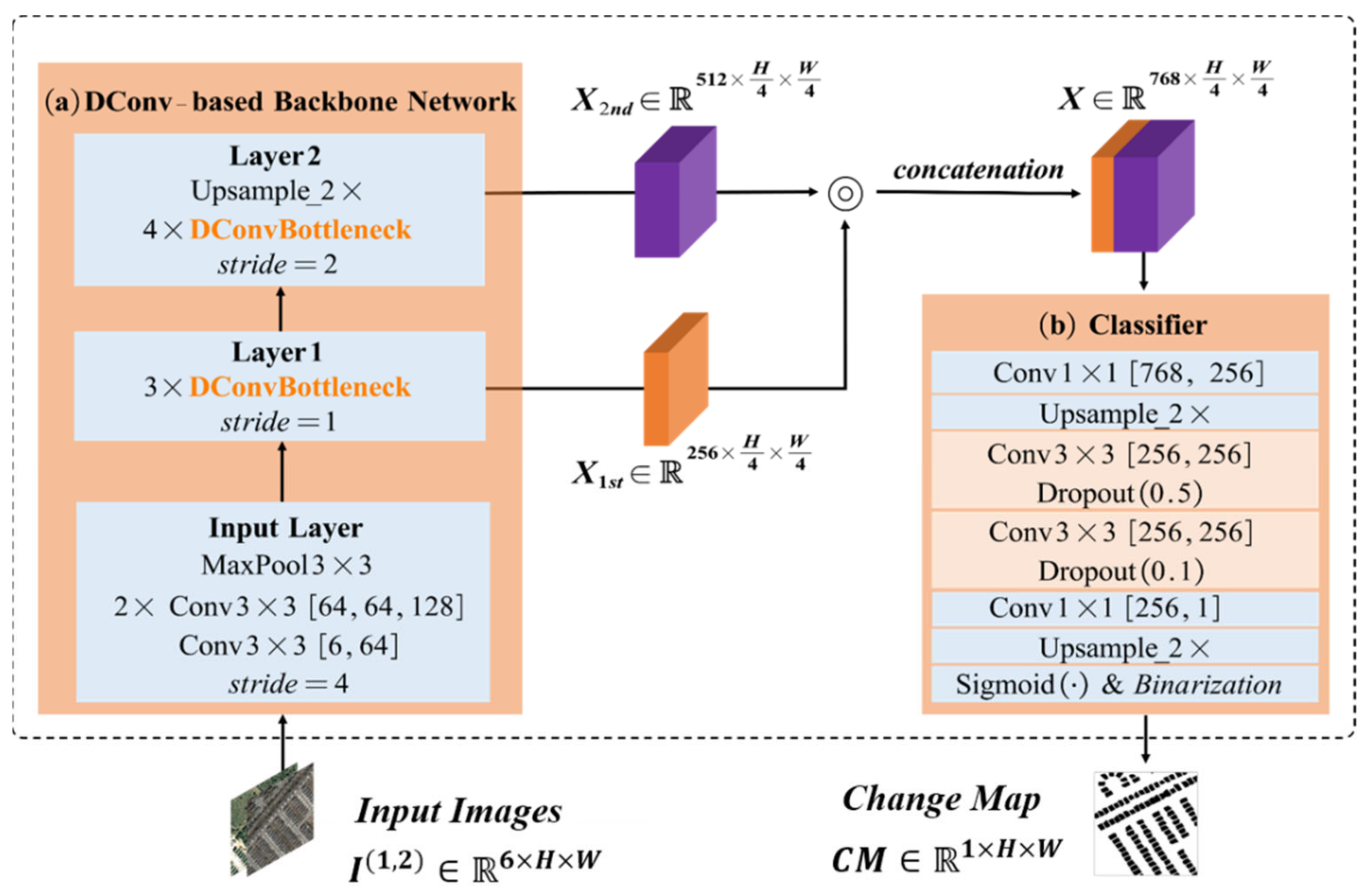
Figure 1. Workflow of the proposed change detection network.
Remotesensing 13 05152 g001
Figure 2. Architecture of the bottleneck residual blocks. Convolution layers are denoted by “number of kernels of each filter, kernel size, number of filters”, e.g., “128, Conv1 × 1, 64”. Conv and DConv indicate the 2-D convolution layer and deformable convolution layer, respectively. (a) Structure of Layer1_1. (b) Structure of Layer1_2 and Layer1_3. (c) Structure of Layer2_1. (d) Structure of Layer2_2, Layer2_3, and Layer2_4.
Remotesensing 13 05152 g002
Figure 3. Implementation of deformable convolutions.
Remotesensing 13 05152 g003
Figure 4. CD results of 3M-CDNet and other benchmarks on the LEVIR-CD dataset. Zoom in for an improved view. (a) Image T1. (b) Image T2. (c) Reference change map. (d) 1M-CDNet. (e) 3M-CDNet. (f) DDCNN. (g) FarSeg. (h) STANet. (i) FC-EF-Res. (j) CLNet. (k) FC-Siam-diff. (l) FC-Siam-conc. (m) BIT-CD. (n) MSPP-Net. (o) Lite-CNN.
Remotesensing 13 05152 g004
Figure 5. CD results of 3M-CDNet and other benchmarks on the Season-Varying dataset. Zoom in for an improved view. (a) Image T1. (b) Image T2. (c) Reference change map. (d) 1M-CDNet. (e) 3M-CDNet. (f) FarSeg. (g) STANet. (h) FC-EF-Res. (i) CLNet. (j) FC-Siam-diff. (k) FC-Siam-conc. (l) BIT-CD. (m) MSPP-Net. (n) Lite-CNN.
Remotesensing 13 05152 g005
Figure 6. CD results of 3M-CDNet and that of w/o DConv on the LEVIR-CD dataset (1) and the Season-Varying dataset (2). Zoom in for an improved view. (a) Image T1. (b) Image T2. (c) Reference change map. (d) 3M-CDNet. (e) w/o Dconv.
Remotesensing 13 05152 g006
Table 1. The detailed architecture of the backbone network.
Layer NameComponents, Kernel Size, FiltersStride Output   C × H × W
Input Layer C o n v 1 ,   3 × 3 ,   64 2 64 × 256 × 256
C o n v 2 _ 1 ,   3 × 3 ,   64 1 64 × 256 × 256
C o n v 2 _ 2 ,   3 × 3 ,   128 1 128 × 256 × 256
MaxPool ,   3 × 3 ,   128 2 128 × 128 × 128
Layer1 Layer 1 _ x   C o n v ,   1 × 1 ,   64   D C o n v ,   3 × 3 ,   64 C o n v ,   1 × 1 ,   256 × 3 1 256 × 128 × 128
Layer2 Layer 2 _ x   C o n v ,   1 × 1 ,   128   D C o n v ,   3 × 3 ,   128 C o n v ,   1 × 1 ,   512 × 4 2 512 × 64 × 64
Layer2_Upsample_2×, —, — 512 × 128 × 128
Table 2. The detailed architecture of the 3M-CDNet classifier.
Layer NameComponents, Kernel Size, FiltersStride Output   C × H × W
Classifier C o n v 3 _ 1 ,   1 × 1 ,   256 1 256 × 128 × 128
Upsample_2× 256 × 256 × 256
C o n v 3 _ 2 ,   3 × 3 ,   256 1 256 × 256 × 256
Dropout_0.5 256 × 256 × 256
C o n v 3 _ 3 ,   3 × 3 ,   256 1 256 × 256 × 256
Dropout_0.1 256 × 256 × 256
C o n v 3 _ 4 ,   1 × 1 ,   1 1 1 × 256 × 256
Upsample_2× 1 × 512 × 512
Sigmoid 1 × 512 × 512
Table 3. The detailed architecture of the 1M-CDNet classifier.
Layer NameComponents, Kernel Size, FiltersStride Output   C × H × W
Classifier C o n v 3 _ 1 ,   1 × 1 ,   256 1 256 × 128 × 128
Upsample_2× 256 × 256 × 256
Dropout_0.5256 × 256 × 256
C o n v 3 _ 2 ,   1 × 1 , 64 164 × 256 × 256
Dropout_0.164 × 256 × 256
C o n v 3 _ 3 ,   1 × 1 , 1 1 1 × 256 × 256
Upsample_2× 1 × 512 × 512
Sigmoid 1 × 512 × 512
Table 4. Comparison of network parameters, computational costs, and runtime.
MethodNumber of Parameters (M)Computational Costs (GFLOPs) w/bs = 1Runtime (ms)
w/bs = 1
Runtime (ms)
w/bs = 16
512 × 512256 × 256512 × 512256 × 256512 × 512256 × 256
DDCNN [37]60.21856.63214.16151.0744.67-477.73
STANet [44]16.93206.6832.4212.0711.49--
FarSeg [56]31.3847.4511.8613.718.79168.5544.68
CLNet [29]8.5335.658.9111.124.92128.4633.22
BIT-CD [48]3.0562.6815.6716.2212.89259.1565.24
FC-Siam-Diff [26]1.3520.745.188.724.05128.4632.30
FC-Siam-Conc [26]1.5520.755.198.733.77130.1932.32
FC-EF-Res [35]1.106.941.737.734.8590.9823.78
MSPP-Net [49]6.24566.1616.5413.386.42186.6647.58
Lite-CNN [50]3.87619.174.7910.159.76116.7829.49
1M-CDNet1.2618.434.618.024.07126.7933.58
3M-CDNet3.1294.8323.7116.627.28327.6055.65
Table 5. Comparison of results on the LEVIR-CD dataset.
MethodPr (%)Re (%)OA (%)IoUF1
STANet [44]85.0191.3898.740.78690.8808
FC-EF-Res [35]91.4888.0498.970.81370.8973
FC-Siam-Conc [26]89.4989.1898.920.80720.8933
FC-Siam-Diff [26]91.2588.1898.970.81300.8969
BIT-CD [48]90.3889.6998.990.81870.9003
DDCNN [37]92.1589.0799.060.82790.9059
FarSeg [56]91.0490.2299.050.82860.9063
CLNet [29]90.8590.5399.050.82970.9069
MSPP-Net [48]89.6586.7398.810.78830.8816
Lite-CNN [49]90.7789.9699.020.82420.9036
1M-CDNet92.3290.0699.110.83790.9118
3M-CDNet91.9991.2499.150.84520.9161
Table 6. Comparison of results on the Season-Varying dataset.
MethodPr (%)Re (%)OA(%)IoUF1
FC-Siam-Conc [26]91.9482.0696.900.76560.8672
FC-Siam-Diff [26]93.9881.0597.020.77050.8704
FC-EF-Res [35]89.9187.3797.250.79560.8862
BIT-CD [48]98.4992.3498.880.91050.9531
STANet [44]93.1393.5998.360.87550.9336
DDCNN [37]96.7192.3298.640.89510.9446
CLNet [29]98.6294.4699.150.93230.9650
FarSeg [56]95.1298.1399.150.93430.9660
MSPP-Net [49]92.9585.9397.460.80670.8930
Lite-CNN [50]96.5889.7698.340.87000.9305
1M-CDNet95.0598.6199.190.93790.9680
3M-CDNet95.8899.1699.370.95100.9749
Table 7. Comparisons of the effects of multilevel feature fusion strategies.
MethodLEVIR-CDSeason-Varying
OA (%)IoUF1OA (%)IoUF1
w/two-level99.150.84520.916199.370.95100.9749
w/one-level99.030.82430.903799.140.93400.9659
w/three-level99.050.82910.906699.200.93840.9682
Table 8. The contribution of DA, Dropout, and DConv on the performance.
MethodLEVIR-CDSeason-Varying
OA (%)IoUF1OA (%)IoUF1
3M-CDNet99.150.84520.916199.370.95100.9749
w/o DA99.010.82120.901899.180.93630.9671
w/o DA/Dropout98.950.81090.895699.130.93310.9654
w/o DA/DConv98.920.80690.893298.730.90210.9486
w/o DConv99.040.82830.906199.020.92510.9611
Publisher’s Note: MDPI stays neutral with regard to jurisdictional claims in published maps and institutional affiliations.