Article

Analysis on Land-Use Change and Its Driving Mechanism in Xilingol, China, during 2000–2020 Using the Google Earth Engine

1
State Key Laboratory of Resources and Environmental Information System, Institute of Geographic Sciences and Natural Resources Research, Chinese Academy of Sciences, Beijing 100101, China
2
College of Natural Resources and Environment, Northwest A&F University, Yangling 712100, China
3
College of Resources and Environment, University of Chinese Academy of Sciences, Beijing 100049, China
4
Institute of Desertification Studies, Chinese Academy of Forestry, Beijing 100091, China
*
Author to whom correspondence should be addressed.
Remote Sens. 2021, 13(24), 5134; https://doi.org/10.3390/rs13245134
Submission received: 17 November 2021 / Revised: 10 December 2021 / Accepted: 14 December 2021 / Published: 17 December 2021

Abstract

:
Large-scale, long time-series, and high-precision land-use mapping is the basis for assessing the evolution and sustainability of ecosystems in Xilingol, the Inner Mongolia Autonomous Region, China. Based on Google Earth Engine (GEE) and Landsat satellite remote-sensing images, the random forest (RF) classification algorithm was applied to create a yearly land-use/land-cover change (LULC) dataset in Xilingol during the past 20 years (2000–2020) and to examine the spatiotemporal characteristics, dynamic changes, and driving mechanisms of LULC using principal component analysis and multiple linear stepwise regression methods. The main findings are summarized as follows. (1) The RF classification algorithm supported by the GEE platform enables fast and accurate acquisition of the LULC dataset, and the overall accuracy is 0.88 ± 0.01. (2) The ecological condition across Xilingol has improved significantly in the last 20 years (2000–2020), and the area of vegetation (grassland and woodland) has increased. Specifically, the area of high-coverage grass and woodland increases (+13.26%, +1.19%), while the area of water and moderate- and low-coverage grass decreases (−15.96%, −7.23%, and −3.27%). Cropland increases first and then decreases (−34.85%) and is mainly distributed in the southeast. The area of deserted land decreases in the south and increases in the center and north, but the total area still decreases (−13.74%). The built-up land expands rapidly (+108.45%). (3) In addition, our results suggest that regional socioeconomic development factors are the primary causes of changes in built-up land, and climate-related factors are the primary causes of water changes, but the correlations between other land-use types and relevant factors are not significant (cropland and grassland). We conclude that the GEE+RF method is capable of automated, long time-series, and high-accuracy land-use mapping, and further changes in climatic, environmental, and socioeconomic development factors, i.e., climate warming and rotational grazing, might have significant implications on regional land surface morphology and landscape dynamics.

1. Introduction

Land-use/land-cover change (LULC) plays a key role in the study of global climate change, food security, ecological restoration, and governance and has received widespread attention from governments and scientists around the world [1,2,3]. LULC is a direct consequence of human and nature interactions [4] and is influenced by multiple behavioral and structural factors, i.e., demand, technical capacity, social relationships, and natural environment [5]. On the one hand, the physical environment (topography, landscape, temperature, precipitation, etc.) is the underlying element that determines the spatial distribution patterns of LULC and significantly influences changes in surface patterns and landscape dynamics at long time scales [6,7]. On the other hand, various human-imposed land-development activities, such as agricultural exploitation and urbanization, not only change the regional land-use structure and landscape ecological patterns at the local scale but also accelerate global warming through increased greenhouse gas emissions [8,9,10]. In addition, large land-use changes often significantly affect ecosystem service supply, such as soil carbon pool change, soil fertility decline, water supply capacity decline, forest disaster risk increase, and biodiversity loss, leading to greater vulnerability to ecosystem services [11,12,13]. In urban areas, land-use change also severely affects the quality of urban human settlements, such as the formation of the urban heat island effect and urban waterlogging disasters [14].
At global or regional scales, the occurrence of disturbance events associated with land-use change generally alters the spectral properties of the land surface radically, making it easier to identify in Landsat imagery [15]. To perform high-precision remote-sensing monitoring of large-scale LULC over a long period and identify spatial patterns and dynamic changes, it is necessary to continuously improve land-use classification and mapping methods [16,17]. Satellite remote-sensing image classification and mapping methods can be generally classified into supervised classification, unsupervised classification, image segmentation, and deep learning. The dominant supervised classification algorithms include maximum likelihood (MLC), categorical regression decision tree (CART), random forest (RF), artificial neural network (ANN), and support vector machine (SVM) methods [18,19]. Among them, the RF method was proposed by Breiman in 2001 and has been widely used in ecosystem and land-use classification [20,21,22]. Akar et al. compared the classification results obtained by different algorithms based on the RF, SVM, and MLC using IKONOS and QuickBird images with different spatial resolutions and scene features. The results showed that for IKONOS images in the urban areas, the RF algorithm presented a classification accuracy 10% higher than SVM and 14% higher than SVM; for QuickBird images in the rural areas, the RF algorithm also showed the highest classification accuracy [23]. In the past, RF-based image classification studies were limited by computing power and storage space, which commonly only allowed the input of limited wavelength bands from multispectral images and rarely applied the full wavelength band from multispectral and hyperspectral satellite images. In addition, relatively few studies have introduced spatial auxiliary elements such as the NDVI (Normalized Difference Vegetation Index), NDWI (Normalized Difference Water Index), Digital Elevation Model (DEM), and Nighttime Light Index, which strongly reflect the spatiotemporal dynamics of the geographic environment and human activity elements. Therefore, the strengths of RF methods in processing multi-dimensional feature data have not been fully exploited. The emergence and development of satellite remote-sensing cloud storage and cloud computing platforms represented by the Google Earth Data Engine (GEE: Google Earth Engine) not only makes it possible to integrate multi-source and multi-scale global remote-sensing images but also allows for full-band and high-intensity image calculation [24]. Therefore, with the support of the GEE platform, the exploitation of the potential of classical algorithms such as MLC, ANN, RF, and SVM and the development of new deep-neural-network-based machine learning algorithms have become an important theme in the study field of LULC mapping at large scales [25,26,27].
Supported by continuous spatiotemporal datasets, the analysis of spatiotemporal patterns of LULC and the identification of driving mechanisms of environmental and anthropogenic activity factors gradually became the important prerequisites for sustainable development assessment, ecological restoration, and governance. Zewdie and Csaplovics analyzed the LULC in the semi-arid region of Ethiopia using Landsat MSS and Landsat TM data from 1970 to 2010 with SVM supervised classification algorithm and used socio-ecological survey to explore the driving forces, showing that agricultural land expansion, migration, and excessive deforestation were the most significant factors contributing to the loss of vegetation [28]. Hu et al. used the remote-sensing inversion products, including NPP and NDVI, to analyze the desertification sensitivity and long-term trends in Kazakhstan during 2000–2015 by a linear regression method; the results showed that the desertification process in the region was mainly driven by a warm–dry climate trend, and high-intensity pastoral development was another important factor contributing to desertification [29]. Liu et al. explored the spatial pattern of LULC in China during the early 21st century and its relationship with socioeconomic development factors, based on a 1 km dataset of LULC in China for every five years from 1995 to 2010. They found the implementation of regional development strategies such as “Western Development” and “Revitalization of Northeast China” were the main driving factors of LULC during that period [30]. The above studies provide fundamental spatial datasets for assessing regional sustainable development and propose specific policy rationales for protecting ecosystem services and reducing extreme environmental hazards in the context of global climate change. Most of these studies used the empirical qualitative analysis or correlation-based statistical modeling to analyze driving mechanisms. These approaches are difficult to isolate the real, direct drivers from complex systems and have the problem of simplifying causation to correlations.
Xilingol is located in the southeastern part of the Inner Mongolia Plateau, the transition zone from the arid region of northwest China to the humid region of the east. In the second half of the 20th century, due to climate change and intensifying grazing and reclamation activities, the ecosystem of this region experienced serious degradation, highlighted by the degradation of grassland and sand, and intensified wind and sand activities, which further affected the capital Beijing and the entire North China region. In response, the Chinese Government has strengthened the protection and governance of the ecosystem in this region since 2000; deployed the “Beijing–Tianjin Sandstorm Source Control” Project; and implemented a series of initiatives, including the conversion of cropland to grassland, reforestation, rotation grazing, and grass–livestock balance [31,32]. Various scholars have studied the pattern of LULC and the driving mechanisms in the region. Batunacun et al. studied the spatiotemporal patterns of land-use in Xilingol from 1975 to 2015 based on Landsat MSS/TM/ETM+/OLI data by visual interpretation of computer aided satellite images; they found that the region was dominated by grassland degradation from 1975 to 2000, while grassland recovery was obvious from 2000 to 2015 [32]. Based on 1995 and 2000 LULC datasets, Xu et al. used typical correspondence analysis to examine the relationship between climate, topography, human activity factors and LULC in Xilingol, showing that the total annual rainfall, distance to the nearest settlement, and LULC are strongly correlated [33]. Zhao et al. applied MOD09A1 remote-sensing images from 2000 to 2013 to investigate the relationship between grassland changes and meteorological conditions and human activities in Xilingol; they found that the correlation between grassland and precipitation was significant [34]. These studies analyzed regional LULC and ecosystem characteristics parameters (e.g., NDVI, NPP, etc.) in different time-series, and applied empirically statistical modeling approaches to discuss the driving mechanisms. However, there are some limitations: (1) the lack of high-precision, automated, spatiotemporal continuous LULC datasets makes it difficult to meet the practical needs in terms of the current status of the study results; (2) comparative studies based on time transects, rather than trend analysis based on time-series, can cause serious cognitive bias due to the contingency and randomness of selection; (3) trend analyses based on indirect indicators such as NDVI cannot reflect significant changes in all land-use types; (4) in the traditional LULC driver mechanism analysis, researchers typically include all potential elements in a particular model (e.g., statistical correlation model) at once, and then identify the key factors and their impact on LULC. The above technical route might lead to problems of autocorrelation between factors and unreasonable exclusion of direct drivers.
In response to the above issues, our study aims to implement a long time-series, high-accuracy land-use mapping of Xilingol by using Landsat remote-sensing image data since 2000 with a random forest classification algorithm and then investigate the relationship between LULC and climate and regional socioeconomic development factors of Xilingol by using principal component analysis and multiple linear stepwise regression methods. The specific objectives of this research are:
  • To explore whether the GEE+RF method is capable of automated, long time-series, and high-accuracy land-use mapping;
  • To examine the spatial pattern and characteristics of LULC over the study period;
  • To investigate the relationship between LULC and explanatory variables, including climate factors and regional socioeconomic development factors in Xilingol.

2. Materials and Methods
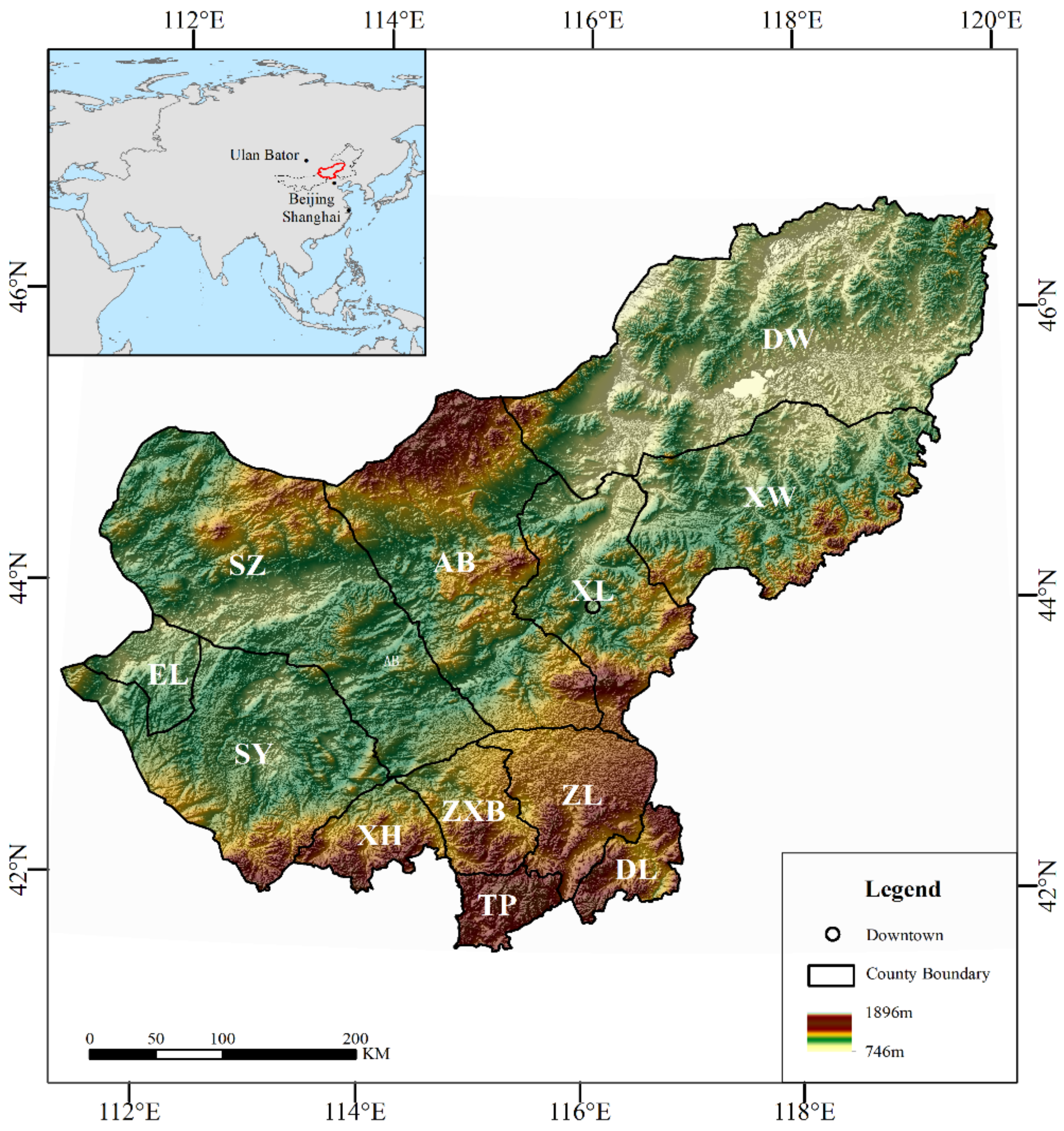
2.1. Study Area

Xilingol, a typical zone of arid and semi-arid grassland in Northern China (43–44°N, 115–117°E), is located in the southeastern edge of the Mongolian Plateau, and in the central part of the Inner Mongolia Autonomous Region of China, with a total area of 20.3 × 10⁴ km2 (Figure 1). Located in the middle temperate zone, the study area has arid and semi-arid continental monsoon climate, which is characterized by aridity, low rainfall, and high winds, with spatial variability in temperature in the form of a north–south gradient. The mean annual temperature is 1–4 °C, and the annual precipitation is 150–400 mm, with 70% of the annual precipitation concentrated between June and September; the evaporation is between 1500–2700 mm [31].
The general landscape of the Xilingol region consists of gently undulating hills, plateaus, and dunes; the elevation gradually decreases from south to north, with an average altitude of 800–1800 m; it is bordered by the northern foothills of Yin Mountain in the south and the Gobi of the Mongolian Plateau in the north; it is a zone of transition from the arid northwest to the humid east and a sensitive area in responding to global change [33].
From east to west, across the Xilingol grassland region, precipitation and soil fertility decrease gradually, creating three separate vegetation types: meadow steppe, typical steppe, and desert steppe, which are commonly referred to as the zonal vegetation types in Chinese literature. In addition, there are also a few “non-zonal” vegetation regions in the study area, including shrublands, woodland, saline meadows, and lowland marshes [35].

2.2. Data Description

Various satellite images and geographic, environmental background datasets were used in the study (Table 1), comprising all Landsat 5/7/8 images and EVI/NDVI/NDWI products of the Xilingol during the summer, as well as SRTM V3, global night-time light products, and China’s land-use/cover datasets (CLUDs). To investigate the driving forces of LULC, the climatic data and regional socioeconomic statistical yearbook data were also selected. All of the base datasets were integrated into the GEE platform and can be used directly, except for CLUDs and regional socioeconomic statistical yearbook data.
Landsat 5/7 images we used include bands 1 (0.45–0.53 μm), 2 (0.52–0.60 μm), 3 (0.63–0.69 μm), 4 (0.76–0.90 μm), 5 (1.55–1.75 μm), and 7 (2.08–2.35 μm), and Landsat 8 images include bands 1 (0.43–0.45 μm), 2 (0.45–0.51 μm), 3 (0.53–0.59 μm), 4 (0.64–0.67 μm), 5 (0.85–0.88 μm), 6 (1.57–1.65 μm), 7 (2.11–2.29 μm), 10 (10.6–11.19 μm), and 11 (11.50–12.51 μm). EVI/NDVI/NDWI products are derived from Landsat 5/7/8 Collection 8-Day composites [36]. The EVI/NDVI indices were introduced to improve the classification accuracy of grassland and woodland [37], and the NDWI index was introduced to improve the classification accuracy of lakes and rivers [38].
SRTM V3 data (Shuttle Radar Topography Mission Version 3) are from NASA JPL, providing a near-global scale digital elevation model [39]. The SRTM V3 product was introduced to eliminate the impact of mountains.
Night-time lights products include the DMSP-OLS Nighttime Lights Time Series product from the Defense Meteorological Satellite Program (DMSP) and the NPP-VIIRS Day/Night Band (DNB) product from the Suomi National Polar-orbiting Partnership. Both products can detect visible and near-infrared emissions in cities and towns, using sensors that can capture low-light emission sources under varying illumination conditions, resulting in an effective improvement in the classification accuracy of built-up areas.
To construct highly reliable training and validation sample sets for RF models quickly and efficiently, as well as to reduce the huge labor and time costs associated with visual interpretation, Hu et al. proposed a computer-automated selection of the samples based on the principles of “multi-source consistency” and “time-series stability” [40,41]. This method was applied in our study to extract areas with no change in land-use types based on the five land-use datasets of 2000, 2005, 2010, and 2015 of the 30 m China’s land-use/cover datasets (CLUDs), which were provided by the Institute of Geographical Sciences and Resources of the Chinese Academy of Sciences, and then generated sample sets. The classification system we adopted was proposed by Liu et al. [42]; this classification used a two-level structure to group land-use types into 6 major classes and 25 sub-classes, which has been widely used in Chinese academia and government planning. In the study, the main land-use type in Xilingol is grassland, to describe the differences within grassland more carefully, we further subdivided the grassland into secondary classes (i.e., high-coverage grass, moderate-coverage grass, and low-coverage grass) according to the differences of grassland coverage, forming a classification system of 8 categories of LULC.
The climatic data, namely, precipitation, temperature, and climate water deficit, were separately derived from PERSIANN-CDR [43], GLDAS-2.1 [44] and TerraClimate [45] datasets. The data of total precipitation and mean temperature in the summer and mean growing season climate water deficit data were further obtained based on the original data.
The data from the regional socioeconomic statistical yearbook were divided into 7 categories in the study: population and labor force, regional economic development, industrial structure, agricultural and pastoral production, agricultural and pastoral input, and residential income. All the indicator data (2000–2020) were obtained from literature, including “Xilingol League Statistical Yearbook”, “Inner Mongolia Statistical Yearbook”, “China Population, and Employment Statistical Yearbook”, “Inner Mongolia in 30 Years of Reform and Opening Up”, “China Regional Economic Statistical Yearbook”, “60 Years of Glory”, etc. The specific indicator items are listed in Table 2. All the above data are included in the China Economic and Social Big Data Research Platform (https://data.cnki.net/NewHome/index, accessed on 15 November 2021).

3. Land-Use Mapping Methods

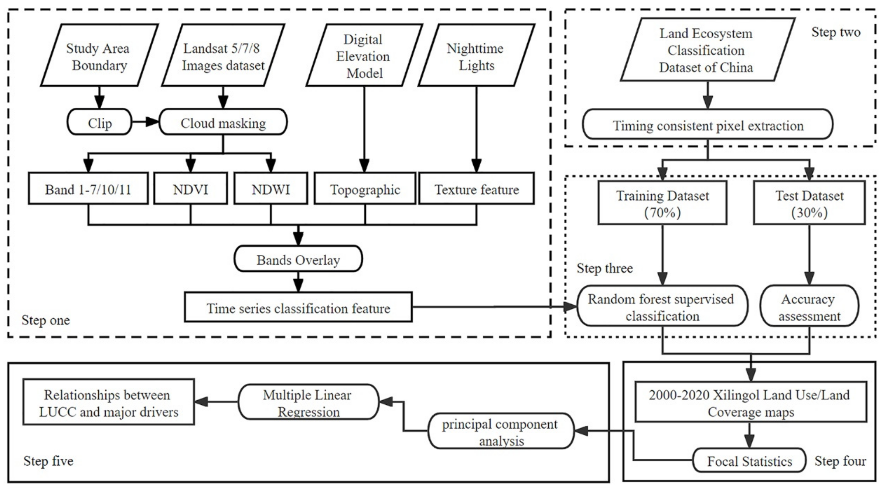
3.1. Technical Process

The overall land-use mapping technical process is illustrated in Figure 2 and comprises the following four steps:
  • Based on the Landsat images and EVI/NDVI/NDWI indices and night-time light data, together with other related auxiliary data in GEE, we used image synthesis and cloud mask methods to extract the 2000–2020 composite images without cloud or shadow coverage in Xilingol.
  • Based on the principle of “time-series stability” of the corresponding image attributes in the multi-period CLUDs, we selected sample points with no change in land-use type in the CLUDs to form the sample points set required for the RF model.
  • Setting 70% of the sample points as training sample points, combined with the synthetic images, RF model training was carried out to interpret the LULC dataset of each year. The remaining 30% of the sample points were used as validation sample points to evaluate the accuracy of classification results.
  • Supported by the climate change and regional socioeconomic development factors, principal component analysis was applied to determine the categories of LULC drivers; then, the contribution of each driving factor was calculated by multiple stepwise regression method.

3.2. LULC Dataset Production

With the support of the GEE platform, the image synthesis and cloud mask methods were applied to produce cloud-free composite images for each year in the summer [46]. Specifically, to eliminate image quality problems caused by cloudy and rainy areas in the Xilingol, we replaced and supplemented low-quality pixels of each year with the previous and following year’s TOA reflectance data to produce the best available pixel image composites. Based on the image cloud distribution probability score, we selected the images with less than 30% cloud coverage. Then, a median composite method was applied to combine collection into a single image [41], resulting in the annual cloud-free image dataset in summer from 2000 to 2020.

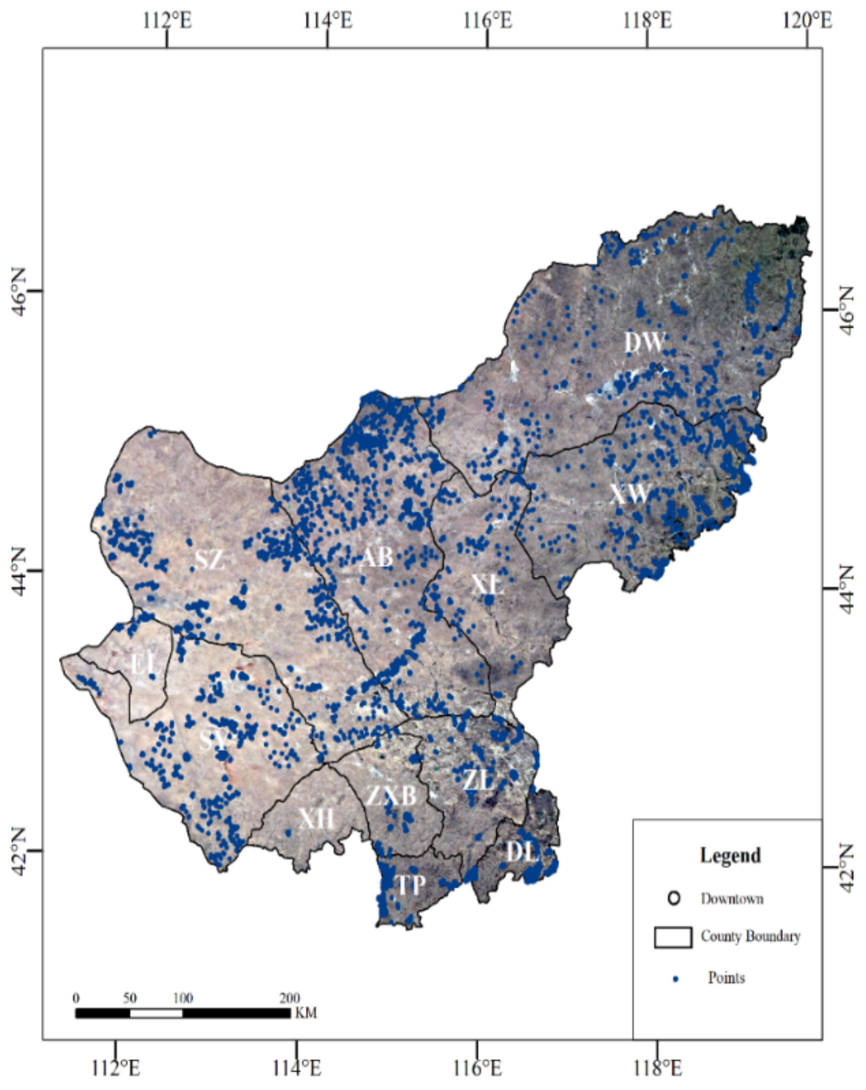
3.3. Sample Points Set Deployment

Supervised classification commonly requires many training samples and validation samples. In traditional studies, the method of manual visual interpretation is generally used to obtain sample points. However, for such a large area as Xilingol, it will take a lot of labor and time to obtain sufficient samples by relying on the manual visual interpretation method. Based on the “time-series stability” principle, a highly reliable and automated sample point selection method was achieved in the study by selecting pixels with “identical” attributes from multi-period LULC products [40]. The specific steps are:
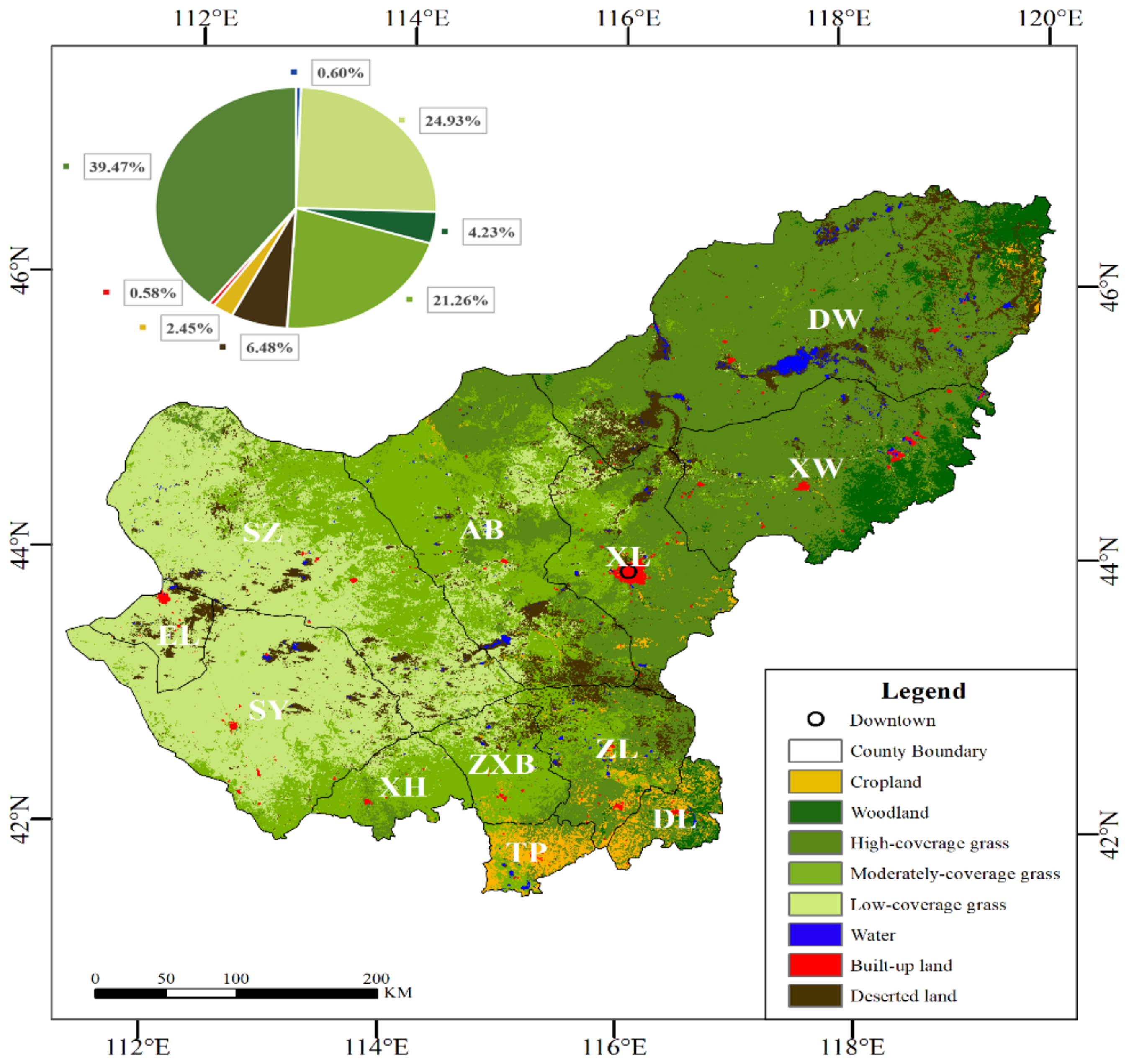
  • Unified classification system. Reclassification of land-use types in Xilingol into eight categories: cropland, woodland, high-coverage grass, moderate-coverage grass, low-coverage grass, water, built-up land, and deserted land (Table 3).
  • Selection of image pixels. We overlapped the CLUDs of 2000, 2005, 2010, and 2015 in the study area to obtain the pixels with no change in land-use types during this period.
  • Stratified random sampling. To avoid the risk of sample bias (excessive representation of correct or incorrect points), a stratified random sampling method was adopted to randomly deploy sample points in the above target pixels regarding the area composition proportion of various land-use types. In this study, a total of 4800 samples were deployed.
  • Manual adjustment of position. Based on the sample points mentioned above, the high-resolution (10 m) satellite images Sentinel-2A were used to remove the sample points, which were too close to the boundary of the plot, and retain those located in the central part of the plot. In this study, 4788 samples were finally formed.

3.4. Random Forest Method

The RF classifier is an ensemble classifier that uses a set of decision trees to make a prediction and applies a voting mechanism to the results [20]. Specifically, each decision tree is judged independently, and each node is split using a user-defined number of features. The final classification decision is made by averaging the probabilities of class assignment calculated by all generated trees, and the class with the maximum votes is the final class chosen [47]. RF allows the training and classification process to be highly parallelized and run efficiently despite the high dimensionality of the sample features, thus improving the overall predictive performance of the model and reducing the phenomenon of overfitting [48]. To balance operational efficiency and accuracy of operational results, this study set the number of decision trees in the random forest to 200 after iterative trials. The analysis and implications of the size of the number of decision trees in the random forest can be found in the Discussion section of this paper (Section 4.1).

3.5. Accuracy Assessment of Results

To evaluate the sample points’ set construction method under the principle of “time-series stability” and confirm whether the above method is competent for automated, long time-series, and high-precision land-use mapping tasks, based on the method proposed by Olofsson [49], we calculated the overall accuracy, kappa coefficient, user accuracy (UA), and producer accuracy (PA) of the clarification results for each year by constructing the confusion matrix. The confusion matrix represents the relationship between known reference data (true land-use type) and the corresponding results of the classification process on each land-use type. User accuracy represents the frequency with which the classifications on the map will appear on the ground, and producer accuracy represents the proportion of the total observations that are correctly judged for each classification on the map.

3.6. Analysis of Driving Mechanisms

In this study, we proposed a “two-step” analytical framework. The first step is to carry out a principal component analysis of all factors recognized in the general LULC analysis, i.e., meteorological factors, socioeconomic development factors, industrial structure factors, and cost and benefit factors, to simplify the complex changes into a few key dimensions; subsequently, selecting the primary factors within the key dimensions and carrying out stepwise regression modeling based on the relationship between typical LULC and key elements. Through the above two steps, we finally achieved the objective of accurately identifying the driving factors and determining their contribution.

3.7. Principal Components Analysis

Principal component analysis (PCA) is an important dataset-simplification method in multivariate statistical analysis. With a core idea of reducing the dimension of variables while preserving the information of variables as much as possible, the PCA method performs orthogonal transformation on the observed values of a series of possibly related variables and re-projects the observed values of these variables into the values of a series of linearly unrelated variables, which are called principal components. Moreover, these new variables are in order, and the first few variables retain most of the changes in the original variables [50]. Here, principal component analysis was adopted to concentrate the change information of all 19 indicators (Table 2) into multiple principal components.
From a mathematical point of view, assuming that x has n samples and each sample has p variables, the matrix of order n × p is formed:
X = x 11 x 12 x 1 p x 21 x 22 x 2 p x n 1 x n 2 x n p
We performed linear transformation on this variable, and the comprehensive indexes are, respectively: z 1 , z 2 , , z m ,   m p
z 1 = l 11 x 1 + l 12 x 2 + + l 1 p x p z 2 = l 21 x 1 + l 22 x 2 + + l 2 p x p z m = l m 1 x 1 + l m 2 x 2 + + l m p x p
In the formula, the coefficient l i j   is determined by the following principle:
(1) z i is independent of z j ; (2) z 1 is the largest variance among all linear combinations, and z m is the smallest variance among all linear combinations. At this point, the new variables z 1 , z 2 , z 3 are the first, second, and third principal components of the original variables, respectively. In practical problems, the first few largest principal components are often chosen to simplify the relationship between variables.

3.8. Multiple Linear Stepwise Regression Analysis

Multiple stepwise regression analysis is a method of fitting a regression model. For a given set of predictor variables, the model is repeatedly regression-analyzed and significance-tested through an automated procedure, and a set of explanatory variables is considered for addition or deletion based on some pre-defined criteria, ultimately retaining only those explanatory variables that significantly improve the model. The multiple regression model is as follows:
Y = β + α 1 X 1 + α 2 X 2 + + α n X n
where α 1 , α 2 , , α n   represent the correlation coefficients, and β is a constant term.
The PCA was completed with the support of SPSS [51], and the multiple linear stepwise regression analysis was completed with the support of R [52]. All the GEE JavaScript code and driving forces analysis data involved in the study are uploaded as Supplementary Materials.

4. Results

4.1. Selection of Sample Points

The main land-use type in Xilingol is grassland, while the other land-use types are small and scattered. Therefore, the sample points of grassland are generally distributed evenly, while the sample points of other land-use types (e.g., built-up land and water) show a dense distribution (Figure 3).

4.2. Accuracy Assessment of Classification Results

With the support of GEE, we obtained a LULC dataset (30 m) for Xilingol for 2000–2020. The overall accuracy of this dataset was 0.88 ± 0.01, and the Kappa coefficient was 0.87 ± 0.02 (Table 4). The averaged results of user accuracy and producer accuracy of all land-use types in 21 years (Table 5) show that user accuracy and producer accuracy of built-up land and water are relatively high (0.99 ± 0.01, 0.99 ± 0.01; 0.98 ± 0.01, 0.94 ± 0.02) while high- and moderate-coverage grass are comparatively low (0.80 ± 0.03, 0.85 ± 0.03; 0.80 ± 0.03, 0.78 ± 0.04).
The high accuracy of built-up land and water classification is related to the full application of night-lighting products and NDWI auxiliary data. The low accuracy of high-coverage grass is mainly due to more misclassifications between high- and moderate-coverage grass. The low accuracy of moderate-coverage grass is mainly due to more misclassifications and omissions between this category and high-and low-coverage grass (Table 6).

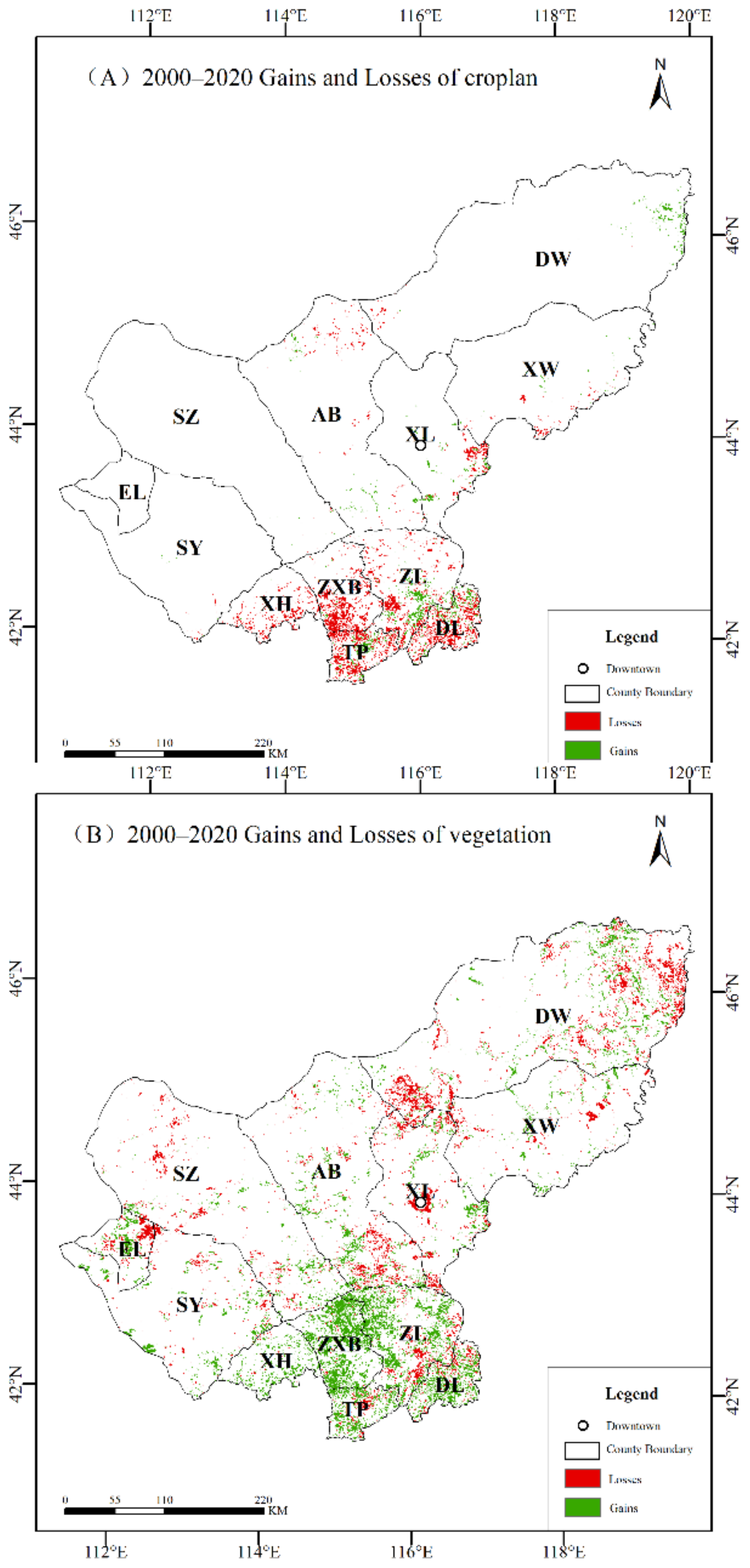
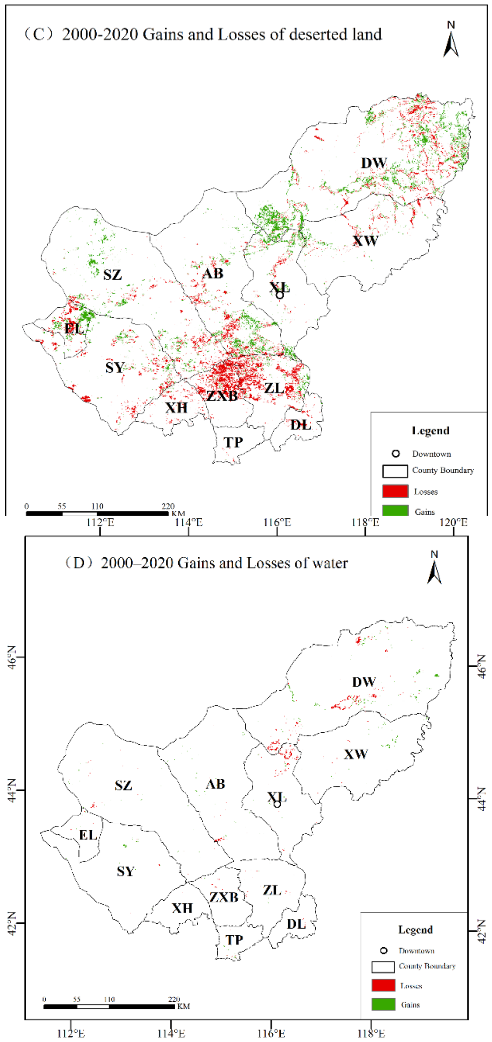
4.3. Spatial Pattern of LULC

Grassland, which accounted for more than 85.6% of the total area in 2020, was the main land-use type in Xilingol. Specifically, the area of high-coverage grass was the largest, followed by low-coverage grass, and the area of moderate-coverage grass was the smallest, with the area of grassland ranging from 24% to 39% of the total area. The area of the other three land-use types, namely deserted land, woodland, and cropland, decreased in order, accounting for 2–6% of the total area, while the area of water and built-up land was the smallest, covering only 0.6% and 0.58% of the total area (Figure 4).
The basic spatial patterns of LULC in Xilingol in 2020 can be summarized as follows.
The grassland area decreased from the east to the west. High-coverage grass was primarily distributed in the east (Dongwuzhumuqin, Xiwuzhumuqin, and Xilinhot); moderate-coverage grass was mainly distributed in the center and south (Abaga, Xilinhot, eastern part of Sunitezuo, Zhengxiangbai, Xianghuang, and Zhenglan); low-coverage grass was primarily distributed in the center and west (Sunitezuo, Suniteyou, Erlianhot, northern part of Zhengxiangbai and Abaga). Woodland was mainly distributed in the east of the greater Khingan Mountains (Dongwuzhumuqin and Xiwuzhumuqin); cropland was mainly in the south and southeast (Taipusi, Duolun, Zhenglan, and Xilinhot) and in the urban periphery, usually forming agro-pastoral ecotone together with grassland. Water was mainly located in the east and center (Ulagai water system in the northeast, and Hurchagannuoer water system in the middle). Deserted land was mainly located in the core area of the Hunshandake Sandy Land (northern part of Zhenglan, northern part of Zhengxiangbai, central and northern part of Sunitezuo, central and northern part of Suniteyou and Erlianhot), in the Gobi area of the Mongolian Plateau in the northwest, and at the periphery of the lake and river in the northeast. Built-up land was sporadically distributed throughout the study area.

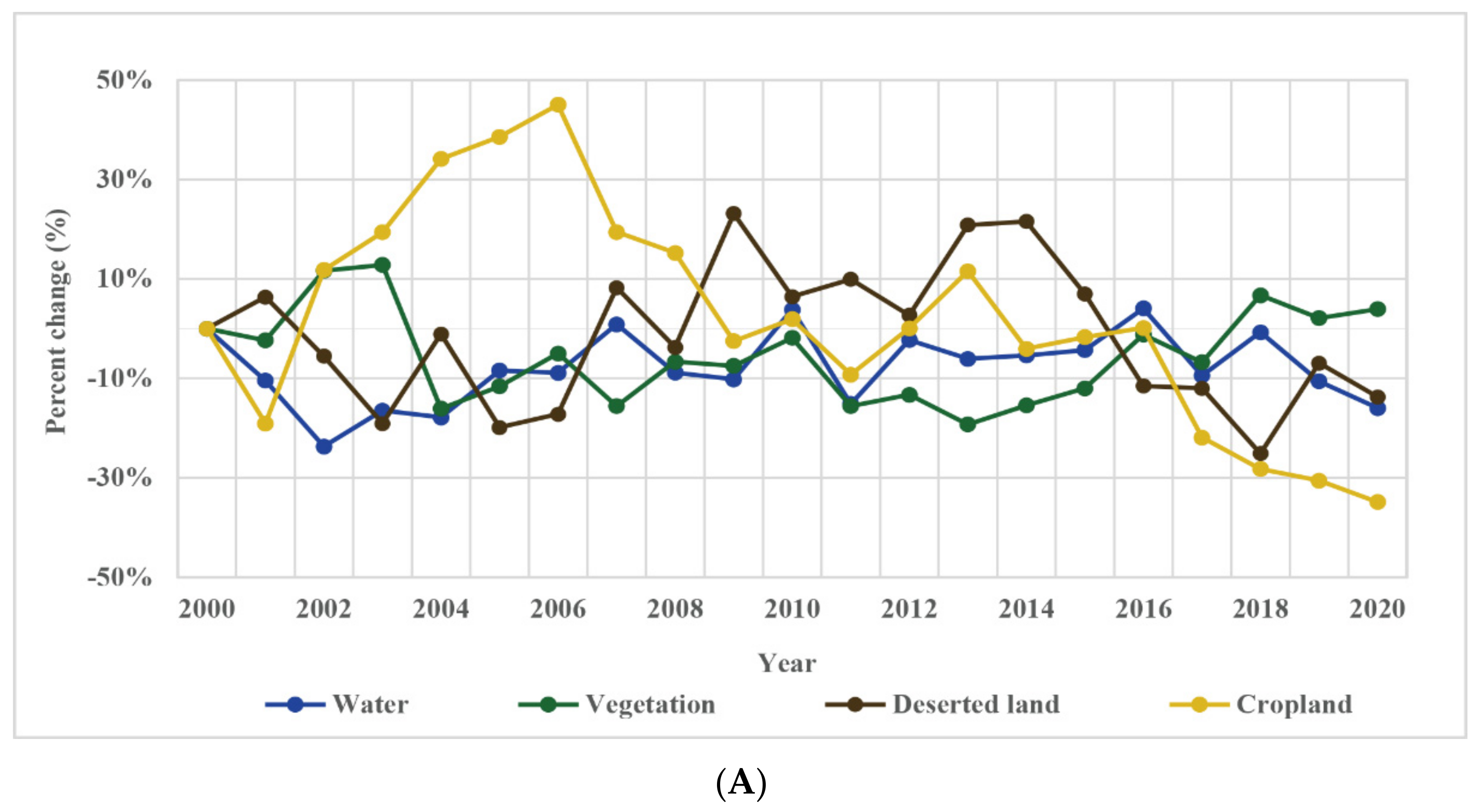
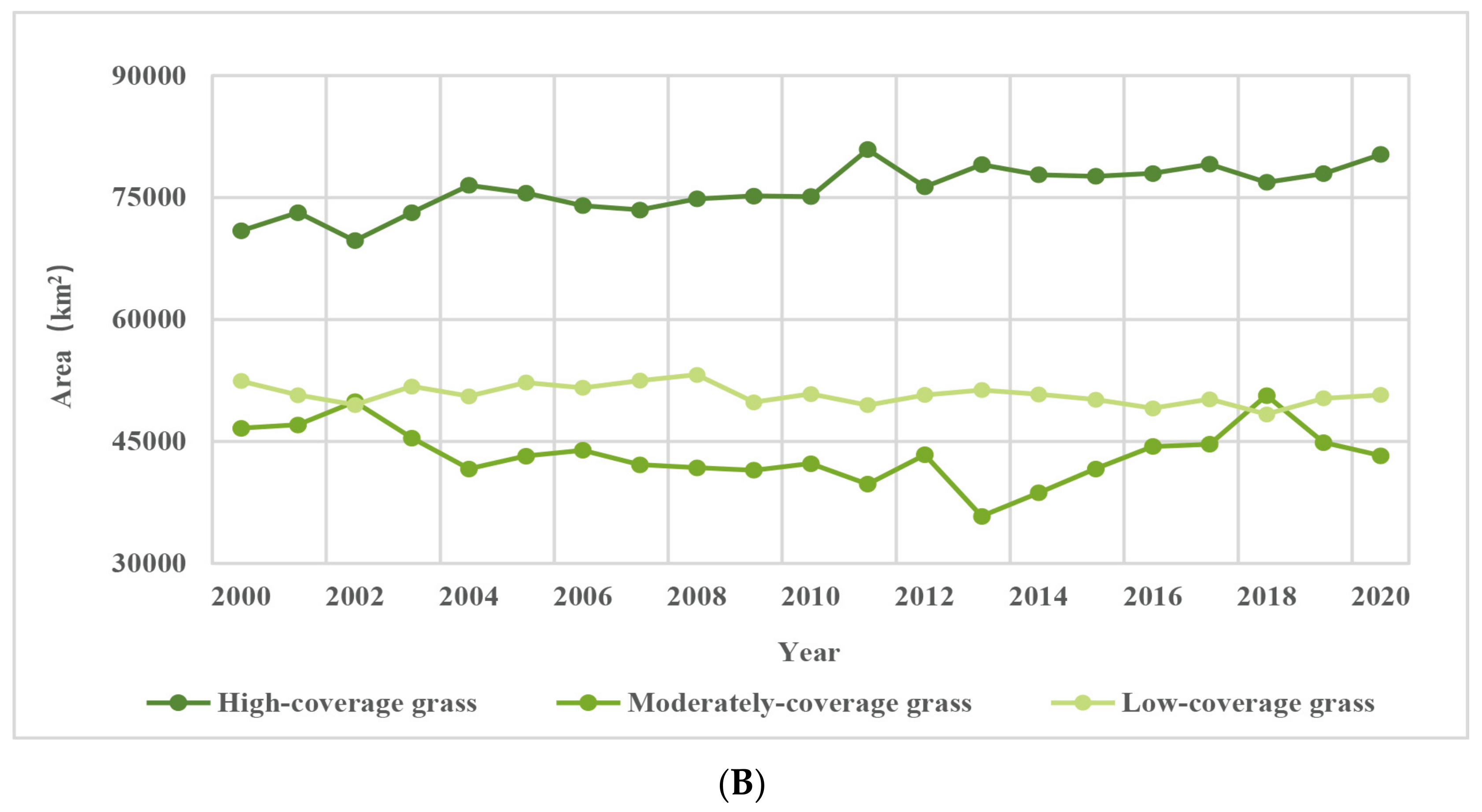
4.4. Temporal Characteristics of LULC

From 2000 to 2020, the ecological status in Xilingol indicated significant characteristics of improvement. In particular, the area of natural vegetation (grassland and woodland) increased slightly (+4.42 × 10³ km2, +3.95%), but the area of deserted land, water, and cropland presented a shrinking trend (Figure 5A). Of the natural vegetation, high-coverage grass continued increasing; moderate-coverage grass decreased first and then increased, but the total area remained decreased; low-coverage grass gradually decreased (Figure 5B).
From 2000 to 2020, the basic temporal characteristics of changes in various land-use types in Xilingol can be summarized as follows.
Overall, cropland lost amounted to 4.51 × 10³ km2, which was mainly used for natural vegetation and built-up land, mainly due to the implementation of the “Grain for Green” Project and the expansion of built-up land (Table 7). During the same period, cropland gained 1.49 × 10³ km2, mainly from natural vegetation and deserted land, but the total cropland showed conversion and abandonment. The decreased cropland is concentrated in the agro-pastoral ecotone of south Xilingol (Zhenglan, Zhengxiangbai, Xianghuang, Taipusi, and Duolun) (Figure 6A).
During the two decades, natural vegetation lost totaled 7.68 × 10³ km2, which was mainly converted to cropland and deserted land (Table 7). Meanwhile, natural vegetation gained 1.22 × 10⁴ km2, mainly from cropland and deserted land, with increased natural vegetation mainly in the south and west Xilingol due to expansion of low-coverage grass into high- and moderate-coverage grass (Zhenglan, Zhengxiangbai, Xianghuang, Taipusi, and Duolun). Although the natural vegetation in the entire region gradually increased, in individual banners and counties (e.g., Dongwuzhumqin and Sunitezuo), the natural vegetation showed a shrinking trend (Figure 6B).
In addition, deserted land lost 7.85 × 10³ km2 and was mainly used for natural vegetation; an obvious change was concentrated in the Otindag Sandy Land (Zhengxiangbai and Zhenglan) of the center, which indicated that the land desertification has been significantly restrained and presented a greening trend (Table 7). During the same period, deserted land gained 5.90 × 10³ km2, mainly from natural vegetation and water, and increased deserted land was mainly concentrated in the Dongwuzhumuqin of the northeast, mainly due to the obvious land salinization process caused by the drying up of rivers and lakes (Figure 6C).
During the same period, water lost amounted to 6.16 × 10² km2 and was mainly converted to deserted land and grassland (Table 7); decreased water was mainly concentrated in the major water system of Dongwuzhumuqin due to the shrinking of rivers and the drying up of lakes, as well as the recovery of grassland. Meanwhile, water gained amounted to 3.57 × 10² km2, mainly from deserted land and grassland (Figure 6D).

4.5. Driving Forces and Driving Mechanisms of LULC

Using PCA, the information on the changes of all 19 indicators (Table 2) can be concentrated on three principal components (Table 8). Among them, the first principal component (F1) is a characterization of the regional socioeconomic development and agricultural construction condition, mainly including the gross domestic product (X7), rural electricity consumption (X15), the total power of agricultural machinery (X16), and gross agricultural product (X8); the second principal component (F2) is a characterization of the climate, mainly including the mean growing season climate water deficit (X3), total summer precipitation (X1), and mean summer temperature (X2); the third principal component (F3) is a characterization of the development of the grassland livestock industry, mainly the total number of livestock (X13).
Using various land-use types area as the dependent variables and the above principal components as the independent variables, the regression models of typical land-use types can be obtained by applying the multiple linear stepwise regression method; their significance level and R2 are shown in Table 9. The results showed that regional economic development and agricultural construction factor (F1) have a significant positive impact on the area of cropland. In addition, the grassland area was negatively correlated with economic development and agricultural construction factor (F1) and positively correlated with animal husbandry factor (F3). The water area has a positive relationship with regional socioeconomic development and agricultural construction factor (F1) and climate factor (F2). It should be noted that the regression models for grassland and water have not passed the significance test.
Furthermore, we used land-use type areas as the dependent variables and the following key factors as input variables: X7, X8, X15, and X16 in F1 (absolute values of factor information loadings above 0.98 in the rotated component matrix); X1, X2, and X3 in F2 (absolute values of factor information loadings above 0.70 in the rotated component matrix); and X13 in F3 (absolute values of factor information loadings above 0.65 in the rotated component matrix) to fit the multiple linear regression models of typical land-use types (Table 10). In general, built-up land (Y4) has a highly significant positive correlation with the gross domestic product (X7), primarily due to the promotion of urban expansion by the regional economic development. The area of water (Y3) positively correlates with the mean summer temperature (X2), which is mainly due to the continuous warm climate. There is no statistically significant relationship between the area of cropland and grassland and other relevant factors.

5. Discussion

5.1. Land-Use Mapping Methods

The GEE platform greatly reduced the time and cost required for researchers to find and process the fundamental data [53]. In the study, we created a LULC dataset in Xilingol by retrieving 2436 satellite images during 2000–2020. The sample database construction method [40] can complete the entire land-use mapping task quickly and accurately in only 18,900 s by applying the principle of “time-series stability” and combining with the land classification method of random forest. The study shows that using the RF algorithm for LULC in Xilingol leads to better results. By comparing different machine-learning methods, the validity of the RF classifier has also been verified in other land-use classification studies [19].
According to the principle of parsimony, the RF parameters were optimized to balance model complexity (size of the RF classifier) and classifier performance [54]. We found that RF exhibited signs of overfitting (large difference between training and validation error) if the complexity of RF was not constrained. Limiting the number of decision trees can reduce the complexity of the model and narrow the gap between training and validation errors [55]. The classification results also showed that reducing the number of decision trees (from 120 to 40) resulted in a loss of approximately 1–2% in validation accuracy, which was recovered by increasing the number of decision trees.
We used the “compare after classification” approach for LULC monitoring. In contrast to the continuous change-detection algorithms (e.g., CCDC, LandTrendr, CVAPS-NDVI, etc.) [56,57,58], this method has a significant shortcoming which ignores the temporal continuity of land-use changes at the same pixel during adjacent years, which might treat algorithmic classification errors as real type changes. In addition, the mapping accuracy of high- and moderate-coverage grass are both low, mainly due to the fact that moderate-coverage grass is a transition type between high- and low-coverage grass (Table 5 and Table 6); meanwhile, in the southern agro-pastoral ecotone, cropland is scattered within the grassland, which also caused low mapping accuracy of grassland (Table 5 and Table 6).
In addition, the pixel-based LULC classification method we used only takes spectral features as input variables for discrimination features, and several studies showed that an object-oriented discrimination method based on clustering and segmentation could combine spectral and geometric information with the texture information from high-resolution images to effectively improve the accuracy of LULC classification in urban and vegetation areas [59,60,61]. In subsequent studies, we can apply high-resolution images combined with methods such as continuous change-detection algorithms and object-oriented discrimination methods to produce higher-accuracy LULC classification results.

5.2. Spatial Patterns and Characteristics of LULC

In this study, we produce an annual LULC dataset for 2000–2020 in Xilingol, and the results indicate that the ecological state of the study area improves significantly [35,62], with the area of natural vegetation expanding steadily, especially high-coverage grass. The results are generally consistent with the findings by Zhao et al. and Wang et al. Zhao et al. showed an overall improvement in grassland quality in Xilingol during 2000–2013 [34]. Wang et al. found that the direction of shift in grassland coverage during 2000–2008 for different classes is mainly towards higher classes [63]. Our study suggests that during 2000–2020, high-coverage grass increases by 13.26%, moderate-coverage grass decreases by 7.23%, and low-coverage grass decreases by 3.27%. Compared to previous studies, our findings reveal the dynamics of changes over a longer time scale (2000–2020) and across a wider range of land-use types. Moreover, our study indicates that the area of cropland, water, and deserted land is gradually shrinking, and build-up land is rapidly expanding. The results are consistent with the findings of Batunacun et al. They found four land-use change processes in Xilingol during 2000–2015, i.e., expansion of built-up land, restriction of cropland expansion, increase in grassland, and decrease in water [32].
The LULC dataset obtained in this study is largely consistent with the GlobeLand30 in terms of the general land-use pattern, and our dataset is more suitable for the characteristics of land classification in Xilingol. As grassland is the dominant land-use type in Xilingol, we have classified grassland into three categories based on the coverage, whereas GlobeLand30 has only one category [64,65]. Following a comparative analysis of five typical land-use categories in Xilingol (cropland, grassland, woodland, built-up land, water, and deserted land), it was found that 77.23% of the pixels in the 2000 product from this study are consistent with the GlobeLand30 product; 82.2% of the pixels in the 2020 product are consistent with the GlobeLand30 product (mainly grassland and built-up land). The main difference between two datasets is the discrimination of land-use types in some transition areas (mainly cropland and deserted land).

5.3. Uncertainty in the Analysis of Driving Mechanisms

In the study, PCA was used to classify the variables that might affect LULC. Subsequently, the key factors were extracted from each group and the stepwise method was used to fit the multiple linear regression model. In particular, among all the linear regression models fitted in Table 10, not all the input variables and dependent variables have a cause-and-effect relationship. Although this study provides a method for extracting key variables from various potential variables hierarchically, identifying the drivers, and fitting the regression models, the completeness of selected independent variables and whether these variables can truly and effectively reflect the driving mechanisms of land-use change have great impacts on the reliability of the results [66]. In addition, although we retained independent explanatory variables when possible, potential multicollinearity between the drivers was not quantified and fully removed before the regression analysis, which may cause model instability and increase the complexity of interpretation of results [67].
The overall results of the driving mechanism we obtained are consistent with previous studies, but there are still some differences. Xu et al. suggested that the mean annual precipitation and distance to the nearest settlement were closely related to LULC [33]. Hu et al. concluded that climate change had an important impact on the evolution of the Xilingol ecosystem, and the effects of human activities superimposed on climate change may accelerate the evolution of the ecosystem [68]. Shi et al. suggested that the heterogeneity of spatial changes in vegetation was mainly influenced by both climate and human activities [69]. Our results reveal that, except for two specific relationships (i.e., national economic development facilitating the expansion of built-up land, warming climate facilitating the increase of water), which can be statistically confirmed, the other land-use types (cultivated land, grassland) have no significant relationship with relevant variables. This is probably because the study region is part of the agro-pastoral transitional zone, where changes of cropland and grassland might indeed be largely edaphically or climatically determined. More generally, in response to the interaction of human activities and environmental drivers, the ecosystems of cropland and grassland are both highly dynamic and also resilient, with some patches moving through multiple vegetation types, resulting in disorderly patterns of transformation.

6. Conclusions

LULC is the most direct manifestation of the interaction between human activity and the natural environment. Spatial patterns and characteristics of LULC can reflect the intensity and modes of human–environment interactions. We generated a yearly updated LULC dataset in Xilingol from 2000 to 2020 using random forest algorithm in the GEE platform, along with high-resolution satellite remote-sensing images. Based on the dataset, we investigated the spatiotemporal characteristics, dynamic changes, and driving mechanisms of LULC. Given the convenience of the GEE platform for remote-sensing analysis and the importance of the RF algorithm in automated classification studies, the technical process and modeling approach used in this study are of great reference value for conducting similar studies in other regions in the future. The application of continuous change-detection algorithms and object-oriented discrimination methods to land-use change is our further research direction.
Our results suggest that, during the two decades between 2000 and 2020, the ecological status across Xilingol indicates significant improvement characteristics. The area of high-coverage grass and woodland increases while the area of water and moderate- and low-coverage grass decreases. Cropland increases first and then decreases, which is mainly distributed in the southeast. The area of deserted land decreases in the south and increases in the center and north, but the total area still decreases. The built-up land expands rapidly. In addition, our results suggest that regional socioeconomic development factors are the primary causes of changes in built-up land, and climate-related factors drive variations in the spatial pattern of water. This study is helpful not only to reveal the dynamics of LULC in Xilingol since the large-scale implementation of the “Beijing–Tianjin Sandstorm Source Control” project but also to better understand the mechanisms contributing to LULC in the context of global climate change and regional socioeconomic development and to further achieve intensive and sustainable development of the regional agriculture and animal husbandry.

Supplementary Materials

Provided. The availability of the GEE JavaScript code of stratified sample points set is as follows: https://code.earthengine.google.com/32498ad3ddf57a8ff715c86da9f77e8e (accessed on 15 November 2021); the availability of GEE JavaScript code of RF method for supervised classification is as follows: https://code.earthengine.google.com/722a682b42110a80fa9adfc36653d16a (accessed on 15 November 2021); The availability of driving forces analysis dataset uploaded as a CSV file.

Author Contributions

Acquisition, Y.H.; Investigation, J.Y.; Methodology, Y.H. and J.Y.; Validation, J.Y., Y.H. and L.Z.; Visualization, J.Y. and Y.H.; Writing—original draft, J.Y.; Writing—review and editing, Y.H., L.Z., H.W. and Y.Z. All authors have read and agreed to the published version of the manuscript.

Funding

This work was funded by the National Natural Science Foundation of China (41977421, 42130505), and the Strategic Priority Research Program of the Chinese Academy of Sciences [XDA19040301, XDA20010202, XDA23100200].

Institutional Review Board Statement

Not applicable.

Informed Consent Statement

Not applicable.

Data Availability Statement

Not applicable.

Conflicts of Interest

The authors declare no conflict of interest.

References

  1. Mooney, H.A.; Duraiappah, A.; Larigauderie, A. Evolution of natural and social science interactions in global change research programs. Proc. Natl. Acad. Sci. USA 2013, 110, 3665–3672. [Google Scholar] [CrossRef] [PubMed] [Green Version]
  2. Chen, C.; Park, T.; Wang, X.; Piao, S.; Xu, B.; Chaturvedi, R.K.; Fuchs, R.; Brovkin, V.; Ciais, P.; Fensholt, R.; et al. China and India lead in greening of the world through land-use management. Nat. Sustain. 2019, 2, 122–129. [Google Scholar] [CrossRef] [PubMed]
  3. Geist, H.J.; Lambin, E.F. Proximate Causes and Underlying Driving Forces of Tropical DeforestationTropical forests are disappearing as the result of many pressures, both local and regional, acting in various combinations in different geographical locations. Bioscience 2002, 52, 143–150. [Google Scholar] [CrossRef]
  4. Liu, J.; Kuang, W.; Zhang, Z.; Xu, X.; Qin, Y.; Ning, J.; Zhou, W.; Zhang, S.; Li, R.; Yan, C.; et al. Spatiotemporal characteristics, patterns, and causes of land-use changes in China since the late 1980s. J. Geogr. Sci. 2014, 24, 195–210. [Google Scholar] [CrossRef]
  5. Overmars, K.P.; Verburg, P. Analysis of land use drivers at the watershed and household level: Linking two paradigms at the Philippine forest fringe. Int. J. Geogr. Inf. Sci. 2005, 19, 125–152. [Google Scholar] [CrossRef]
  6. Liu, X.; Liang, X.; Li, X.; Xu, X.; Ou, J.; Chen, Y.; Li, S.; Wang, S.; Pei, F. A future land use simulation model (FLUS) for simulating multiple land use scenarios by coupling human and natural effects. Landsc. Urban Plan. 2017, 168, 94–116. [Google Scholar] [CrossRef]
  7. Zhang, J.-T.; Ru, W.; Li, B. Relationships between vegetation and climate on the Loess Plateau in China. Folia Geobot. Phytotaxon. 2006, 41, 151–163. [Google Scholar] [CrossRef]
  8. Naikoo, M.W.; Rihan, M.; Ishtiaque, M. Shahfahad Analyses of land use land cover (LULC) change and built-up expansion in the suburb of a metropolitan city: Spatio-temporal analysis of Delhi NCR using landsat datasets. J. Urban Manag. 2020, 9, 347–359. [Google Scholar] [CrossRef]
  9. Foley, J.A.; DeFries, R.; Asner, G.P.; Barford, C.; Bonan, G.; Carpenter, S.R.; Stusrt Chapin, F.; Coe, M.T.; Daily, G.C.; Gibbs, H.K.; et al. Global consequences of land use. Science 2005, 309, 570–574. [Google Scholar] [CrossRef] [Green Version]
  10. Yao, Z.; Wang, B.; Huang, J.; Zhang, Y.; Yang, J.; Deng, R.; Yang, Q. Analysis of Land Use Changes and Driving Forces in the Yanhe River Basin from 1980 to 2015. J. Sens. 2021, 2021, 6692333. [Google Scholar] [CrossRef]
  11. Schroeter, D.; Cramer, W.; Leemans, R.; Prentice, I.C.; Araújo, M.B.; Arnell, N.W.; Bondeau, A.; Bugmann, H.; Carter, T.R.; Gracia, C.A.; et al. Ecosystem Service Supply and Vulnerability to Global Change in Europe. Science 2005, 310, 1333–1337. [Google Scholar] [CrossRef] [Green Version]
  12. Wang, Y.; Shao, M.; Zhu, Y.; Liu, Z. Impacts of land use and plant characteristics on dried soil layers in different climatic regions on the Loess Plateau of China. Agric. For. Meteorol. 2011, 151, 437–448. [Google Scholar] [CrossRef]
  13. Jetz, W.; Wilcove, D.S.; Dobson, A.P. Projected Impacts of Climate and Land-Use Change on the Global Diversity of Birds. PLoS Biol. 2007, 5, e157. [Google Scholar] [CrossRef] [Green Version]
  14. Chen, T.; Sun, A.; Niu, R. Effect of Land Cover Fractions on Changes in Surface Urban Heat Islands Using Landsat Time-Series Images. Int. J. Environ. Res. Public Health 2019, 16, 971. [Google Scholar] [CrossRef] [PubMed] [Green Version]
  15. Vogelmann, J.E.; Xian, G.; Homer, C.; Tolk, B. Monitoring gradual ecosystem change using Landsat time series analyses: Case studies in selected forest and rangeland ecosystems. Remote Sens. Environ. 2012, 122, 92–105. [Google Scholar] [CrossRef] [Green Version]
  16. Gómez, C.; White, J.C.; Wulder, M.A. Optical remotely sensed time series data for land cover classification: A review. ISPRS J. Photogramm. Remote Sens. 2016, 116, 55–72. [Google Scholar] [CrossRef] [Green Version]
  17. Rogan, J.; Chen, D. Remote sensing technology for mapping and monitoring land-cover and land-use change. Prog. Plan. 2004, 61, 301–325. [Google Scholar] [CrossRef]
  18. Kumari, B.; Shahfahad; Tayyab, M.; Ahmed, I.A.; Baig, M.R.I.; Ali, M.A.; Asif; Usmani, T.M.; Rahman, A. Land use/land cover (LU/LC) change dynamics using indices overlay method in Gautam Buddha Nagar District-India. GeoJournal 2021, 1–19. [Google Scholar] [CrossRef]
  19. Talukdar, S.; Singha, P.; Mahato, S.; Shahfahad; Pal, S.; Liou, Y.-A.; Rahman, A. Land-Use Land-Cover Classification by Machine Learning Classifiers for Satellite Observations—A Review. Remote Sens. 2020, 12, 1135. [Google Scholar] [CrossRef] [Green Version]
  20. Breiman, L. Random Forests. Mach. Learn. 2001, 45, 5–32. [Google Scholar] [CrossRef] [Green Version]
  21. Doyle, C.; Beach, T.; Luzzadder-Beach, S. Tropical Forest and Wetland Losses and the Role of Protected Areas in Northwestern Belize, Revealed from Landsat and Machine Learning. Remote Sens. 2021, 13, 379. [Google Scholar] [CrossRef]
  22. Karami, M.; Westergaard-Nielsen, A.; Normand, S.; Treier, U.; Elberling, B.; Hansen, B. A phenology-based approach to the classification of Arctic tundra ecosystems in Greenland. ISPRS J. Photogramm. Remote Sens. 2018, 146, 518–529. [Google Scholar] [CrossRef]
  23. Akar, Ö.; Gungor, O. Classification of Multispectral Images Using Random Forest Algorithm. J. Geod. Geoinf. 2012, 1, 105. [Google Scholar] [CrossRef] [Green Version]
  24. Gorelick, N.; Hancher, M.; Dixon, M.; Ilyushchenko, S.; Thau, D.; Moore, R. Google Earth Engine: Planetary-scale geospatial analysis for everyone. Remote Sens. Environ. 2017, 202, 18–27. [Google Scholar] [CrossRef]
  25. Teluguntla, P.; Thenkabail, P.; Oliphant, A.; Xiong, J.; Gumma, M.K.; Congalton, R.G.; Yadav, K.; Huete, A. A 30-m landsat-derived cropland extent product of Australia and China using random forest machine learning algorithm on Google Earth Engine cloud computing platform. ISPRS J. Photogramm. Remote Sens. 2018, 144, 325–340. [Google Scholar] [CrossRef]
  26. Shelestov, A.; Lavreniuk, M.; Kussul, N.; Novikov, A.; Skakun, S. Exploring Google Earth Engine Platform for Big Data Processing: Classification of Multi-Temporal Satellite Imagery for Crop Mapping. Front. Earth Sci. 2017, 5, 1. [Google Scholar] [CrossRef] [Green Version]
  27. Praticò, S.; Solano, F.; Di Fazio, S.; Modica, G. Machine Learning Classification of Mediterranean Forest Habitats in Google Earth Engine Based on Seasonal Sentinel-2 Time-Series and Input Image Composition Optimisation. Remote Sens. 2021, 13, 586. [Google Scholar] [CrossRef]
  28. Zewdie, W. Remote Sensing based multi-temporal land cover classification and change detection in northwestern Ethiopia. Eur. J. Remote Sens. 2015, 48, 121–139. [Google Scholar] [CrossRef] [Green Version]
  29. Hu, Y.; Han, Y.; Zhang, Y. Land desertification and its influencing factors in Kazakhstan. J. Arid. Environ. 2020, 180, 104203. [Google Scholar] [CrossRef]
  30. Liu, J.; Zhang, Z.; Xu, X.; Kuang, W.; Zhou, W.; Zhang, S.; Li, R.; Yan, C.; Yu, D.; Wu, S.; et al. Spatial patterns and driving forces of land use change in China during the early 21st century. J. Geogr. Sci. 2010, 20, 483–494. [Google Scholar] [CrossRef]
  31. Batu, N.C.; Hu, Y.F.; Yan, Y.; Liu, J.Y. The Variations and Its Spatial Pattern of Grassland Changes in Xilinguole from 1975 to 2009. Resour. Sci. 2012, 34, 1017. [Google Scholar]
  32. Batu, N.C.; Hu, Y.; Lakes, T. Land-use change and land degradation on the Mongolian Plateau from 1975 to 2015-A case study from Xilingol, China. Land Degrad. Dev. 2018, 29, 1595–1606. [Google Scholar] [CrossRef]
  33. Xu, G.; Kang, M.; Li, Y. Analysis of Land Use Change and Its Driving Force in Xilingol League. Resour. Sci. 2011, 33, 690. [Google Scholar]
  34. Zhao, R.; Xiao, R.; Wan, H.; Liu, H.; Gao, S.; Liu, S.; Fu, Z.; Tan, C.; Wen, R.; Tang, H. Grassland change monitoring and driving force analysis in Xilingol League. China Environ. Sci. 2017, 37, 4734. [Google Scholar]
  35. Li, A.; Wu, J.; Huang, J. Distinguishing between human-induced and climate-driven vegetation changes: A critical application of RESTREND in inner Mongolia. Landsc. Ecol. 2012, 27, 969–982. [Google Scholar] [CrossRef]
  36. Chander, G.; Markham, B.L.; Helder, D.L. Summary of current radiometric calibration coefficients for Landsat MSS, TM, ETM+, and EO-1 ALI sensors. Remote Sens. Environ. 2009, 113, 893–903. [Google Scholar] [CrossRef]
  37. Gao, X.; Huete, A.; Ni, W.; Miura, T. Optical–Biophysical Relationships of Vegetation Spectra without Background Contamination. Remote Sens. Environ. 2000, 74, 609–620. [Google Scholar] [CrossRef]
  38. McFeeters, S.K. The use of the Normalized Difference Water Index (NDWI) in the delineation of open water features. Int. J. Remote Sens. 1996, 17, 1425–1432. [Google Scholar] [CrossRef]
  39. Farr, T.G.; Rosen, P.A.; Caro, E.; Crippen, R.; Duren, R.; Hensley, S.; Kobrick, M.; Paller, M.; Rodriguez, E.; Roth, L.; et al. The Shuttle Radar Topography Mission. Rev. Geophys. 2007, 45. [Google Scholar] [CrossRef] [Green Version]
  40. Hu, Y.F.; Zhang, Q.L.; Dai, Z.X.; Huang, M. Agreement analysis of multi-sensor satellite remote sensing derived land cover products in the Europe Continent. Geogr. Res. 2015, 34, 1839–1852. [Google Scholar] [CrossRef]
  41. Hu, Y.; Hu, Y. Land Cover Changes and Their Driving Mechanisms in Central Asia from 2001 to 2017 Supported by Google Earth Engine. Remote Sens. 2019, 11, 554. [Google Scholar] [CrossRef] [Green Version]
  42. Liu, J.; Liu, M.; Tian, H.; Zhuang, D.; Zhang, Z.; Zhang, W.; Tang, X.; Deng, X. Spatial and temporal patterns of China’s cropland during 1990–2000: An analysis based on Landsat TM data. Remote Sens. Environ. 2005, 98, 442–456. [Google Scholar] [CrossRef]
  43. Ashouri, H.; Hsu, K.-L.; Sorooshian, S.; Braithwaite, D.K.; Knapp, K.; Cecil, L.D.; Nelson, B.R.; Prat, O. PERSIANN-CDR: Daily Precipitation Climate Data Record from Multisatellite Observations for Hydrological and Climate Studies. Bull. Am. Meteorol. Soc. 2015, 96, 69–83. [Google Scholar] [CrossRef] [Green Version]
  44. Rodell, M.; Houser, P.R.; Jambor, U.; Gottschalck, J.; Mitchell, K.; Meng, C.-J.; Arsenault, K.; Cosgrove, B.; Radakovich, J.; Bosilovich, M.; et al. The Global Land Data Assimilation System. Bull. Am. Meteorol. Soc. 2004, 85, 381–394. [Google Scholar] [CrossRef] [Green Version]
  45. Abatzoglou, J.T.; Dobrowski, S.; Parks, S.A.; Hegewisch, K.C. TerraClimate, a high-resolution global dataset of monthly climate and climatic water balance from 1958–2015. Sci. Data 2018, 5, 170191. [Google Scholar] [CrossRef] [PubMed] [Green Version]
  46. Huang, H.; Chen, Y.; Clinton, N.; Wang, J.; Wang, X.; Liu, C.; Gong, P.; Yang, J.; Bai, Y.; Zheng, Y.; et al. Mapping major land cover dynamics in Beijing using all Landsat images in Google Earth Engine. Remote Sens. Environ. 2017, 202, 166. [Google Scholar] [CrossRef]
  47. Belgiu, M.; Drăguţ, L. Random forest in remote sensing: A review of applications and future directions. ISPRS J. Photogramm. Remote Sens. 2016, 114, 24–31. [Google Scholar] [CrossRef]
  48. Guan, H.; Li, J.; Chapman, M.; Deng, F.; Ji, Z.; Yang, X. Integration of orthoimagery and lidar data for object-based urban thematic mapping using random forests. Int. J. Remote Sens. 2013, 34, 5166–5186. [Google Scholar] [CrossRef]
  49. Olofsson, P.; Foody, G.M.; Herold, M.; Stehman, S.V.; Woodcock, C.E.; Wulder, M.A. Good practices for estimating area and assessing accuracy of land change. Remote Sens. Environ. 2014, 148, 42–57. [Google Scholar] [CrossRef]
  50. Jolliffe, I.T.; Cadima, J. Principal component analysis: A review and recent developments. Philos. Trans. R. Soc. A Math. Phys. Eng. Sci. 2016, 374, 20150202. [Google Scholar] [CrossRef]
  51. Liu, R.; Kuang, J.; Gong, Q.; Hou, X. Principal component regression analysis with spss. Comput. Methods Programs Biomed. 2002, 71, 141–147. [Google Scholar] [CrossRef]
  52. James, G.; Witten, D.; Hastie, T.; Tibshirani, R. An Introduction to Statistical Learning: With Applications in R; Springer: New York, NY, USA, 2013. [Google Scholar]
  53. Giri, C.; Pengra, B.; Long, J.; Loveland, T. Next generation of global land cover characterization, mapping, and monitoring. Int. J. Appl. Earth Obs. Geoinf. 2013, 25, 30–37. [Google Scholar] [CrossRef]
  54. Rodriguez-Galiano, V.F.; Ghimire, B.; Rogan, J.; Chica-Olmo, M.; Rigol-Sanchez, J.P. An assessment of the effectiveness of a random forest classifier for land-cover classification. ISPRS J. Photogramm. Remote Sens. 2012, 67, 93–104. [Google Scholar] [CrossRef]
  55. Wessels, K.J.; Bergh, F.V.D.; Roy, D.P.; Salmon, B.P.; Steenkamp, K.C.; MacAlister, B.; Swanepoel, D.; Jewitt, D. Rapid Land Cover Map Updates Using Change Detection and Robust Random Forest Classifiers. Remote Sens. 2016, 8, 888. [Google Scholar] [CrossRef] [Green Version]
  56. Zhu, Z.; Woodcock, C.E. Continuous change detection and classification of land cover using all available Landsat data. Remote Sens. Environ. 2014, 144, 152–171. [Google Scholar] [CrossRef] [Green Version]
  57. Kennedy, R.E.; Yang, Z.; Cohen, W.B. Detecting trends in forest disturbance and recovery using yearly Landsat time series: 1. LandTrendr—Temporal segmentation algorithms. Remote Sens. Environ. 2010, 114, 2897–2910. [Google Scholar] [CrossRef]
  58. Hu, Y.; Dong, Y. An automatic approach for land-change detection and land updates based on integrated NDVI timing analysis and the CVAPS method with GEE support. ISPRS J. Photogramm. Remote Sens. 2018, 146, 347–359. [Google Scholar] [CrossRef]
  59. Zhou, W.; Troy, A. An object-oriented approach for analysing and characterizing urban landscape at the parcel level. Int. J. Remote Sens. 2008, 29, 3119–3135. [Google Scholar] [CrossRef]
  60. Tassi, A.; Gigante, D.; Modica, G.; Di Martino, L.; Vizzari, M. Pixel- vs. Object-Based Landsat 8 Data Classification in Google Earth Engine Using Random Forest: The Case Study of Maiella National Park. Remote Sens. 2021, 13, 2299. [Google Scholar] [CrossRef]
  61. Zhang, C.; Li, X.; Wu, M.; Qin, W.; Zhang, J. Object-oriented Classification of Land Cover Based on Landsat 8 OLI Image Data in the Kunyu Mountain. Sci. Geogr. Sin. 2018, 38, 1904. [Google Scholar] [CrossRef]
  62. Hao, L.; Sun, G.; Liu, Y.; Gao, Z.; He, J.; Shi, T.; Wu, B. Effects of precipitation on grassland ecosystem restoration under grazing exclusion in Inner Mongolia, China. Landsc. Ecol. 2014, 29, 1657–1673. [Google Scholar] [CrossRef]
  63. Wang, Y.; Zhang, K.; Li, F. Monitoring of fractional vegetation cover change in Xilingol League based on MODIS data over 10 years. J. Arid Environ. 2012, 26, 165. [Google Scholar]
  64. Chen, J.; Yifang, B.; Songnian, L. Open access to Earth land-cover map. Nature 2014, 514, 434. [Google Scholar] [CrossRef] [Green Version]
  65. Chen, J.; Chen, J.; Liao, A.; Cao, X.; Chen, L.; Chen, X.; He, C.; Han, G.; Peng, S.; Lu, M.; et al. Global land cover mapping at 30m resolution: A POK-based operational approach. ISPRS J. Photogramm. 2015, 103, 7. [Google Scholar] [CrossRef] [Green Version]
  66. Lewis, M. Stepwise versus Hierarchical Regression: Pros and Cons. Online Submission. 2007. Available online: https://eric.ed.gov/?id=ED534385 (accessed on 15 November 2021).
  67. Kraha, A.; Turner, H.; Nimon, K.; Zientek, L.R.; Henson, R.K. Tools to Support Interpreting Multiple Regression in the Face of Multicollinearity. Front. Psychol. 2012, 3, 44. [Google Scholar] [CrossRef] [PubMed] [Green Version]
  68. Hu, Y.; Yan, Y.; Yu, G.; Liu, Y.; Alateng, T. The Ecosystem Distribution and Dynamics in Xilingol League in 1975–2009. Sci. Geol. Sin. 2012, 32, 1125. [Google Scholar]
  69. Shi, N.; Xiao, N.; Wang, Q.; Han, Y.; Gao, X.; Feng, J.; Quan, Z. Spatio-temporal dynamics of normalized differential vegetation index and its driving factors in Xilin Gol, China. Chin. J. Plant Ecol. 2019, 43, 331. [Google Scholar] [CrossRef]
Figure 1. Location and terrain map of Xilingol. Notes: DW: Dongwuzhumuqin, XW: Xiwuzhumuqin, XL: Xilinhot, AB: Abaga, SZ: Sunitezuo, SY: Suniteyou, EL: Erlianhot, XH: Xianghuang, ZXB: Zhengxiangbai, ZL: Zhenglan, DL: Duolun, TP: Taipusi.
Remotesensing 13 05134 g001
Figure 2. The flowchart of generated LULC dataset and driving mechanism analysis.
Remotesensing 13 05134 g002
Figure 3. Distribution of sample points in the study area. Notes: DW: Dongwuzhumuqin, XW: Xiwuzhumuqin, XL: Xilinhot, AB: Abaga, SZ: Sunitezuo, SY: Suniteyou, EL: Erlianhot, XH: Xianghuang, ZXB: Zhengxiangbai, ZL: Zhenglan, DL: Duolun, TP: Taipusi.
Remotesensing 13 05134 g003
Figure 4. Acquired land-use map across Xilingol in 2020. Notes: DW: Dongwuzhumuqin, XW: Xiwuzhumuqin, XL: Xilinhot, AB: Abaga, SZ: Sunitezuo, SY: Suniteyou, EL: Erlianhot, XH: Xianghuang, ZXB: Zhengxiangbai, ZL: Zhenglan, DL: Duolun, TP: Taipusi.
Remotesensing 13 05134 g004
Figure 5. Temporal characteristics of LULC across Xilingol from 2000 to 2020. (A) Cropland, vegetation, deserted land, water; (B) vegetation (high-coverage grass, moderate-coverage grass, low-coverage grass).
Remotesensing 13 05134 g005aRemotesensing 13 05134 g005b
Figure 6. Spatial patterns of land-use gains/losses during 2000–2020. (A) Cropland; (B) vegetation; (C) deserted land; (D) water. Notes: DW: Dongwuzhumuqin, XW: Xiwuzhumuqin, XL: Xilinhot, AB: Abaga, SZ: Sunitezuo, SY: Suniteyou, EL: Erlianhot, XH: Xianghuang, ZXB: Zhengxiangbai, ZL: Zhenglan, DL: Duolun, TP: Taipusi.
Remotesensing 13 05134 g006aRemotesensing 13 05134 g006b
Table 1. Datasets used in the study.
DatasetYear(s)Temporal ResolutionSpatial ResolutionData Sources
Landsat 5/7/82000–2020 *16 days30 mhttp://landsat.usgs.gov/ (accessed on 15 November 2021)
Landsat 5/7/8 8-Day NDVI2000–2020 *8 days30 mhttps://developers.google.com/s/results/earth-engine/datasets?q=Landsat%20NDVI%208-Day (accessed on 15 November 2021)
Landsat 5/7/8 8-Day EVI2000–2020 *8 days30 mhttps://developers.google.com/s/results/earth-engine/datasets?q=Landsat%20EVI%208-Day (accessed on 15 November 2021)
Landsat 5/7/8 8-Day NDWI2000–2020 *8 days30 mhttps://developers.google.com/s/results/earth-engine/datasets?q=Landsat%20NDWI%208-Day (accessed on 15 November 2021)
SRTM32000-30 mhttp://www2.jpl.nasa.gov/srtm/ (accessed on 15 November 2021)
DMSP-OLS2000–20111 year30 arc shttps://ngdc.noaa.gov/eog/dmsp/download_radcal.html (accessed on 15 November 2021)
NPP-VIIRS2012–20201 month15 arc shttps://eogdata.mines.edu/products/vnl/ (accessed on 15 November 2021)
CLUDs2000, 2005, 2010, 2015-30 mhttps://www.resdc.cn/ (accessed on 15 November 2021)
PERSIANN-CDR2000–2020 *1 day0.25 arc degreeshttps://climatedataguide.ucar.edu/climate-data/persiann-cdr-precipitation-estimation-remotely-sensed-information-using-artificial (accessed on 15 November 2021)
GLDAS-2.12000–2020 *3 h0.25 arc degreeshttps://ldas.gsfc.nasa.gov/gldas/ (accessed on 15 November 2021)
TerraClimate2000–2020 *1 month2.5 arc minhttp://www.climatologylab.org/terraclimate.html (accessed on 15 November 2021)
Note: Year(s) represents the temporal range of the datasets used; * represents the selection of images for the summer months (July–September). To better distinguish grassland and sandy land from satellite images, as well as grassland with different coverage degrees, satellite images in summer (July–September), which is the best season for grassland growth, were selected as the basic images for LULC classification.
Table 2. Indicators and categories of regional socioeconomic development.
CategoryIndicator
ClimateTotal summer precipitation (X1), mean summer temperature (X2), mean growing season climate water deficit (X3)
Population and labor forceResident population (X4), non-agricultural population (X5), agriculture, forestry, animal husbandry, and fishery labor force (X6)
Regional economic developmentGross domestic product (X7), gross agricultural product (X8), gross pastoral product (X9)
Industrial structurePrimary industry’s share of GDP (X10), agriculture’s share of GDP (X11), animal husbandry’s share of GDP (X12)
Agricultural and pastoral productionTotal number of livestock (X13), grain crop yield (X14)
Agricultural and pastoral inputRural electricity consumption (X15), the total power of agricultural machinery (X16), agricultural fertilizer application (X17)
Residential incomePer capita disposable income of farmers and herdsmen (X18), per capita disposable income of urban residents (X19)
Note: According to the “Conversion of Sheep Units for Grass-fed Livestock” standard, the stock of large livestock (cattle) is obtained by converting 1 large livestock = 5 standard sheep units.
Table 3. Land-use types in Xilingol and the description.
Code1st Classes2nd ClassesDescription
1CroplandNon-irrigated farmlandCropland for cultivation without water supply and irrigating facilities; cropland that has water supply and irrigation facilities and planting dry farming crops; cropland planting vegetables; fallow land.
2WoodlandForestNatural or planted forests with canopy cover greater than 30%.
ShrubLand covered by trees less than 2 m high, canopy cover >40%.
WoodsLand covered by trees with canopy cover between 10 and 30%.
OthersLand such as tea gardens, orchards, groves and nurseries.
3GrasslandHigh-coverage grassGrassland with canopy coverage greater than 50%.
4Moderate-coverage grassGrassland with canopy coverage lower than 50% and greater than 20%.
5Low-coverage grassGrassland with canopy cover between 5% and 20%.
6WaterStreams and riversRivers, including canals.
LakesNatural lakes.
Reservoirs and pondsConstructed reservoirs for water reservation and small natural ponds.
Beaches and shoresLand between high tide and low tide level.
7Built-up landUrban built-upLand used for urban settlements.
Rural built-upLand used for village settlements.
OthersLand used for factories, quarries, mining, oil-fields outside cities and land for roads and other transportation infrastructure.
8Deserted landSandy landSandy land covered with less than 5% vegetation cover.
SalinaLand with surface salt accumulation and sparse vegetation.
Bare rock/GobiBare exposed rock with less than 5% vegetation cover.
Table 4. Accuracy assessment of LULC dataset from 2000 to 2020.
YearOveral AccuracyKappaPAUA
20000.900.880.900.90
20010.880.860.890.89
20020.870.850.880.88
20030.860.840.860.87
20040.880.870.890.89
20050.900.880.900.90
20060.900.880.900.90
20070.890.870.900.90
20080.890.870.890.89
20090.880.860.880.89
20100.900.880.900.91
20110.860.840.860.87
20120.870.850.870.87
20130.890.880.890.90
20140.900.880.900.90
20150.890.870.890.90
20160.890.880.890.90
20170.900.880.900.90
20180.900.880.900.91
20190.880.860.880.89
20200.910.890.900.91
Table 5. Accuracy assessment of different land-use types.
Land-Use TypeClassification Accuracy
UAPA
Cropland0.880.89
Woodland0.910.90
High-coverage grass0.800.85
Moderate-coverage grass0.800.78
Low-coverage grass0.910.92
Water0.980.94
Built-up land0.990.99
Deserted land0.870.83
Table 6. Confusion matrix of LULC dataset in 2007.
Land-Use TypeCroplandWoodlandHigh-Coverage GrassModerate-Coverage GrassLow-Coverage GrassWaterBuilt-Up LandDeserted Land
Cropland1491160001
Woodland51341100000
High-coverage grass14203110002
Moderate-coverage grass101715310010
Low-coverage grass00032290115
Water0011012507
Built-up land0000001680
Deserted land10891230125
Table 7. The land-use transfer matrix in Xilingol during 2000–2020.
20002020
CroplandVegetationDeserted LandWaterBuilt-Up LandTotal
Cropland3145.48 4423.56 6.64 66.56 13.28 7655.53
Vegetation1392.59 170,936.00 122.02 707.03 5458.32 178,615.96
Deserted land3.59 203.92 812.57 0.20 408.51 1428.80
Built-up land24.44 95.59 5.31 422.59 24.18 572.12
Water71.41 7515.30 222.92 38.13 7310.24 15,158.00
Total4637.51 183,174.37 1169.47 1234.50 13,214.54 203,430.39
Table 8. Rotated component matrix of PCA.
VariablesDescriptionComponent
F1F2F3
X1Total summer precipitation0.3240.753−0.131
X2Mean summer temperature0.253−0.704−0.279
X3Mean growing season climate water deficit0.045−0.8520.227
X4Resident population0.901−0.232−0.292
X5Non-agricultural population0.924−0.101−0.104
X6Agriculture, forestry, animal husbandry, and fishery labor force0.390−0.1940.622
X7Gross domestic product0.9890.0080.083
X8Gross agricultural product0.9800.0630.120
X9Gross pastoral product0.910−0.0180.269
X10Primary industry’s share of GDP−0.6780.5880.362
X11Agriculture’s share of GDP−0.6170.2760.514
X12Animal husbandry’s share of GDP−0.3890.5830.472
X13Total number of livestock0.3410.0730.881
X14Grain crop yield0.9250.198−0.030
X15Rural electricity consumption0.9810.0280.069
X16The total power of agricultural machinery0.981−0.042−0.032
X17Agricultural fertilizer application0.9680.0620.127
X18Per capita disposable income of farmers and herdsmen0.9730.0590.156
X19Per capita disposable income of urban residents0.9710.0280.190
Variance (%)60.99%15.01%9.92%
Table 9. Multivariate linear stepwise regression results of the area of land-use types and principal components.
CroplandGrasslandWaterBuilt-Up Land
Y 1 = 8421.1 * * * 151.7 × F 1 * * *
(R2 = 0.67)
Y 2 = 93985.43 * * *
181.61 × F 1 + 604.57 × F 3
(R2 = 0.29)
Y 3 = 1321.38 * * * + 3.96 × F 1 13.55 × F 2
(R2 = 0.41)
Y 4 = 623.89 * * *
+ 22.89 × F 1 * * *
(R2 = 0.77)
Note: the significance test symbol *** is p < 0.001.
Table 10. Multivariate linear stepwise regression results of the area of land-use types and driving factors.
CroplandGrasslandWaterBuilt-Up Land
Y 1 = 3332.57 + 9.27 × X 1 + 3.61 × X 2 + 0.36 × X 3 11.05 × X 7 + 7.93 × X 8 0.37 × X 15 + 75.80 × X 16
(R2 = 0.59)
Y 2 = 108921.77 * * * 1.79 × X 1 1248.69 × X 2 + 4.05 × X 3
8.88 × X 7 + 5.32 × X 13
(R2 = 0.56)
Y 3 = 286.83 + 0.187 × X 1 + 78.45 × X 2 * * 0.07 × X 3
(R2 = 0.48)
Y 4 = 340.57
+ 0.83 × X 7 * * *
(R2 = 0.77)
Note: the significance test symbol ** is p < 0.01 and *** is p < 0.001.
Publisher’s Note: MDPI stays neutral with regard to jurisdictional claims in published maps and institutional affiliations.

