A Multi-Source Data Fusion Decision-Making Method for Disease and Pest Detection of Grape Foliage Based on ShuffleNet V2

Abstract

Disease and pest detection of grape foliage is essential for grape yield and quality. RGB image (RGBI), multispectral image (MSI), and thermal infrared image (TIRI) are widely used in the health detection of plants. In this study, we collected three types of grape foliage images with six common classes (anthracnose, downy mildew, leafhopper, mites, viral disease, and healthy) in the field. ShuffleNet V2 was used to build up detection models. According to the accuracy of RGBI, MSI, TIRI, and multi-source data concatenation (MDC) models, and a multi-source data fusion (MDF) decision-making method was proposed for improving the detection performance for grape foliage, aiming to enhance the decision-making for RGBI of grape foliage by fusing the MSI and TIRI. The results showed that 40% of the incorrect detection outputs were rectified using the MDF decision-making method. The overall accuracy of MDF model was 96.05%, which had improvements of 2.64%, 13.65%, and 27.79%, compared with the RGBI, MSI, and TIRI models using label smoothing, respectively. In addition, the MDF model was based on the lightweight network with 3.785 M total parameters and 0.362 G multiply-accumulate operations, which could be highly portable and easy to be applied.

1. Introduction

During the growth of grape plants, it is difficult to avoid disease infection and pest damage. Grape diseases are usually caused by bacteria, fungi, and viruses [1]. There are various reasons leading to the infections, such as improper management, the suitable environment for pathogen occurrence and transmission, and weak resistance of plants [2]. Common grape diseases and pests include anthracnose (a fungal disease), downy mildew (a fungal disease), viral disease (usually caused by a variety of viruses, such as grapevine leafrool-associated virus, grapevine leafrool-associated virus, grapevine virus A, and grapevine Pinot gris virus.), mites (pests), and leafhopper (pests), etc. They can damage the root, branch, foliage, and fruit of grape plants, deprive the photoassimilates, and then interfere with the photosynthesis and nutrient absorption of grape plants [3]. If they were not detected and controlled in time, the ripening and production of grapes would be seriously affected. Thus, accurate and timely detection of diseases and pests is highly demanded to ensure the quality and yield of grapes. Infected grape plants often develop symptoms on the foliage, such as obvious changes in leaf color, texture, and shape [4]. Therefore, scouting is necessary for identifying diseases and pests in the vineyard in order to make management decisions to treat and/or prevent the spread to healthy grape plants.

Manual scouting in the vineyards is often time-consuming and laborious. With the development of machine vision and image processing technologies, digital cameras have been applied to collect RGB image (RGBI) of grape foliage, and detection models learn on the image set to achieve the computer recognition of grape foliage disease and pest symptoms [1,5,6]. After being obtained by digital camera, the RGBI is processed by several steps including noise reduction, image segmentation, and feature extraction of infected foliage to obtain an image set. Afterward, the selected network is trained to approach the corresponding class of each sample continuously to get the detection model [7]. Padol et al. [8] used K-means clustering segmentation to detect diseased areas by extracting color and texture features, and then support vector machine (SVM) algorithm was adopted to detect and classify the grape leaf infected with downy mildew. Their results showed that the detection accuracy of the proposed model reached 88.89% for downy mildew in grape leaves. Moreover, they integrated SVM algorithm and artificial neural network to form a fusion detector and achieved better results for the detection of fungal grape leaf diseases such as downy mildew and powdery mildew [9]. However, traditional machine learning algorithms usually select the features for detection based on human experience, which severely limits the generalization performance of detection models [10]. Deep learning algorithms can automatically extract the inherent laws and deep features of datasets, thus the machine can imitate human activities such as audio-visual and thinking, which solves many complex recognition problems and brings the possibility to further improve the accuracy of model detection [10]. Liu et al. [11] proposed a novel model for the diagnosis of seven common classes of grape leaf based on a convolutional neural network (CNN). Dense connectivity strategy and Inception block were introduced in their study to strengthen the feature extraction and dissemination. Ultimately, the model reached an overall accuracy of 97.22% under the hold-out test set. Ji et al. [12] made a combination of Inception V3 and ResNet to extract complementary discriminative features, and the representative ability of UnitedModel they proposed was enhanced and achieved a test accuracy of 98.57%.

In current studies, there are mainly two limitations to impede the application of deep learning models in disease and pest detection of grape foliage. The two limitations are the lightweight of detection models and the datasets that models learn on. The portability of detection model is very important in conditions where mobile terminals or Internet resources are limited, and this situation often appears in agriculture. Conventional deep learning model reasoning process is difficult to be applied in agriculture due to a large amount of calculation and high cost [13]. Therefore, current grape foliage disease detection models are not widely used. Recently, more attention is paid to the efficiency in resource-constrained conditions in network design from SqueezeNet [14] to MobileNet [15]. After several years of development, lightweight networks have gradually become matured, aiming to further reduce the number of model parameters and complexity while maintaining the model accuracy [16,17,18]. Yang et al. [19] proposed a model with squeeze-and-excitation (SE) blocks based on the lightweight network ShuffleNet V1, and they found that the best model accuracy reached 99.14%, and the average forward process time (AFT) decreased significantly. Additionally, the model size was compressed from 227.5 MB (AlexNet) to 4.2 MB, which confirms that lightweight networks can meet the requirements of real-time applications. Meanwhile, the detection model trained on the grape foliage image with a simple background is not generalized enough due to the complicated agricultural environment, which also limits the promotion of deep learning models. Currently, most studies on the detection model of grape foliage diseases and pests were based on the set of images with a simple background, which is not available in practical application. In addition, few detection models have been trained for the image of grape foliage diseases and pests in complicated environments.

Besides RGBI, thermal infrared image (TIRI) and multispectral image (MSI) are also employed to obtain diverse and effective information for identifying plants diseases and pests. Chaerle et al. [20] studied the early symptoms of the interaction mechanism between plants and viruses based on thermal infrared (TIR) imaging technology, and they found that the temperature of spots in the infected area rose rapidly during the eight hours before cell death. This is because pathogens can cause metabolic and structural changes in the host plant, both of which are temperature correlated. Therefore, TIR imaging technology can detect the heat emitted by objects and be used to detect plant diseases and other stresses [21]. Multispectral (MS) technologies are widely used in the detection of plant diseases [22,23,24]. As the near-infrared and red-edge bands have rich information about the physiological state of plants, they can be observed through the spectral reflectance of plants. For example, the gray mold leaf infections can be detected as early as 9 h after being infected by using a five-band MS sensor [25]. Veys et al. [26] studied the MSI of oilseed rape and found that the light leaf spot could be diagnosed and identified with a machine learning model 13 days before the appearance of obvious symptoms with an accuracy rate of 92%. This proved the ability of MS imaging technology to predict and identify plant diseases.

Based on the diversity of image and data sources, fusion use of heterogeneous and multi-modal information for deep understanding of biological systems and the development of predictive models can bring improvement in many plant biology tasks [27,28]. Bulanon et al. combined the thermal image and visible image of an orange canopy scene to improve fruit detection [29]. Mahlein et al. compared and performed the time-series measurements of characteristics of Fusarium head blight (FHB) with TIR imaging, chlorophyll fluorescence imaging (CFI), and hyperspectral imaging (HSI), and the accuracy of infected detection was improved to 89% on 30 days after inoculation, combining the TIR-HSI or CFI-HIS [30]. Feng et al. applied HSI, mid-infrared spectroscopy (MIR), and laser-induced breakdown spectroscopy (LIBS) to detect three different rice diseases and found that feature fusion and decision fusion strategies of spectral images had great potential for rice disease detection [31]. Meanwhile, multi-modal images can also improve the detection performance of models in special detection requirements. For example, in the remote detection for tomatoes infected by powdery mildew fungus Oidium neolycopersicican, the average accuracy could achieve more than 90% after combining thermal and visible light image data with depth information [32]. Maitiniyazi et al. collected the RGBI, MSI, and TIRI of soybean using unmanned aerial systems (UASs) and predicted crop biophysical and biochemical parameters by fusing the three types of images. They found that fusion of multiple sensor data within a machine learning framework can provide a relatively accurate estimation of plant traits [33]. Currently, there are few studies on multi-source data fusion of RGBI, MSI, and TIRI in grape disease and pest detection in the field.

Therefore, the main objectives of this study are (1) to develop a potential model for disease and pest detection of grape foliage on mobile devices in complicated environments; (2) to compare the performances of three different detection models based on RGBI, MSI, and TIRI of grape foliage diseases and pests; (3) to provide a multi-source data fusion (MDF) decision-making method based on the characteristics of models trained on the RGBI (RGBI model), MSI (MSI model), and TIRI (TIRI model) sets.

2. Materials and Methods

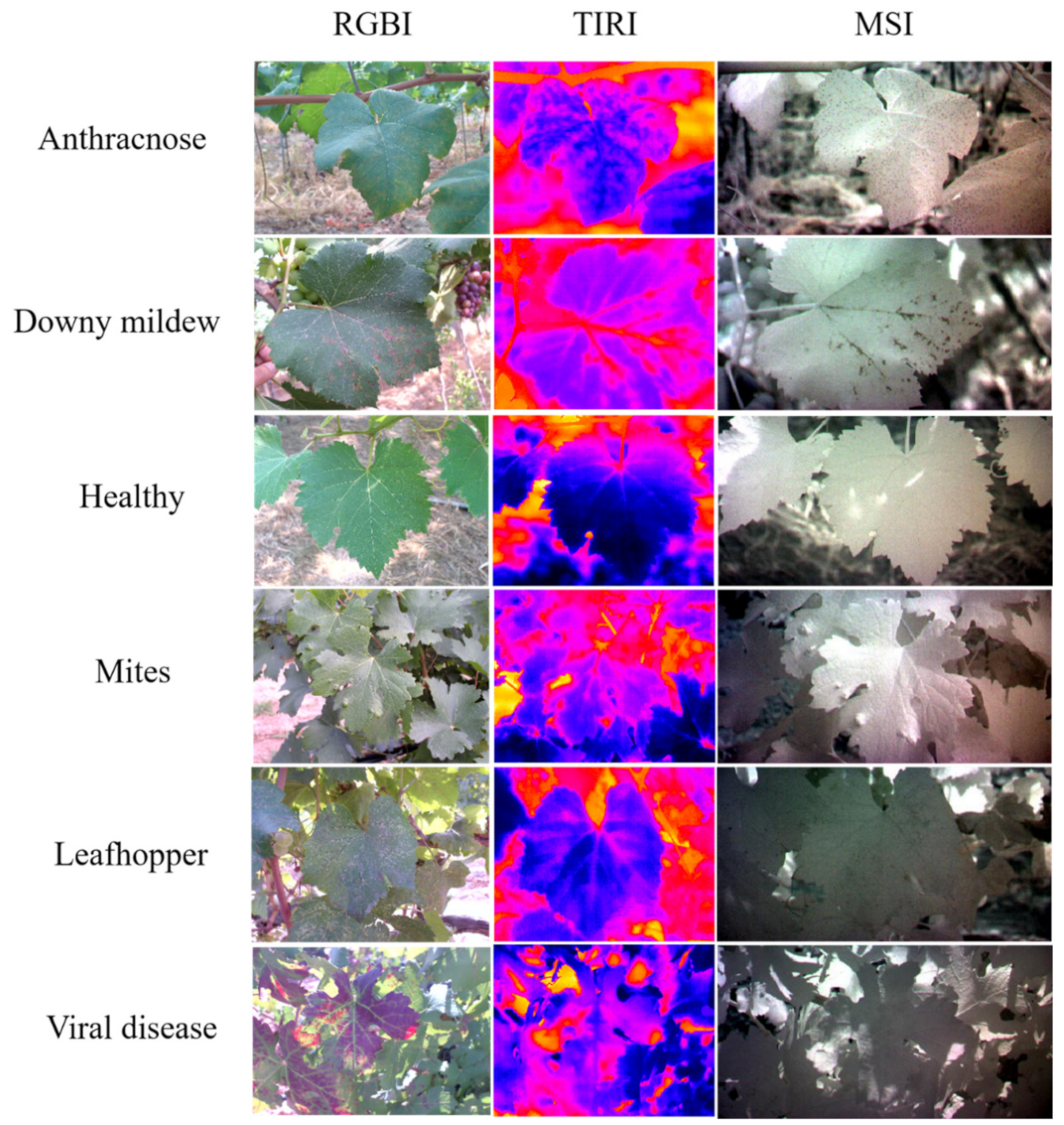
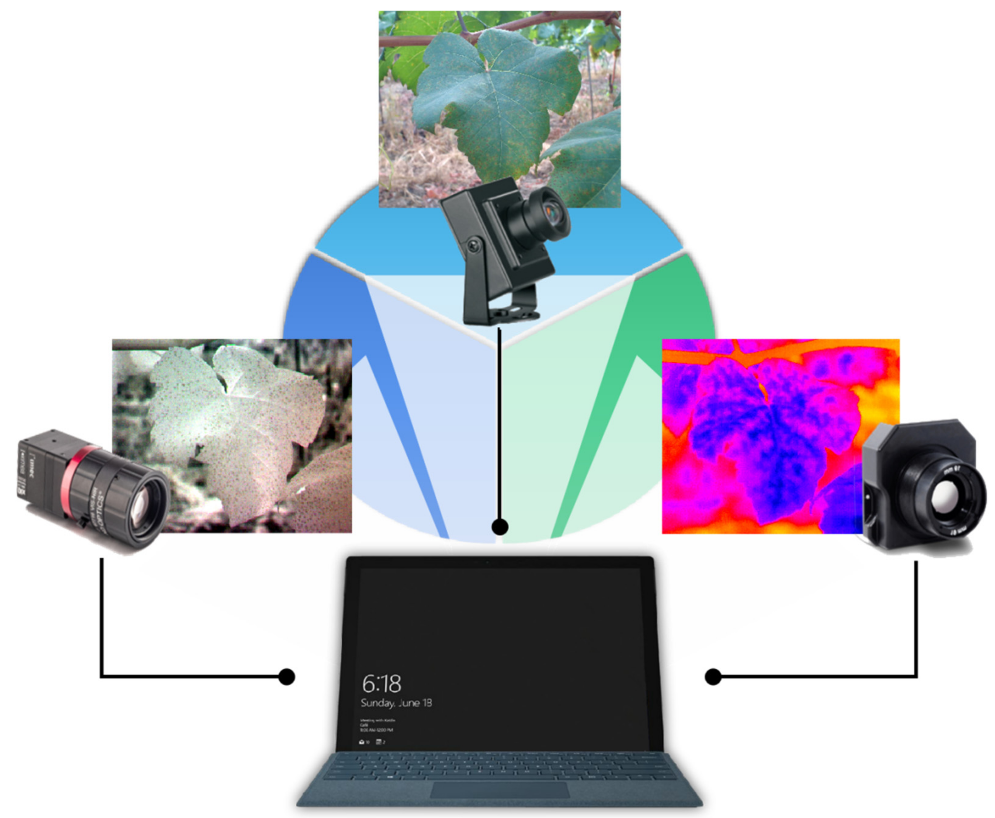
2.1. Data Acquisition

In total, 834 groups of grape foliage images were collected under rainless weather conditions with illumination from 8000 to 46,000 lux. Each group contained three types of images of grape foliage: RGBI (2592 × 1944, 3 channels), MSI (409 × 216, 25 channels), and TIRI (640 × 512, 3 channels), obtained by the RGB camera (LRCP Luoke, USB camera), MS camera with 25 bands (XIMEA, MQ022HG-IM-SM5 × 5 NIR), and TIR camera (FILR, Tau2-640), respectively. The three cameras were combined into a portable device. RGBI, MSI, and TIRI could be acquired by corresponding cameras, which were directly controlled by a portable computer while field sampling (Figure 1). During each collection of images, one grape leaf was selected to be the detection object and located in the middle of the camera view field as much as possible. The total images included six classes: anthracnose, downy mildew, leafhopper (Erythroneura apicalis Nawa), mites (Colomerus (Eriophyes) vitis), viral disease (grapevine leafrool-associated virus, grapevine fanleaf virus etc.), and healthy classes. They were collected from two regions in China: Hangzhou, Zhejiang (HZ), and Yinchuan, Ningxia Hui Autonomous Region (YC). The details of grape foliage image set are illustrated in

Table 1. Details of six classes of grape foliage diseases and pests in the image set. “HZ” refers to Hangzhou, Zhejiang. “YC” refers to Yinchuan, Ningxia Hui Autonomous Region.

Class	Anthracnose	Downy Mildew	Healthy	Mites	Leafhopper	Viral Disease
Collected region	HZ	HZ	HZ	YC	YC	YC
Number of RGBI	168	162	162	120	121	101
Number of MSI	168	162	162	120	121	101
Number of TIRI	168	162	162	120	121	101

. RGBI, TIRI, and MSI of six representative grape foliage diseases and pests are shown in Figure 2. As MSI has 25 channels, for the convenience to display, three channels with wavelengths of 896.2530, 837.1966, and 743.0255 nm were selected to compose RGBI.

As shown in Figure 1, for anthracnose class, small spots are densely distributed on the leaf, with brown in the middle and yellow at the edge; for downy mildew class, the leaf surface is light yellow to reddish-brown, with white frosty mildew on the back; for mites class, the surface of the leaf is blistered; for leafhopper class, the pests would absorb the sap from the leaves, leading to the white spots because of green fading. Therefore, white spots are on the surface of leaf, becoming pieces in severe cases; for virus class, when leaf foliage is infected by viruses, it often shows a variety of symptoms, for example, the leaf becomes curly and purple-red in the infection of grapevine leafrool-associated virus, the leaf changes to fanleaf in the infection of grapevine leafrool-associated virus. The main symptoms of the samples in viral disease class we collected were curly and locally purple-red leaves; for healthy control class, the leaf surface is green without spot.

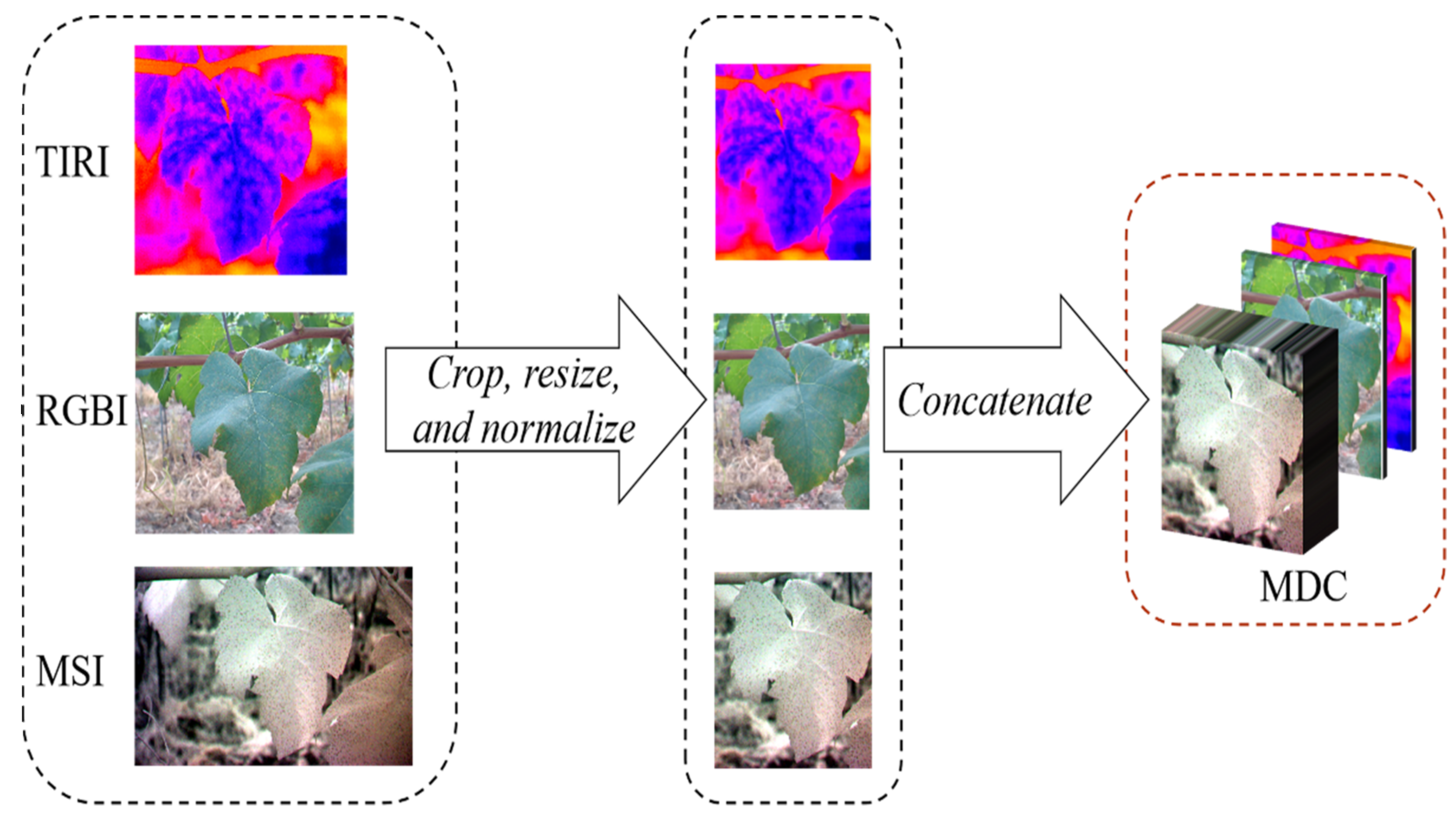
2.2. Data Preprocessing

In order to make the detected grape leaf fill the image as much as possible, the RGBI, MSI, and TIRI were cropped along the center into pixel sizes as follows: 1900 × 1900, 192 × 192, 512 × 512. All images were resized to 192 × 192 considering the different resolutions of the three types of images. Then, the images were normalized to (−1, 1) to accelerate the subsequent network calculations for better detection [34]. Considering to compare the detection performance of MSI, RGBI, and TIRI models for the same sample, the input sequence of samples in MSI, RGBI, and TIRI set needed to be kept the same during the model training. Therefore, according to the sequence of MSI, RGBI, and TIRI, three types of images were concatenated into one new data with 31 channels to form the multi-source data concatenation (MDC) set. Therefore, the RGBI, MSI, and TIRI sets could be obtained according to the corresponding channel ranges from the MDC set with fixed order. The data preprocessing is shown in Figure 3.

Considering the differences in data volume of six classes and the percentage of samples for each class, the total of 834 new data in the MDC set were divided into three parts according to the proportion of total sample size during data division. In total, 20% of the six classes in MDC set were randomly divided as the MDC test set. The remaining data were cross-validated by five-fold and divided into MDC training set and MDC validation set by the ratio of 4:1 in each fold.

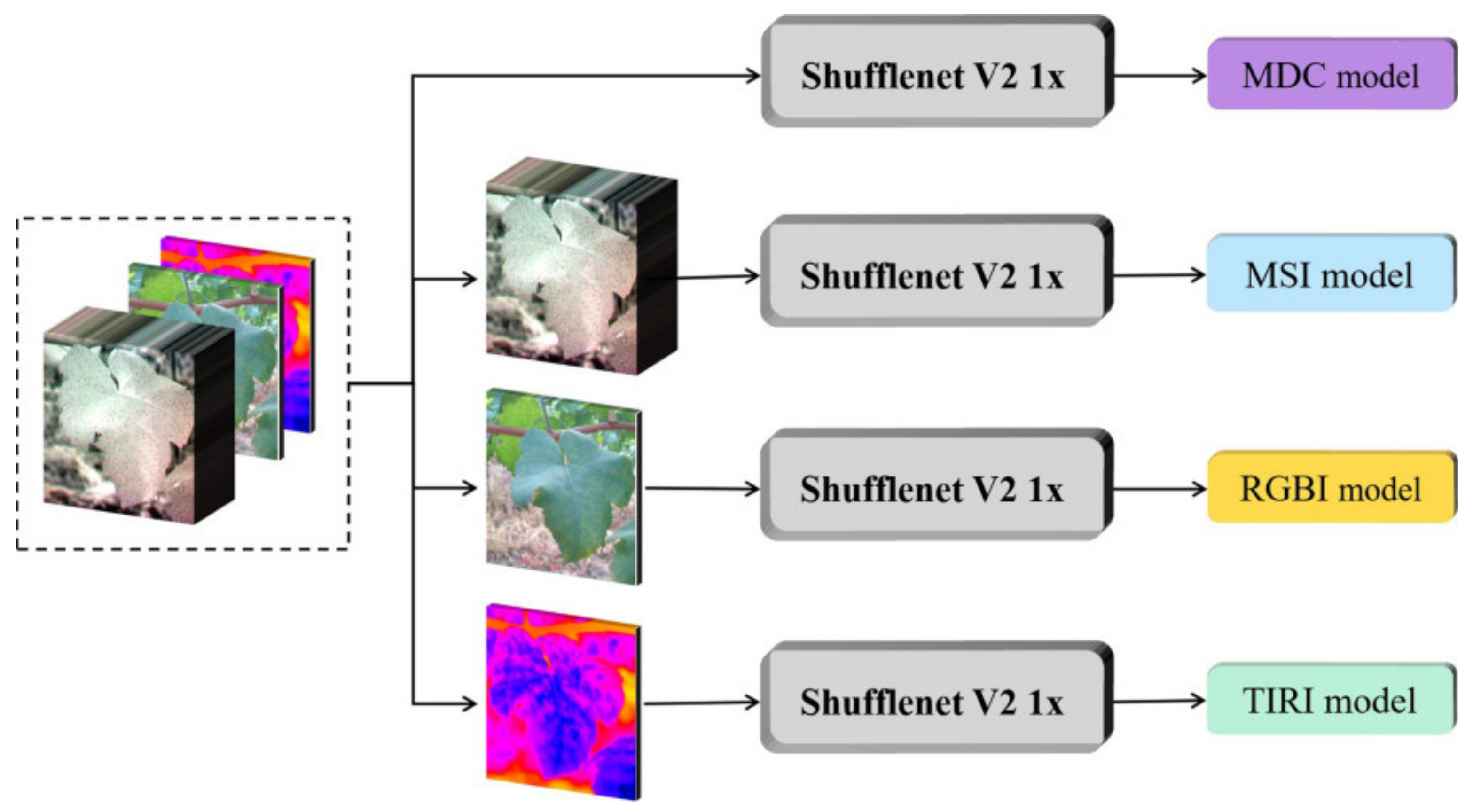
2.3. Detection Model

ShuffleNet V2 was proposed by Ma et al. in 2018 [35]. It is an improvement on ShuffleNet V1, which is an extremely efficient convolutional neural network for mobile devices [13]. ShuffleNet V2 not only introduces “channel shuffle” to enable the information communication between channels, but also is designed based on four practical guidelines for efficient network design.

Firstly, the input of feature channels is split into two branches. One branch remains to reduce network fragmentation and improve the degree of parallelism. The other branch consists of three convolutions with the same input and output channels to make channel width equally and minimize memory access cost (MAC). Then, two 1 × 1 convolutions replace group-wise, which also decreases MAC. After three convolutions, the two branches are concatenated instead of the “Add” operation to keep the number of channels the same. After the same “Channel Shuffle” operation, the next unit begins. Element-wise operations only exist in one branch to reduce the operations like rectified linear unit (ReLU) function and depthwise convolutions. Additionally, “Concat”, “Channel Shuffle”, and “Channel Split”, are merged into a single element-wise operation [35].

In our study, the stride was set to 1, and ShuffleNet V2 1× was selected as the lightweight network for disease and pest detection of grape foliage, while 1× represented different complexities of networks.

2.4. Modeling Setup

All modeling processes were conducted on the same system with details in

Table 2. Software and hardware environments.

Configuration	Value
Central processing unit	Intel Corei7-10750H
Graphics processor unit	NVIDIA Quadro RTX 5000 with Max-Q Design
Operation system	Windows 10
Deep learning framework	PyTorch

. Additionally, the PyTorch library was used to implement the models on the Python platform.

The hyperparameters related to training algorithm in this study included learning rate, training epoch, optimizer, batch size, and so on. The detailed settings were as follows. The initial learning rate and training epoch were set to 0.01 and 80. Learning rate was adjusted flexibly by the ReduceLROnPlateau scheduler, which could dynamically update the learning rate. This scheduler read the training loss of each epoch and if no dropping was seen for 7 consecutive epochs, the learning rate would be reduced by 50%. Additionally, the model parameters of the epoch with the best accuracy on the validation set would be saved during the model training. The Adam optimizer was used to update the learning rate with gradient descent adaptively. It can acquire good accuracy with faster speed, compared with the SGD algorithm [36]. Batch size was set to 64 to accelerate convergence and improve the model performance. Due to the different number of samples in six classes, taking into account of the classes balance, class weights were set for each class while calculating cross-entropy loss function. The class weights of anthracnose, downy mildew, healthy, mites, leafhopper, and viral disease were 4.96, 5.15, 5.15, 6.95, 6.89, and 8.26, respectively. In addition, pretrained parameters provided by PyTorch library were added to the model training process to speed up model fitting. Random seeds were fixed to ensure the reproducibility of the experiments.

In this study, the overall accuracy and F1 score after five-fold cross-validation were selected to evaluate the performance of models. The overall accuracy can be obtained by averaging the accuracy of model detection on the test set in each fold. F1 score is the harmonic average of precision and recall, which reflects the specificity and sensitivity of models. It is a common indicator in classification problems [37]. The total number of network parameters (Total params) and theoretical amount of multiply-adds (MAdds) were used to assess the potential of models for mobile devices. Total params can represent the size of models, and MAdds is the number of multiply-accumulate operations [17].

3. Results

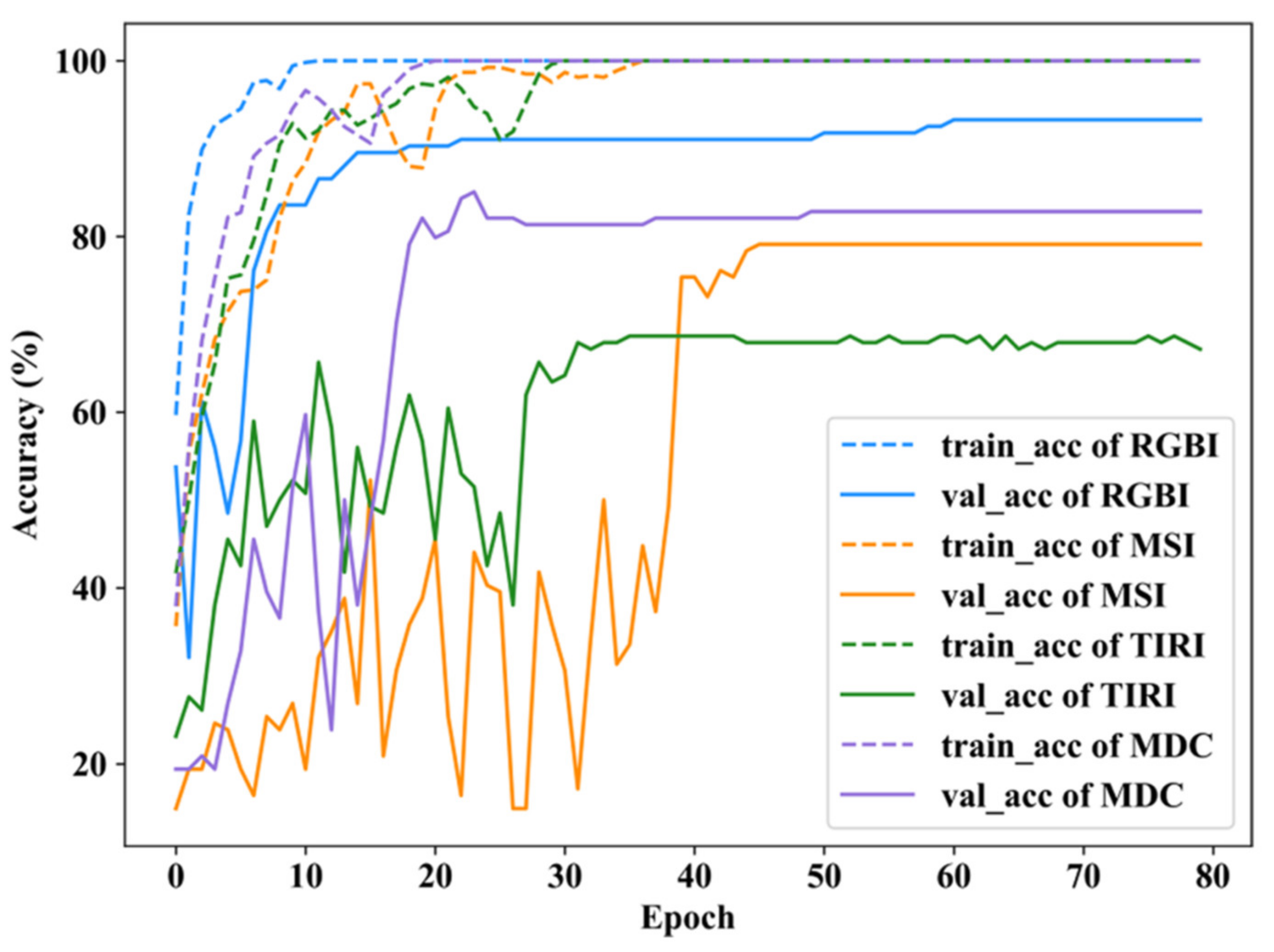
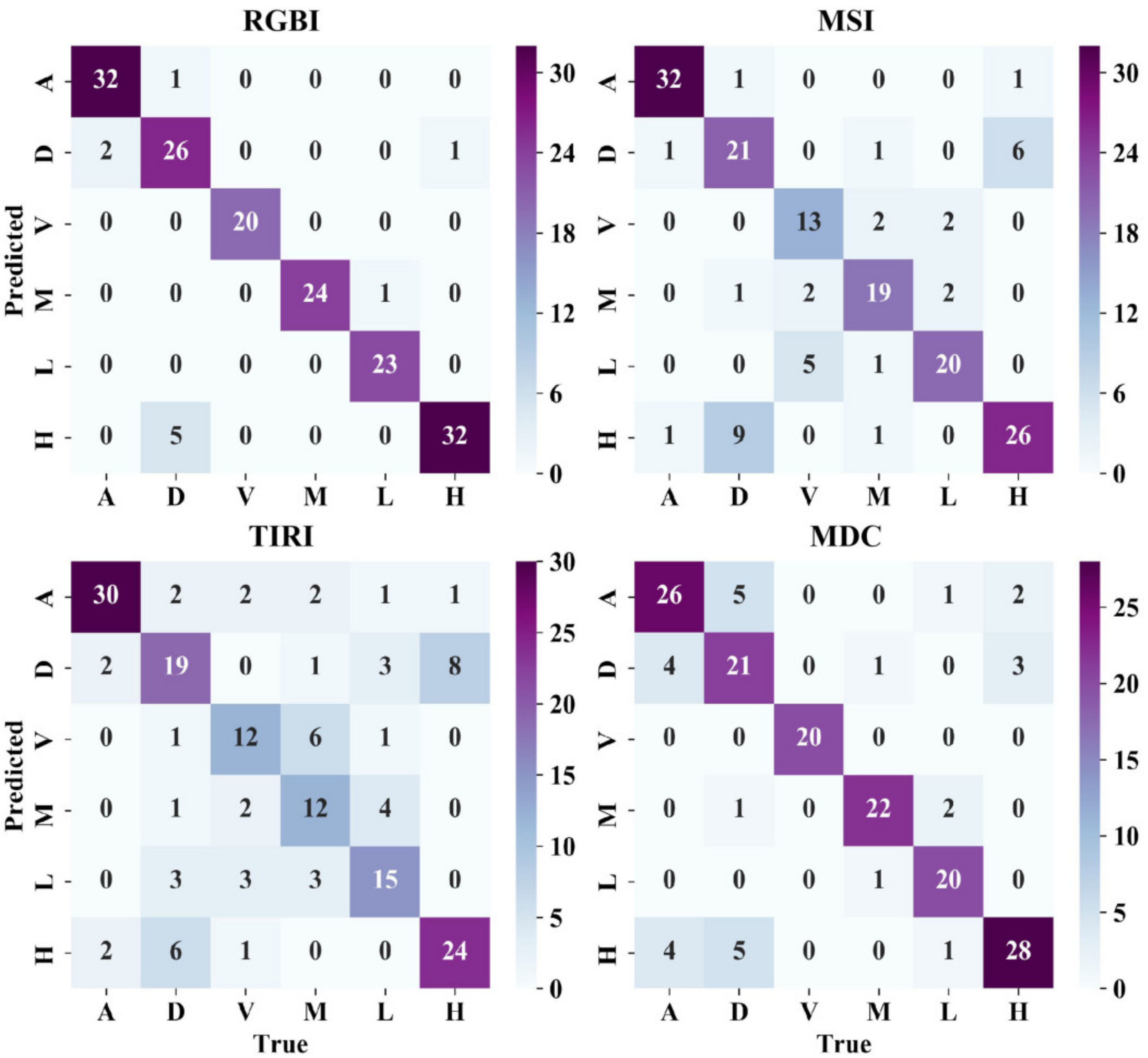
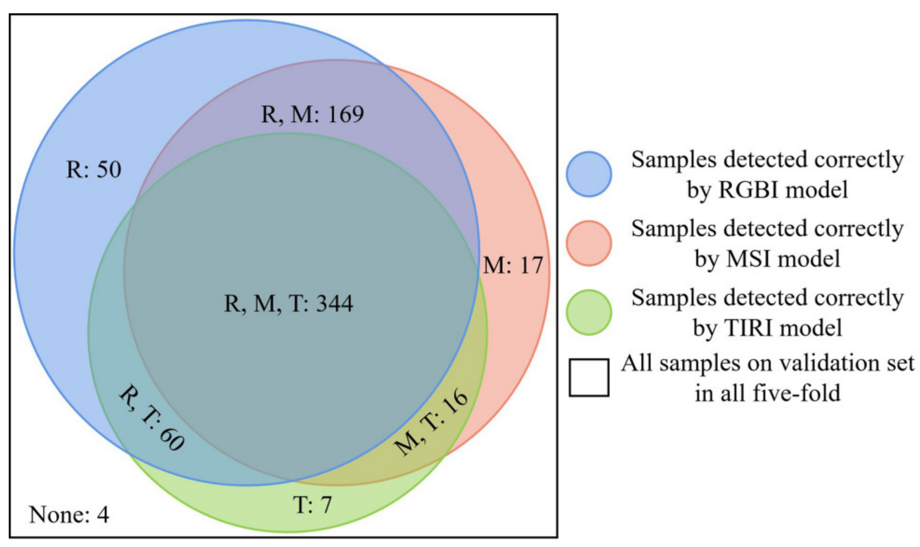
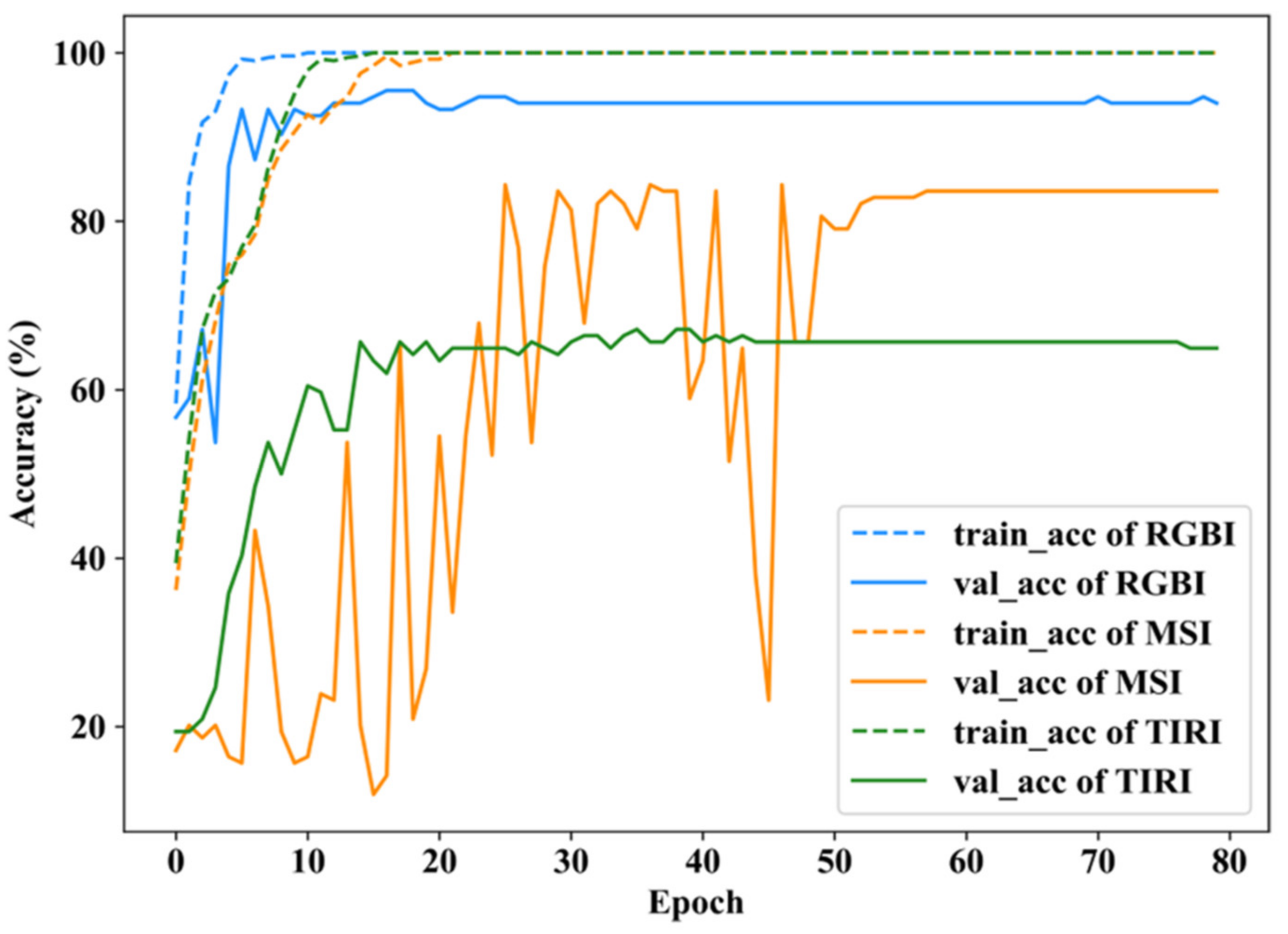
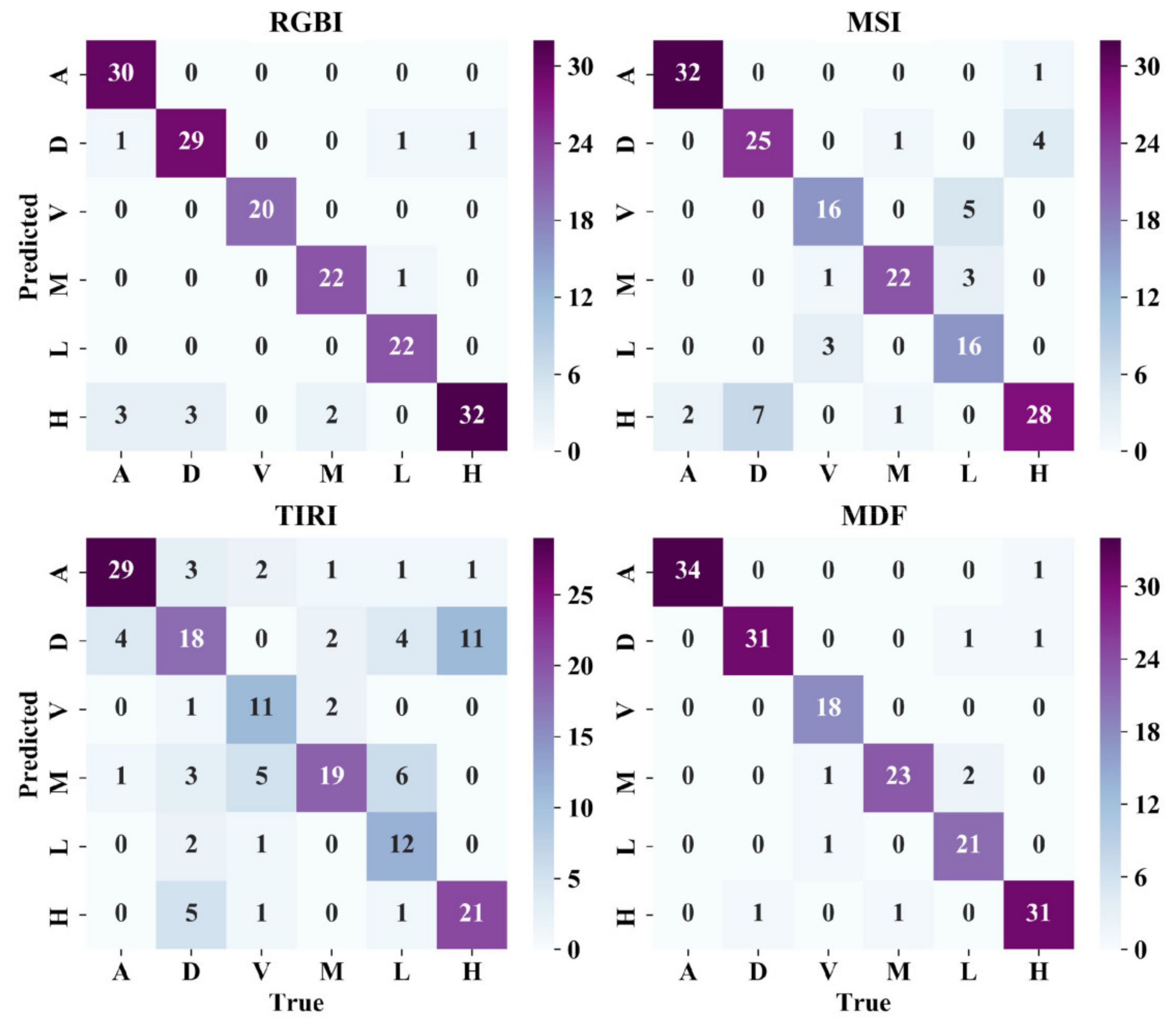
3.1. Results of RGBI, MSI, TIRI, and MDC Models

RGBI, MSI, TIRI, and MDC models of grape foliage detection were obtained based on ShuffleNet V2, as shown in Figure 4. The performances of four models in the first fold are shown in Figure 5. The overall accuracy and F1 score of the four models on the test set were compared (

Table 3. Overall accuracy and F1 score of RGBI, MSI, TIRI, and MDC models.

	F1 Score						Overall Accuracy
	Anthracnose	Downy Mildew	Viral Disease	Mites	Leafhopper	Healthy
RGBI	0.9384	0.8711	1.0000	0.9794	0.9654	0.9121	93.77%
MSI	0.9364	0.7030	0.7307	0.8621	0.7946	0.7424	79.88%
TIRI	0.7731	0.5690	0.6118	0.5964	0.6282	0.6765	64.91%
MDC	0.7879	0.7226	0.9738	0.9098	0.8930	0.7987	83.23%

). In order to demonstrate the detection performances of the four models, the confusion matrices of models on the test set in the first fold are shown in Figure 6.

As shown in Figure 5, all the models were fitted in 80 epochs. As the pretrained ShuffleNet V2 provided by PyTorch library was trained on the dataset consistent with the type of RGBI, the model fitted the fastest on the RGBI set and tended to be convergent in the 23rd epoch. The model trained on the other three sets also converged after fluctuation.

On the test set, as illustrated in Table 3, the RGBI model got the best performance with an overall accuracy of 93.77%. The overall accuracy of MDC model was 83.23%, which had improvements of 3.45% and 18.32%, compared with MSI model and TIRI model, respectively. As for the F1 score, it can be found that RGBI model achieved the best overall detection accuracy in all six classes with 0.9384 for anthracnose class, 0.8711 for downy mildew class, 1.0000 for viral disease, 0.9794 for mites class, 0.9654 for leafhopper class, and 0.9121 for healthy class. While, MDC model was slightly better than MSI model except for anthracnose class.

TIRI model had the worst performance among the three models. The poor performance of the model can be explained by the influence of the complicated environment of vineyard on TIR imaging. The thermal image can reflect the heat distribution field [29] on the surface of the grape foliage, however, the temperature of grape foliage is greatly affected by the environment. It could also be found that the temperature of grape foliage exposed to direct sunlight was significantly higher than that of grape foliage without direct sunlight when collecting TIRI, and the ambient temperature of the former was also higher, which had great interference to TIR imaging.

In the confusion matrices of the first fold (Figure 6), the performance of the RGBI model was superior to the MDC model for all six classes. The detection performance of the MDC model in each class was slightly better than MSI model in general, but the result of anthracnose class was inferior to the MSI model, which was consistent with the F1 score values of MDC model and MSI model (Table 3).

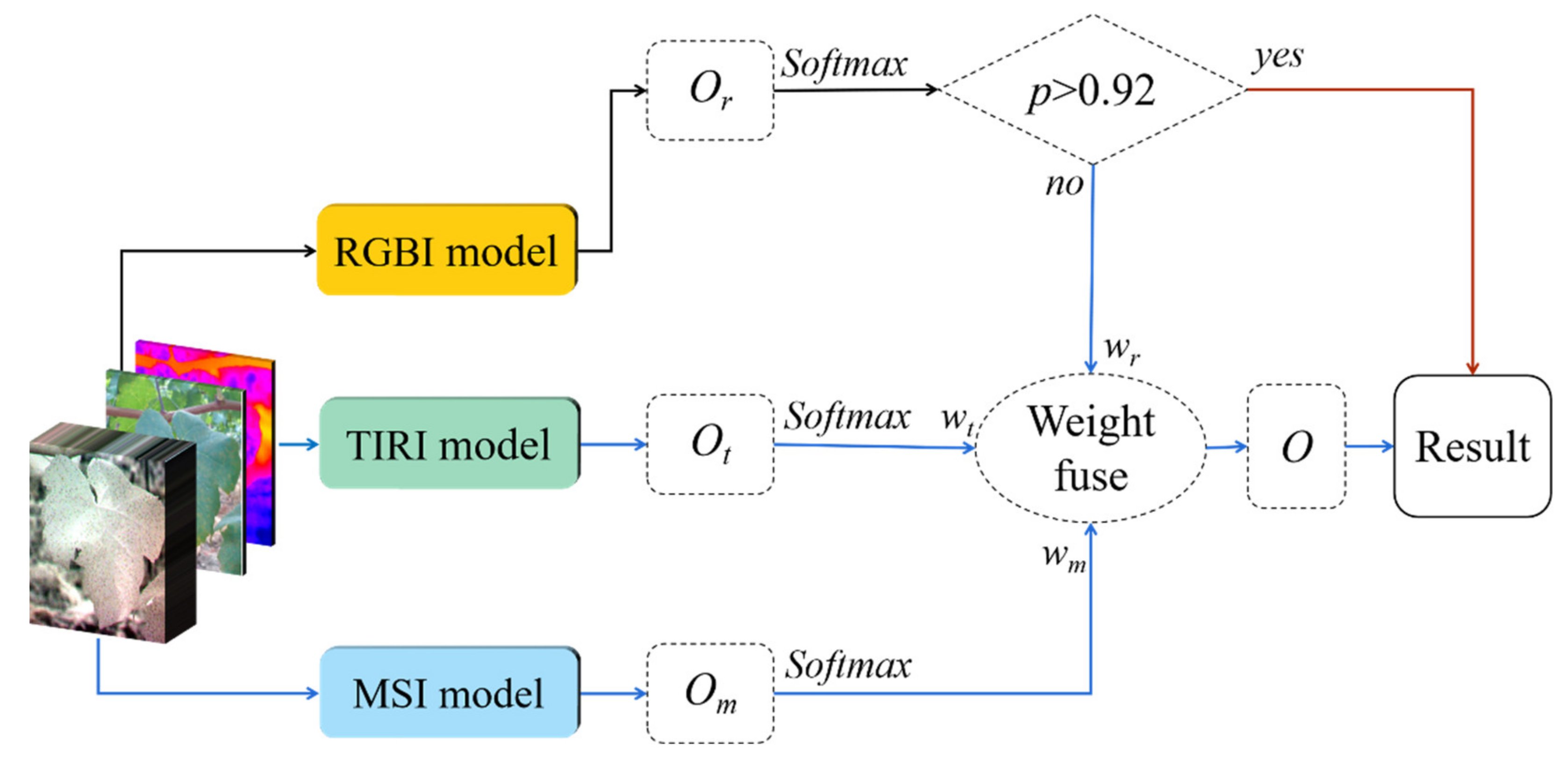
3.2. MDF Decision-Making Method

3.2.1. Outputs of RGBI, MSI, and TIRI Models

In this section, the outputs’ correctness of RGB, MSI, and TIRI models are compared. Based on the experiments in Section 3.1, the numbers of samples correctly detected by RGBI, MSI, and TIRI models on the validation set in all five-fold were analyzed (Figure 7). As shown in Figure 7, 51.57% of the total samples could be correctly detected by all three models, and 11.09% of the total samples got correct detection results uniquely by one of the three models. It cannot be ignored that 40 of 44 samples incorrectly detected by RGBI model could be correctly detected by MSI model or TIRI model. This confirmed that MSI model and TIRI model could be considered to assist the decision-making of RGBI model, so that the incorrect detections made by RGBI model could be rectified.

The softmax function is a normalized exponential function, which is used to present the results of multiple categories as probabilities [38]. Therefore, the softmax function after the three models’ fully connected layer was added for intuitive observation of the outputs that led to the model decision directly. The class index corresponding to the maximum predicted score, which is also the maximum probability (p) of the output through the softmax layer is the model’s detection result. Additionally, p can be regarded as the detection credibility of the model, it is also the confidence of the model’s output. The p’s distribution proportion of samples detected by RGBI model on the validation set in all five-fold were compared (

Table 4. p’s distribution of samples detected by RGBI model. “Right” represents correctly detected samples, “Wrong” represents incorrectly detected samples.

	Distribution Proportion
	(0, 0.5]	(0.5, 0.55]	(0.55, 0.6]	(0.6, 0.65]	(0.65, 0.7]	(0.7, 0.75]	(0.75, 0.8]	(0.8, 0.85]	(0.85, 0.9]	(0.9, 0.95]	(0.95, 1]
Right	1.61%	0.32%	0.00%	0.48%	0.32%	0.16%	1.12%	1.61%	1.61%	3.53%	89.25%
Wrong	11.36%	0.00%	2.27%	2.27%	2.27%	4.55%	11.36%	9.09%	2.27%	11.36%	43.18%

). As illustrated in Table 4, the distribution of p was very dense in the range between 0.9 and 1. p of 92.78% correctly detected samples were over 0.9, and p of more than 50% incorrectly detected samples were more than 0.9. Meanwhile, 43.18% incorrectly detected samples had p values over 0.95, which led to the mixture of these samples and correctly detected samples. They were difficult to detect. In other words, for the samples detected incorrectly, the model’s confidence for results was too high, indicating that the RGBI model had the problem of overconfidence. Guo et al. [39] also proposed that the accuracy of model did not match its prediction confidence, so the model needed to be calibrated.

3.2.2. Outputs of RGBI, MSI, and TIRI Models with Label Smoothing

Label smoothing was adopted for model calibration in this study. Label smoothing is a widely used “trick” to prevent the model from becoming over-confident and improve model performance. It changes the training goal of the model from “1” to “1-label smoothing adjustment”, so the model can be less confident about its output [40]. With label smoothing, models also converged well in 80 epochs (Figure 8). To verify that label smoothing inhibited model overconfidence, the detection outputs of each fold by RGBI model with label smoothing on the validation set were taken out, and the corresponding p of samples after softmax layer were obtained. Meanwhile, the p’s distribution proportion of samples detected by RGBI model with label smoothing on the validation set in all five-fold is shown in

Table 5. p’s distribution of samples detected by RGBI model. “Right” represents correctly detected samples, “Wrong” represents incorrectly detected samples. “LS” represents the sample detected by RGBI model with label smoothing, and “Change” refers to the proportion change of p in the distribution interval after label smoothing.

	Distribution Proportion
	(0, 0.5]	(0.5, 0.55]	(0.55, 0.6]	(0.6, 0.65]	(0.65, 0.7]	(0.7, 0.75]	(0.75, 0.8]	(0.8, 0.85]	(0.85, 0.9]	(0.9, 0.95]	(0.95, 1]
Right-LS	3.44%	1.56%	1.09%	2.34%	3.13%	3.75%	4.69%	8.91%	23.13%	36.25%	11.72%
Change	+1.83%	+1.24%	+1.09%	+1.86%	+2.80%	+3.59%	+3.56%	+7.30%	+21.52%	+32.72%	−77.53%
Wrong-LS	18.52%	3.70%	11.11%	3.70%	14.81%	7.41%	3.70%	7.41%	7.41%	22.22%	0.00%
Change	+7.15%	+3.70%	+8.84%	+1.43%	+12.54%	+2.86%	−7.66%	−1.68%	+5.13%	+10.86%	−43.18%

.

As shown in Table 5, it was very obvious that p of most samples were distributed to smaller intervals, compared with p’s distribution of samples detected by RGBI model without label smoothing. This indicated that label smoothing worked well. For correctly detected samples, most p were distributed between 0.85 and 0.95, and the proportion of p that was over 0.9 was reduced by 44.81%. For the incorrectly detected samples, the distribution of p was lack of concentration, which was mainly around 0.55, 0.65, and 0.9. There was a significant increase (36.53%) of p’s proportion between 0 and 0.75, compared with the distribution without label smoothing. Additionally, p of incorrectly detected samples were all less than 0.95, which meant that one sample could be correctly detected by RGBI model if the sample’s p was over the maximum p of all incorrectly detected samples.

3.2.3. MDF Model

The average value ($\overline{p}=0.92$) of the maximum p of incorrectly detected samples on the validation set in all five-fold was set to be the threshold value. This threshold was the critical value to decide whether we accepted the RGBI model’s detection result. The detection result of RGBI model can be believed if p > 0.92. As for p ≤ 0.92, the overall accuracy of RGBI model, MSI model, and TIRI model would be introduced as the weight w. The outputs of the same sample after softmax layer of RGBI (O_r), MSI (O_m), and TIRI models (O_t) would be respectively multiplied by the corresponding weight w_r, w_m, and w_t. Then, the outputs after introducing weights would be added up, and divided by the sum of the weights. Additionally, the final detection output O would be obtained, as shown in Equation (1). The simple sum of the outputs of models was not directly used, because RGBI, MSI, and TIRI models had different overall accuracy, and the values could be introduced as the overall reliability of the relevant models to further punish the prediction confidence of the models.

Meanwhile, as illustrated in Table 5, it could be noticed that label smoothing also inhibited the confidence of correct detection results detected by RGBI model. With label smoothing, for correctly detected samples, the proportion of p that was more than 0.95 was significantly reduced by 77.53% and only 47.97% p were over 0.9. It was an unexpected result that the outputs of samples correctly detected by RGBI model were changed and the samples were detected again because p ≤ 0.92. To overcome the problem, during the MDF decision-making process, O_m and O_t would be punished because of the lower detection accuracy of the MSI model and TIRI model compared with RGBI model. Additionally, O_r was more trusted to decrease the probability of misclassification of samples detected correctly by RGBI model. The data processing in MDF model based on MDF decision-making method is shown in Figure 9.

$$O=\left\{\begin{array}{ccc}\frac{O_r\cdot w_r+O_m\cdot w_m+O_t\cdot w_t}{w_r+w_m+w_t}& ,& p\le 0.92\\ & & \\ O_r& ,& p>0.92\end{array}\right.$$

(1)

3.2.4. Result of MDF Model

Based on the MDF decision-making method, the detection performance of MDF model was compared with RGBI, MSI, and TIRI models by overall accuracy and F1 score in all five-fold (

Table 6. Overall accuracy and F1 score of RGBI, MSI, TIRI, and MDF models.

	F1 Score						Overall Accuracy
	Anthracnose	Downy Mildew	Viral Disease	Mites	Leafhopper	Healthy
RGBI	0.9464	0.8633	1.0000	0.9832	0.9616	0.8930	93.41%
MSI	0.9414	0.7520	0.7684	0.8619	0.8207	0.7784	82.40%
TIRI	0.8399	0.5610	0.7007	0.7103	0.6163	0.6709	68.26%
MDF	0.9826	0.9233	0.9846	0.9840	0.9783	0.9283	96.05%

). Additionally, the confusion matrices of four models on the test set in the first fold are shown in Figure 10.

In terms of overall accuracy, the proposed method improved the value of RGBI model by 2.64%, which meant that the MDF model had corrected 40% of the wrong detection results of RGBI model. According to the F1 score, the RGBI model had a relatively poor performance in anthracnose, downy mildew, and healthy classes, which was also reflected in the confusion matrices (Figure 10). Compared with RGBI model, MDF model improved the F1 scores of anthracnose, downy mildew, and healthy classes, and had an increase of 3.83%, 6.95%, and 3.95%, respectively.

Moreover, the performances of MDF model in six classes were also better than RGBI model, except for 0.0154 lower in viral disease class. The confusion matrix in the fourth fold explained the reduction (Figure 11). F1 score is a comprehensive index obtained by recall and precision. In the fourth fold, MDF model was correct for all the samples in viral disease class, so the recall value was 100%. However, RGBI model was not confident enough for the samples in leafhopper class. p of this incorrectly detected sample was 0.8845, which led to the re-detection of the sample through MDF decision-making method. MSI model and TIRI model detected the sample incorrectly to be viral disease class due to their consistent propensity for viral disease class about this sample. Therefore, the precision value of viral disease class was reduced to 95.24%. Finally, there was a reduction of F1 score in viral disease class.

3.3. Lightweight of MDF Model

Considering that if p ≤ 0.92, the MDF decision-making method used in MDF model was equivalent to detect by RGBI, MSI, and TIRI models together. Therefore, the total params and MAdds of MDF model were the accumulation of the corresponding values of RGBI, MSI, and TIRI models. As shown in

Table 7. Total number of network parameters (Total params) and theoretical amount of multiply-adds (MAdds) of models.

Model	Total Params	MAdds
MobileNet V2 and MobileNeXt	1.7~6.9 M	0.059~0.690 G
RGBI model	1.260 M	0.106 G
MSI model	1.265 M	0.150 G
TIRI model	1.260 M	0.106 G
MDF model	3.785 M	0.362 G

, the results were 3.785 M and 0.362 G. They were acceptable, compared with the values of MobileNet V2 and MobileNeXt, whose classification performance and latency had been tested on Google Pixel 4XL and performed well [41]. This meant that the MDF model had potential for mobile devices.

4. Discussion

The main features between healthy and unhealthy grape foliage in our dataset used for detection lay on the differences of leaf texture information, color change, and leaf shape changing, etc. These features were easy to be recognized and captured clearly in the RGBI, which could be the reason for the best performance of the RGBI model. As for the MDC model and MSI model, due to a large number of channels, the feature dimension was too large and the information of features was redundant [42]. Therefore, even though the data had been normalized, it was still not conducive for MDC model and MSI model to learn features for detection. There is also abundant room for further progress in reducing feature redundancy after the concatenation of RGBI, MSI, and TIRI for detection. As for the MDC model, the overall accuracy and F1 score of MDC model had improved compared with MSI model because the MDC set contained RGBI. Although the TIRI model had the worst performance, the detection significance of TIRI cannot be negated. This is because when grape foliage is infected with diseases, the changes on the foliage may influence the heat transfer in the infected part of the surface to a certain extent. This can lead to local temperature differences of the leaf surface, which are helpful for plant health status detection [43].

Based on the characteristics of RGBI, MSI, and TIRI models, the MDF decision-making method was proposed fully considering the diversity and specificity of RGBI, MSI, and TIRI. The detection advantages of RGBI model remained and then the model was re-examined based on its confidence with label smoothing. When the confidence of detection results did not meet the threshold we set, attention would be paid to MSI and TIRI of the samples being detected. Then, different weights were given to the outputs of MSI model and TIRI model, and the detection results given by the RGBI model were finally modified. Although we punished the outputs by weights, few correctly detected samples would also be screened out and entered the fusion decision-making stage due to the model’s confidence problem, because p of the samples were less than or equal to 0.92. This might lead to misclassification of these samples. Additionally, the small total params and MAdds based on ShuffleNet V2 indicated that the MDF model had great potential in the application of mobile devices.

Generally, with the lightweight network and multi-source data collected in the field, we provided an effective method for MDF decision-making and proposed an improved model with higher precision and good practical application potential, which could be a solution for the disease and pest detection of grape foliage in complicated environments. Possible improvements of this study can be focused on: (1) a more comprehensive selection mechanism, which can only screen out the misclassified samples to get into the MDF decision-making stage for the improvement of the MDF model’s detection accuracy; (2) introduction of more grape foliage classes and other lightweight networks, which may enhance the generalization and performance of the model.

5. Conclusions

In this study, based on the ShuffleNet V2 network, the performance and overall accuracy of the detection results of RGBI (93.77%), MSI (79.88%), TIRI (64.91%), and MDC models (83.23%) were compared. Due to the detection characteristics of the four models, we provided an MDF decision-making method and obtained an MDF model for the disease and pest detection of grape foliage. The method was used to correct the detection results of RGBI model, which had the best performance among the four models. The overall accuracy of MDF model was 96.05%, and 40% of the samples incorrectly detected by RGBI model were rectified. MDF model had an overall accuracy improvement of 2.64%, 13.65%, and 27.79%, respectively, compared with RGBI, MSI, and TIRI models. Meanwhile, for the lightweight network’s introduction, the total params and the MAdds of MDF model were only 3.785 M and 0.362 G. Hence, it could be portable and easy to apply, which would provide a solution and a reference for multi-source data fusion and the application of deep learning detection models of grape foliage diseases and pests in the field.

References

1. Jaisakthi, S.M.; Mirunalini, P.; Thenmozhi, D.; Vatsala. Grape Leaf Disease Identification Using Machine Learning Techniques. In Proceedings of the 2019 International Conference on Computational Intelligence in Data Science (ICCIDS), Chennai, India, 21–23 February 2019; pp. 1–6. [Google Scholar]
2. Pertot, I.; Caffi, T.; Rossi, V.; Mugnai, L.; Hoffmann, C.; Grando, M.S.; Gary, C.; Lafond, D.; Duso, C.; Thiery, D.; et al. A Critical Review of Plant Protection Tools for Reducing Pesticide Use on Grapevine and New Perspectives for the Implementation of IPM in Viticulture. Crop Prot. 2017, 97, 70–84. [Google Scholar] [CrossRef]
3. Nalam, V.; Louis, J.; Shah, J. Plant Defense against Aphids, the Pest Extraordinaire. Plant Sci. 2019, 279, 96–107. [Google Scholar] [CrossRef]
4. Wu, A.; Zhu, J.; He, Y. Computer Vision Method Applied for Detecting Diseases in Grape Leaf System. In Cognitive Internet of Things: Frameworks, Tools and Applications; Lu, H., Ed.; Studies in Computational Intelligence; Springer International Publishing: Cham, Switzerland, 2020; pp. 367–376. [Google Scholar]
5. Meunkaewjinda, A.; Kumsawat, P.; Attakitmongcol, K.; Srikaew, A. Grape Leaf Disease Detection from Color Imagery Using Hybrid Intelligent System. In Proceedings of the 2008 5th International Conference on Electrical Engineering/Electronics, Computer, Telecommunications and Information Technology, Krabi, Thailand, 14–17 May 2008; pp. 513–516. [Google Scholar]
6. Sannakki, S.S.; Rajpurohit, V.S.; Nargund, V.B.; Kulkarni, P. Diagnosis and Classification of Grape Leaf Diseases Using Neural Networks. In Proceedings of the 2013 Fourth International Conference on Computing, Communications and Networking Technologies (ICCCNT), Tiruchengode, India, 4–6 July 2013; pp. 1–5. [Google Scholar]
7. Khirade, S.D.; Patil, A.B. Plant Disease Detection Using Image Processing. In Proceedings of the 2015 International Conference on Computing Communication Control and Automation, Pune, India, 26–27 February 2015; pp. 768–771. [Google Scholar]
8. Padol, P.B.; Yadav, A.A. SVM Classifier Based Grape Leaf Disease Detection. In Proceedings of the 2016 Conference on Advances in Signal Processing (CASP), Pune, India, 9–11 June 2016; pp. 175–179. [Google Scholar]
9. Padol, P.B.; Sawant, S.D. Fusion Classification Technique Used to Detect Downy and Powdery Mildew Grape Leaf Diseases. In Proceedings of the 2016 International Conference on Global Trends in Signal Processing, Information Computing and Communication (ICGTSPICC), Jalgaon, India, 22–24 December 2016; pp. 298–301. [Google Scholar]
10. LeCun, Y.; Bengio, Y.; Hinton, G. Deep Learning. Nature 2015, 521, 436–444. [Google Scholar] [CrossRef]
11. Liu, B.; Ding, Z.; Tian, L.; He, D.; Li, S.; Wang, H. Grape Leaf Disease Identification Using Improved Deep Convolutional Neural Networks. Front. Plant Sci. 2020, 11, 1082. [Google Scholar] [CrossRef]
12. Ji, M.; Zhang, L.; Wu, Q. Automatic Grape Leaf Diseases Identification Via UnitedModel Based on Multiple Convolutional Neural Networks. Inf. Process. Agric. 2020, 7, 418–426. [Google Scholar] [CrossRef]
13. Zhang, X.; Zhou, X.; Lin, M.; Sun, J. Shufflenet: An Extremely Efficient Convolutional Neural Network for Mobile Devices. In Proceedings of the IEEE/CVF Conference on Computer Vision and Pattern Recognition, Salt Lake City, UT, USA, 18–23 June 2018; pp. 6848–6856. [Google Scholar]
14. Iandola, F.N.; Han, S.; Moskewicz, M.W.; Ashraf, K.; Dally, W.J.; Keutzer, K. SqueezeNet: AlexNet-Level Accuracy with 50x Fewer Parameters and <0.5 mb Model Size. arXiv 2016, arXiv:1602.07360. [Google Scholar]
15. Howard, A.G.; Zhu, M.; Chen, B.; Kalenichenko, D.; Wang, W.; Weyand, T.; Andreetto, M.; Adam, H. Mobilenets: Efficient Convolutional Neural Networks for Mobile Vision Applications. arXiv 2017, arXiv:1704.04861. [Google Scholar]
16. Sandler, M.; Howard, A.; Zhu, M.; Zhmoginov, A.; Chen, L.-C. Mobilenetv2: Inverted Residuals and Linear Bottlenecks. In Proceedings of the IEEE/CVF Conference on Computer Vision and Pattern Recognition, Salt Lake City, UT, USA, 18–23 June 2018; pp. 4510–4520. [Google Scholar]
17. Howard, A.; Sandler, M.; Chu, G.; Chen, L.-C.; Chen, B.; Tan, M.; Wang, W.; Zhu, Y.; Pang, R.; Vasudevan, V. Searching for Mobilenetv3. In Proceedings of the IEEE/CVF International Conference on Computer Vision, Seoul, Korea, 27 October–2 November 2019; pp. 1314–1324. [Google Scholar]
18. Tan, M.; Le, Q. Efficientnet: Rethinking Model Scaling for Convolutional Neural Networks. In Proceedings of the 36th International Conference on Machine Learning, Long Beach, CA, USA, 9–15 June 2019; pp. 6105–6114. [Google Scholar]
19. Tang, Z.; Yang, J.; Li, Z.; Qi, F. Grape Disease Image Classification Based on Lightweight Convolution Neural Networks and Channelwise Attention. Comput. Electron. Agric. 2020, 178, 105735. [Google Scholar] [CrossRef]
20. Chaerle, L.; Van Caeneghem, W.; Messens, E.; Lambers, H.; Van Montagu, M.; Van Der Straeten, D. Presymptomatic Visualization of Plant-Virus Interactions by Thermography. Nat. Biotechnol. 1999, 17, 813–816. [Google Scholar] [CrossRef] [PubMed]
21. Farber, C.; Mahnke, M.; Sanchez, L.; Kurouski, D. Advanced Spectroscopic Techniques for Plant Disease Diagnostics. A Review. TrAC Trends Anal. Chem. 2019, 118, 43–49. [Google Scholar] [CrossRef]
22. Qin, Z.; Zhang, M. Detection of Rice Sheath Blight for In-Season Disease Management Using Multispectral Remote Sensing. Int. J. Appl. Earth Obs. Geoinf. 2005, 7, 115–128. [Google Scholar] [CrossRef]
23. Mahlein, A.-K.; Steiner, U.; Dehne, H.-W.; Oerke, E.-C. Spectral Signatures of Sugar Beet Leaves for the Detection and Differentiation of Diseases. Precis. Agric. 2010, 11, 413–431. [Google Scholar] [CrossRef]
24. Kerkech, M.; Hafiane, A.; Canals, R. VddNet: Vine Disease Detection Network Based on Multispectral Images and Depth Map. Remote Sens. 2020, 12, 3305. [Google Scholar] [CrossRef]
25. Fahrentrapp, J.; Ria, F.; Geilhausen, M.; Panassiti, B. Detection of Gray Mold Leaf Infections Prior to Visual Symptom Appearance Using a Five-Band Multispectral Sensor. Front. Plant Sci. 2019, 10, 628. [Google Scholar] [CrossRef] [Green Version]
26. Veys, C.; Chatziavgerinos, F.; AlSuwaidi, A.; Hibbert, J.; Hansen, M.; Bernotas, G.; Smith, M.; Yin, H.; Rolfe, S.; Grieve, B. Multispectral Imaging for Presymptomatic Analysis of Light Leaf Spot in Oilseed Rape. Plant Methods 2019, 15, 4. [Google Scholar] [CrossRef]
27. Li, Y.; Wu, F.-X.; Ngom, A. A Review on Machine Learning Principles for Multi-View Biological Data Integration. Brief. Bioinform. 2018, 19, 325–340. [Google Scholar] [CrossRef] [PubMed]
28. Ouhami, M.; Hafiane, A.; Es-Saady, Y.; El Hajji, M.; Canals, R. Computer Vision, IoT and Data Fusion for Crop Disease Detection Using Machine Learning: A Survey and Ongoing Research. Remote Sens. 2021, 13, 2486. [Google Scholar] [CrossRef]
29. Bulanon, D.M.; Burks, T.F.; Alchanatis, V. Image Fusion of Visible and Thermal Images for Fruit Detection. Biosyst. Eng. 2009, 103, 12–22. [Google Scholar] [CrossRef]
30. Mahlein, A.-K.; Alisaac, E.; Al Masri, A.; Behmann, J.; Dehne, H.-W.; Oerke, E.-C. Comparison and Combination of Thermal, Fluorescence, and Hyperspectral Imaging for Monitoring Fusarium Head Blight of Wheat on Spikelet Scale. Sensors 2019, 19, 2281. [Google Scholar] [CrossRef] [Green Version]
31. Feng, L.; Wu, B.; Zhu, S.; Wang, J.; Su, Z.; Liu, F.; He, Y.; Zhang, C. Investigation on Data Fusion of Multisource Spectral Data for Rice Leaf Diseases Identification Using Machine Learning Methods. Front. Plant Sci. 2020, 11, 577063. [Google Scholar] [CrossRef]
32. Prince, G.; Clarkson, J.P.; Rajpoot, N.M. Automatic Detection of Diseased Tomato Plants Using Thermal and Stereo Visible Light Images. PLoS ONE 2015, 10, e0123262. [Google Scholar]
33. Maimaitijiang, M.; Ghulam, A.; Sidike, P.; Hartling, S.; Maimaitiyiming, M.; Peterson, K.; Shavers, E.; Fishman, J.; Peterson, J.; Kadam, S.; et al. Unmanned Aerial System (UAS)-Based Phenotyping of Soybean Using Multi-Sensor Data Fusion and Extreme Learning Machine. ISPRS-J. Photogramm. Remote Sens. 2017, 134, 43–58. [Google Scholar] [CrossRef]
34. Patro, S.; Sahu, K.K. Normalization: A Preprocessing Stage. arXiv 2015, arXiv:1503.06462. [Google Scholar] [CrossRef]
35. Ma, N.; Zhang, X.; Zheng, H.-T.; Sun, J. Shufflenet v2: Practical Guidelines for Efficient CNN Architecture Design. In Proceedings of the European Conference on Computer Vision (ECCV), Munich, Germany, 8–14 September 2018; pp. 116–131. [Google Scholar]
36. Kingma, D.P.; Ba, J. Adam: A Method for Stochastic Optimization. arXiv 2014, arXiv:1412.6980. [Google Scholar]
37. Xu, J.; Yang, J.; Xiong, X.; Li, H.; Huang, J.; Ting, K.C.; Ying, Y.; Lin, T. Towards Interpreting Multi-Temporal Deep Learning Models in Crop Mapping. Remote Sens. Environ. 2021, 264, 112599. [Google Scholar] [CrossRef]
38. Liu, W.; Wen, Y.; Yu, Z.; Yang, M. Large-Margin Softmax Loss for Convolutional Neural Networks. In Proceedings of the 33rd International Conference on Machine Learning, New York, NY, USA, 19–24 June 2016; pp. 507–516. [Google Scholar]
39. Guo, C.; Pleiss, G.; Sun, Y.; Weinberger, K.Q. On Calibration of Modern Neural Networks. In Proceedings of the 34th International Conference on Machine Learning, Sydney, Australia, 6–11 August 2017; pp. 1321–1330. [Google Scholar]
40. Müller, R.; Kornblith, S.; Hinton, G. When Does Label Smoothing Help? arXiv 2019, arXiv:1906.02629. [Google Scholar]
41. Zhou, D.; Hou, Q.; Chen, Y.; Feng, J.; Yan, S. Rethinking Bottleneck Structure for Efficient Mobile Network Design. In Proceedings of the 16th European Conference on Computer Vision, Glasgow, UK, 23–28 August 2020; pp. 680–697. [Google Scholar]
42. Ma, J.; Yuan, Y. Dimension Reduction of Image Deep Feature Using PCA. J. Vis. Commun. Image Represent. 2019, 63, 102578. [Google Scholar] [CrossRef]
43. Yang, N.; Yuan, M.; Wang, P.; Zhang, R.; Sun, J.; Mao, H. Tea Diseases Detection Based on Fast Infrared Thermal Image Processing Technology. J. Sci. Food Agric. 2019, 99, 3459–3466. [Google Scholar] [CrossRef] [PubMed]
Figure 1. Image collection. Multispectral (MS), RGB, and thermal infrared (TIR) cameras are connected to a portable computer through data lines. Additionally, the multispectral image (MSI), RGB image (RGBI), and thermal infrared image (TIRI) were collected by corresponding cameras controlled by the computer.
Remotesensing 13 05102 g001
Figure 2. RGBI, TIRI, and MSI of six representative grape foliage diseases and pests.
Remotesensing 13 05102 g002
Figure 3. Data preprocessing. The sizes of RGBI, MSI, and TIRI are changed to 192×192 through cropping, resizing, and normalization, and then concatenated into the multi-source data concatenation (MDC) set, according to the sequence of MSI, RGBI, and TIRI.
Remotesensing 13 05102 g003
Figure 4. RGBI, MSI, TIRI, and MDC models for detection. The RGBI, MSI, and TIRI sets are obtained according to the corresponding channel ranges from the input MDC set. Based on the ShuffleNet V2 1x, MDC, MSI, RGBI, and TIRI models are trained on the relevant sets.
Remotesensing 13 05102 g004
Figure 5. Performances of RGBI, MSI, TIRI, and MDC models in the first fold. “train_acc” means the accuracy of models on the training set. “val_acc” means the accuracy of models on the validation set.
Remotesensing 13 05102 g005
Figure 6. Confusion matrices of RGBI, MSI, TIRI, and MDC models on the test set in the first fold. A: anthracnose class; D: downy mildew class; V: viral disease; M: mites class; L: leafhopper class; H: healthy class.
Remotesensing 13 05102 g006
Figure 7. The number of samples correctly detected by RGBI, MSI, and TIRI models on the validation set in all five-fold. Numbers mean the number of correctly detected samples. “R”, “M”, and “T” represent RGBI, MSI, and TIRI models. The letters before the numbers represent the number of samples that can be correctly detected by which models. “None” means that no model detects correctly.
Remotesensing 13 05102 g007
Figure 8. Performances of RGBI, MSI, and TIRI models with label smoothing in the first fold.
Remotesensing 13 05102 g008
Figure 9. Data processing in the multi-source data fusion (MDF) model. The black line indicates that the RGBI model is used first when samples are detected. The red line represents that the final results can be directly detected by RGBI model when p > 0.92. The blue line represents the fusion decision-making by RGBI, MSI, and TIRI models when p ≤ 0.92.
Remotesensing 13 05102 g009
Figure 10. Confusion matrices of RGBI, MSI, TIRI, and MDF models on the test set in the first fold. A: anthracnose class; D: downy mildew class; V: viral disease; M: mites class; L: leafhopper class; H: healthy class.
Remotesensing 13 05102 g010
Figure 11. Confusion matrix of MDF model on the test set in the fourth fold.
Remotesensing 13 05102 g011