Ocean Front Detection with Glider and Satellite-Derived SST Data in the Southern California Current System

Abstract

This study proposes a method to detect ocean fronts from in situ temperature and density glider measurements. This method is applied to data collected along the CalCOFI Line 90, south of the California Current System (CCS), over the 2006–2013 period. It is based on image-processing techniques commonly applied to sea surface temperature (SST) satellite data. Front detection results using glider data are consistent with those obtained in other studies carried out in the CCS. SST images of the Multi-scale Ultra-high Resolution (MUR) dataset were also used to compare the probability of occurrence or front frequency (FF) obtained with the two datasets. Glider and MUR temperatures are highly correlated. Along Line 90, frontal frequency exhibited the same maxima near the transition zone (~130 km offshore) as derived from MUR and glider datasets. However, marked differences were found in the bimonthly FF probability with high (low) front frequency in spring-summer for glider (MUR) data. Methodological differences explaining these contrasting results are investigated. Thermohaline-compensated fronts are more abundant towards the oceanic zone, although most fronts are detected using both temperature and density criteria, indicating a significant contribution of temperature to density in this region.

1. Introduction

Ocean fronts are elongated structures characterized by abrupt spatial changes in physical, chemical, and biological properties that mark the boundary between different water masses [1]. These dynamic structures are susceptible to frontogenesis by larger-scale deformation flows [2] and baroclinic instabilities occurring over a wide range of spatial and temporal scales [3,4]. Fronts are important because they are associated with particle-accumulating convergence zones that form rich areas of high biological activity [5,6,7].

Remote observations from space have fostered the development of front detection algorithms from sea surface temperature (SST) and ocean color satellite imagery and have significantly contributed to the study of frontal variability. Various techniques have been used for ocean front detection from SST images. Classic methods include algorithms (Sobel, Roberts, or Laplacian) for detecting horizontal gradient intensity that use the first- or second-order derivative as a criterion to determine discontinuities [8,9,10]. Another technique for detecting the boundary between two water masses is based on the analyses of the frequency distribution (histogram) of an SST image [11]. This method has been improved and used for mapping oceanic fronts in different regions [12,13,14,15,16]. More sophisticated methods combine different techniques; for instance, Shimada et al. [17] identified fronts in great detail near the coasts of Japan using an approach based on the Jensen–Shannon divergence and morphological operations applied to SST images to extract curvilinear frontal features.

The density of frontal structures in Eastern Boundary Upwelling Systems (EBUS) such as the California Current System (CCS) presents temporal variations. Front frequency, used here as the probability of classifying a pixel as a frontal feature [15], has been related to coastal upwelling seasonal variations in the CCS, attaining a maximum FF in summer and a minimum in winter [18]. Statistical analyses carried out by Kahru et al. [15] showed that FF in monthly and seasonal SST images was positively correlated with colder SST and increasing near-surface Chlorophyll-a concentrations, suggesting an increased injection of nutrients into the photic layer. However, their interannual variations in some oceanic regions of the CCS were not always correlated.

Remote measurements of the ocean surface and the development of suitable detection techniques have been used to improve our understanding of the spatio-temporal (2D) distribution of ocean fronts at local (coastal), regional, and basin scales. However, a thorough study of these structures also requires in situ observations, supporting an unambiguous interpretation of the detected fronts with remote satellite measurements. High-resolution in situ thermohaline and optical (i.e., chlorophyll fluorescence) measurements can be provided by autonomous underwater vehicles (gliders), which have been demonstrated to be more convenient platforms for long-term regional sampling than traditional research vessels [19]. Observations from the California Underwater Glider Network (CUGN; spraydata.ucsd.edu/projects/CUGN, accesed on 22 May 2019) have been used for over 12 years to explore the persistent oceanographic features and physical–biological interactions in the CCS at resolutions not achieved before. The observational climatology revealed a wind-driven upwelling front located about 200 km off the Southern California coast, with an associated equatorward current [20]. Inshore, currents flow poleward associated with the recirculating Southern California Bight eddy [21]. Additional offshore secondary density fronts are abundant in the CCS throughout the year (especially in spring–summer), and they mark abrupt changes in chlorophyll fluorescence and in primary and secondary production [22,23,24,25]. Long-term series from CUGN are also very convenient to address climatological phenomena such as El Niño, which directly affect the variability, location, and extension of the CCS upwelling front and secondary fronts [26].

Continuous measurements recorded by gliders can produce hundreds of vertical profiles of essential oceanographic variables. This makes the identification of frontal structures somewhat laborious if we intend to consider long trajectories (>500 km) such as the Line 90 of California Cooperative Oceanic Fisheries Investigations (CalCOFI), which has been studied since 2006 [27]. To facilitate the identification of frontal zones, this paper introduces an automated method to detect ocean fronts using repeated measurements spanning over seven years and recorded by autonomous underwater vehicles along a CalCOFI transect located south of the CCS. The front-detection method is based on image-processing techniques that have been used for front detection using SST data. The fronts detected using glider data were compared with those identified using moderately high-resolution SST images. Frontal structures of temperature and density were also identified with glider data and an estimate of the amount of thermohaline compensated fronts.

2. Materials and Methods

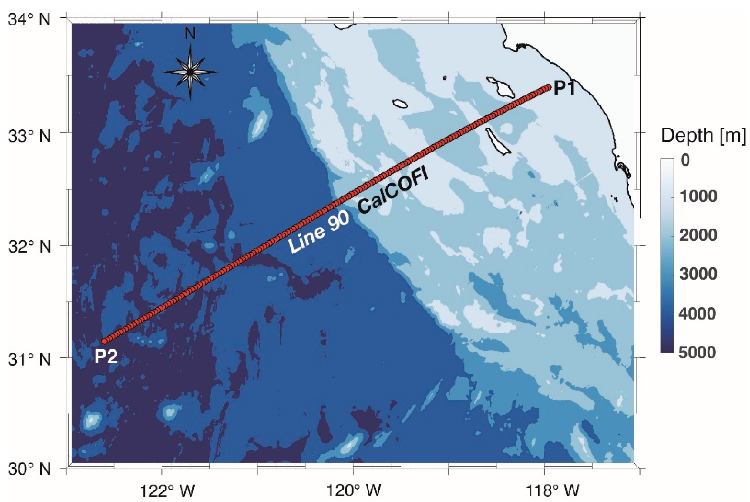
2.1. Observational Data

2.1.1. Glider Data

The data used in this work are a subset of the historical datasets gathered by the CUGN [27] with underwater gliders (Spray glider, https://spray.ucsd.edu, accesed on 22 May 2019). These autonomous vehicles employ variable buoyancy for diving and wings to glide horizontally and perform a sawtooth trajectory through the water column [27,28]. CUGN Spray gliders are equipped with a SeaBird 41CP pumped Conductivity-Temperature-Depth (CTD) sensor to measure pressure, temperature, and conductivity (salinity). Potential density (σ_θ) is computed from absolute salinity (S_A) and conservative temperature (θ) using the Thermodynamic Equation of Seawater-2010 (TEOS-10) MATLAB (https://www.mathworks.com, accessed on 23 August 2021) package.

Spray gliders can perform multiple dives from the surface to a depth of 500 m over several months, completing a cycle in 3 h while traveling less than 3 km horizontally during each dive [20]. We used a total of 70 backward and forward trajectories along the CalCOFI Line 90 (Figure 1), conducted continuously from October 2006 to December 2013. Line 90 extends from ~25 km to ~500 km offshore, that is, between locations P1 (122.59°W, 31.12°N) and P2 (117.95°W, 33.33°N).

The resolution of the glider measurements is a function of the sensor sampling frequency and glider speed. The vertical profiles are vertically averaged (grouped) at 10 m intervals from the surface to 500 m depth. However, we only used conservative temperature and potential density data from the upper 10 m for comparison with SST satellite data. Horizontally equidistant along-track measurements were obtained using a third-order polynomial function fitted to irregularly distributed glider locations along each trajectory Equation (1). The longitudes (x_i) corresponding to evenly spaced (3 km) locations between P₁ and P₂ were computed as dx = 3|P₁(1) − P₂(1)|/3 dist(P₁,P₂). These coordinates (x_i) are replaced in the fitted polynomial function to obtain the adjusted latitudes (y_i). The best-fit function obtained was a cubic polynomial of the following form:

$$f\left(x_i\right)=a_0+a_1{x}_i+a_2{x}_i^2+a_3{x}_i^3,$$

(1)

where x_i (i = 1, 2, …, N) are the longitudes of the N positions along the trajectory and a₀, a₁, a_2, a₃ are the fitted coefficients for a given trajectory. Equation (2) calculates the shortest distance between the glider position and the straight line joining P₁ and P₂. Once the coordinates are obtained for the f (x_i) = 1, 2, 3... M points, the measured SST value closest to the line (i.e., the shortest Euclidean Distance, D_E) is obtained as follows:

$$D_E\left[\left(x_i,y_i\right);\left(x_f,y_f\right)\right]=\sqrt{{\left(x_i-x_a\right)}^2+{\left(y_i-y_a\right)}^2},$$

(2)

which measures the distance to the adjusted points (x_a,y_a) in km. Finally, data values for each trajectory were organized in a matrix containing temperature and density values, distance, and date.

2.1.2. MUR Observations

Global SST images from the Multi-scale Ultra-high Resolution (MUR) data product (http://mur.jpl.nasa.gov, accessed on 30 May 2019) were used for this study to compare fronts identified using in situ glider data and fronts detected from remote satellite observations [29]. These daily, cloud-free, 1-km spatial resolution images combine measurements from various satellites (microwave and infrared) and in situ observations. These images of SST Level 4 are optimally interpolated on a global 0.01-degree grid using wavelets as basic functions. A total of 2647 images acquired between October 2006 and December 2013 were used in this study.

2.2. Front Detection

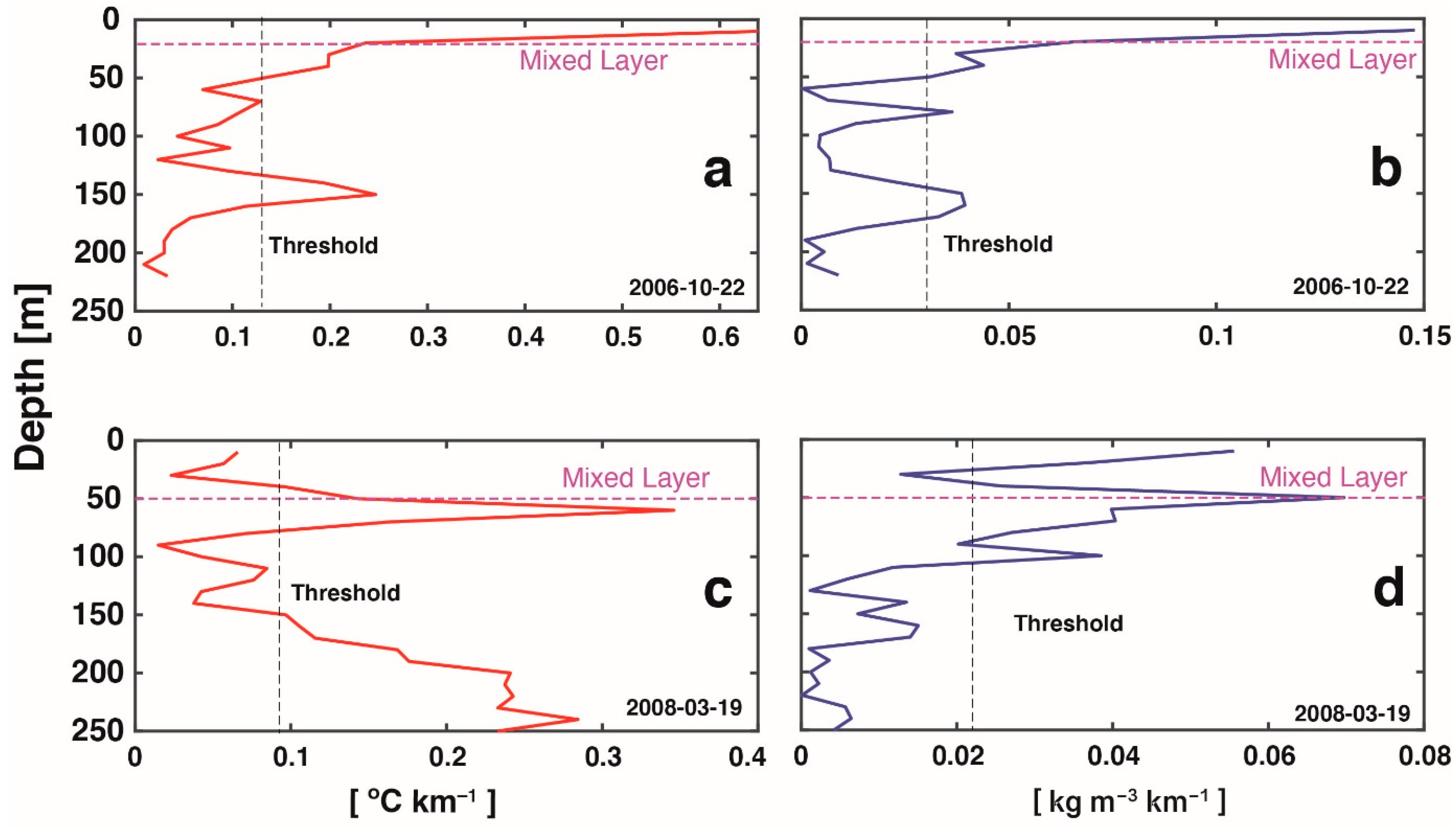
2.2.1. Front Detection with Glider Data

A gradient-based algorithm [30] was used to identify frontal zones from conservative temperature (θ fronts) and potential density (σ_θ fronts) along the glider trajectory. Along-track gradients were computed using central differences and forward/backward differences [31] at locations P₁ and P₂. The following methodology was implemented to detect frontal structures along the glider trajectory. First, glider trajectories were partitioned into three differentiated dynamical zones [15,21,24]: coastal (0–100 km offshore), transitional (100–300 km offshore), and oceanic (>300 km from the coast). Second, for each zone, a cumulative histogram of the horizontal gradients of 10-m surface-layer conservative temperature (or potential density) was computed over the study period (Figure 2). Then, a threshold was defined for each zone as the value with a gradient magnitude greater than or equal to 90% of the cumulative frequency [10,30,32,33]; this encompasses a relatively small proportion of the distribution and includes the highest gradient values observed (Figure 2). Finally, any θ-gradient whose value was greater than or equal to the threshold was identified as the edge of the front. When consecutive θ-gradients exceeded the threshold, the frontal interface was detected by selecting the location of the largest gradient.

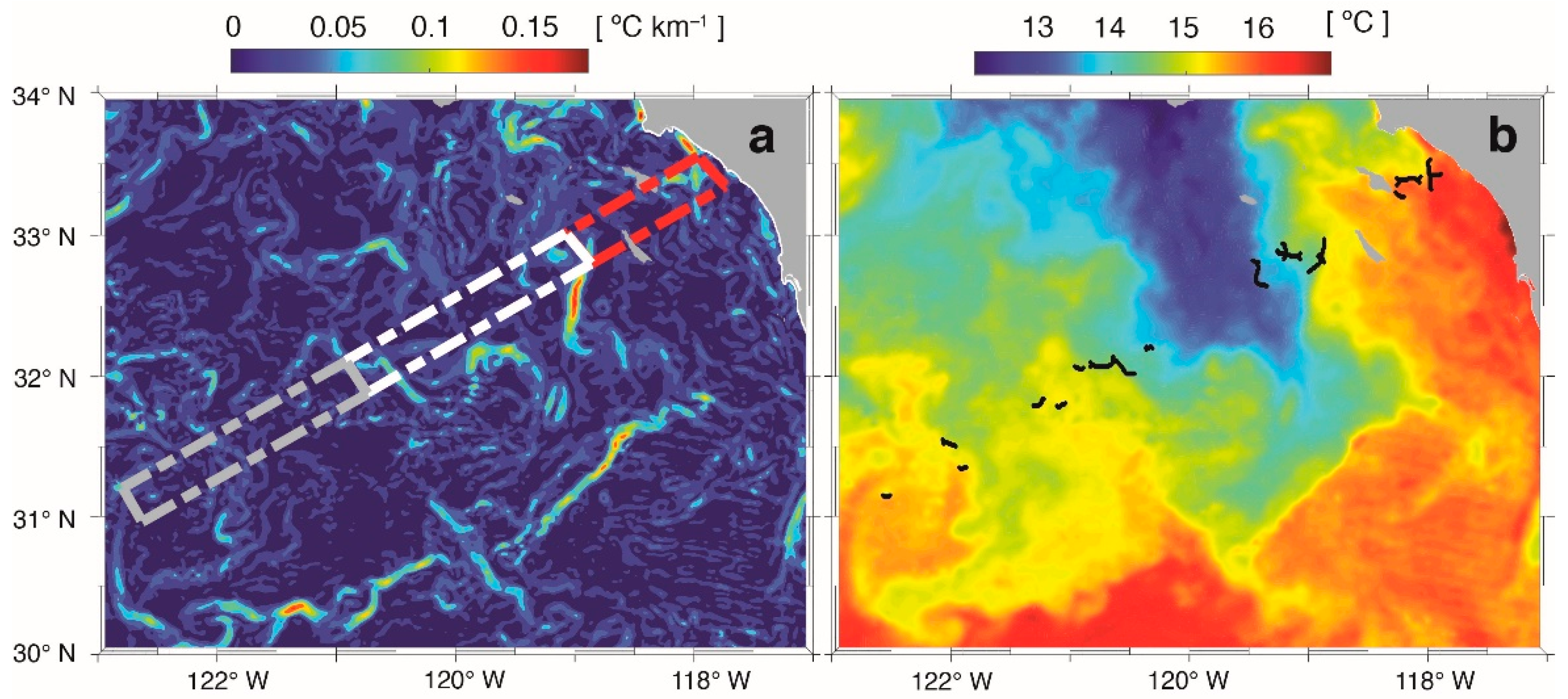
2.2.2. Front Detection with MUR Data

Two front detection methods were developed with MUR data. The first (MUR1D) consisted of interpolating the SST data to the coordinates of each glider trajectory during the study period. Thus, we obtained a new SST dataset fully comparable with in situ θ. The methodology described in Section 2.2.1 was applied to obtain the frontal structure with MUR1D. For the second method (MUR2D), the Sobel gradient operator was used to estimate the magnitude of the SST gradient in the images [34] since it allows to highlight this characteristic of the ocean effectively [18,35,36]. The Sobel operator convolves two 3 × 3 matrices or kernels with the SST image as follows:

$$Gx=\left|\begin{array}{ccc}-1& 0& 1\\ -2& 0& 2\\ -1& 0& 1\end{array}\right|\ast \mathrm{SST}; Gy=\left|\begin{array}{ccc}-1& -2& -1\\ 0& 0& 0\\ 1& 2& 1\end{array}\right|\ast \mathrm{SST},$$

(3)

where SST is the MUR data, Gx and Gy are two images that contain approximations for derivatives in horizontal and vertical directions, and * indicates the convolution operator. Then, the magnitude of the SST gradients (GM) were calculated as follows:

$$\left|G\right|=\sqrt{G{x}^2+G{y}^2}.$$

(4)

We built masks delimiting the three zones of interest: coastal (~44 km²), transitional (~49.43 km²), and oceanic (~49.64 km²), described in Section 2.1 and represented in Figure 3a. The daily SST gradients were computed using Equation (5) (Figure 3a) for each zone. SST gradients obtained during the study period were gathered on a cumulative histogram, and a threshold value was computed following the same procedure as for the glider θ-gradients. Pixels with SST gradient intensity above the threshold correspond to a frontal zone. Images were converted into binary data, i.e., 0 (negative detection) or 1 (positive detection). Pixels that are connected were grouped and indexed with a unique label. This labeling is a fundamental processing step to differentiate frontal structures from each other [37]. When consecutive frontal points with the same label value were found, the location of the maximum SST gradient was used to define the front location

2.3. Front Frequency

Once the binary matrix (zeros and ones) of the frontal detection was constructed on each grid point of the transect (3 km resolution), the Front Frequency (FF) was also computed [15] for both CUGN (θ fronts and σ_θ fronts) and MUR (MUR1D and MUR2D) datasets. Thus, FF can be interpreted as the probability of detecting a front along the (70) glider trajectories, expressed as follows:

$$\mathrm{FF}=\frac{{{\displaystyle \sum }}_{i=1}^n{N}_F}{N_T}\times 100,$$

(5)

where N_F is the number of fronts detected, and N_T is the total number of trajectories. FF values obtained for each point during the study period were averaged per zone every ~20 km from the coast to the open ocean. Bimonthly climatologies were also constructed with the FF obtained for the in situ and satellite data sets.

2.4. Thermohaline Compensation in Density and Temperature Fronts

Thermohaline density-compensated fronts can be detected following the methodology introduced by Mauzole et al. [38]:

$$C_i=r.\frac{\alpha \left|\nabla \mathrm{SST}\right|}{\left|\nabla \rho \right|},$$

(6)

where C_i is the compensation index, α is the thermal expansion coefficient, $\nabla \mathrm{SST}$ is the θ gradient, $\nabla \rho$ is the σ_θ gradient, and r (10³) is a constant introduced to obtain values of C_i = 1, corresponding to the case of non-compensation. Equation (6) was calculated in the mixed layer [39] at ~3 km before and after each temperature (θ) front detected. There are three cases concerning the values obtained from C_i:

• C_i = 1: no thermohaline compensation;
• C_i > 1: partial thermohaline compensation;
• C_i >> 1: total thermohaline compensation.

3. Results

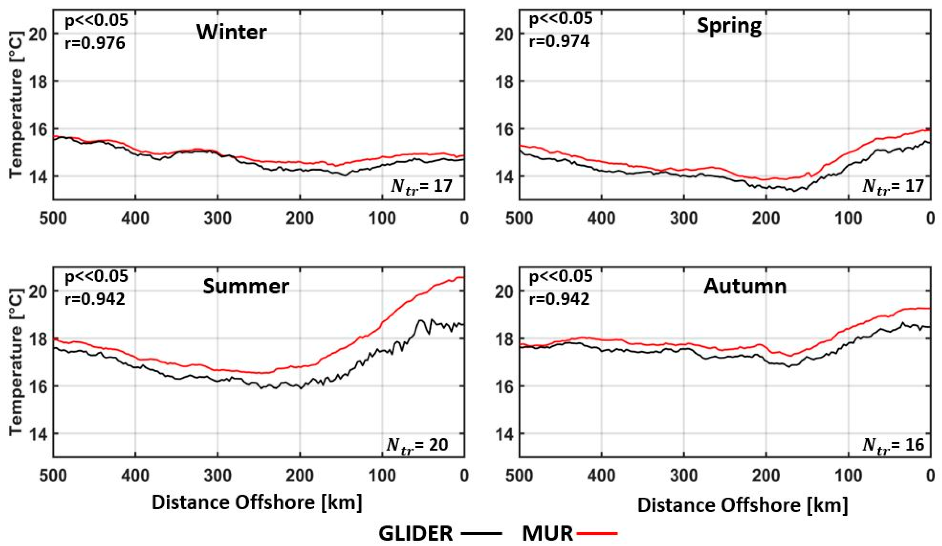
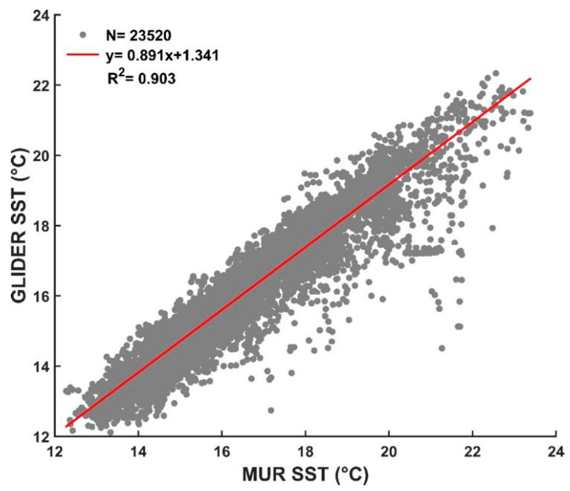
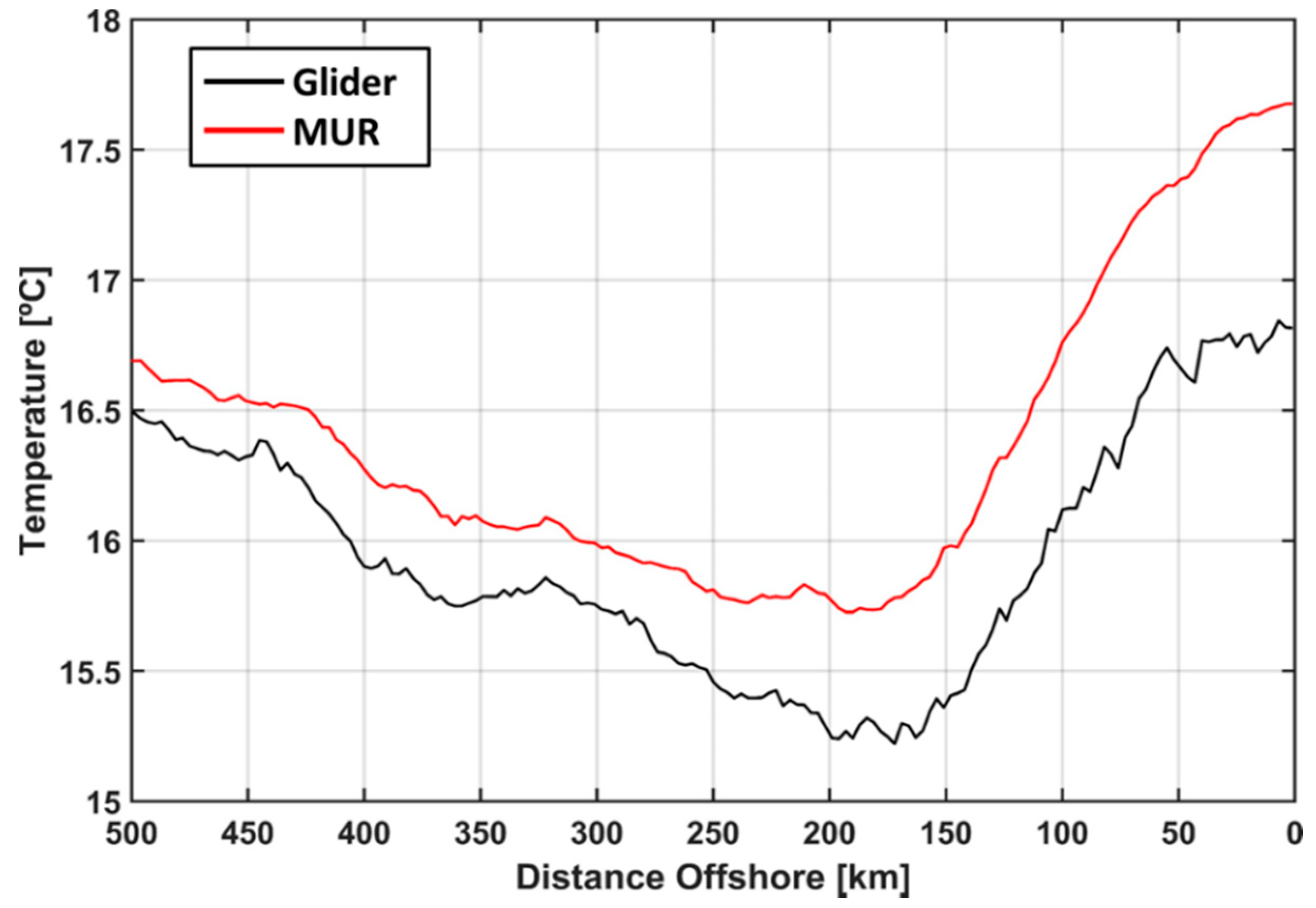
3.1. Similarity between Potential Temperature and SST

A comparison of the SST values derived from the two datasets (θ and SST) along the 70 trajectories showed a high linear Pearson’s correlation coefficient (R = 0.95) and a root mean squared error (RMSE) of 0.77 °C (Figure 4). The agreement between in situ glider and remote satellite datasets suggests that both estimates of SST across the study area are robust and contain a similar variability. The linear regression shows an intercept at 1.34 °C and R² = 0.903. The constant difference of 1.34 °C between the two datasets is related to (i) the differences between observational platforms and sensors used to measure the upper ocean temperature (i.e., thermistor vs. radiometer, satellite vs. in situ, etc.) and (ii) the differences between the depth of measurements.

The mean θ and SST, computed from the glider and MUR datasets as a function of offshore distance, also show a good agreement (Figure 5). The difference in RMSE between the two mean temperatures is 0.81 °C, with the largest differences (0.86 °C) occurring near the coast (0–50 km) and the smallest (0.2 °C) occurring offshore (near 500 km). The averaged SST is always higher than the averaged computed from in situ glider data, mainly due to differences in the depth of the measurements used to compute the mean. Both the averaged θ and SST show a similar trend along the CUGN Line 90. Near the coast (0–50 km), the mean temperature decreases smoothly at 0.006 °C km⁻¹. Between 50 and 150 km, the mean temperature decreases rapidly (0.016 °C km⁻¹), reaching a minimum near 150–200 km offshore that matches the location of the core of the California Current, which shows its maximum seasonal variability in this zone [21]. Beyond 200 km, mean temperatures increase towards the open sea but at a smaller rate (~0.003 °C km⁻¹) than the one recorded between the coastal and transition zones. Monthly means showed a high correlation (R² = 0.865, p < 0.05, RMSE = 0.485 °C) and similar seasonal variations (Figure A1), with a more pronounced decrease in θ and SST in spring near 150–200 km offshore.

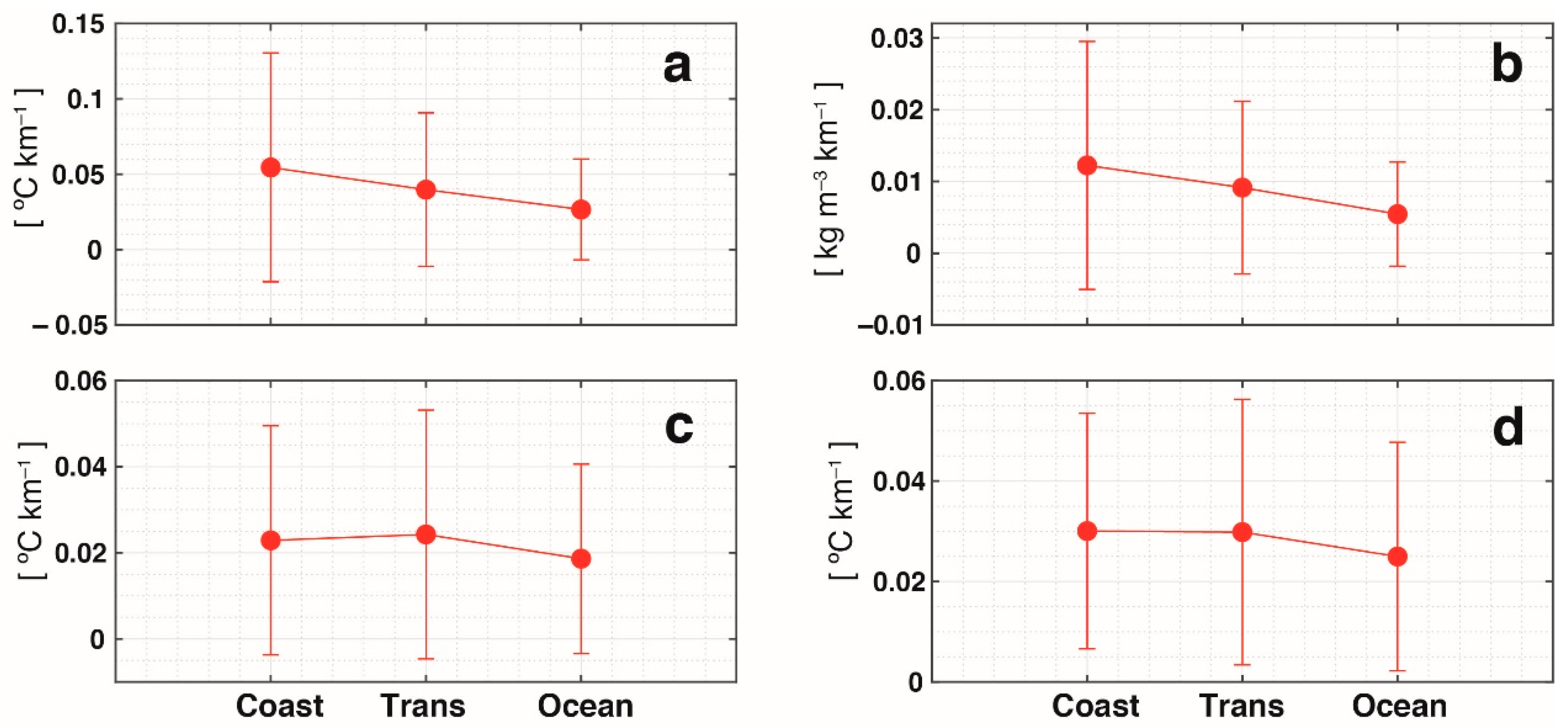
3.2. Temperature Gradients

Our front detection method is based on temperature (θ and SST) and potential density gradients (see Section 2). Capturing most of the gradient variability is essential for accurate front detection. Figure 6 shows the comparison between average θ, SST, and σ_θ gradients for each of the study areas along Line 90 using both glider and MUR data. Despite exhibiting large standard deviations, there were significant differences (p < 0.05, Kruskal–Wallis) between the averaged θ and SST gradients obtained from the two datasets for the three zones along each trajectory. In the coastal zone, the average θ gradient from the glider data is greater (~0.05 °C km⁻¹, Figure 6a) than those obtained with the MUR1D (~0.02 °C km⁻¹, Figure 6c) and MUR2D (~0.03 °C km⁻¹, Figure 6d) data. This is consistent with the higher threshold obtained for the glider data (see

Table 1. Thresholds for values obtained from conservative temperature, potential density, and sea surface temperature (SST) gradients computed from California Underwater Glider Network (CUGN) and the Multi-scale Ultra-high Resolution (MUR) datasets for the three study zones.

Zone	θ Gradients [°C km−1]	MUR1D [°C km−1]	MUR2D [°C km−1]	σθ Gradients [kg m−3 km−1]
Coastal	0.13	0.05	0.06	0.03
Transition	0.09	0.05	0.05	0.02
Offshore	0.06	0.04	0.04	0.01

). Using the glider data, three different zones are observed, identified in both the θ and σ_θ gradients, being more intense and with greater variability in the coastal zone (0 to 100 km), where the CCS upwelling system is prone to baroclinic instabilities, driving strong mesoscale and sub-mesoscale activity. Note that the offshore decrease in the mean gradient intensity is consistent with the decrease in the threshold (see Table 1). Using MUR1D and MUR2D (Figure 6c,d), the greatest variability is found toward the transition zone (100 to 300 km).

3.3. Front Detection

The persistence of fronts, or FF, is important for biogeochemical processes, as any front that lingers for a significant period of time may be associated with upper ocean convergence and accumulation of high biological productivity [40]. Figure 7 shows the typical distribution of FF along Line 90 as determined from CUGN (θ fronts and σ_θ fronts) and MUR SST (MUR1D and MUR2D) datasets. With the glider data, θ fronts and σ_θ fronts depict FF peaks in the coastal zone, located approximately at 100 km, with FF of 8.81 and 8.33, respectively. SST peaks for MUR1D and MUR2D coincide in the first 20 km near the coast, with high variability in the case of MUR1D (4.58 standard deviations). In the transition zone, the peaks of FF in θ fronts, σ_θ fronts, and MUR2D are approximately 134 km from the coast. MUR2D matches the glider data FF peaks but with high variability (3.5 standard deviations). In the case of MUR1D, the peak of FF is located at 153 km with a standard deviation of 3.18. There were two FF peaks in the θ front and σ_θ front data in the oceanic zone, the first at approximately 305 km, which coincides with MUR1D, and the second near 400 km. For MUR2D, a peak of FF was found at 381 km in the oceanic zone, with a mean and standard deviation of 5 and 3.58, respectively.

To compare the frontal detections obtained from the two datasets, a bimonthly climatology of FF for the study period was constructed to compare the frontal detections obtained from the two datasets (Figure 8). Differences in FF are noticeable, with FF peaks between July and August in the estimates based on the CUGN dataset (θ fronts and σ_θ fronts), and between November and December in those based on the MUR dataset (MUR1D SST and MUR2D SST). The CUGN climatology of FF suggests that the front frequency follows a seasonal cycle with maxima occurring in summer. In contrast, using MUR climatology of FF shows that FF increases towards autumn.

In total, 703 θ fronts and 653 σ_θ fronts were obtained from the glider data, with ~62% of θ fronts matching σ_θ fronts. The oceanic region, characterized by a deeper mixed layer (~42 m) compared to the coastal (~15 m) and transition (~26 m) zones, has, on average, a higher compensation index and a high percentage of fronts that are partially compensated (

Table 2. Averaged thermohaline density compensation index and mixed layer depth over all fronts detected using the CUGN datasets of potential density and conservative temperature for the three study zones.

Zone	Average Compensation	No Compensation [%]	Partial Compensation [%]	Mixed-Layer Depth [m]
Coastal	1.06	70	30	15
Transition	1.11	56	44	26
Offshore	1.38	39	61	42

). On the other hand, the coastal zone presents the highest number of non-thermohaline-compensated θ fronts. In general, temperature fronts that coincide with density fronts do not exhibit thermohaline compensation.

4. Discussion

4.1. Interpretation of Front Detection in the CCS

We proposed and tested, for the first time, a front detection method that applies SST image processing techniques to more than seven years of conservative temperature and potential density data collected using underwater gliders off the Southern California coast. Our method analyzes cumulative histograms of temperature gradients to define a threshold used to discriminate between frontal and non-frontal observations. The threshold is computed for three different zones (coastal, transitional, and oceanic), and its values reveal marked differences among the zones, both when using CUGN (temperature and density) and MUR2D (SST) datasets. This coincides with the work of Lynn and Simpson [21], who found different physical characteristics between coastal, transitional, and oceanic zones. The largest gradients (and thresholds) are obtained in the coastal zone from the CUGN dataset. This finding suggests that frontogenesis is enhanced near the coast, leading to the intensification of horizontal gradients and driving stronger fronts.

Some peaks in the FF distribution computed from the CUGN and MUR datasets were in agreement in some areas. These areas are highly influenced by strong physical and biological interactions [21]. The peaks in FF in the coastal zone evidenced using the CUGN dataset but barely seen using the MUR dataset likely correspond to periods of intense upwelling resulting from persistent strong equatorward wind stress and a negative wind stress curl [18,41]. The FF peaks and troughs in the transitional zone are largely driven by the interaction between mesoscale energetic meanders and eddies that interact with the core of the California Current [21]. Given the large spatial and temporal variability in the transitional zone imprinted by the mesoscale, the FF peaks observed in both CUGN and MUR datasets suggest the persistence of the Ensenada Front [15]. This front is characterized by smooth surface horizontal gradients in physical, chemical, and biological oceanographic variables and is formed by a complex set of currents, some of which feed eddies [42].

The seasonal maxima in FF obtained from the CUGN datasets are consistent with stronger (weaker) gradients of dynamic ocean height occurring in spring and summer (winter) [21]. Similar consistencies were found between the bimonthly climatology of FF obtained using the CUGN datasets and the results obtained by Castelao et al. [18], who detected ocean fronts in the CCS analyzing four years of SST imagery and found the highest FF in summer (July–August) and the lowest in winter (January–February).

4.2. Differences in Front Detection with CUGN and MUR Datasets

Although the results obtained with CUGN and MUR are consistent to some extent (see Section 4.1), large discrepancies are also evidenced. In particular, the MUR datasets provide weaker temperature gradients relative to the CUGN datasets, which leads to a weaker coastal FF. This finding contrasts with Oram et al. [10], who found frontal SST gradients between 0.15 and 0.3 °C km⁻¹ in this region. In our study, such values were attained only when in situ temperature glider data were used. In addition, the bimonthly FF obtained with MUR datasets (MUR1D and MUR2D) showed the largest FF towards the autumn, which is not consistent with the work of Castelao et al. [18], although both analyses are based on satellite SST images. This discrepancy supports the idea that the actual front dynamics is captured by CUGN but not by MUR datasets. To explain the discrepancies obtained with the two datasets, the differences in these methodological approaches are discussed below.

4.2.1. Temperature Sampling Depth

The MUR temperatures have been shown to present a warm bias compared to the glider data. This is because satellite SST data provide temperatures within the first meter of the water column (skin layer), which are usually warmer than the surface layer. In addition, horizontal SST gradients within the skin layer are highly sensitive to surface thermohaline-modifying processes such as surface heat fluxes (cooling/heating) and wind and wave mixing that mask front detection. On the contrary, the glider data overcome this limitation by averaging the temperature over the uppermost 10 m of the water column.

4.2.2. Gradient Computation

The FF estimated using MUR2D is computed from 2D horizontal gradients over the whole North Pacific Ocean off southern California. This differs from glider data, which only provide along-track θ and σ_θ gradients, thus severely limiting this method. Being approximately perpendicular to the coast, the glider data along the CUGN Line 90 captures only cross-shore gradients, while the alongshore gradients are dramatically underestimated. The MUR data were also processed to conserve only the along-track SST gradients (MUR1D) to eliminate this difference.

Table 3. Comparison (Kruskal–Wallis test) of 20-km mean front frequency (FF) values estimated using the CUGN and MUR datasets for each of the three study zones. ${\mathcal{X}}^2$ indicates the value of the Pearson’s Chi-square test, while p-Value represents the level of statistical significance. Asterisks denote significant differences (p < 0.05). θ and σ_θ fronts refer to fronts identified using conservative temperature (°C) and potential density anomaly (kg m⁻³). MUR1D and MUR2D indicate the two front detection methods used here, the interpolation of SST data to the geographical coordinates of each glider trajectory to detect fronts, and the use of the Sobel gradient operator to estimate SST gradients, respectively.

FF/METHODS	COAST		TRANSITION		OCEAN
	${\mathcal{X}}^2$	p-Value	${\mathcal{X}}^2$	p-Value	${\mathcal{X}}^2$	p-Value
θ fronts, σθ fronts, MUR1D and MUR2D	4.15	0.245	5.16	0.161	13.14	0.004 *
θ fronts and σθ fronts	0.53	0.467	0.56	0.452	0.32	0.5702
θ fronts and MUR1D	0.33	0.563	0.95	0.331	1.66	0.1974
θ fronts and MUR2D	3	0.083	2.98	0.084	10.1	0.001 *
σθ fronts and MUR1D	0.33	0.563	0.16	0.691	0.17	0.677
σθ fronts and MUR2D	2.55	0.112	2.99	0.084	6.63	0.010 *
MUR1D and MUR2D	1.33	0.248	2.83	0.092	7.03	0.008 *

shows a statistical comparison (Kruskal–Wallis test) of 20-km mean FF values computed using the CUGN and MUR datasets for each of the three zones. No differences were evident in the transitional and coastal zones, and the null hypothesis could not be rejected. However, there was a significant difference (p < 0.05) between MUR2D and the FF values obtained using the CUGN datasets in the oceanic zone. In this zone, there are significant differences (p < 0.05) between MUR1D and MUR2D, while the results using the MUR1D and CUGN datasets are similar in the oceanic zone. These differences between MUR and CUGN are related to the unsolved alongshore SST gradients in the glider data. Notice, however, that the FF estimated using the MUR1D datasets is not as large as the FF computed from the CUGN datasets. This is related to the weaker temperature gradient in the MUR datasets.

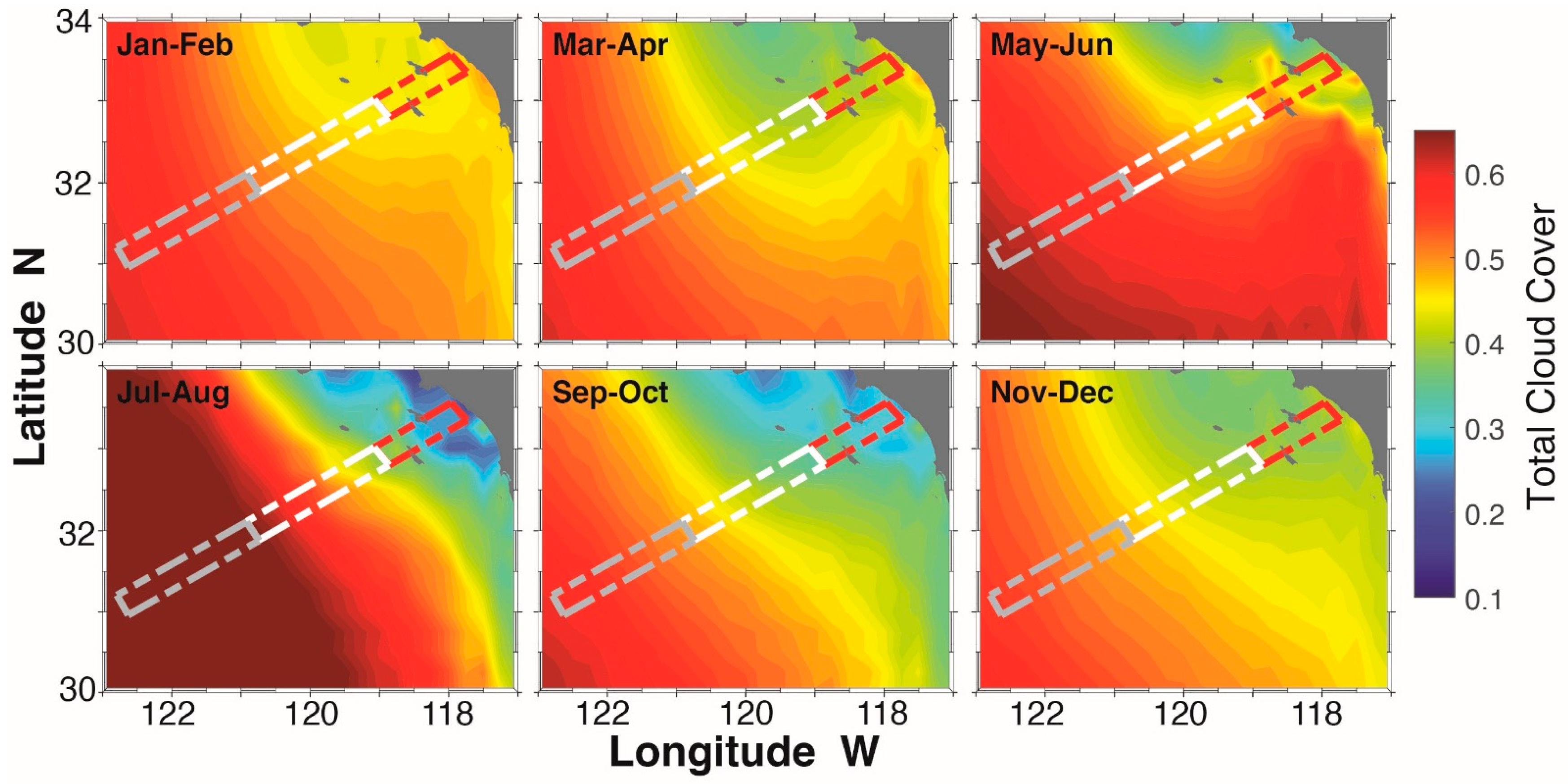
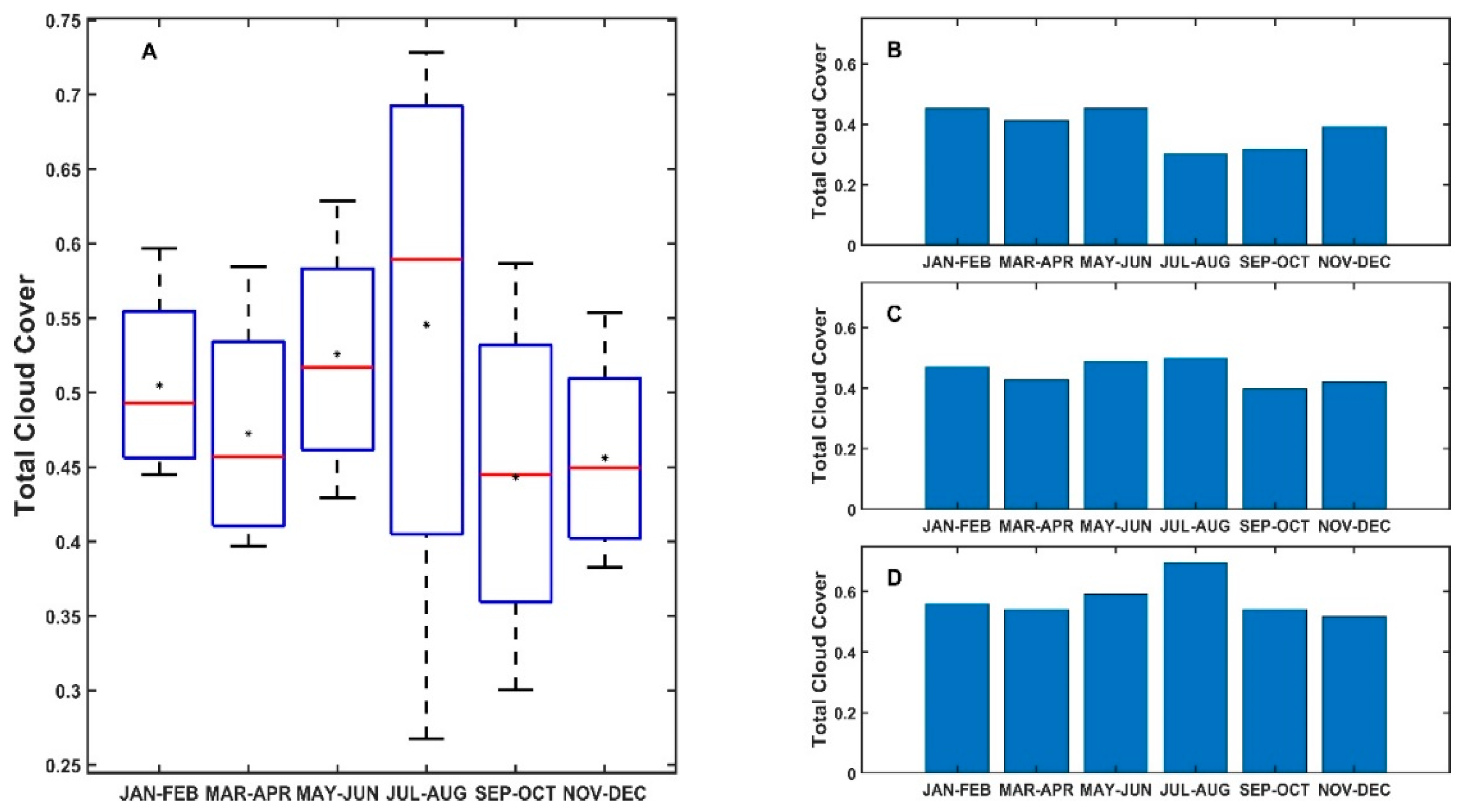
4.2.3. Cloud Cover in MUR Data

The weaker temperature gradients in MUR are consistent with the smoothing (interpolation) procedure used to obtain 2D SST images onto a regular grid and to reconstruct the SST images during periods of severe cloud cover in MUR [43]. Indeed, the MUR2D product is a blend of satellite and in situ data interpolated onto a 1 km × 1 km grid through optimal interpolation in space or time to fill gaps where no data are available. In the presence of clouds, only data from microwave radiometers (which have low spatial resolution) and in situ data (if available for that day) are optimally interpolated, leading to a smoothed SST field compared to areas with no cloud cover. This can be observed when comparing the SST gradients reported in McClatchie et al. [23], detected with the Sobel gradient operator in level-2 images with MUR2D SST gradients (Figure A3). On the contrary, gliders provide in situ, along-track high-resolution data regardless of cloud conditions. The cloud cover limitation in MUR becomes critical when selecting detection algorithms since, in addition to detecting extreme gradients, the algorithm should not be overly sensitive to the noise caused by missing data to avoid false detections.

To explain the difference in the FF of climatological cycles from the MUR and glider data, a 20-year climatology of the total cloud cover distribution in the North Pacific Ocean off southern California (Figure A2) suggests that the offshore (oceanic) zone of CUGN Line 90 is largely covered by clouds most of the year, especially in July to August. In contrast, the coastal zone has the largest cloud cover during January to February. This might explain the low FF computed using the MUR datasets in summer (winter) in the oceanic (coastal) zones (Figure 7 and Figure 9).

4.2.4. Advantages and Disadvantages of Detecting Fronts from MUR and Glider Datasets

Satellite SST data have worldwide coverage and thus offer the advantage of being available with a large spatio-temporal range, avoiding the need to conduct in situ expensive (time and money) campaigns. In addition, they allow computing 2D SST gradients. However, their resolution is considerably reduced in cloudy areas where infrared radiation cannot be measured. In these areas, the spatial smoothing generated by the MUR optimal interpolation reduces the value of spatial temperature gradients. Glider observations, by contrast, provide a high-resolution but challenging dataset that convolves spatial, temporal, or spatio-temporal variability as the glider moves along the CalCOFI Line 90. In addition, glider data provide vertical profiles. Thus, they allow cross-track front detection in deeper layers and the study of the vertical structure of fronts (Figure 10). Our method presented in this paper can be easily applied to other depths.

4.3. Sensitivity of the Results to the Front Definition

Our results rely on the definition of a frontal zone. In our method, a front is defined as gradients stronger than the 90th percentile in the study area. The value of this threshold thus depends on the area studied and the time covered by the dataset used. Longer records, such as the one used in this study, provide a robust detection of frontal structures since they capture a large portion of the temporal variability in temperature (and density) gradients at a wide range of scales. It should be noted that the threshold is objectively selected as the value at the inflection point on the cumulative function of temperature gradients [44]. This was evidenced by Oram et al. [10], who used the Canny algorithm [8] to detect fronts in SST images and recommended defining upper and lower thresholds corresponding to 90% (as in our study) and 80%, respectively, in the cumulative function of SST gradients. Computing the threshold for the area studied is necessary because the SST gradient intensity is highly variable worldwide. Furthermore, the use of a fixed threshold value would imply an under- or overestimation of the number of frontal features detected if dynamical conditions change.

The use of the thresholds defined in this study plays an important role in the detection of fronts because it can define regions that are affected by various oceanographic processes. Saraceno et al. [30] applied different thresholds for six regions of the Southwestern Atlantic Ocean using SST data, where frontogenesis associated with larger-scale deformation increases the value of the SST threshold and the variability of the FF.

4.4. Differences between Temperature and Density Fronts: Thermohaline Compensation

The upper-ocean mixed layer is often characterized by thermohaline compensation. The contributions of temperature and salinity to density tend to (partially) cancel each other out [45]. Thermohaline compensation plays a central role in detecting ocean fronts from density and may explain the differences between fronts detected from SST and density data. Fronts detected with temperature gradients agree with fronts detected with density gradients when there is no thermohaline compensation [38].

In this work, it was indeed observed that most of the thermal fronts detected have no thermohaline compensation index coinciding with density fronts (Figure 11a,b). When surface temperature gradients are weak but with no thermohaline compensation, the thermal front may go undetected (uppermost value below the threshold), although the density front may sometimes be detected (Figure 11c,d). A deepening of the mixing layer has been shown to strengthen the thermohaline compensation [46]. The mixed layer is deeper in the oceanic zone in our study region, where the weakest temperature gradients are found relative to the transition and coastal zones. The coastal zone shows a shallow mixing layer where temperature contributes the most to density gradients [46], so that most of the thermal fronts detected in this region are not thermohaline compensated and are also observed in density.

5. Conclusions

We used an automated method to detect ocean fronts from continuous glider measurements and satellite imagery. The method is based on determining a threshold value for the horizontal gradients of temperature and density from a cumulative climatological function. This threshold has been computed for the three zones studied: coastal, transition, and oceanic. Three different threshold values have been obtained, depending on the particular dynamics of each zone.

FF values computed using CUGN glider data and high-resolution MUR SST images were compared, and the spatial and temporal variability along the CUGN Line 90 was analyzed. There was moderate agreement in the identification of frontal peaks in the FF distribution concerning the distance from the coast in the three regions. However, strong differences were found in the bimonthly FF probability density functions of the computed gradients, with high (low) FF in spring–summer for the glider (MUR) data. Such differences are associated with the smoothing of the MUR data resulting from the objective interpolation, the difference in the depth of measurements, and the orientation of fronts related to the glider-track direction.

The most relevant conclusions regarding front frequency in the three zones studied are as follows:

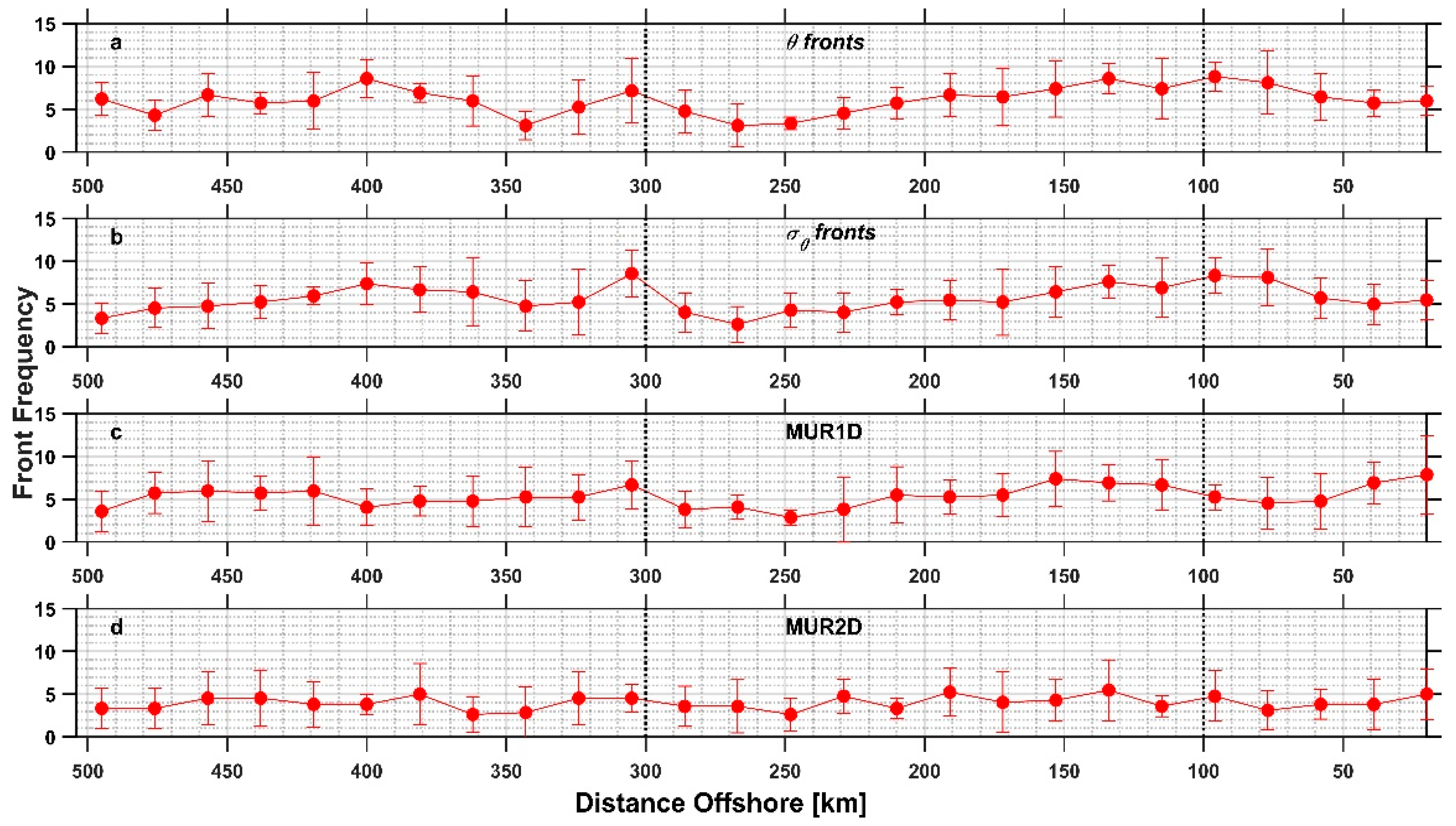
• Front Frequency (and horizontal gradients) increases significantly towards the coastal zone and in summer;
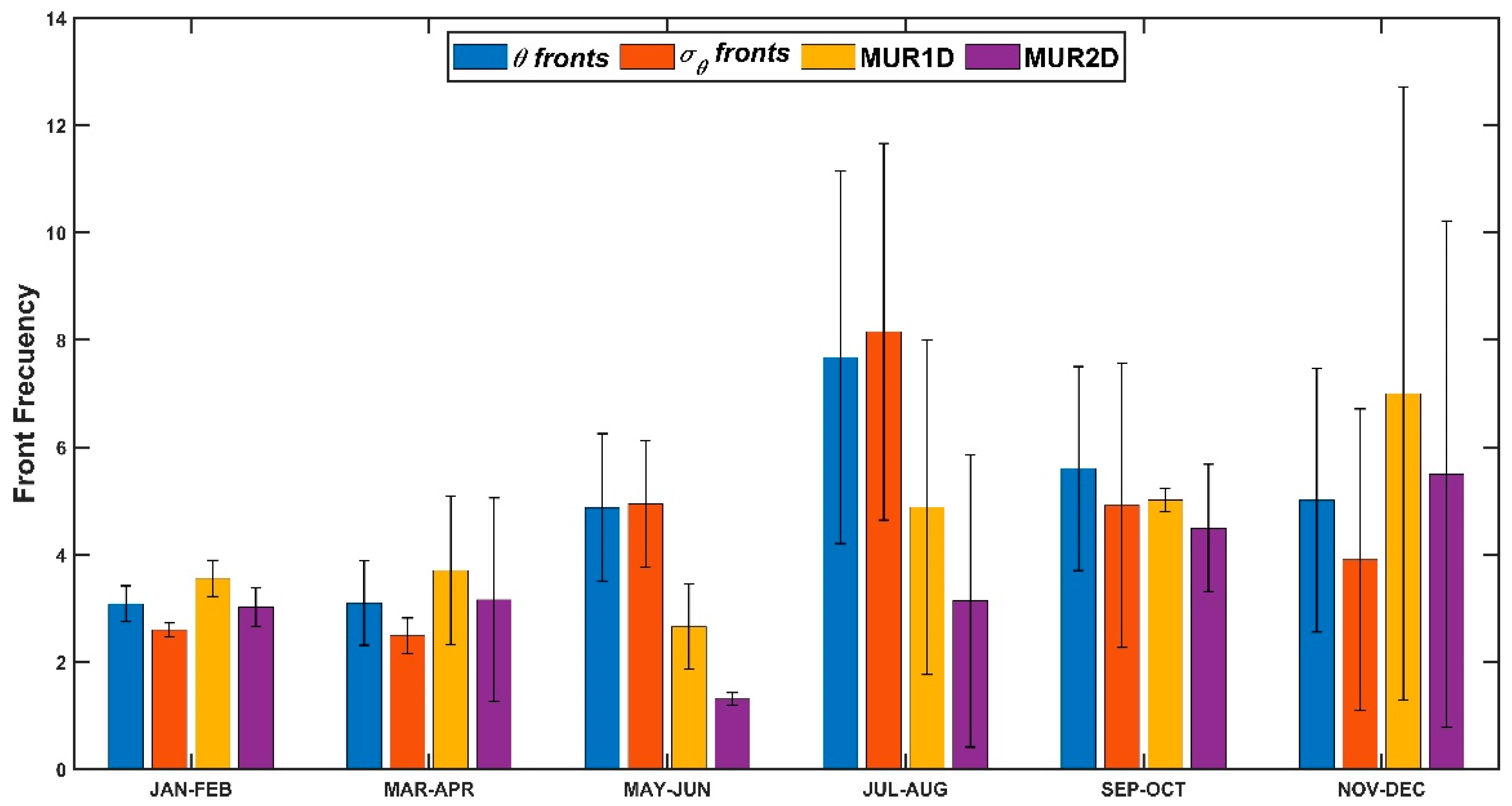
• The bimonthly climatology of FF using CUGN glider data shows a seasonal cycle, i.e., high in July–August and low in January–February, while the MUR dataset shows high FF values in November–December and low in May–June;
• The oceanic zone, distant from the CC core, exhibits the weakest horizontal gradients of the three zones, and thus fewer frontal structures are detected in this area;
• Thermohaline-compensated fronts are more abundant towards the oceanic zone, although most fronts are detected using both temperature or density criteria, indicating that the contribution of temperature to density in this region is the most important thermohaline contribution.

References

1. Ullman, D.S.; Cornillon, P.C. Satellite-derived sea surface temperature fronts on the continental shelf off the northeast US coast. J. Geophys. Res. Oceans 1999, 104, 23459–23478. [Google Scholar] [CrossRef]
2. Hoskins, B.J. The mathematical theory of frontogenesis. Annu. Rev. Fluid Mech. 1982, 14, 131–151. [Google Scholar] [CrossRef]
3. Mcwilliams, J.C.; Molemaker, M.J.; Olafsdottir, E.I. Linear fluctuation growth during frontogenesis. J. Phys. Oceanogr. 2009, 39, 3111–3129. [Google Scholar] [CrossRef] [Green Version]
4. McWilliams, J.C.; Molemaker, M.J. Baroclinic frontal arrest: A sequel to unstable frontogenesis. J. Phys. Oceanogr. 2011, 41, 601–619. [Google Scholar] [CrossRef]
5. FrankS, P.J. Phytoplankton blooms at fronts: Patterns, scales, and physical forcing mechanisms. Rev. Aquat. Sci. 1992, 6, 121–137. [Google Scholar]
6. Franks, P.J.S.; Diego, S. Sink or swim: Accumulation of biomass at fronts. Mar. Ecol. Prog. Ser. Oldend. 1992, 82, 1–12. [Google Scholar] [CrossRef]
7. Franks, P.J.S.; Walstad, L.J. Phytoplankton patches at fronts: A model of formation and response to wind events. J. Mar. Res. 1997, 55, 1–29. [Google Scholar] [CrossRef]
8. Canny, J. A Computational Approach to Edge Detection. IEEE Trans. Pattern Anal. Mach. Intell. 1986, PAMI-8, 679–698. [Google Scholar] [CrossRef]
9. Holyer, R.J.; Peckinpaugh, S.H. Edge detection applied to satellite imagery of the oceans. IEEE Trans. Geosci. Remote Sens. 1989, 27, 46–56. [Google Scholar] [CrossRef] [Green Version]
10. Oram, J.J.; McWilliams, J.C.; Stolzenbach, K.D. Gradient-based edge detection and feature classification of sea-surface images of the Southern California Bight. Remote Sens. Environ. 2008, 112, 2397–2415. [Google Scholar] [CrossRef]
11. Cayula, J.-F.; Cornillon, P. Edge Detection Algorithm for SST Images. J. Atmos. Ocean. Technol. 1992, 9, 67–80. [Google Scholar] [CrossRef]
12. Ullman, D.S.; Cornillon, P.C. Evaluation of front detection for satellite-derived SST data using in situ observations. J. Atmos. Ocean. Technol. 2000, 17, 1667–1675. [Google Scholar] [CrossRef]
13. Diehl, S.F.; Budd, J.W.; Ullman, D.; Cayula, J.F. Geographic window sizes applied to remote sensing sea surface temperature front detection. J. Atmos. Ocean. Technol. 2002, 19, 1105–1113. [Google Scholar] [CrossRef]
14. Taylor, P.; Miller, P. Multi-spectral front maps for automatic detection of ocean colour features from SeaWiFS. Int. J. Remote Sens. 2004, 25, 1437–1442. [Google Scholar] [CrossRef]
15. Kahru, M.; Lorenzo, E.D.I.; Manzano-sarabia, M.; Mitchell, B.G.; Di Lorenzo, E.; Manzano-sarabia, M.; Mitchell, B.G. Spatial and temporal statistics of sea surface temperature and chlorophyll fronts in the California Current. J. Plankton Res. 2012, 34, 749–760. [Google Scholar] [CrossRef] [Green Version]
16. Nieto, K.; Demarcq, H.; McClatchie, S. Mesoscale frontal structures in the Canary Upwelling System: New front and filament detection algorithms applied to spatial and temporal patterns. Remote Sens. Environ. 2012, 123, 339–346. [Google Scholar] [CrossRef]
17. Shimada, T.; Sakaida, F.; Kawamura, H.; Okumura, T. Application of an edge detection method to satellite images for distinguishing sea surface temperature fronts near the Japanese coast. Remote Sens. Environ. 2005, 98, 21–34. [Google Scholar] [CrossRef]
18. Castelao, R.M.; Mavor, T.P.; Barth, J.A.; Breaker, L.C. Sea surface temperature fronts in the California Current System from geostationary satellite observations. J. Geophys. Res. 2006, 111, C09026. [Google Scholar] [CrossRef] [Green Version]
19. Send, U.; Davis, R.; Fischer, J.; Imawaki, S.; Kessler, W.; Meinen, C.; Owens, B.; Roemmich, D.; Rossby, T.; Rudnick, D.; et al. A global boundary current circulation observing network. Proc. Ocean. 09 Sustain. Ocean Obs. Inf. Soc. 2010, 2. [Google Scholar] [CrossRef] [Green Version]
20. Rudnick, D.L.; Zaba, K.D.; Todd, R.E.; Davis, R.E. Progress in Oceanography A climatology of the California Current System from a network of underwater gliders. Prog. Oceanogr. 2017, 154, 64–106. [Google Scholar] [CrossRef]
21. Lynn, R.J.; Simpson, J.J. The California Current system: The seasonal variability of its physical characteristics. J. Geophys. Res. 1987, 92, 12947. [Google Scholar] [CrossRef]
22. Davis, R.E.; Ohman, M.D.; Rudnick, D.L.; Sherman, J.T.; Hodges, B. Glider surveillance of physics and biology in the southern California Current System. Limnol. Oceanogr. 2008, 53, 2151–2168. [Google Scholar] [CrossRef] [Green Version]
23. Mcclatchie, S.; Cowen, R.; Nieto, K.; Greer, A.; Luo, J.Y.; Guigand, C.; Demer, D.; Griffith, D.; Rudnick, D. Resolution of fine biological structure including small narcomedusae across a front in the Southern California Bight. J. Geophys. Res. Ocean. 2012, 117, 1–18. [Google Scholar] [CrossRef]
24. Powell, J.R.; Ohman, M.D. Covariability of zooplankton gradients with glider-detected density fronts in the Southern California Current System. Deep. Res. Part II Top. Stud. Oceanogr. 2015, 112, 79–90. [Google Scholar] [CrossRef]
25. Todd, R.E.; Rudnick, D.L.; Mazloff, M.R.; Cornuelle, B.D.; Davis, R.E. Thermohaline structure in the California Current System: Observations and modeling of spice variance. J. Geophys. Res. Ocean. 2012, 117, 1–19. [Google Scholar] [CrossRef] [Green Version]
26. Todd, R.E.; Rudnick, D.L.; Davis, R.E.; Ohman, M.D. Underwater gliders reveal rapid arrival of El Niño effects off California’s coast. Geophys. Res. Lett. 2011, 38, 1–5. [Google Scholar] [CrossRef] [Green Version]
27. Rudnick, D.L. Ocean Research Enabled by Underwater Gliders. Ann. Rev. Mar. Sci. 2016, 8, 519–541. [Google Scholar] [CrossRef]
28. Sherman, J.; Davis, R.E.; Owens, W.B.; Valdes, J. The Autonomous Underwater Glider “Spray”. IEEE J. Ocean. Eng. 2001, 26, 437–446. [Google Scholar] [CrossRef] [Green Version]
29. Physical Oceanography Distributed Active Archive Center. JPL MUR MEaSUREs Project. 2015. Foundation Sea Surface Temperature Analysis. Ver. 4.1; Physical Oceanography Distributed Active Archive Center: Pasadena, CA, USA, 2015. [CrossRef]
30. Saraceno, M.; Provost, C.; Piola, A.R.; Bava, J.; Gagliardini, A. Brazil Malvinas Frontal System as seen from 9 years of advanced very high resolution radiometer data. J. Geophys. Res. C Ocean. 2004, 109, C05027. [Google Scholar] [CrossRef]
31. Gautschi, W. Numerical Analysis; Springer Science & Business Media: Boston, MA, USA, 1997; ISBN 978-0-8176-8258-3. [Google Scholar] [CrossRef]
32. Rivas, A.L.; Pisoni, J.P. Identification, characteristics and seasonal evolution of surface thermal fronts in the Argentinean Continental Shelf. J. Mar. Syst. 2010, 79, 134–143. [Google Scholar] [CrossRef]
33. Ping, B.; Su, F.; Meng, Y.; Fang, S.; Du, Y. A model of sea surface temperature front detection based on a threshold interval. Acta Oceanol. Sin. 2014, 33, 65–71. [Google Scholar] [CrossRef]
34. Sobel, I.; Feldman, G. “A 3×3 Isotropic Gradient Operator for Image Processing,” Pattern Classification and Scene Analysis. 1973, pp. 271–272. Available online: https://www.researchgate.net/publication/285159837_A_33_isotropic_gradient_operator_for_image_processing (accessed on 12 November 2021).
35. Belkin, I.M.; Reilly, J.E.O. An algorithm for oceanic front detection in chlorophyll and SST satellite imagery. J. Mar. Syst. 2009, 78, 319–326. [Google Scholar] [CrossRef]
36. Robinson, I.S. Discovering the Ocean from Space: The Unique Applications of Satellite Oceanography; Springer Science & Business Media: Berlin/Heidelberg, Germany, 2010; ISBN 3540683224. [Google Scholar] [CrossRef]
37. Gonzalez, R.C.; Woods, R.E.; Masters, B.R. Digital Image Processing, 3rd ed.; Prentice Hall: Upper Saddle River, NJ, USA, 2009; ISBN 978-0-13-168728-8. [Google Scholar]
38. Mauzole, Y.L.; Torres, H.S.; Fu, L.L. Patterns and Dynamics of SST Fronts in the California Current System. J. Geophys. Res. Ocean. 2020, 125, e2019JC015499. [Google Scholar] [CrossRef]
39. de Boyer Montégut, C.; Madec, G.; Fischer, A.S.; Lazar, A.; Iudicone, D. Mixed layer depth over the global ocean: An examination of profile data and a profile-based climatology. J. Geophys. Res. C Ocean. 2004, 109, 1–20. [Google Scholar] [CrossRef]
40. Bakun, A. Fronts and eddies as key structures in the habitat of marine fish larvae: Opportunity, adaptive response. Sci. Mar. 2006, 70, 105–122. [Google Scholar] [CrossRef]
41. Breaker, L.C.; Mooers, C.N.K. Oceanic variability off the Central California coast. Prog. Oceanogr. 1986, 17, 61–135. [Google Scholar] [CrossRef]
42. Haury, I.R.; Fey, C.L.; McGowan, J.A. The Ensenada front: July 1985. Calif. Coop. Ocean. Fish. Investig. Rep. 1993, 34, 69–88. [Google Scholar]
43. Vazquez-Cuervo, J.; Torres, H.S.; Menemenlis, D.; Chin, T.; Armstrong, E.M. Relationship between SST gradients and upwelling off Peru and Chile: Model/satellite data analysis. Int. J. Remote Sens. 2017, 38, 6599–6622. [Google Scholar] [CrossRef]
44. Wu, Q.Z.; Cheng, H.Y.; Jeng, B.S. Motion detection via change-point detection for cumulative histograms of ratio images. Pattern Recognit. Lett. 2005, 26, 555–563. [Google Scholar] [CrossRef]
45. Ferrari, R.; Paparella, F. Compensation and alignment of thermohaline gradients in the ocean mixed layer. J. Phys. Oceanogr. 2003, 33, 2214–2223. [Google Scholar] [CrossRef] [Green Version]
46. Rudnick, D.L.; Martin, J.P. On the horizontal density ratio in the upper ocean. Dyn. Atmos. Ocean. 2002, 36, 3–21. [Google Scholar] [CrossRef]
Figure 1. Study area: The bathymetry of the eastern Pacific Ocean off southern California is shown in colormap (https://www.gebco.net, accessed on 12 November 2020). The trajectory of a CUGN spray glider between 21 October and 12 November 2016, along the CalCOFI Line 90 is indicated with a red line. Black dots P1 and P2 refer to the starting and ending locations of the CalCOFI Line 90, respectively.
Remotesensing 13 05032 g001
Figure 2. Histograms (bars) and cumulative frequency (red line) of the along-track gradients of conservative temperature (θ) in the coastal zone for the whole study period along CUGN Line 90 (Figure 1). An upper threshold at 90% of the cumulative frequency (vertical red dashed line) was used for frontal detection. θ gradients greater than the threshold are positive detections. The same methodology was used for along-track potential density and the MUR SST series for the three study zones.
Remotesensing 13 05032 g002
Figure 3. (a) SST gradients (°C km−1) and (b) SST (°C) from MUR data on 5 May 2007. The dashed lines in Figure 3a represent coastal (red), transitional (white), and oceanic (grey) zones where oceanic fronts (black contours in Figure 3b) were detected using the MUR2D algorithm.
Remotesensing 13 05032 g003
Figure 4. Scatter plot between conservative temperature values obtained from glider at the shallowest bin (z = −10 m) and MUR SST for the whole study period. The red line is the best-fit straight line (GLIDER SST = 1.341 + 0.891 * MUR SST) for the data. N is the total number of data included in this analysis, and R2 is the squared Pearson’s correlation coefficient.
Remotesensing 13 05032 g004
Figure 5. Averaged q and SST as a function of distance from the coast (along Line 90) estimated using CUGN glider (black line) and MUR (red line) datasets for the 70 trajectories.
Remotesensing 13 05032 g005
Figure 6. (a) Averaged θ gradients (°C km−1) and (b) σθ gradients (kg m−3 km−1) computed from CUGN glider data for the three study zones: coastal (Coast), transition (Trans), and offshore (Ocean); (c) and (d) show averaged SST computed using MUR1D and MUR2D datasets, respectively. Vertical red bars indicate the standard deviation.
Remotesensing 13 05032 g006
Figure 7. Front Frequency (FF) computed using detection criteria based on (a) θ gradients and (b) σθ gradients from the CUGN dataset, and (c) SST gradients from MUR1D and (d) MUR2D datasets along the CalCOFI Line 90. Error bars refer to standard deviation, and vertical dashed lines indicate the limits of the three zones of interest.
Remotesensing 13 05032 g007
Figure 8. Bimonthly climatology of FF for the study period using CUGN (blue and red bars) and MUR datasets (yellow and magenta) along the CalCOFI Line 90 for the 70 trajectories. Error bars refer to standard deviation.
Remotesensing 13 05032 g008
Figure 9. Bimonthly climatology of total cloud cover for ERA5-derived datasets over the study period (A) and for coastal (B), transition (C), and oceanic zones (D).
Remotesensing 13 05032 g009
Figure 10. Case study for frontal detection using a CUGN dataset and θ-gradient criteria. The glider performed the detection of ocean fronts along a single trajectory (#10 of Line 90) on October 4 and 24, 2007. (a) Fronts detected along Line 90: coastal zone (red dots), transitional zone (magenta dots), and oceanic zone (cyan dots). A vertical section of conservative temperature between the surface and 250 m depth along Line 90 is shown in panel (b). Vertical dashed lines indicate the limits of the three zones studied.
Remotesensing 13 05032 g010
Figure 11. Vertical profiles of horizontal gradients of temperature (left) and density (right). The vertical black dashed line indicates the threshold obtained from the surface temperature front detection. The horizontal magenta dashed line is the mixed layer depth. (a,b) are coastal profiles; (c,d) are profiles in the transitional region.
Remotesensing 13 05032 g011