Article

Estimation of Forest Aboveground Biomass in Karst Areas Using Multi-Source Remote Sensing Data and the K-DBN Algorithm

1
School of Forestry, Nanjing Forestry University, Nanjing 210037, China
2
School of Smart Agricultural, Suzhou Polytechnic Institute of Agriculture, Suzhou 215008, China
3
School of Computer Science and Technology, Soochow University, Suzhou 215301, China
*
Author to whom correspondence should be addressed.
Remote Sens. 2021, 13(24), 5030; https://doi.org/10.3390/rs13245030
Submission received: 1 October 2021 / Revised: 28 November 2021 / Accepted: 8 December 2021 / Published: 10 December 2021

Abstract

:
Accurate estimation of forest biomass is the basis for monitoring forest productivity and carbon sink function, which is of great significance for the formulation of forest carbon neutralization strategy and forest quality improvement measures. Taking Guizhou, a typical karst region in China, as the research area, this study used Landsat 8 OLI, Sentinel-1A, and China national forest resources continuous inventory data (NFCI) in 2015 to build a deep belief network (DBN) model for aboveground biomass (AGB) estimation. Based on the introduction of forest canopy density (FCD), we improved the DBN model to design the K-DBN model with the highest estimation accuracy is selected for AGB inversion and spatial mapping. The results showed that: (1) The determination coefficients R2 of DBN is 0.602, which are 0.208, 0.101 higher than that of linear regression (LR) and random forest (RF) model. (2) The K-DBN algorithm was designed based on FCD to optimize the DBN model, which can alleviate the common problems of low-value overestimation and high-value underestimation in AGB estimation to a certain extent to improve the estimation accuracy. The maximum R2 of the model reached 0.848, and we mapped the forest AGB using the K-DBN model in the study area in 2015. The conclusion of this study: Based on multi-source optical and radar data, the retrieval accuracy of forest AGB can be improved by considering the FCD, and the deep learning algorithm K-DBN is excellent in forest AGB remote sensing estimation. These research results provide a new method and data support for the spatio-temporal dynamic remote sensing monitoring of forest AGB in karst areas.

Graphical Abstract

1. Introduction

Forest ecosystems play a key role in the terrestrial ecosystem carbon cycle, water cycle, and radiant energy exchange [1,2,3]. They are the largest carbon pools in terrestrial ecosystems and play a vital role in absorbing greenhouse gases such as carbon dioxide in the atmosphere, reducing the greenhouse gas concentration, and mitigating global climate change [4,5]. Forests are an important part of terrestrial ecosystems, which have a complex community structure, rich biodiversity, and important ecological functions. They play an extremely important and irreplaceable role in regulating the carbon balance and improving the regional ecological environment. At the same time, they are also the main topic of global climate warming research [6,7]. Forest biomass is the accumulation of dry matter produced by a forest plant community in its life process, which is expressed by the dry matter mass accumulated per unit area or per unit time, usually including the total weight of stems, branches, leaves, and roots [8]. The forest AGB used in this study was only the aboveground biomass of trees, excluding underground roots, herbs, and understory litter. It reflects the management level and utilization value of forests [9,10,11]. Therefore, accurate estimation of forest biomass is the top priority in the study of the Earth’s carbon cycle and global climate change. It plays an important role in understanding and monitoring the response of forest ecosystems to greenhouse gas emissions. It can also provide strategic guidelines for sustainable forest management and is of great significance for the rational utilization of forest resources and the improvement of the forest ecological environment [12,13,14,15].
It takes a long time and requires lots of manpower and material resources for traditional forest biomass ground survey estimation. Thus, it is difficult to measure the forest AGB in a large area in real-time by ground survey method [2,16,17]. With the development of remote sensing and information technology, scholars have begun to use remote sensing technology with ground survey data to monitor regional forest biomass. Since the Landsat series satellites were put into use in the 1970s, they have good stability and sustainability, which is very conducive to the study of long-term biomass changes. Many studies use Landsat images for long time-series forest monitoring and mapping [18,19,20]. Li et al. [21] constructed a linear forest biomass estimation model for different vegetation types and integrated the forest canopy density (FCD) using Landsat 8 OLI images and fixed the sample plot data in western Hunan. Although there are still the problems of low-value overestimation and high-value underestimation, the accuracy of forest biomass estimation has generally improved. It has been confirmed that there is a close relationship between FCD and forest biomass. Generally, the forest biomass with higher FCD is higher; on the contrary, the forest biomass with lower FCD is lower [22]. Li et al. [14] used Landsat 8 OLI images and the NFCI data to compare the performances of three algorithms of Linear regression (LR), random forest (RF), and extreme gradient enhancement (XGBoost). Compared to the LR model, the estimation accuracy (R2) of XGBoost and the RF model for the coniferous forest, broadleaf forest, and mixed forest reached more than 0.75. Optical images are usually limited by spectral reflectance saturation, resulting in the over- and underestimation of the forest biomass. Ou et al. [23] incorporated forest age as a dummy variable into the forest biomass inversion model, which improved the estimation accuracy of the AGB of a dense pine forest in Yunnan, southwest China. In Ou’s paper, the model with the age dummy variable greatly reduced the overestimation of plots with an AGB value less than 70 Mg/ha and the underestimation of plots with an AGB value greater than 180 Mg/ha.
Optical remote sensing is affected by weather, clouds, and fog, especially in mountainous areas with more clouds and fog. Spectral data are inevitably oversaturated due to sensors, illumination, and other reasons. Scholars began to explore the estimation of forest biomass in large areas based on the Polarimetric SAR and Lidar satellites [24,25,26,27,28]. Yan et al. [29] established biomass models of different forest types (coniferous, mixed, and broad-leaved forests) using NFCI, Landsat 8 OLI, and ALOS PALSAR-2 data in Beijing. The estimated value of the RF model is better than that of the multiple linear regression model (MLR), showing a higher R2 (>0.6) and a lower root mean square error (RMSE; <13.5 Mg/ha). Chen et al. [30] used Sentinel-1, Sentinal-2, and Digital Elevation Model (DEM) data to establish five evaluation algorithms: Stepwise regression (SWR), machine learning (ML), artificial neural network (ANN), regression support vector machine (SVM), and random forest (RF). It was found that the RF model performed best. Vaglio et al. [31] used ALOS PALSAR-2 and Landsat 8 OLI images to retrieve the forest biomass in two mixed forest areas, confirmed the complementarity of optical and SAR data, and found that satellite data with low cost and wide coverage can be as effective as Lidar, especially in areas with high carbon density. Chen et al. [32] used the multispectral band, vegetation index of Sentinal-2, texture features, and backscattering coefficient of Sentinel-1 to develop biomass prediction models by the geographically weighted regression (GWR) and machine learning (ML) algorithms. It was found that ML has better estimation accuracy than the linear model using 56 measured AGB samples from Changbai Mountain Center in China. Li et al. [33] used Landsat 8 OLI, Sentinel-1A images, and the NFCI data to estimate the biomass of subtropical forests in Hunan Province, China. They proved that the XGBoost model can reduce the problem of overestimation and underestimation. Ho et al. [34] estimated the forest biomass of Madagascar using the radar satellite ALOS PALSAR-2 and the optical Landsat-derived tree cover and found that the radar signal was highly correlated with the biomass (R2 = 0.71) and that the root mean square error was 30% from 2007 to 2010.
To sum up, the existing research has the following three problems: (1) Forest AGB estimation research areas are basically of the small- and medium-sized scale at the county and municipal levels. Due to the incompleteness of ground data surveys, there is little estimation of forest AGB in provincial areas or at larger areas [35,36,37]. (2) Since its light saturation, overestimation or underestimation is inevitable with forest AGB using optical remote sensing [37,38,39]. (3) In previous studies, conventional linear models or traditional machine algorithms [40,41,42], such as RF, SVM, ANN, or KNN, are mostly used for forest biomass estimation, while deep learning algorithms such as the deep belief network (DBN) are rarely used in forest biomass estimation [43,44,45]. The DBN is a deep learning model that belongs to end-to-end learning. The DBN algorithm includes several RBMs (unsupervised learning), and a BP network is added to the last layer to realize supervised learning. The key point of the DBN deep learning algorithm is the weight iterative correction between visible (V) and hidden (H), which reconstructs the input data so that these data can gradually show (filter or summarize) the feature set expressing the input data.
Karst is a special and precious landform. The karst area represented by Guizhou is a typical representative of the global karst landform, which is of typical significance for the study of the forest ecosystem of the global special karst landform [46,47]. In this study, Guizhou, also a typical karst area in China, was taken as the research area, the Landsat 8 OLI and Sentinel-1A images were collected to construct a multiple linear regression (LR) model, an RF model, and a DBN model for different forest types. Then, by introducing the FCD, the K-DBN model for biomass inversion was constructed to improve the estimation accuracy of forest biomass in the karst area. This helped to improve the estimation accuracy of forest AGB in karst areas, to provide an approach for the accurate estimation of forest carbon sinks in karst areas [44,48].

2. Data and Material
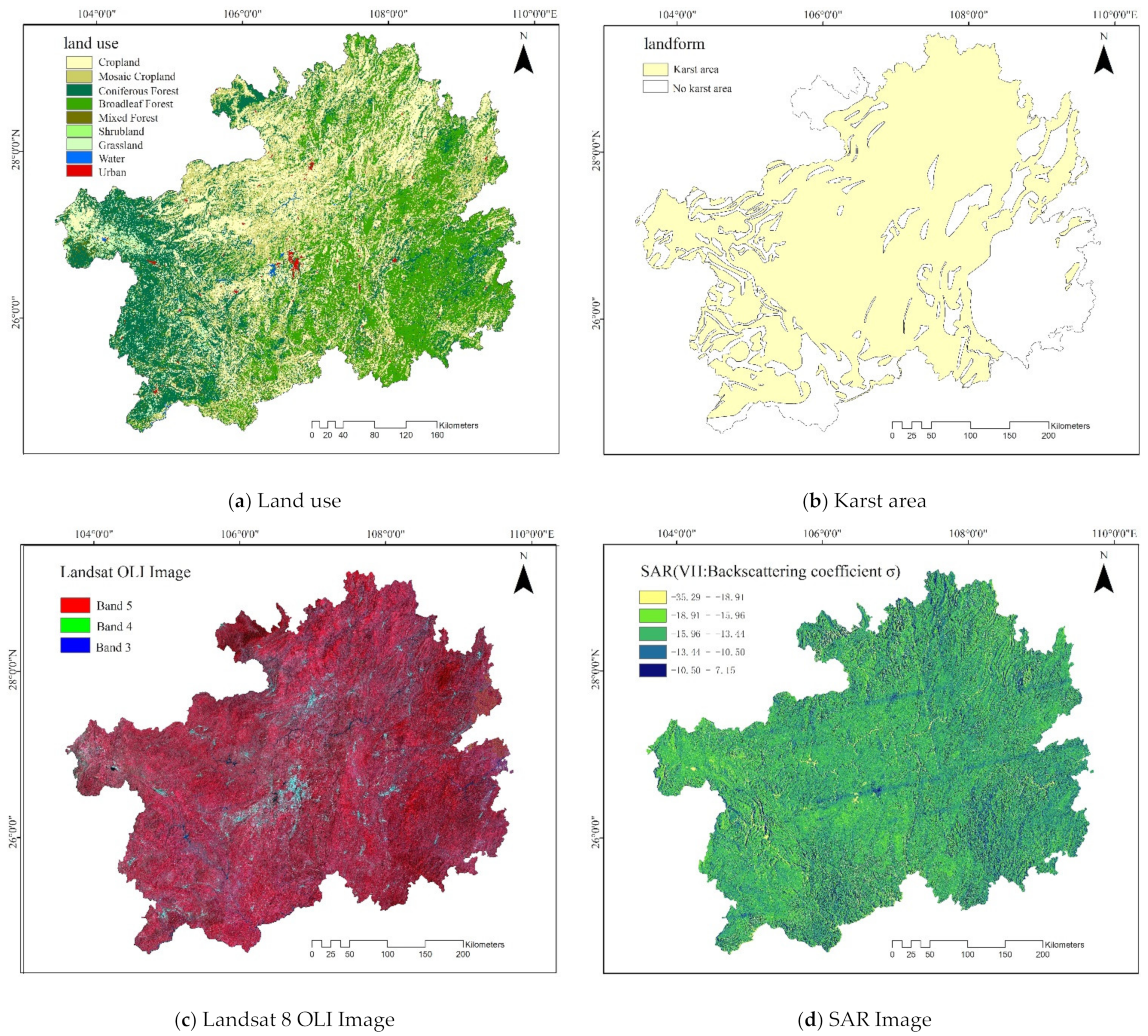
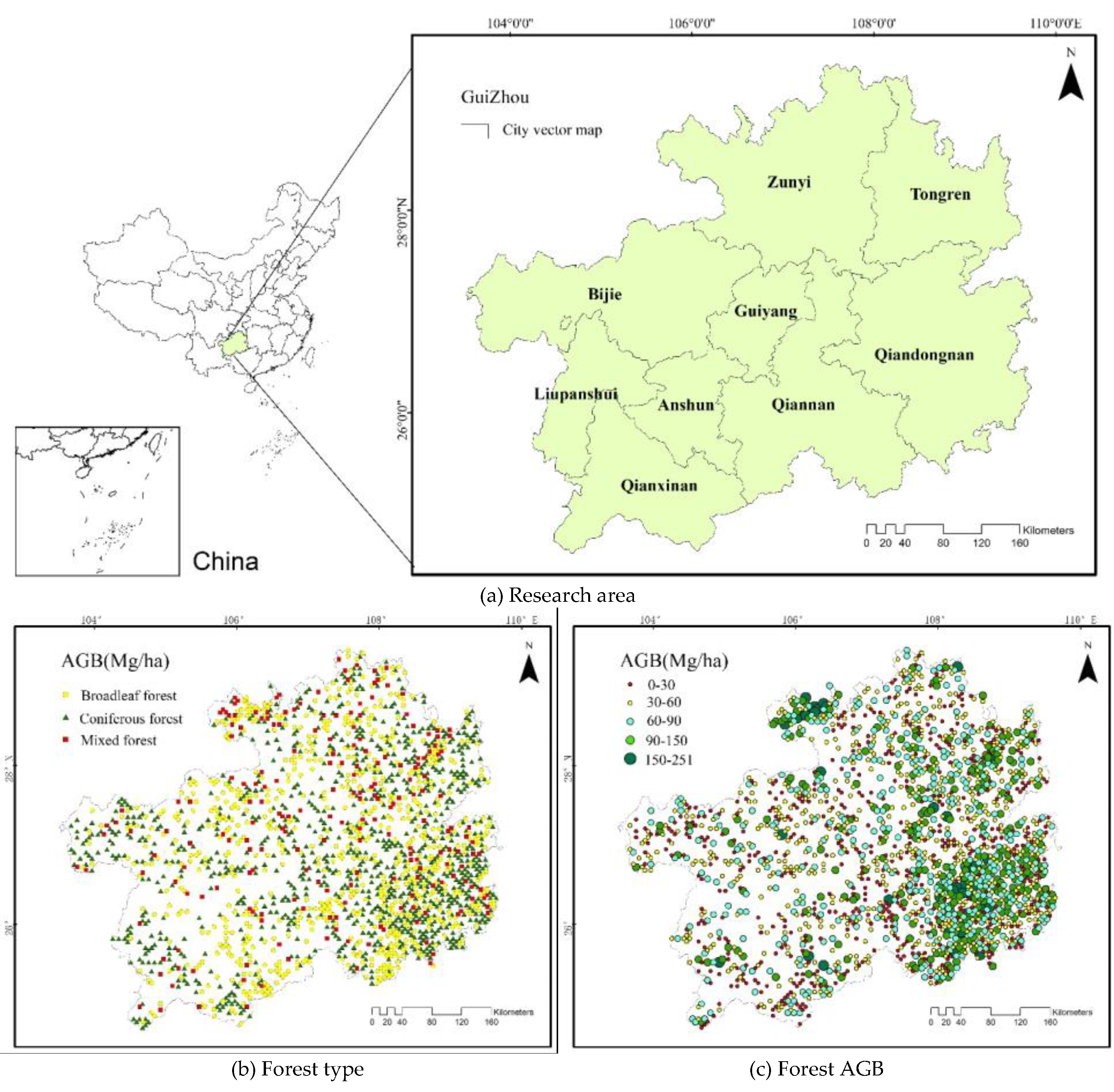
2.1. Research Area

Guizhou Province is bounded by latitude 24°37′–29°13′N, longitude 103°36′–109°35′E. It is approximately 595 km long from east to west and 509 km from north to south, with a total area of 176,200 km2 [49]. The terrain in Guizhou is high in the west and low in the east, and it tilts from the middle to the north, east, and south, with an average altitude of approximately 1100 m [50]. The landforms of the whole province are divided into four basic types: mountain, plateau, hill, and basin, with the most mountains, followed by hills, of which 92.5% are hills and mountains [51]. It was shown in Figure 1.
The plateau, monsoon, and diverse climate in Guizhou are conducive to the formation and development of various forest types [52]. The province is rich in forest vegetation types, including subtropical evergreen broadleaf forest, near tropical valley seasonal rain forest, tropical evergreen broadleaf forest, cold temperate subalpine coniferous forest, and warm coniferous forest [53]. In addition, most areas are dominated by all kinds of secondary and artificial vegetation, as well as cultivated land, shrub, plateau meadow, etc. Guizhou has widespread ecological problems such as soil erosion and rocky desertification [54,55].

2.2. Data

2.2.1. The Ground Survey Data

The ground survey data in this study came from the fixed sample plot data of NFCI in Guizhou in 2015. A kilometer grid was used to arrange the location of plots, and the square sample plots were evenly distributed. The sample plot size was 0.067 ha and the sample plot spacing was 4 × 8 km. There is a linear relationship between the forest volume in the stand and the aboveground forest biomass [56,57]. The details can be obtained from the literature [58], the formula is:
B = a × V + b
where B is forest biomass (Mg/ha), V is the forest stock (m3/ha), and a and b are coefficients. According to the dominant tree species recorded in NFCI, the sample plots were divided into three forest types: broadleaf forest (BLF), coniferous forest (CFF), and mixed forest (MXF), as shown in Appendix A. The number of sample plots of each forest type were 740, 948, and 212, respectively. The AGB statistics of different forest type sample plots are shown in Table 1.

2.2.2. Image Data

Since the forest is the growing season and luxuriant from June to September, the forest biomass reflected by the image is relatively stable; while in winter, the leaves fall off, and the forest biomass obtained by image inversion is unstable. We selected 50 image reflectance products in the summer of 2015 (June–September) (the tracking number covering Guizhou was 125–129/40–43) by Google Earth Engine, and preprocessed them, such as using NDVI maximum synthesis, splicing, and clipping. At the same time, we also finished operations such as spatial resolution resampling and coordinate system conversion. The SAR image datasets of Sentinel-1A were also from the Google Earth Engine (GEE) platform [59,60]. The size of the measured sample plots on the ground of NFCI data was 25.82 m × 25.82 m. In order to ensure a consistent resolution, the Landsat 8 OLI and Sentinel-1A image data were resampled to the same size of sample plot in this study.
In addition, the land cover classification map from the European Space Agency website (http://maps.elie.ucl.ac.be/CCI/viewer/index.php/ accessed on 20 September 2021) was obtained, as shown in Figure 2. According to the needs of this study, the CCI land cover data were resampled into a resolution consistent with the ground survey sample. The landform data comes from Karst Data Center (http://www.karstdata.cn/ accessed on 20 September 2021).
We verify the consistency between CCI land cover classification and forest types in NFCI, the results shown in Table 2. The overall accuracy is 0.894. It showed that the accuracy of CCI land classification results can be used as auxiliary data support for this study.

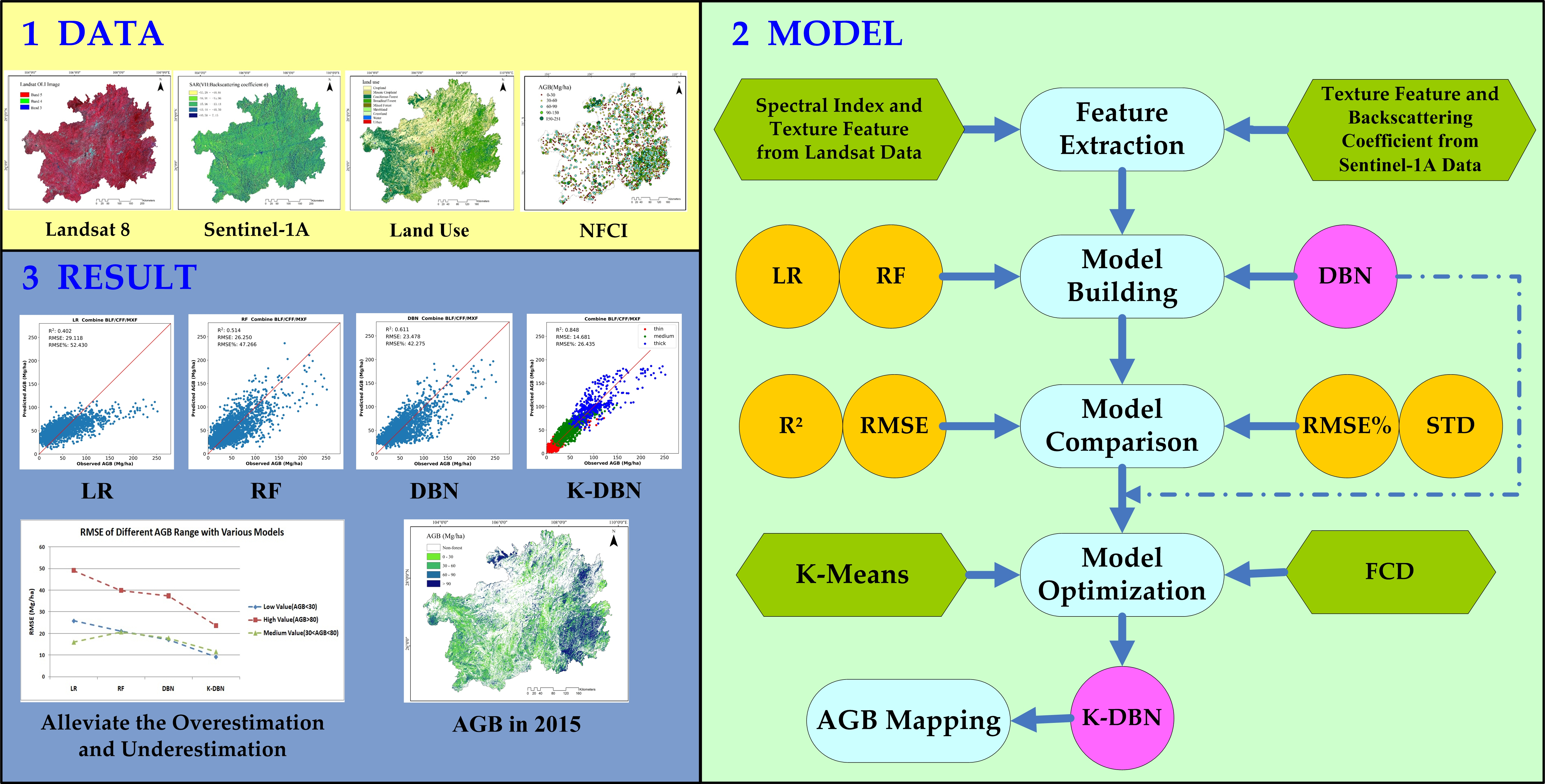
3. Technical Approach

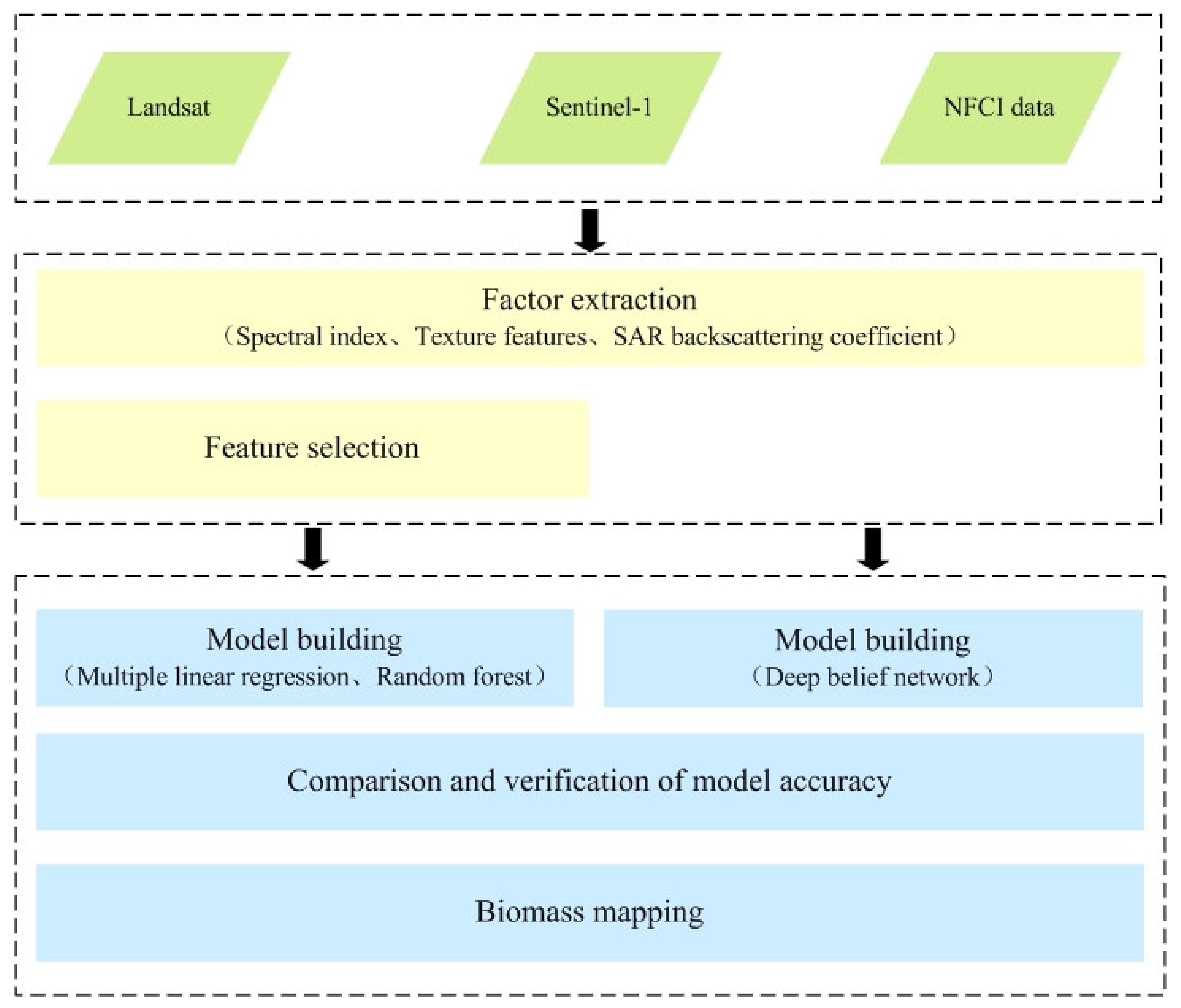
3.1. Research Workflow

The research technology workflow mainly included three layers, as shown in Figure 3. The first layer was data preparation and preprocessing, including Landsat 8 OLI, Sentinel-1A, and NFCI data. The second layer was factor extraction. We extracted the feature factors of the above-mentioned images, such as spectral data, texture features, and SAR backscattering coefficients. The third layer was the design of a DBN model, its accuracy was compared to that of LR and RF models. This study also optimized the DBN model and designed the K-DBN model, as shown in Section 4.2. Finally, spatial mapping of AGB in the whole study area was carried out.

3.2. Feature Extraction

We extracted 230 feature factors, including 30 vegetation indices, 6 Landsat 8 OLI original bands and 144 texture feature factors, and 2 SAR backscattering coefficients and 48 their texture features. They were shown in Table 3 and the details were shown in Appendix B.
The vegetation index is mainly an index reflecting the difference between vegetation reflection in visible and near-infrared bands and the soil background. It can effectively integrate relevant spectral signals, enhance vegetation information, and reduce the impact of non-vegetation information. The texture has a good interpretation of spatial structure for the estimation ability of forest AGB. In this study, the gray-level co-occurrence matrix (GLCM) method was used to extract texture features with the moving window size by 3 × 3, 5 × 5, and 7 × 7 [14].

3.3. FCD Calculation

The FCD is closely related to the growth and health of trees. Many indicators, such as crown competition factor, forest density index, and canopy density, can be used to describe forest density [22]. The FCD is the ratio of the total projected area of the tree crown on the ground under direct sunlight to the total area of this forest type. It is an important factor reflecting the forest stand structure, and it has a significant impact on forest growth, stem shape, and biomass [61]. The FCD model is mainly proposed based on the biophysical characteristics of the forest. The forest canopy density was introduced as a dummy variable to construct the K parallel DBN to improve the accuracy of biomass estimation. The K value is determined by the K-means algorithm in Section 4.2. According to the calculation formula in the literature [61], after normalization of the Landsat 8 OLI bands these indices has been calculated using the equation:
if :   N I R R e d < 0 , A V I = 0    
else :   AVI = N I R + 1 256 R e d × N I R R e d 1 / 3
SI = 256 B l u e × 256 G r e e n × 256 R e d  
BI = N I R + R e d N I R B l u e N I R + R e d + N I R + B l u e × 100 + 100
FCD = VD × SSI 1 / 2 1
where AVI is the advanced vegetation index, BI is the bare soil index, and SI is the shadow index [62]. Among them, VD is the first principal component of the principal component analysis of AVI and BI, and SSI is the linear transformation of SI. It showed that advanced vegetation index (AVI) was positively correlated with the forest AGB [62], and reacted sensitively to the vegetation quantity compared with NDVI; Therefore, the value is higher in forests and grassland with higher FCD values, and lower in forests and grassland with lower FCD values. BI is a function of the amount of bare soil, which increases with the decrease in forest density and the increase in surface exposure [62]. The FCD value was high, the SI value of forests was large, and the SI value of grassland and bare land was small.

3.4. The Linear Regression (LR) and Random Forest (RF) Model

The linear regression (LR) and random forest (RF) model, two conventional machine learning algorithms, which are often used in biomass estimation [63,64]. In the study of AGB estimation, the dependent variables are often affected by several important factors. At this time, two or more influencing factors are needed as independent variables to explain the change of dependent variables. When there is a linear relationship between multiple independent variables and dependent variables, the regression analysis is multiple linear regression. The RF model consists of several decision trees. Decision trees are fully grown, and unpruned classification and regression trees are generated by the classification and regression tree (CART) algorithm. The simple majority voting method is used to make the output of the random forest for classification and prediction. The results of all the base regressors used are averaged as the output of the random forest for the regression problem.

3.5. DBN Model Construction

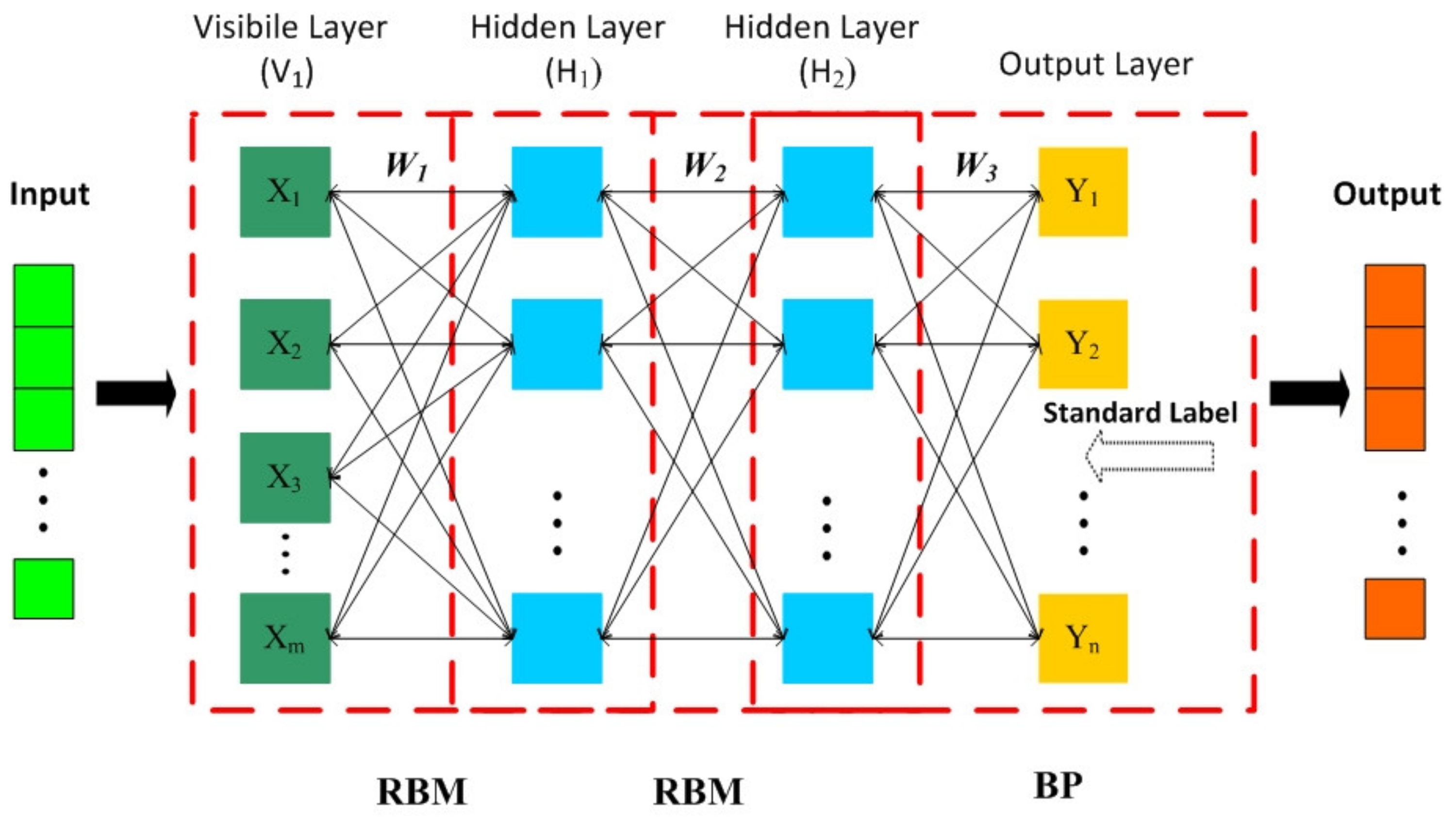
3.5.1. DBN Structure

The restricted Boltzmann machine (RBM) is a kind of neural perceptron, composed of a visible layer (the input layer) and a hidden layer, which propagates in two-way links between the two layers [65,66]. The hidden layer is the feature extraction layer we generally refer to. There is a two-way full connection between the neurons of the visible layer and the hidden layer. The back propagation (BP) is the most basic neural network [67]. Its output results adopt forward propagation, and the error adopts back propagation. The network structure of classical DBN is a deep neural network composed of a visible layer, several RBMs, and a BP, that is, several RBMs are “connected in series” to form a DBN, in which the hidden layer of the previous RBM is the explicit layer of the next RBM, and the output of the previous RBM is the input of the next RBM. In the training process, the RBM of the current layer can only be trained after fully training the RBM of the previous layer until the last layer. The layers are connected to one another, but the cells in the layer are not connected to one another. The cells in each hidden layer are trained to express advanced features. The DBN represents the most original input data with different concept granularities at each layer, that is, different levels of feature description. The structure is shown in Figure 4. Xi is characteristic factor set of samples, Yi is measured value of samples, Wi is weight coefficient.

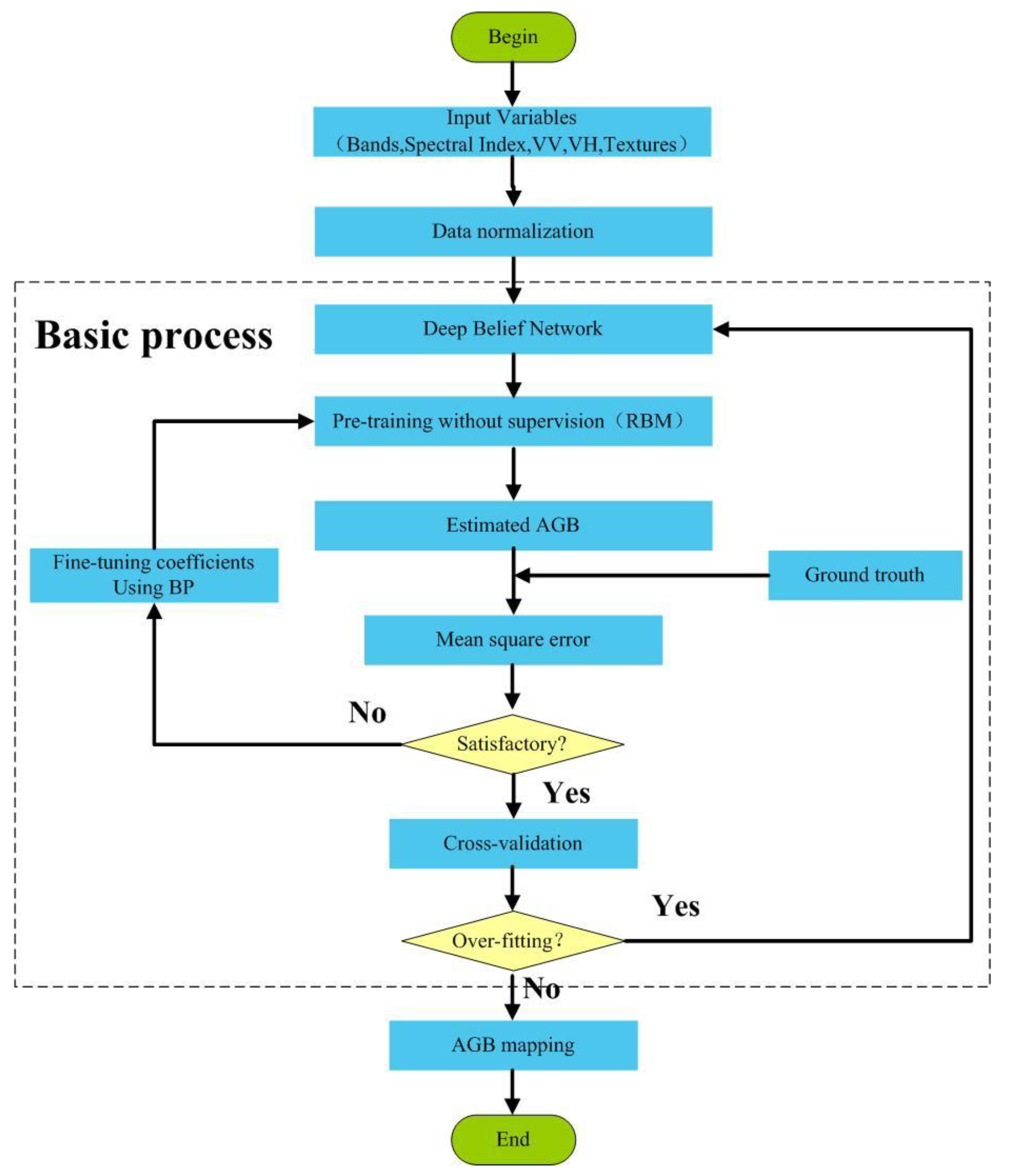
3.5.2. DBN AGB Mapping Workflow

The DBN AGB mapping workflow is shown in Figure 5. The independent variable set X , including the spectral index, texture feature, and SAR backscattering coefficients, with a total of 230 feature factors, were input into the DBN model. Then, in the model training, we designed several RBMs for unsupervised training. The output of the former RBM was used as the input of the latter RBM. At the same time, taking the marked sample as the target value, we modified it with BP feedback parameters to model the AGB estimation. Here, we compared the MSE with the ground truth and the prediction results. If the MSE did not decrease for three consecutive times, we considered that the model training was relatively stable and available, then it was further judged by 10-fold cross-validation. When the training accuracy was insufficient, it returned to the input of the DBN model, and the above steps were further repeated until the training accuracy met the conditions. Finally, spatial mapping of overall forest biomass was carried out.

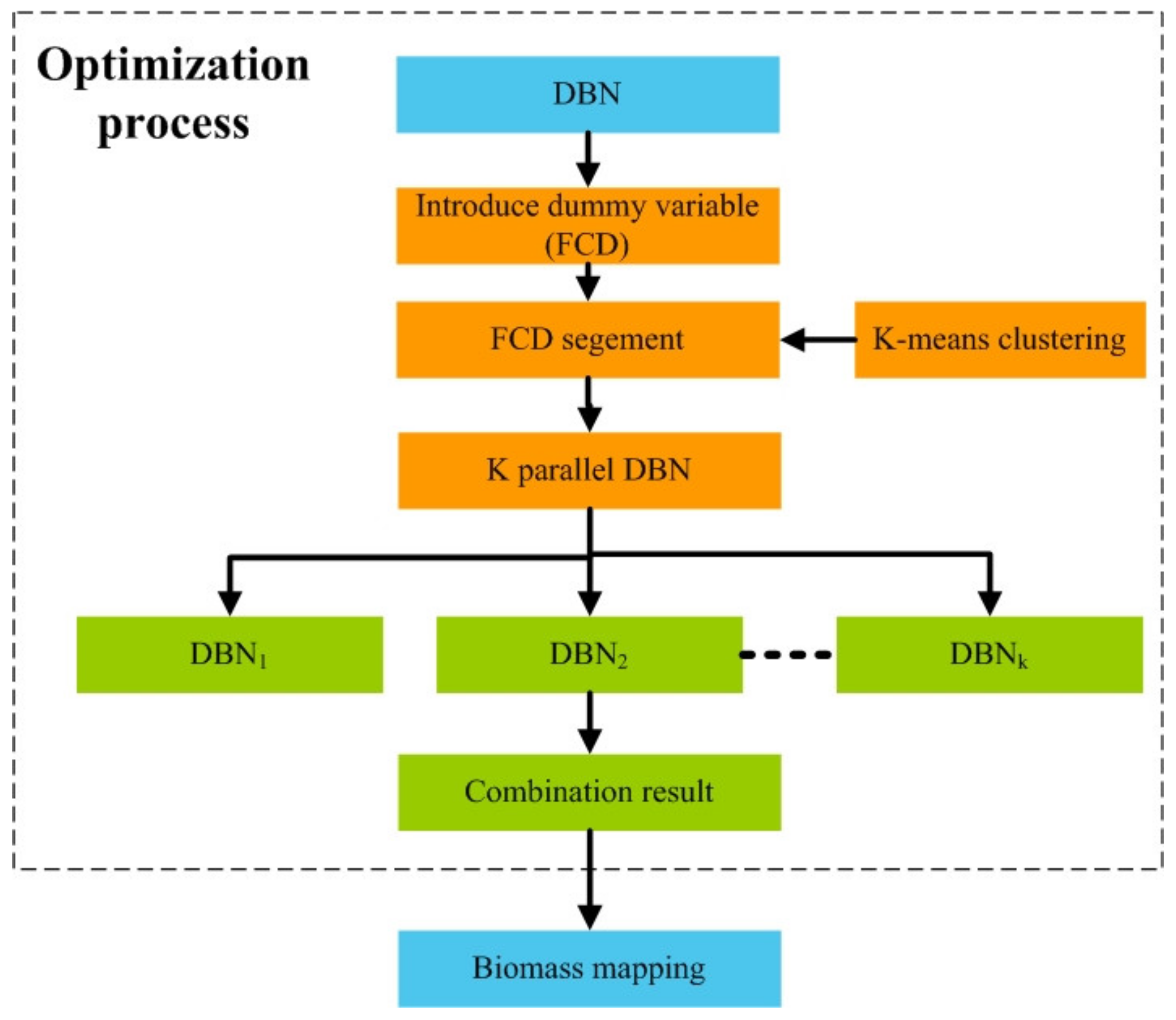
3.5.3. K-DBN Model Construction

High-value underestimation and low-value overestimation are common problems in AGB estimation models. In generally low-value overvaluation usually occurs in sparse forests with small AGB values, while high-value under estimation usually occurs in relatively dense forests with high AGB values [68]. This study considered introducing FCD to improve the DBN model to alleviate the problems of high-value underestimation and low-value overestimation. Firstly, the FCD value of each sample plot was calculated as a dummy variable. Secondly, the FCD was segmented by the K-means method, and K parallel DBN models were constructed to estimate the AGB of different FCD segments. Finally, the estimated results were combined to obtain the final result. This study defined this method as the K-DBN method, and the workflow is shown in Figure 6.

4. Results and Analysis

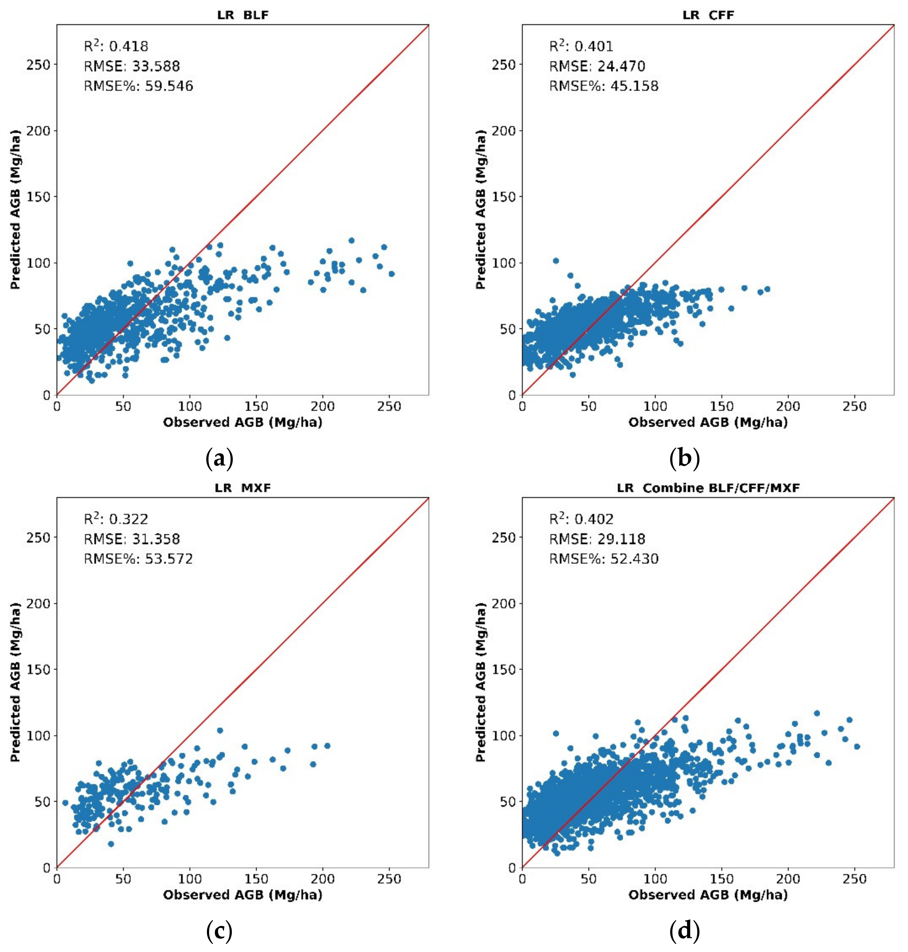
4.1. Performance of AGB Estimation Model

4.1.1. DBN Model Building

In this study, The DBN was used to construct an AGB estimation model. As a deep learning model, the DBN model inputs all feature factors, omits the step of feature factor selection, and only considers the setting of the model parameters, which directly affect the performance of the model. These parameters include the number of hidden layers, the number of knots, and the number of iterations. In this study, we analyzed and compared the DBN model parameters; the results are shown in Table 4. The parameter settings with the best performance were determined.

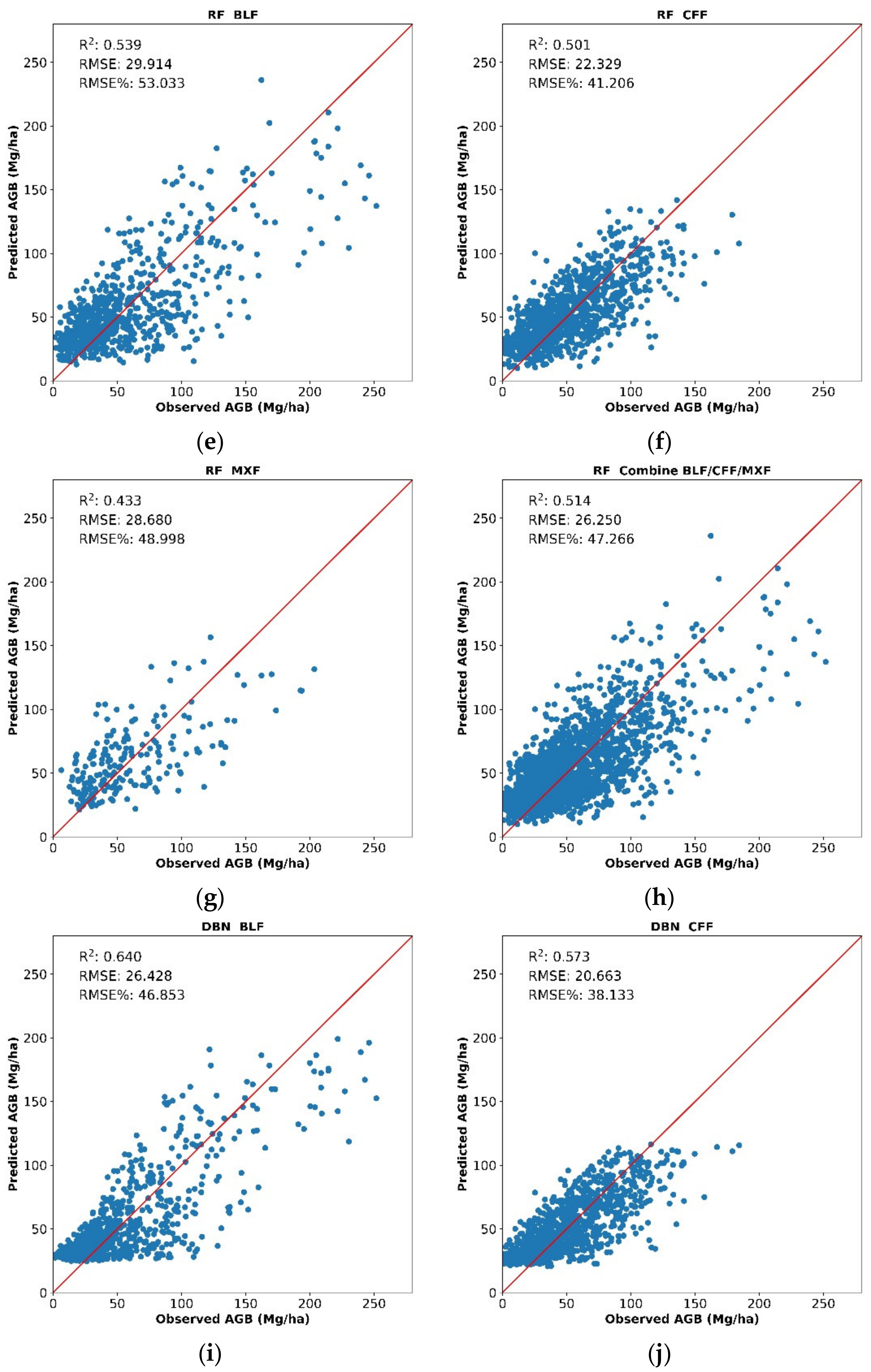
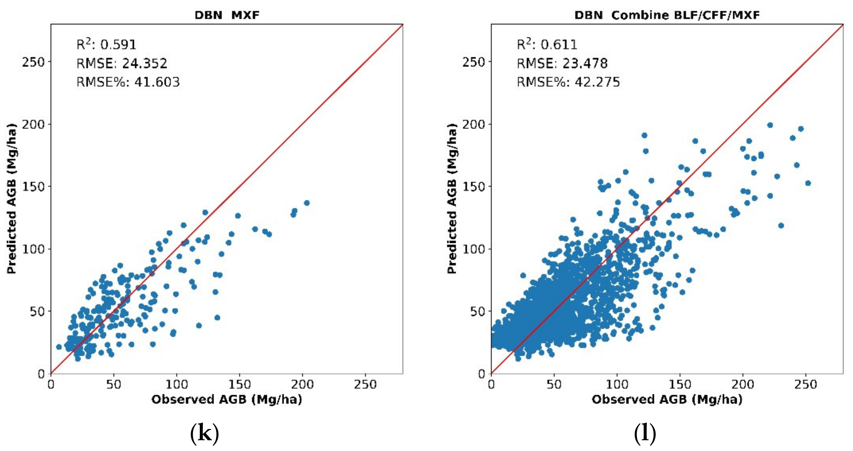
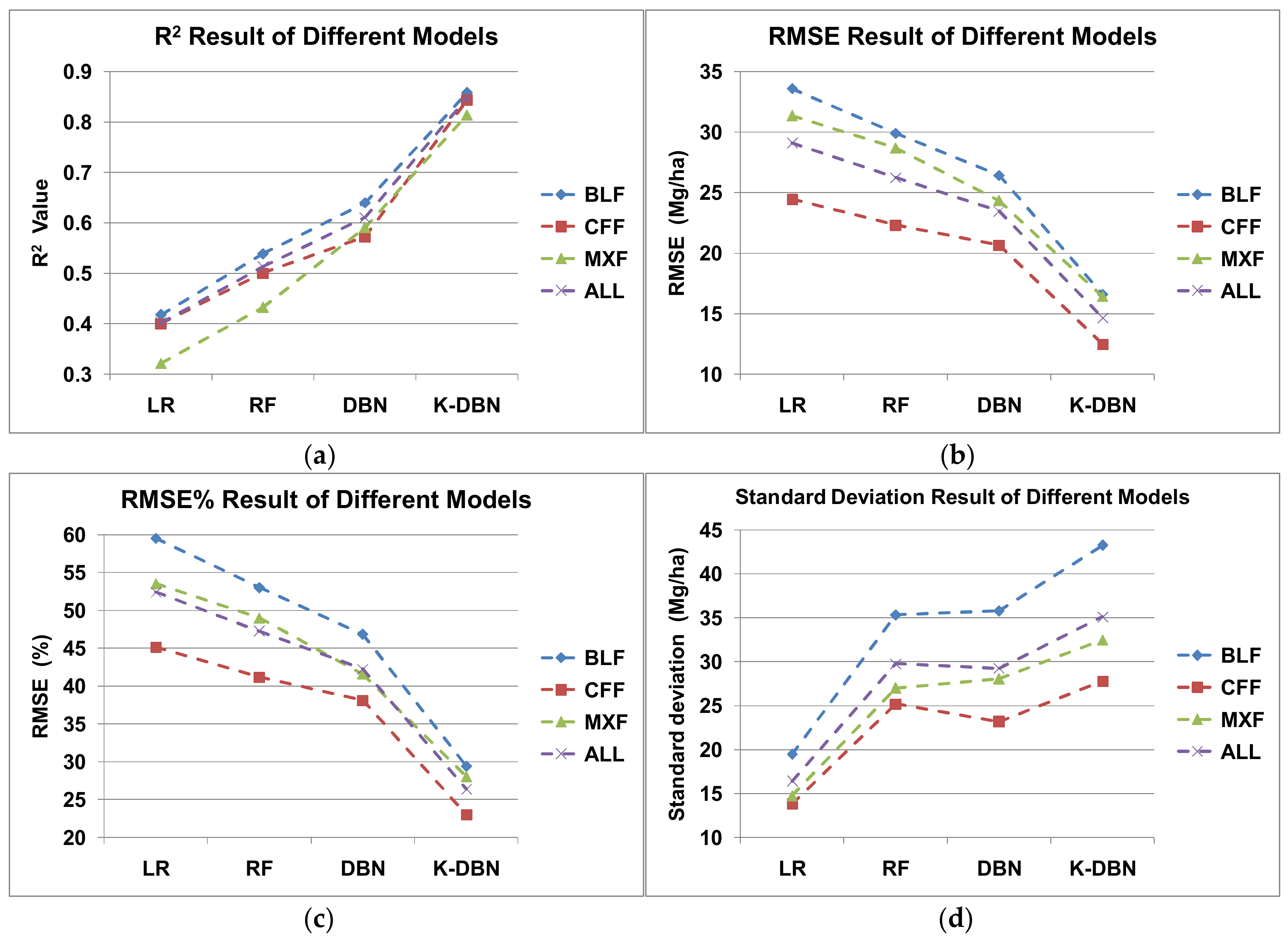
4.1.2. Model Accuracy Comparison

In this paper, The BLF, CFF, and MXF were separately set up to build the model. The AGB estimation model is constructed based on DBN and compared with LR and RF. Through 10-fold cross-validation, the prediction results of all models are shown in Figure 7.
The degree of interpretation of the LR model for the AGB estimation of various forest types was less than 45%. The overall R2 was 0.402 and the RMSE was 29.118 Mg/ha, among which, the BLF R2 and RMSE were the best, 0.418 and 33.588 Mg/ha respectively, while the CFF and MXF R2 values were 0.401 and 0.322, respectively, and the RMSE values were 24.470 and 31.358 Mg/ha, respectively.
The results of the RF model were better than those of the LR model, and the accuracy of the various forest types was higher than that of the corresponding LR model. The R2 and RMSE values were 0.514 and 26.250 Mg/ha, respectively, among which, the BLF had the highest accuracy, with R2 and RMSE values of 0.539 and 29.914 Mg/ha, followed by 0.501 and 22.329 Mg/ha for the CFF, and 0.433 and 28.680 Mg/ha for the MXF.
The DBN model had the best performance, whose determination coefficient (R2) was higher than LR and RF. The R2 increased to 0.611 and the RMSE decreased to 23.478 Mg/ha. The R2 of the BLF was the highest, reaching 0.640, with an RMSE of 26.428 Mg/ha; meanwhile, the R2 of the MXF and CFF was 0.591 and 0.573, with an RMSE of 24.352 and 20.663 Mg/ha, respectively.
In any forest type, the DBN model performs better than the RF and LR models. However, the problems of low-value overestimation occurred at the sample points of less than 30 Mg/ha, and high-value underestimate occurred at the sample points of more than 80 Mg/ha. In this study, forest canopy density was introduced as a dummy variable to improve the DBN model in order to improve the accuracy of biomass estimation.

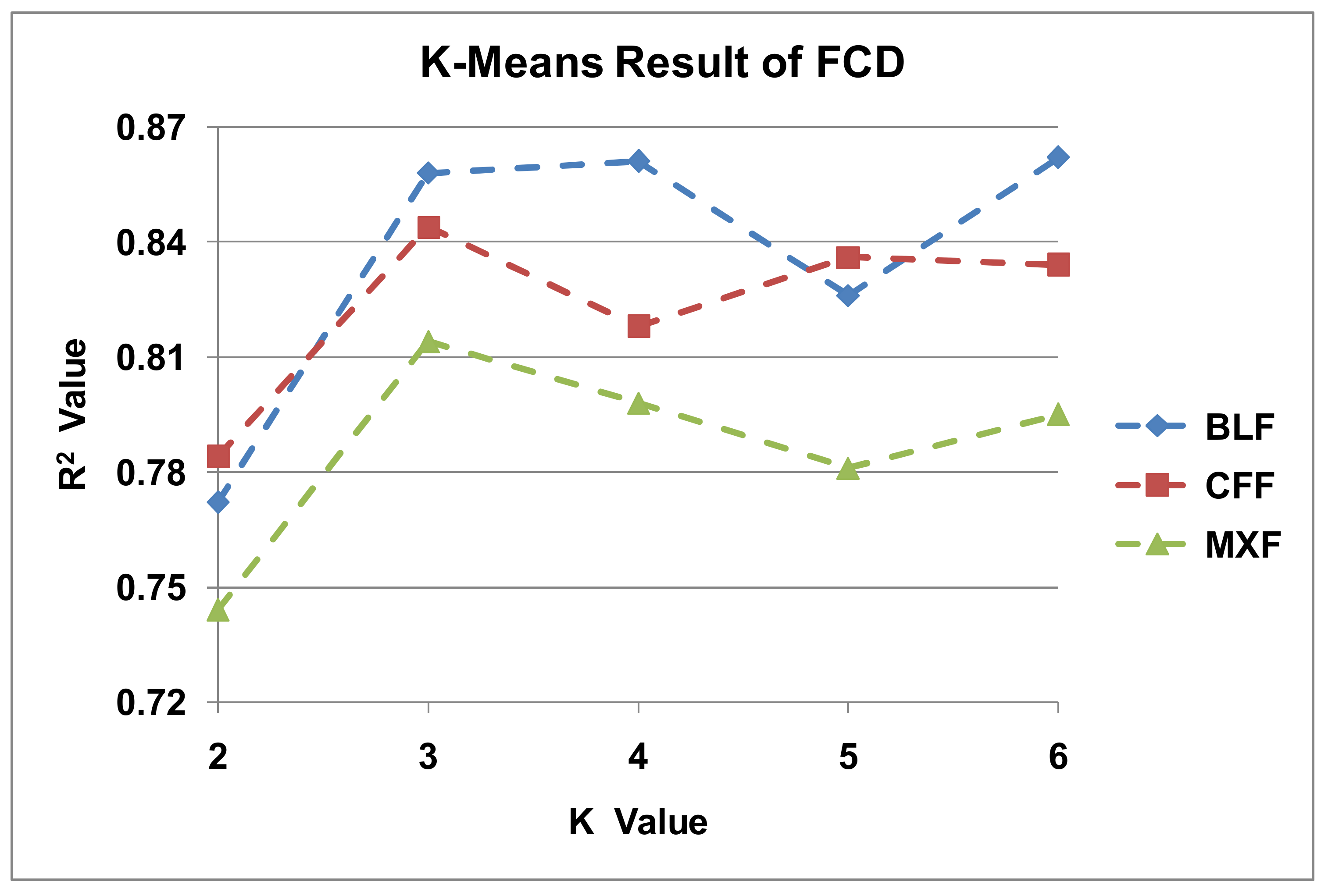
4.2. K-Value Setting of the K-DBN Model

The setting of the K-value classifies the FCD, but there is no clear classification standard of the forest canopy density in forest management. In this study, the K-means method was used to cluster FCD to determine the best K-value. In this specific study, K was taken as 2~6 to test the accuracy of the model. The results showed that for the broadleaf forest, when k is 3~6, the model R2 is basically equal. For other forests, when k is 3, the model performs best. Considering the model accuracy and the DBN algorithm execution efficiency, the number of 3 was taken in this study, that is, the samples were divided into three levels according to FCD: thin, medium, and thick. The FCD classification statistical results of the different forest types are shown in Figure 8 and Table 5. There are obvious differences in the mean AGB of the different forest types corresponding to the three grades of FCD. The mean AGB of the thin sample plot was approximately 30 Mg/ha, that of the medium sample plot was approximately 50 Mg/ha, and that of the thick sample plot was close to 100 Mg/ha. It can also be seen from Figure 9 that there is a significant positive correlation between forest AGB and FCD. Generally speaking, forest biomass with a large canopy density is larger, and forest biomass with a small canopy density is smaller. Therefore, the K-DBN model constructed after adding FCD classification can further improve the accuracy of the estimation model.

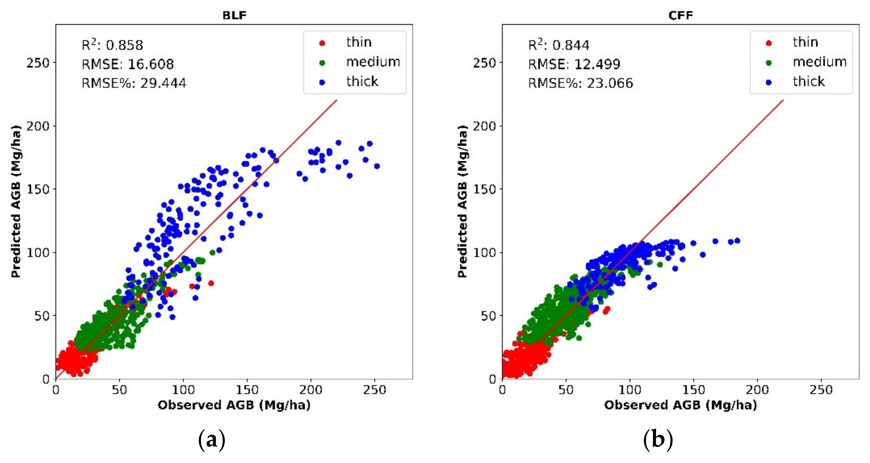
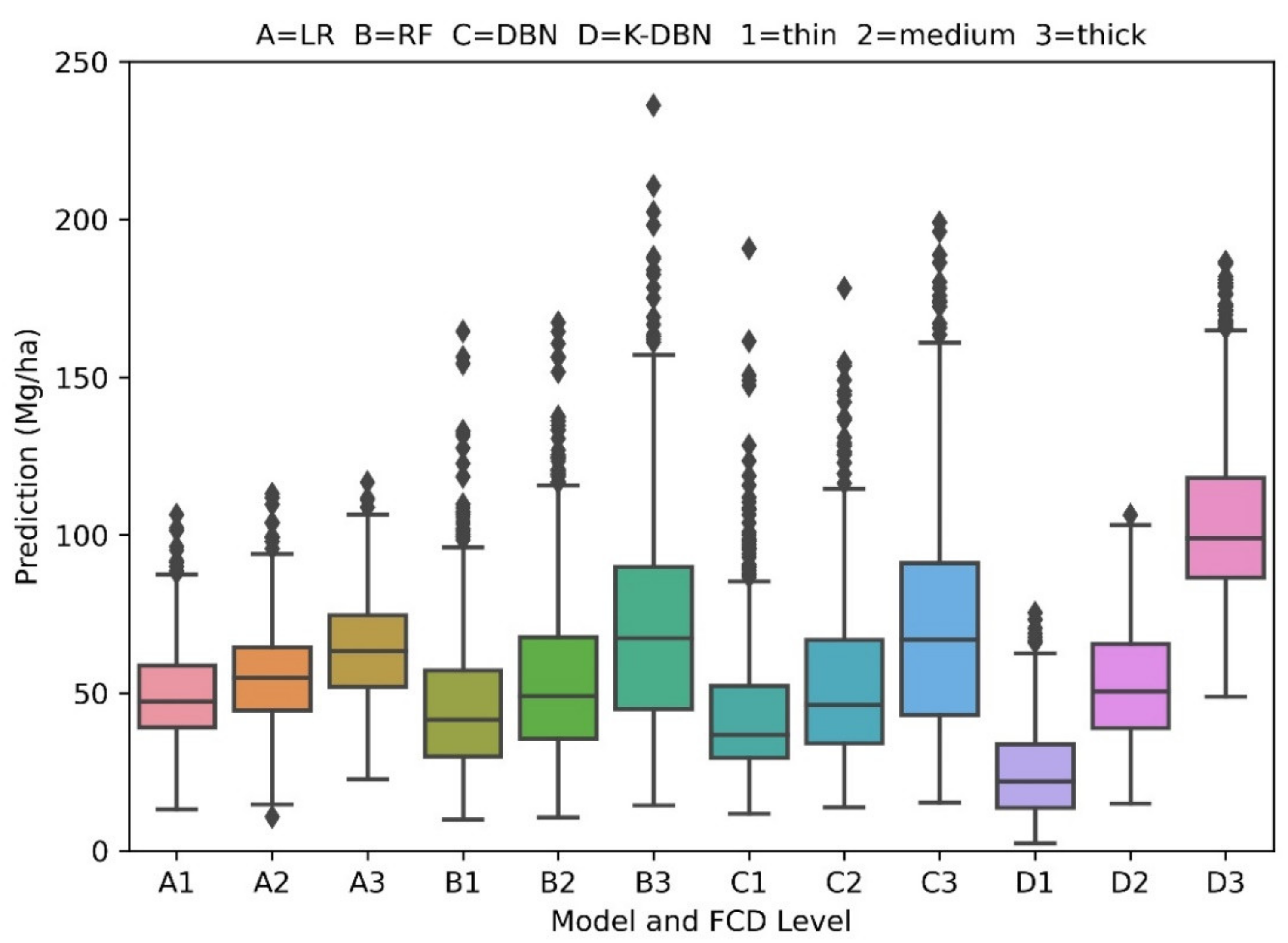
4.3. K-DBN Model Performance

According to the result of the K-means cluster analysis of FCD, the original samples were segmented first, and the K-DBN model was constructed to improve the AGB estimation accuracy. The results are shown in Figure 10. After the forest type classification, the accuracy was 0.848 and 14.681 Mg/ha, among which the highest accuracy R2 of the BLF model was 0.858, followed by the CFF with 0.844 and the MXF with 0.814, with RMSE values of 16.608, 12.499, and 16.439 Mg/ha, respectively. Compared to the traditional DBN model, the estimation accuracy of K-DBN improved, and AGB has been estimated more accurately. For the DBN model, the R2 is 0.611, RMSE is 23.478 Mg/ha. For the K-DBN model, the R2 is 0.848, RMSE is 14.681 Mg/ha, R2 increased by 0.2377 and RMSE decreased by 8.79 Mg/ha. It can be seen from Figure 10 that the K-DBN model solved the problems of high-value undervaluation and low-value overvaluation to a certain extent. From the perspective of vegetation growth, building forest biomass estimation models by forest types and canopy density can more accurately distinguish the differences in forest stand structure and coverage therefore can ensure the estimation accuracy of the classification model.
The LR, RF, DBN, and K-DBN models used in this paper were compared and ana-lyzed, as shown in Figure 11. The K-DBN had the best performance followed by DBN, RF, and LR.
It can be seen that, compared with LR, RF, and DBN, K-DBN can more accurately predict the AGB. In combination with Figure 9, the AGB distribution of the measured samples presented a small to large trend. Figure 12 showed the results of prediction at different FCD levels by the K-DBN model (D1 to D3), which of distribution was the closest to that in Figure 9. So compared with LR, RF, and DBN models, the K-DBN model can more accurately predict the AGB.
In the two biomass ranges of <30Mg/ha and >80Mg/ha, the problems of low-value overestimation and high-value underestimation are obvious [21]. In order to accurately analyze the performance of each model in low-value overestimation and high-value underestimation, the prediction RMSE of the 526 low-value sample plots (AGB < 30) and 423 high-value sample plots (AGB > 80 Mg/ha) were analyzed, and the results are shown in Figure 13.
When the AGB is 30–80 Mg/ha, there is little difference in the accuracy of various biomass estimation models. However, when the AGB is less than 30 Mg/ha or more than 80 Mg/ha, the K-DBN algorithm can improve the model accuracy effectively. In the low-value range (AGB < 30 Mg/ha), the RMSE of the K-DBN algorithm is 9.182 Mg/ha, which is 16.635 Mg/ha, 11.908 Mg/ha, and 7.966 Mg/ha lower than LR, RF, and DBN respectively. In the high-value range (AGB > 80 Mg/ha), the RMSE of the K-DBN algorithm is 23.685 Mg/ha, which is 25.370 Mg/ha, 16.141 Mg/ha, and 13.641 Mg/ha lower than LR, RF, and DBN respectively. According to the above analysis, the K-DBN algorithm significantly alleviates the problems of high-value underestimation and low-value overestimation, therefore can further improve the accuracy of AGB estimation.

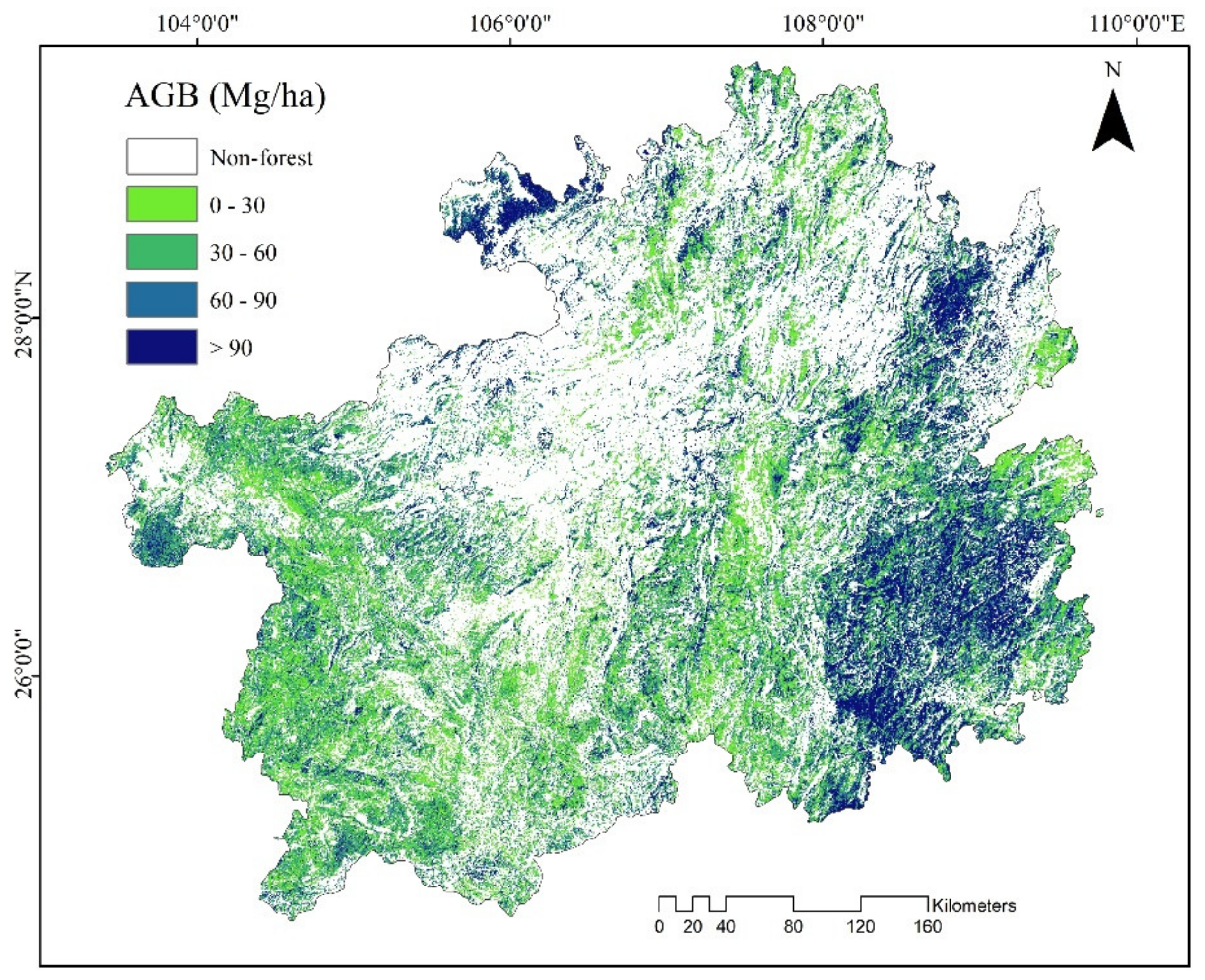
4.4. The AGB Spatial Mapping

The K-DBN model was used to map the forest AGB in the study area in 2015, as shown in Figure 14. In 2015, the predicted maximum value of forest biomass in the study area was 199.812 Mg/ha, the minimum value was 3.301 Mg/ha, the average value was 54.946 Mg/ha, and the standard deviation was 36.053 Mg/ha. Those forests with high biomass were mainly distributed in the northern and southeastern parts of Guizhou, especially in Zunyi, Tongren, and Qiandongnan. The forest biomass in Bijie, Liupanshui, and other places with serious rocky desertification was low.

5. Discussion

5.1. DBN Model Mechanism

In this study, the AGB estimation model is constructed based on a deep learning algorithm DBN, and its accuracy is significantly higher than that of the traditional LR and RF models. There are two reasons for the improvement of model accuracy. (1) DBN algorithm has a more powerful data processing ability. By fusing multi-source remote sensing data for AGB estimation, more feature factors are constructed, which inherently results in big data. Compared with traditional AGB estimation methods, such as LR and RF, feature factors need to be selected. DBN algorithm is more suitable for processing big data and can involve more feature factors in model operation. The DBN overcomes the shortcomings of the BP network which is easy to fall into local optimization and long training time due to random initialization of weight parameters. (2) The advantage of the DBN algorithm is “deep”. It reconstructs the feature factors by constructing multiple independent hidden layers (RBM), excavates the internal mechanism, better represents the complex nonlinear relationship between the feature factor set and the forest biomass, and makes the model have better interpretation ability after multiple feedback iterative modifications. Deep learning algorithms such as DBN are rarely used for forest biomass estimation, but they are indeed a good machine learning method [44]. The deep learning algorithm shows its advantages over the traditional algorithm. It is consistent with literature research. Wang et al. [69] used LR, GRNN (radial basis function network), BPNN (back propagation neural network), and DBN models to estimate the snow thickness of Alaska, and R2 is 0.48, 0.72, 0.80, and 0.85 respectively, and The DBN model performed the best. Bai et al. [70] used the DBN model to carry out analog detection of gas turbines, and R2 was 0.11 higher than that of the LR model. Duan et al. [71] estimated rice biomass using the DBN model, and compared it with the LR model, R2 increased by 0.12. However, it should be noted that we only apply one type of deep learning model to model AGB. Other deep learning models (such as CNN and RNN) further consider the spatial structure relationship between feature factors, and whether they can better estimate AGB is worthy of further research [72]. Deep learning is a promising modeling method for AGB estimation, but there is still room for improvement.

5.2. K-DBN Alleviate the Overestimation and Underestimation

The phenomena of low-value overestimation and high-value underestimate are inevitable problems in AGB estimation using remote sensing data. This is because there is image pixel saturation, especially in the field of optical remote sensing. So such problems were also inevitable. When the forest density is high to a certain extent and the forest has a complex structure [73], the remote sensing image is no longer sensitive to the change of the forest AGB, and the image information no longer changes with the increase of the forest AGB, resulting in the saturation of the image information and the underestimation of the high value of the forest AGB. In this paper, the traditional DBN algorithm is improved and preceded by a clustering process, that is, the sample points are merged into different clusters so that the biomass in different value ranges of high, medium, and low, has a boundary [74], which avoids the high bias of low values and the low bias of high values. The FCD has a strong correlation with forest biomass, especially in the high-value range and low-value range, so it is a good clustering factor. In this paper, the K-DBN model is constructed by adding FCD, and the accuracy of the model is greatly improved. Li et al. [21] proved that canopy density is a good segmentation factor, which can improve the estimation accuracy of the model. It is consistent with this paper. This effective method of K-mean clustering before regression can improve the accuracy of the model. It is proved by the literature research [75,76]. This study solved the problems of low-value overestimation and high-value underestimation in the low-value range of 10–30 Mg/ha and the high-value range of 80–150 Mg/ha, but there were still problems in biomass less than 10 Mg/ha and more than 150 Mg/ha. In future research, we will try to find a new method to express more differences in the forest vertical mechanism. We can consider hyperspectral images and LiDAR data to obtain forest DBH and tree height parameters, combine both features of the vertical and horizontal structure, or integrate environmental and climatic factors to improve the estimation accuracy of forest biomass.

6. Conclusions

In this study, Landsat 8 OLI and Sentinel-1A image datasets were used to estimate the AGB in Guizhou, China, a typical karst area, using the deep learning algorithm (DBN), which improved the estimation accuracy for forest AGB and provided data support for the study of forest productivity, carbon sink calculation, and rocky desertification control. The NFCI data were used as ground samples, vegetation index, and texture feature factors were extracted. The determination coefficient R2 of DBN is 0.602, which is 0.208, 0.101 higher than that of the traditional linear model and RF model. In order to solve the common problems of low-value overestimation and high-value underestimate in the AGB estimation model, this study introduced FCD and used K-means to cluster the FCD into three grades, namely, thin, medium, and thick, to design a K-DBN model. The results showed that the estimation accuracy of the forest AGB of the K-DBN model was further improved, and R2 reached 0.848. The K-DBN model was used to map the AGB in the study area in 2015, which can provide data support for the study of ecological environment, carbon sink calculation, and rocky desertification control.

Author Contributions

Conceptualization: C.Q., H.Q. and M.L.; data curation: C.Q., H.Q. and F.W.; formal analysis: C.Q. and M.L.; funding acquisition: M.L.; investigation: C.Q. and M.L.; methodology: C.Q. and M.L.; project administration: C.Q. and M.L.; resources: M.L.; software: C.Q. and H.Q.; supervision: M.L.; validation: C.Q., M.L.; visualization: C.Q., H.Q. and F.W.; writing original draft: C.Q.; writing review and editing: C.Q. and H.Q. All authors have read and agreed to the published version of the manuscript.

Funding

This research was funded by the National Natural Science Foundation of China, grant number 31770679, Jiangsu Modern Agricultural Industrial Technology System Project, grant number JATS-2020-344 and JATS-2021-383, and supported by the Overseas Research Program of Jiangsu University.

Data Availability Statement

Not applicable.

Conflicts of Interest

The authors declare no conflict of interest. The founding sponsors had no role in the design of the study; in the collection, analyses, or interpretation of data; in the writing of the manuscript; nor in the decision to publish the results.

Appendix A

Table A1. The classification basis of forest types.
Forest TypeDivision CriteriaDominant Tree SPECIES group
BLFBroad-leaved pure forest (single broad-leaved tree stock ≥65%) and broad-leaved mixed forest (total broad-leaved tree stock ≥65%)Birch, sweetgum, eucalyptus, Robinia pseudoacacia, locust, alamo, Paulownia, camphor tree, Camphora officinarum, other broad-leaved trees
CCFConiferous pure forest (single coniferous tree stock ≥65%) and coniferous mixed forest (total coniferous tree stock ≥65%)Pinus armandi, cedarwood, Keteleeria fortunei, Pinus yunnanensis, Cryptomeria fortunei, masson pine, metasequoia, and other pine trees
MXFConiferous and broad-leaved mixed forest (the total volume of coniferous or broad-leaved trees accounts for 35~65%)Coniferous and broad-leaved trees

Appendix B

Table A2. List of variables.
Variable TypeVariation NumberVariable NameSpectral Bands and Vegetation IndicesFormula
Reflectance6BandsRed, Green, Blue, NIR, SWIR1, and SWIR2
Vegetation Index30ARVIAtmospherically Resistant Vegetation Index N I R 1.7 × R e d + 0.7 × B l u e / N I R + 1.7 × R e d 0.7 × B l u e Huete, et al. [77]
CVIChlorophyll II Vegetation Index N I R × Red / G r e e n 2 Vincini, et al. [78]
DVIDifference Vegetation Index NIR Red Tucker, et al. [79]
EVIEnhanced Vegetation Index 2.5 N I R R e d / I R + 6 × R e d 7.5 × B l u e + 1 Huete, et al. [80]
GARIGreen Atmospherically Resistant Index N I R G r e e n γ B l u e R e d N I R + G r e e n γ B l u e R e d Gitrlson, et al. [81]
GDVIGreen Difference Vegetation Index   NIR 2 Red 2   /   NIR 2 + Red 2 Wu, et al. [82]
GNDVIGreen Normalized Difference Vegetation Index   NIR Green / NIR + Green Gitelson, et al. [83]
GRVIGreen Ration Vegetation Index N I R / G r e e n 1 -1Sripada, et al. [84]
GSAVIGreen Soil Adjusted Vegetation Index 1.5 × N I R G r e e n / N I R + G r e e n + 0.5 Sripada, et al. [85]
IPVIInfrared Percentage Vegetation Index N I R /(NIR+Red)Crippen, et al. [86]
LAILeaf Area Index 3.618 × E V I 0.118 Boegh, et al. [87]
MSRIModified Simple Ration Index N I R / R e d 1 / N I R / R e d + 1 Chen, et al. [88]
MSAVI2Modified Soil Adjusted Vegetation Index 2 2 × N I R + 1 2 × N I R + 1 2 8 × N I R R e d / 2 Qi, et al. [89]
NDVINormalized Difference Vegetation Index   NIR Red   /   NIR + Red   Huete, et al. [80]
NLINon-Linear Vegetation Index   NIR 2 Red   / NIR 2 + R e d Geol, et al. [90]
OSAVIOptimized l Adjusted Vegetation Index N I R R e d / N I R + R e d + 0.16 Rondeaux, et al. [91]
RDVIRenormalized Difference Vegetation Index N I R R e d / N I R + R e d Roujean, et al. [92]
RVIRatio Vegetation Index R e d / N I R Towers, et al. [93]
SAVISoil Adjusted Vegetation Index 1.5 × N I R R e d / N I R + R E D + 0.5 Jordan, et al. [94], Huete, et al. [95]
SLAVISpecific Leaf Area Vegetation Index N I R / R e d + S W I R Huete, et al. [95]
SRSimple Ratio Index SR N I R / R e d Birth, et al. [96], Colombo, et al. [97]
TCATasseled Cap Angle arctan   T C G / T C B Powell, et al. [98]
TCDTasseled Cap Distance TCB × TCB TCG × TCG 2 Duane, et al. [99]
TCDITasseled Cap Disturbance Index TCB TCG + TCW Healey, et al. [100]
TGITriangular Greenness Index R e d B l u e R e d G r e e n R e d G r e e n R e d B l u e / 2 Hunt, et al. [101,102]
VARIVisible Atmospherically Resistant Index G r e e n R e d / G r e e n + R e d B l u e Gitelson, et al. [103]
TCWTasseled Cap Wetness0.1446TM1 + 0.1761TM2 + 0.3322TM3 + 0.3396TM4 − 0.6210TM5 − 0.4186TM7Price, et al. [104]
TCGTasseled Cap Greenness0.2728TM1 − 0.2174TM2 − 0.5508TM3 + 0.7221TM4 + 0.0733TM5 − 0.1648TM7Rogan, et al. [105]
TCBTasseled Cap Brightness0.2909TM1 + 0.2493TM2 + 0.4806TM3 + 0.5568TM4 + 0.4438TM5 + 0.1706TM7Luneetta, et al. [106], Price, et al. [104]
TDVITransformed Difference Vegetation Index 1.5 × N I R R e d / N I R 2 + R e d + 0.5 Bannari, et al. [107]
Texture feature144GLCMGray-level co-occurrence matrix (CON, DIS, AVG, IDM, ENT, ASM, VAR, and COR)(Contrast, dissimilarity, sum average, inverse difference moment, entropy, angle second moment, variance, and correlation) (window sizes of 3 × 3, 5 × 5, and 7 × 7 pixels)
Sentinel-1A2BandsVV and VH
48GLCMGray-level co-occurrence matrix (CON, DIS, AVG, IDM, ENT, ASM, VAR, and COR)(Contrast, dissimilarity, sum average, inverse difference moment, entropy, angle second moment, variance, and correlation)

References

  1. Fang, J.; Chen, A.; Peng, C.; Zhao, S.; Ci, L. Changes in Forest Biomass Carbon Storage in China Between 1949 and 1998. Science 2001, 292, 2320–2322. [Google Scholar] [CrossRef] [PubMed]
  2. Tang, X.G.; Li, D.W.; Wang, Z.M. Research progress of Forest Aboveground Biomass Estimation by remote sensing. Chin. J. Ecol. 2012, 31, 1311–1318. [Google Scholar]
  3. Zhang, Z.; Tian, X.; Chen, E.X. Review on estimation methods of Forest Aboveground Biomass. J. Beijing For. Univ. 2011, 33, 144–150. [Google Scholar]
  4. Kauppi, P.E.; Mielikainen, K.; Kuusela, K. Biomass and Carbon Budget of European Forests, 1971 to 1990. Science 1992, 256, 70–74. [Google Scholar] [CrossRef] [Green Version]
  5. Brown, S. Measuring carbon in forests: Current status and future challenges. Environ. Pollut. 2002, 116, 363–372. [Google Scholar] [CrossRef]
  6. Li, D.R.; Wang, C.W.; Hu, Y.M. Research progress of forest biomass estimation by remote sensing technology. Geomat. Inf. Sci. Wuhan Univ. 2012, 37, 631–635. [Google Scholar]
  7. Brown, S.; Sathaye, J.; Cannell, M. Mitigation of Carbon Emissions to the Atmosphere by Forest Management. Commonw. For. Rev. 1996, 75, 80–91. [Google Scholar]
  8. Xu, X.L.; Cao, M.K.; Li, K.R. Temporal and spatial dynamics of vegetation carbon storage in forest ecosystem in China. Prog. Geogr. 2007, 26, 1–10. [Google Scholar]
  9. Lu, D.; Batistella, M.; Moran, E. Satellite Estimation of Aboveground Biomass and Impacts of Forest Stand Structure. Photogramm. Eng. Remote Sens. 2005, 71, 967–974. [Google Scholar] [CrossRef] [Green Version]
  10. He, Q.; Chen, E.; An, R.; Li, Y. Above-Ground Biomass and Biomass Components Estimation Using LiDAR Data in a Coniferous Forest. Forests 2013, 4, 984–1002. [Google Scholar] [CrossRef] [Green Version]
  11. Allouis, T.; Durrieu, S.; Vega, C.; Couteron, P. Stem volume and above-ground biomass estimation of individual pine trees from LiDAR Data: Contribution of full-waveform signals. IEEE J. Sel. Top. Appl. Earth Obs. Remote Sens. 2013, 6, 924–934. [Google Scholar] [CrossRef]
  12. Zhao, J.; He, Y.J.; Li, Z.K. Sustainable forest management strategy in China under the background of low carbon economy. World For. Res. 2012, 25, 1–5. [Google Scholar]
  13. Sarker, M.L.; Nichol, J.; Iz, H.B. Forest biomass estimation using texture measurements of high-resolution dual-polarization C-Band SAR Data J. IEEE Trans. Geosci. Remote Sens. 2013, 51, 3371–3384. [Google Scholar] [CrossRef]
  14. Li, Y.; Li, C.; Li, M.; Liu, Z. Influence of Variable Selection and Forest Type on Forest Aboveground Biomass Estimation Using Machine Learning Algorithms. Forests 2019, 10, 1073. [Google Scholar] [CrossRef] [Green Version]
  15. Houghton, R.A.; Hall, F.; Goetz, S.J. Importance of Biomass in the Global Carbon Cycle. J. Geophys. Res. Bio Geosci. 2009, 114, 935. [Google Scholar] [CrossRef]
  16. Liu, Q.; Yang, L.; Liu, Q.H.; Li, J. Review on remote sensing retrieval methods of Forest Aboveground Biomass. J. Remote. Sens. 2015, 19, 62–74. [Google Scholar]
  17. Crosby, M.K.; Matney, T.G.; Schultz, E.B.; Evans, D.L.; Grebner, D.L.; Londo, H.A.; Rodgers, J.C.; Collins, C.A. Consequences of Landsat Image Strata Classification Errors on Bias and Variance of Inventory Estimates: A Forest Inventory Case Study. IEEE J. Sel. Top. Appl. Earth Obs. Remote Sens. 2017, 10, 243–251. [Google Scholar] [CrossRef]
  18. Yang, W.Z.; Zhao, P.X.; Xue, D.Q. Study on forest biomass estimation model of Nanbei mountain in Xining City Based on landsat-8 image. J. Northwest For. Univ. 2016, 31, 33–37. [Google Scholar] [CrossRef]
  19. Xu, T.; Cao, L.; Shen, G.H. Optimal extraction of characteristic variables and forest biomass inversion based on Landsat 8 OLI. Remote. Sens. Technol. Appl. 2015, 30, 226–234. [Google Scholar]
  20. Lu, C.; Zhang, J.L.; Wang, A.Y.; Jiang, S.C.; Huang, C.X.; Luo, Y.J. Biomass estimation and reconstruction of Pinus Takayama in Shangri La based on Landsat TM. For. Inventory Plan. 2016, 41, 1–7. [Google Scholar]
  21. Li, C.; Li, Y.; Li, M. Improving Forest Aboveground Biomass (AGB) Estimation by Incorporating Crown Density and Using Landsat 8 OLI Images of a Subtropical Forest in Western Hunan in Central China. Forests 2019, 10, 104. [Google Scholar] [CrossRef] [Green Version]
  22. Joshi, C.; De Leeuw, J.; Skidmore, A.K.; van Duren, I.C.; van Oosten, H. Remotely sensed estimation of forest canopy density: A comparison of the performance of four methods. Int. J. Appl. Earth Obs. Geoinf. 2006, 8, 84–95. [Google Scholar] [CrossRef]
  23. Ou, G.; Li, C.; Lv, Y.; Wei, A.; Xiong, H.; Xu, H.; Wang, G. Improving aboveground biomass estimation of pinus densata forests in yunnan using landsat 8 imagery by incorporating age dummy variable and method comparison. Remote Sens. 2019, 11, 738. [Google Scholar] [CrossRef] [Green Version]
  24. Tigges, J.; Churkina, G.; Lakes, T. Modeling above-ground carbon storage: A remote sensing approach to derive individual tree species information in urban settings. Urban Ecosyst. 2016, 20, 97–111. [Google Scholar] [CrossRef]
  25. Mermoz, S.; Réjou-Méchain, M.; Villard, L.; Le Toan, T.; Rossi, V.; Gourlet-Fleury, S. Decrease of L-band SAR backscatter with biomass of dense forests. Remote. Sens. Environ. 2015, 159, 307–317. [Google Scholar] [CrossRef]
  26. Kumar, S.; Khati, U.G.; Chandola, S.; Agrawal, S.; Kushwaha, S.P. Polarimetric SAR Interferometry based modeling for tree height and aboveground biomass retrieval in a tropical deciduous forest. Adv. Space Res. 2017, 60, 571–586. [Google Scholar] [CrossRef]
  27. Santi, E.; Paloscia, S.; Pettinato, S.; Fontanelli, G.; Mura, M.; Zolli, C.; Maselli, F.; Chiesi, M.; Bottai, L.; Chirici, G. The potential of multifrequency SAR images for estimating forest biomass in Mediterranean areas. Remote Sens. Environ. 2017, 200, 63–73. [Google Scholar] [CrossRef]
  28. Benson, M.L.; Pierce, L.; Bergen, K.; Sarabandi, K. Model-Based Estimation of Forest Canopy Height and Biomass in the Canadian Boreal Forest Using Radar, LiDAR, and Optical Remote Sensing. IEEE Trans. Geosci. Remote Sens. 2010, 59, 4635–4653. [Google Scholar] [CrossRef]
  29. Zhu, Y.; Feng, Z.; Lu, J.; Liu, J. Estimation of Forest Biomass in Beijing (China) Using Multisource Remote Sensing and Forest Inventory Data. Forests 2020, 11, 163. [Google Scholar] [CrossRef] [Green Version]
  30. Chen, L.; Wang, Y.; Ren, C.; Zhang, B.; Wang, Z. Optimal combination of predictors and algorithms for forest above-ground biomass mapping from sentinel and SRTM data. Remote Sens. 2019, 11, 414. [Google Scholar] [CrossRef] [Green Version]
  31. Laurin, G.V.; Pirotti, F.; Callegari, M.; Chen, Q.; Cuozzo, G.; Lingua, E.; Notarnicola, C.; Papale, D. Potential of ALOS2 and NDVI to Estimate Forest Above-Ground Biomass, and Comparison with Lidar-Derived Estimates. Remote Sens. 2016, 9, 18. [Google Scholar] [CrossRef] [Green Version]
  32. Chen, L.; Ren, C.; Zhang, B.; Wang, Z.; Xi, Y. Estimation of forest above-ground biomass by geographically weighted regression and machine learning with sentinel imagery. Forests 2018, 9, 582. [Google Scholar] [CrossRef] [Green Version]
  33. Li, Y.; Li, M.; Li, C.; Liu, Z. Forest aboveground biomass estimation using Landsat 8 and Sentinel-1A data with machine learning algorithms. Sci. Rep. 2020, 10, 9952. [Google Scholar] [CrossRef] [PubMed]
  34. Minh, D.H.T.; Ndikumana, E.; Vieilledent, G.; McKey, D.; Baghdadi, N. Potential value of combining ALOS PALSAR and Landsat-derived tree cover data for forest biomass retrieval in Madagascar. Remote Sens. Environ. 2018, 213, 206–214. [Google Scholar] [CrossRef]
  35. Li, X.; Ye, J.A. Estimation of vegetation biomass in mangrove wetland by radar remote sensing. J. Remote. Sens. 2006, 10, 387–396. [Google Scholar]
  36. Guo, Q.X.; Zhang, F. Estimation of forest biomass based on Remote Sensing Information. J. Northeast. For. Univ. 2003, 31, 13–16. [Google Scholar]
  37. Wu, Y.; Zhang, H.Y.; Lu, T.F.; Xu, H.; Ou, G.L. Establishment of remote sensing estimation model of biomass on alpine and subalpine coniferous forest land in Northwest Yunnan and determination of light saturation point based on Landsat 8 OLI. J. Yunnan Univ. 2021, 43, 818–830. [Google Scholar]
  38. Zhao, P.; Lu, D.; Wang, G.; Wu, C.; Huang, Y.; Yu, S. Examining Spectral Reflectance Saturation in Landsat Imagery and Corresponding Solutions to Improve Forest Aboveground Biomass Estimation. Remote Sens. 2016, 8, 469. [Google Scholar] [CrossRef] [Green Version]
  39. Li, C.; Li, M.; Li, Y. Improving estimation of forest aboveground biomass using Landsat 8 imagery by incorporating forest crown density as a dummy variable. Can. J. For. Res. 2020, 50, 390–398. [Google Scholar] [CrossRef]
  40. Wang, L.; Liu, J.; Xu, S.; Dong, J.; Yang, Y. Forest Above Ground Biomass Estimation from Remotely Sensed Imagery in the Mount Tai Area Using the RBF ANN Algorithm. Intell. Autom. Soft Comput. 2018, 24, 391–398. [Google Scholar] [CrossRef]
  41. Ghosh, S.M.; Behera, M. Aboveground biomass estimation using multi-sensor data synergy and machine learning algorithms in a dense tropical forest. Appl. Geogr. 2018, 96, 29–40. [Google Scholar] [CrossRef]
  42. Dang, A.; Nandy, S.; Srinet, R.; Luong, N.V.; Ghosh, S.; Kumar, A.S. Forest aboveground biomass estimation using machine learning regression algorithm in Yok Don National Park, Vietnam. Ecol. Inform. 2019, 50, 24–32. [Google Scholar] [CrossRef]
  43. Jiang, Z.C.; Ma, Y.; Jiang, T.; Chen, C. Research on Hyperspectral Remote Sensing Extraction of Red Tide Based on depth confidence network (DBN). Ocean Technol. 2019, 38, 1–7. [Google Scholar]
  44. Liu, L.C.; Xiong, K.N.; Luo, Y. Advances in Evaluation of Sustainable Development Capability in Karst Region. Guizhou Agric. Sci. 2012, 40, 67–72. [Google Scholar]
  45. Pan, G.Y.; Cai, W.; Qiao, J.F. Depth determination method of DBN network. Control Decis. 2015, 30, 256–260. [Google Scholar]
  46. Ma, S.B.; Yang, G.B.; An, Y.L.; Zhang, Y.R. Vegetation degradation and attribution in Guizhou Province Based on MODIS NDVI. Carsologica Sin. 2019, 38, 227–232. [Google Scholar]
  47. Xiong, K.N.; Liu, L.C.; Luo, Y. The Evaluation Studies Progress and Prospects of Sustainable Development in Rocky Deserti-fication Reegion. Ecol. Econ. 2012, 1, 44–49. [Google Scholar]
  48. Ren, J.; Meng, D.; Chen, H. Analysis of Temporal and Spatial Evolution of Rocky Desertification Sensitivity in Tongren, Guizhou Province. In Proceedings of the IOP Conference Series: Materials Science and Engineering, Chengdu, China, 13–15 December 2019. [Google Scholar]
  49. Xiong, K.N. A Typical Study on Karst Rocky Desertification Based on Remote Sensing and GIS: A Case Study of Guizhou Province; Geological Publishing House: Beijing, China, 2002; pp. 17–44. [Google Scholar]
  50. Bai, X.-Y.; Wang, S.-J.; Xiong, K.-N. Assessing spatial-temporal evolution processes of karst rocky desertification land: Indications for restoration strategies. Land Degrad. Dev. 2013, 24, 47–56. [Google Scholar] [CrossRef]
  51. Han, Z.; Song, W. Spatiotemporal variations in cropland abandonment in the Guizhou–Guangxi karst mountain area, China. J. Clean. Prod. 2019, 238, 2–5. [Google Scholar] [CrossRef]
  52. Yao, Y.H.; Suo, N.D.; Zhang, J.Y.; Hu, Y.X.; Ke, Z.X. Temporal and spatial evolution of rocky desertification and influencing factors of human activities in Guanling County, Guizhou Province from 2010 to 2015. Prog. Geogr. 2019, 38, 1759–1769. [Google Scholar] [CrossRef] [Green Version]
  53. Yao, Y.H.; Zhang, B.P.; Zhou, C.H.; Luo, Y.; Zhu, J.; Qin, G.; Li, B.L.; Chen, X.D. Spatial pattern and composition structure of forest in Guizhou. Acta Geogr. Sin. 2003, 1, 126–132. [Google Scholar]
  54. Zhang, B.P.; Nie, C.J.; Zhu, J.; Yao, Y.H.; Mo, S.G.; Luo, Y.J.; Qin, G. Dynamic changes of forest resources in Guizhou Province. Geogr. Res. 2003, 6, 725–732. [Google Scholar]
  55. Zhang, Z.; Huang, X.; Zhou, Y. Factors influencing the evolution of human-driven rocky desertification in karst areas. Land Degrad. Dev. 2021, 32, 817–829. [Google Scholar] [CrossRef]
  56. Fang, J.Y.; Liu, G.H.; Xu, S.L. Biomass and net production of forest vegetation in China. Acta Ecol. Sin. 1996, 5, 497–508. [Google Scholar]
  57. Li, H.K.; Zhao, P.X.; Lei, Y.C. Comparison on Estimation of Wood Biomass Using Forest Inventory Data. Sci. Silvae Sin. 2012, 48, 44–52. [Google Scholar]
  58. Qian, C.; Qiang, H.; Zhang, G.; Li, M. Long-term changes of forest biomass and its driving factors in karst area, Guizhou, China. Int. J. Distrib. Sens. Netw. 2021, 17, 15501477211039137. [Google Scholar] [CrossRef]
  59. Earth Engine Code Editor. Available online: https://code.earthengine.google.com/ (accessed on 15 May 2021).
  60. Google Earth Engine. Available online: https://developers.google.com/earth-engine/datasets/catalog/modis (accessed on 15 May 2021).
  61. Rikimaru, A.; Roy, P.S.; Miyatake, S. Tropical forest cover density mapping. Trop. Ecol. 2002, 43, 39–47. [Google Scholar]
  62. Hinton, G.E.; Osindero, S.; Teh, Y.-W. A fast learning algorithm for deep belief nets. Neural Comput. 2006, 18, 1527–1554. [Google Scholar] [CrossRef]
  63. Zhou, Z.H. Machine Learning; Tsinghua University Press: Beijing, China, 2016; pp. 55–87. [Google Scholar]
  64. Du, P.J. Remote Sensing Multi Classifier Ensemble Method and Its Application; Science Press: Beijing, China, 2019; pp. 35–67. [Google Scholar]
  65. Singh, G. Daily Sediment Yield Modeling with Artificial Neural Network Using 10-fold Cross Validation Method: A Small Agricultural Watershed, Kapgari, India. Int. J. Earth Sci. Eng. 2011, 4, 443–450. [Google Scholar]
  66. Hinton, G.E.; Salakhutdinov, R.R. Reducing the dimensionality of data with neural networks. Science 2006, 313, 504–507. [Google Scholar] [CrossRef] [Green Version]
  67. Cui, R.-X.; Liu, Y.-D.; Fu, J.-D. Estimation of Winter Wheat Biomass Using Visible Spectral and BP Based Artificial Neural Networks. Spectrosc. Spectr. Anal. 2015, 35, 2596–2601. [Google Scholar]
  68. Magdalena, M.K.; Gretchen, G.M.; Sean, P.H.; William, S.K.; Elizabeth, A. Evaluating the remote sensing and inventory-based estimation of biomass in the western carpathians. Remote Sens. 2011, 3, 1427–1446. [Google Scholar]
  69. Wang, J.; Yuan, Q.; Shen, H.; Liu, T.; Li, T.; Yue, L.; Shi, X.; Zhang, L. Estimating snow depth by combining satellite data and ground-based observations over Alaska: A deep learning approach. J. Hydrol. 2020, 585, 124828. [Google Scholar] [CrossRef]
  70. Bai, M.; Liu, J.; Chai, J.; Zhao, X.; Yu, D. Anomaly detection of gas turbines based on normal pattern extraction. Appl. Therm. Eng. 2019, 166, 114664. [Google Scholar] [CrossRef]
  71. Duan, L.F.; Pan, J.X.; Guo, Z.L. Nondestructive monitoring of multi variety rice biomass based on deep belief network. J. Agric. Mach. 2019, 136–143. [Google Scholar]
  72. Dong, L.; Du, H.; Han, N.; Li, X.; Zhu, D.; Mao, F.; Zhang, M.; Zheng, J.; Liu, H.; Huang, Z.; et al. Application of Convolutional Neural Network on Lei Bamboo Above-Ground-Biomass (AGB) Estimation Using Worldview-2. Remote Sens. 2020, 12, 958. [Google Scholar] [CrossRef] [Green Version]
  73. Gao, Y.K. Estimation of Forest Aboveground Biomass in Typical Subtropical Areas Based on Machine Learning and Multi-Source Data. Master’s Thesis, Zhejiang Agriculture and Forestry University, Zhejiang, China, 2018. [Google Scholar]
  74. Santoro, M.; Beaudoin, A.; Beer, C.; Cartus, O.; Fransson, J.E.S.; Hall, R.J.; Pathe, C.; Schmullius, C.; Schepaschenko, D.; Shvidenko, A.; et al. Forest growing stock volume of the northern hemisphere: Spatially explicit estimates for 2010 derived from Envisat ASAR. Remote Sens. Environ. 2015, 168, 316–334. [Google Scholar] [CrossRef]
  75. Wang, P.; Xu, J.L.; Yan, B.L. Comprehensive evaluation of light and temperature utilization ability of summer maize varieties based on Principal Component Cluster stepwise regression analysis. Shandong Agric. Sci. 2020, 350, 76–82. [Google Scholar]
  76. Cui, D.D.; Zeng, L.J. Study on quality grade evaluation of Andrographis paniculata based on principal component clustering and PLS regression analysis. Chin. Tradit. Herb. Drugs 2019, 50, 3200–3206. [Google Scholar]
  77. Huete, A.; Liu, H. An error and sensitivity analysis of the atmospheric- and soil-correcting variants of the NDVI for the MODIS-EOS. IEEE Trans. Geosci. Remote Sens. 1994, 32, 897–905. [Google Scholar] [CrossRef]
  78. Vincini, M.; Frazzi, E.; D’Alessio, P. A broad-band leaf chlorophyll vegetation index at the canopy scale. Precis. Agric. 2008, 9, 303–319. [Google Scholar] [CrossRef]
  79. Tucker, C.J. Red and photographic infrared linear combinations for monitoring vegetation. Remote Sens. Environ. 1979, 8, 127–150. [Google Scholar] [CrossRef] [Green Version]
  80. Huete, A.; Didan, K.; Miura, T.; Rodriguez, E.P.; Gao, X.; Ferreira, L.G. Overview of the radiometric and biophysical performance of the MODIS vegetation indices. Remote Sens. Environ. 2002, 83, 195–213. [Google Scholar] [CrossRef]
  81. Gitelson, A.A.; Kaufman, Y.J.; Merzlyak, M.N. Use of a green channel in remote sensing of global vegetation from EOS-MODIS. Remote. Sens. Environ. 1996, 58, 289–298. [Google Scholar] [CrossRef]
  82. Wu, W. The Generalized Difference Vegetation Index (GDVI) for Dryland Characterization. Remote. Sens. 2014, 6, 1211–1233. [Google Scholar] [CrossRef] [Green Version]
  83. Gitelson, A.A.; Merzlyak, M.N. Remote sensing of chlorophyll concentration in higher plant leaves. Adv. Space Res. 1998, 22, 689–692. [Google Scholar] [CrossRef]
  84. Sripada, R.P.; Heiniger, R.W.; White, J.G.; Meijer, A.D. Aerial Color Infrared Photography for Determining Early In-Season Nitrogen Requirements in Corn. Agron. J. 2006, 98, 968–977. [Google Scholar] [CrossRef]
  85. Sripada, R.P.; Heiniger, R.W.; White, J.G.; Weisz, R. Aerial Color Infrared Photography for Determining Late-Season Nitrogen Requirements in Corn. Agron. J. 2005, 97, 1443–1451. [Google Scholar] [CrossRef]
  86. Crippen, R. Calculating the vegetation index faster. Remote. Sens. Environ. 1990, 34, 71–73. [Google Scholar] [CrossRef]
  87. Boegh, E.; Soegaard, H.; Broge, N.; Hasager, C.B.; Jensen, N.O.; Schelde, K.; Thomsen, A. Airborne multi-spectral data for quantifying leaf area index, nitrogen concentration and photosynthetic efficiency in agriculture. Remote Sens. Environ. 2002, 81, 179–193. [Google Scholar] [CrossRef]
  88. Chen, J.M. Evaluation of Vegetation Indices and a Modified Simple Ratio for Boreal Applications. Can. J. Remote Sens. 1996, 22, 229–242. [Google Scholar] [CrossRef]
  89. Qi, J.; Chehbouni, A.; Huete, A.R.; Kerr, Y.H.; Sorooshian, S. A modified soil adjusted vegetation index. Remote Sens. Environ. 1994, 48, 119–126. [Google Scholar] [CrossRef]
  90. Goel, N.S.; Qin, W. Influences of canopy architecture on relationships between various vegetation indices and LAI and Fpar: A computer simulation. Remote Sens. Rev. 1994, 10, 309–347. [Google Scholar] [CrossRef]
  91. Rondeaux, G.; Steven, M.; Baret, F. Optimization of soil-adjusted vegetation indices. Remote Sens. Environ. 1996, 55, 95–107. [Google Scholar] [CrossRef]
  92. Roujean, J.-L.; Breon, F.-M. Estimating PAR absorbed by vegetation from bidirectional reflectance measurements. Remote Sens. Environ. 1995, 51, 375–384. [Google Scholar] [CrossRef]
  93. Towers, P.C.; Strever, A.; Poblete-Echeverría, C. Comparison of vegetation indices for leaf area index estimation in vertical shoot positioned vine canopies with and without grenbiule hail-protection netting. Remote Sens. 2019, 11, 1073. [Google Scholar] [CrossRef] [Green Version]
  94. Jordan, C.F. Derivation of leaf-area index from quality of light on the forest floor. Ecology 1969, 50, 663–666. [Google Scholar] [CrossRef]
  95. Huete, A.R. A soil-adjusted vegetation index (SAVI). Remote Sens. Environ. 1988, 25, 295–309. [Google Scholar] [CrossRef]
  96. Birth, G.S.; McVey, G.R. Measuring the Color of Growing Turf with a Reflectance Spectrophotometer. Agron. J. 1968, 60, 640–643. [Google Scholar] [CrossRef]
  97. Colombo, R.; Bellingeri, D.; Fasolini, D.; Marino, C. Retrieval of leaf area index in different vegetation types using high resolution satellite data. Remote Sens. Environ. 2003, 86, 120–131. [Google Scholar] [CrossRef]
  98. Powell, S.L.; Cohen, W.B.; Healey, S.P.; Kennedy, R.E.; Moisen, G.G.; Pierce, K.B.; Ohmann, J.L. Quantification of live aboveground forest biomass dynamics with Landsat time-series and field inventory data: A comparison of empirical modeling ap-proaches. Remote Sens. Environ. 2010, 114, 1053–1068. [Google Scholar] [CrossRef]
  99. Duane, M.V.; Cohen, W.B.; Campbell, J.L.; Hudiburg, T.; Turner, D.P.; Weyermann, D. Implications of alternative field-sampling designs on Landsat-based mapping of stand age and carbon stocks in Oregon forests. For. Sci. 2010, 56, 405–416. [Google Scholar]
  100. Healey, S.; Cohen, W.; Zhiqiang, Y.; Krankina, O. Comparison of Tasseled Cap-based Landsat data structures for use in forest disturbance detection. Remote Sens. Environ. 2005, 97, 301–310. [Google Scholar] [CrossRef]
  101. Hunt, E.R., Jr.; Doraiswamy, P.C.; McMurtrey, J.E.; Daughtry, C.S.; Perry, E.M.; Akhmedov, B. A visible band index for remote sensing leaf chlorophyll content at the canopy scale. Int. J. Appl. Earth Obs. Geoinf. 2013, 21, 103–112. [Google Scholar] [CrossRef] [Green Version]
  102. Hunt, E.R.; Daughtry, C.S.T.; Eitel, J.U.H.; Long, D.S. Remote Sensing Leaf Chlorophyll Content Using a Visible Band Index. Agron. J. 2011, 103, 1090–1099. [Google Scholar] [CrossRef] [Green Version]
  103. Gitelson, A.A.; Stark, R.; Grits, U.; Rundquist, D.; Kaufman, Y.; Derry, D. Vegetation and soil lines in visible spectral space: A concept and technique for remote estimation of vegetation fraction. Int. J. Remote Sens. 2002, 23, 2537–2562. [Google Scholar] [CrossRef]
  104. Price, K.P.; Guo, X.; Stiles, J.M. Optimal Landsat TM band combinations and vegetation indices for discrimination of six grassland types in eastern Kansas. Int. J. Remote Sens. 2002, 23, 5031–5042. [Google Scholar] [CrossRef]
  105. Rogan, J.; Franklin, J.; Roberts, D.A. A comparison of methods for monitoring multitemporal vegetation change using Thematic Mapper imagery. Remote Sens. Environ. 2018, 80, 143–156. [Google Scholar] [CrossRef]
  106. Luneetta, R.S.; Ediriwickrema, J.; Johnson, D.M.; Lyon, J.G.; McKerrow, A. Impacts of Vegetation Dynamics on the Identification of Land-cover Change in a Biologically Complex Community in North Carolina, USA. Remote Sens. Environ. 2002, 82, 258–270. [Google Scholar] [CrossRef]
  107. Bannari, A.; Asalhi, H.; Teillet, P. Transformed difference vegetation index (TDVI) for vegetation cover mapping. IEEE Int. Geosci. Remote Sens. Symp. 2003, 5, 3053–3055. [Google Scholar] [CrossRef]
Figure 1. The research area and sample plot distribution in 2015 ((a): research area, (b): forest type, (c): forest AGB).
Remotesensing 13 05030 g001
Figure 2. Research dataset ((a) from European Space Agency; (b) from Karst Data Center; (c) and (d) from Google Earth Engine).
Remotesensing 13 05030 g002
Figure 3. The technical workflow.
Remotesensing 13 05030 g003
Figure 4. Structure of a DBN mode.
Remotesensing 13 05030 g004
Figure 5. Flow chart of the AGB estimation algorithm based on DBN.
Remotesensing 13 05030 g005
Figure 6. The workflow of the K-DBN model.
Remotesensing 13 05030 g006
Figure 7. The performance of all models((a):LR BLF, (b):LR CFF, (c):LR MXF, (d):LR Combine BLF/CFF/MXF, (e): RF BLF, (f): RF CFF, (g): RF MXF, (h): RF Combine BLF/CFF/MXF, (i): DBN BLF, (j): DBN CFF, (k): DBN MXF, (l): DBN Combine BLF/CFF/MXF).
Remotesensing 13 05030 g007aRemotesensing 13 05030 g007bRemotesensing 13 05030 g007c
Figure 8. K-means clustering results of FCD.
Remotesensing 13 05030 g008
Figure 9. The biomass statistics of each level FCD.
Remotesensing 13 05030 g009
Figure 10. K-DBN model performance ((a): BLF, (b): CFF, (c): MXF, (d): Combine BLF/CFF/MXF).
Remotesensing 13 05030 g010aRemotesensing 13 05030 g010b
Figure 11. The performance comparison of various models ((a): R2, (b): RMSE, (c): RMSE%, (d): Standard deviation).
Remotesensing 13 05030 g011
Figure 12. The AGB prediction results of each model at different FCD levels.
Remotesensing 13 05030 g012
Figure 13. RMSE of different AGB range with various models.
Remotesensing 13 05030 g013
Figure 14. Forest aboveground biomass distribution map in Guizhou in 2015.
Remotesensing 13 05030 g014
Table 1. AGB statistics of sample plots.
Forest TypeNumberMin. (Mg/ha)Max. (Mg/ha)Mean (Mg/ha)Std (Mg/ha)Number of Different AGB Range
<30 Mg/ha30–80 Mg/ha>100 Mg/ha
BLF7400.566251.73056.40644.043226346168
CFF9481.447184.23154.18831.622246498204
MXF2126.389203.47058.53438.0725410751
All19000.566251.73055.53737.661526951423
Table 2. The Land classification accuracy.
Forest TypeBLFCFFMXFOtherProducer
Accuracy
BLF662581190.895
CFF6285218160.899
MXF81518540.873
User Accuracy0.904 0.921 0.864
Table 3. Feature factors.
Variable TypeVariation NumberVariable Name
Reflectance6Band 2,3,4,5,6,7
Vegetation Index30ARVI CVI DVI EVI GARI GDVI GNDVI GRVI GSAVI IPVI LAI MSRI MSAVI2 NDVI NLI OSAVI RDVI RVI SAVI SLAVI SR TCA TCD TCDI TGI VARI TCW TCG TCB TDVI
Texture feature144GLCM
Sentinel-1A2VV VH
48GLCM
Table 4. Effect of parameter setting on the DBN model’s performance.
ParametersR2
BLFCFFMXF
Number of hidden layers (set iterations 50)1 (50)0.57840.50640.5618
2 (50-50)0.59600.52400.5696
3 (50-50-50)0.60020.53260.5768
4 (50-50-50-50)0.59450.52550.5677
5 (50-50-50-50-50)0.55310.49910.5565
Number of hidden knots (set iterations 50)90-90-900.57980.51930.5582
80-80-800.60320.53610.5558
70-70-700.61410.54710.5632
60-60-600.60820.54430.5666
50-50-500.60020.53260.5768
40-40-400.59580.53170.5642
30-30-300.58220.52870.5518
Number of iterations200.59930.52280.5543
500.61410.54710.5768
1000.62790.55920.5913
2000.64010.57280.5887
4000.63570.56850.5824
6000.63260.56570.5762
8000.63900.55330.5705
Table 5. The biomass statistics of the FCD samples in 2015.
Forest TypeFCD levelNumber of SamplesMax.Min.MeanStd
(Mg/ha)
BLFthin245121.7440.56626.61018.948
medium322122.88916.67047.44020.764
thick173251.73053.656115.29246.216
CFFthin25682.4761.44723.68815.132
medium498123.61213.11953.52220.123
thick194184.23152.97396.14223.576
MXFthin45105.4216.38929.51717.907
medium118148.59214.07550.37925.053
thick49203.47048.199104.82237.273
Publisher’s Note: MDPI stays neutral with regard to jurisdictional claims in published maps and institutional affiliations.

