Article

Contribution of Changes in Snow Cover Extent to Shortwave Radiation Perturbations at the Top of the Atmosphere over the Northern Hemisphere during 2000–2019

1
State Key Laboratory of Resources and Environmental Information System, Institute of Geographic Sciences and Natural Resources Research, Chinese Academy of Sciences, Beijing 100101, China
2
National Earth System Science Data Center, Beijing 100101, China
3
Jiangsu Center for Collaborative Innovation in Geographical Information Resource Development and Application, Nanjing 210023, China
4
College of Resources and Environment, University of Chinese Academy of Sciences, Beijing 100049, China
*
Author to whom correspondence should be addressed.
Remote Sens. 2021, 13(23), 4938; https://doi.org/10.3390/rs13234938
Submission received: 30 October 2021 / Revised: 1 December 2021 / Accepted: 3 December 2021 / Published: 4 December 2021

Abstract

:
Snow-induced radiative forcing (SnRF), defined as the instantaneous perturbation of the Earth’s shortwave radiation at the top of the atmosphere (TOA), results from variations in the terrestrial snow cover extent (SCE), and is critical for the regulation of the Earth’s energy budget. However, with the growing seasonal divergence of SCE over the Northern Hemisphere (NH) in the past two decades, novel insights pertaining to SnRF are lacking. Consequently, the contribution of SnRF to TOA shortwave radiation anomalies still remains unclear. Utilizing the latest datasets of snow cover, surface albedo, and albedo radiative kernels, this study investigated the distribution of SnRF over the NH and explored its changes from 2000 to 2019. The 20-year averaged annual mean SnRF in the NH was −1.13 ± 0.05 W m−2, with a weakening trend of 0.0047 Wm−2 yr−1 (p < 0.01) during 2000–2019, indicating that an extra 0.094 W m−2 of shortwave radiation was absorbed by the Earth climate system. Moreover, changes in SnRF were highly correlated with satellite-observed TOA shortwave flux anomalies (r = 0.79, p < 0.05) during 2000–2019. Additionally, a detailed contribution analysis revealed that the SnRF in snow accumulation months, from March to May, accounted for 58.10% of the annual mean SnRF variability across the NH. These results can assist in providing a better understanding of the role of snow cover in Earth’s climate system in the context of climate change. Although the rapid SCE decline over the NH has a hiatus for the period during 2000–2019, SnRF continues to follow a weakening trend. Therefore, this should be taken into consideration in current climate change models and future climate projections.

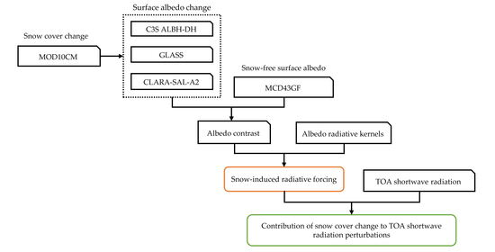
Graphical Abstract

1. Introduction

Snow cover is an integral component of the cryosphere and represents one of the three essential climate variables (ECVs) for snow in the Global Climate Observing System (GCOS) [1], which plays a crucial role in the Earth’s climate system by regulating the surface energy budget [2,3,4]. As a result of the high reflectivity of snow cover, the presence or absence of snow cover plays a key role in the regulation of the heating and cooling patterns of the Earth’s surface, more than any other land surface category. For example, as the surface air temperature increases, the snow cover extent (SCE) retreats and the surface albedo decreases. Consequently, the land surface reflects less solar radiation back to space and retains more energy. The reduced reflected shortwave radiation at the top of the atmosphere (TOA) is known as snow-induced radiative forcing (SnRF) [2,5,6], which is critical for regulating Earth’s energy budget.
As reported by Flanner et al. [2] and Chen et al. [6], SnRF (W m−2) can be calculated by combining observations of SCE, surface albedo contrast (∆α) between snow-covered and snow-free surfaces, and TOA flux variations with surface albedo change (∂F/∂α). The time (t) dependence of SnRF, within a region R (here, the Northern Hemisphere; NH) of area A, can be expressed as Equation (1) [2,5]:
S n RF ( t , R ) = 1 A ( R ) R S ( t , r ) α S ( t , r ) F α ( t , r ) d A ( r ) ,
where S (t, r) is the range of snow cover over the NH; α (t, r) is the surface albedo; ∂α/∂S(t, r) is the rate of variation of the surface albedo with changes in snow cover; and ∂F/∂α(t, r) is the response of the TOA net shortwave radiation anomalies to surface albedo changes. According to Flanner et al. [2] and Chen et al. [6], we assumed that ∂α/∂S and ∂F/∂α were constant for the temporally and spatially varying snow cover S and surface albedo α, respectively. Furthermore, ∂α/∂S could be replaced by the surface albedo contrast ∆α driven by the snow cover anomaly, and ∂F/∂α could be substituted by albedo radiative kernels [2,5,6], wherein the albedo radiative kernels are expressed as the TOA shortwave flux anomalies associated with a 1% change in surface albedo.
The contribution of SCE to the Earth’s energy budget has received substantial attention in recent decades. Several studies have estimated SnRF at regional and global scales. For example, SnRF in snow accumulation and melting seasons over the NH was observed to be 0.01 and 0.12 W m−2 during 1982–2013, respectively [3]. However, SCE reduction was observed to result in the absorption of approximately 0.22 W m−2 extra shortwave radiation in the NH during 1979–2008, which is nearly equal to the radiative forcing caused by Arctic sea ice shrinkage [2]. Similarly, driven by advanced snow end dates, SnRF in the NH was weakened by approximately 0.16 W m−2 from 2001 to 2013 [5]. As per the representative concentration pathway (RCP) 8.5 scenario, a reduction in SCE over the NH may lead to an extra absorption of 0.47–0.60 W m−2 of shortwave radiation in the 21st century [7]. The above-mentioned studies have proved the contribution of SCE to Earth’s radiation budget. However, owing to the uncertainty of input datasets, with a poor quality of the surface albedo dataset, incomplete spatial coverage of snow cover dataset, and short time span of direct TOA radiation observations, significant differences exist in the SnRF estimations from climate models, reanalysis datasets, satellite products, and ground observations. For example, estimates of the SnRF over the NH from the moderate resolution imaging spectroradiometer (MODIS) were approximately 18% lower than the comparable estimates from the coarse-resolution advanced very high resolution radiometer (AVHRR) during 2001–2008 [8]. Moreover, SnRF is a key parameter for the calculation of snow-albedo feedback (SAF), which may have significant effects on climate projection studies. For example, SAF exhibits a five-fold spread across the coupled model intercomparison project phase 5 (CMIP5) models, ranging from 0.03 to 0.16 W m−2 K−1 [9]. In addition, SAF from ground observations is apparently higher than the comparable results from the reanalysis dataset [10]. Therefore, an accurate estimation of SnRF is required for measuring the influence of snow cover on Earth’s radiation budget [2,8], reducing the bias of SAF calculation, and improving climate projections [7,9].
SnRF is determined by several factors, including SCE change, surface albedo anomalies induced by snow cover anomalies (which rely on snow-covered and snow-free surface albedo), solar insolation, and atmospheric states, which determine the propagation of surface albedo changes to the TOA radiation flux [2]. Compared with other variables, snow cover change is the most important driving factor of SnRF. Without snow cover, the ground absorbs approximately four to six times more energy from the sun [11,12]. Instead of a continuous rapid decline in SCE, a recent study reported a notable seasonal divergence of terrestrial SCE across the NH over recent decades [13]. Considering the importance of snow cover for estimating SnRF, quantifying and understanding its spatial and temporal variations is essential for determining its contribution to the Earth’s energy budget.
Optimizing the snow cover and surface albedo inputs utilizing satellite observations is a key approach for improving the accuracy of SnRF [14]. To quantify SnRF and explore its contribution to TOA shortwave radiation anomalies driven by the latest SCE features in the NH, a novel estimation of SnRF using satellite observations at the best achievable spatial and temporal resolutions is urgently required. Therefore, the objective of the present study was two-fold: (1) to quantify the changes in SCE and resulting SnRF; (2) to determine the contribution of SnRF to TOA energy budget anomalies. To achieve these objectives, we first investigated the latest SCE anomalies over the NH. Furthermore, we chose the surface albedo dataset with the best performance resulting from a cross-comparison of SCE changes. Finally, we calculated the SnRF based on the selected surface albedo and explored its spatial distribution and spatial–temporal changes, as well as its influence on the Earth’s energy budget.

2. Materials and Methods

2.1. Materials

To meet the requirements of the SnRF calculation, three variables—snow cover extent, surface albedo, and albedo radiative kernels—were employed in this study.

2.1.1. Snow Cover Extent Dataset

To detect SCE anomalies in the NH and to implement them as input parameters for the estimation of SnRF, a monthly snow chart dataset, calculated from the NH SCE CDR v01r01 [15] and the snow cover range from the MODIS/Terra monthly SCE in 0.05° climate modeling grid (CMG) cells (MOD10CM) [16], were employed in this study.

NHSCE Snow Charts

Monthly snow charts were obtained from the NH SCE CDR v01r01 and utilized to determine the long-term SCE anomaly in the NH from 1972 to 2020. These snow chart data are widely implemented in large-scale SCE anomaly studies, owing to their consistency and long time span [15].

MOD10CM

MOD10CM is an aggregation of MODIS/Terra Snow Cover Daily L3 Global 0.05° CMG (MOD10C1) products [17], providing the monthly mean snow cover percentage in each 0.05° grid cell from February 2000 to the present. The monthly composite of daily MOD10C1 is essential in climate change studies because of the persistent cloudiness and limited spatial coverage of MODIS daily snow cover products, particularly at high latitudes [18]. In this study, MOD10CM was utilized as the snow-cover range in the SnRF calculation.
Compared with other snow cover products, MOD10CM is the only consistent, objective snow cover estimate retrieved from optical satellite observations in the past 20 years with a relatively fine spatial resolution. The 20-year averaged snow cover percentage in the NH calculated from MOD10CM during 2000–2019 is displayed in Figure 1. To match the limited spatial coverage of the surface albedo dataset, high latitudes above 75° N were excluded in this study.

2.1.2. Land Surface Albedo Dataset

The surface albedo, defined as the ratio of the reflected radiation flux to the incoming radiation flux, is one of the most important parameters for calculating SnRF, as it indicates the amount of solar radiation reflected back to space because of snow cover [2,5,7,8,19], and has been further designed as one of the GCOS ECVs [20].
To quantify ∆α, required for estimating SnRF, the broadband directional surface albedo (ALBB-DH) produced by the Copernicus Climate Change Service (C3S) at a spatial resolution of 1 km during 2000–2019 [21] and the MODIS Terra and Aqua combined bidirectional reflectance distribution function (MCD43GF) at a spatial resolution of 1 km during 2001–2017 [22] were implemented in this study. C3S ALBH-DH is the land surface albedo, and MCD43GF is the snow-free surface albedo. Thus, we obtained yearly and monthly ∆α by subtracting MCD43GF from C3S ALBH-DH in the corresponding period.
The broadband directional surface albedo (ALBB-DH) produced by the Copernicus Climate Change Service (C3S) [21] is the best option for surface albedo inputs in SnRF estimation because of its fine spatial resolution (1 km) and complete spatial coverage. However, the C3S ALBH-DH is a newly released dataset. To verify the fitness of C3S ALBH-DH for SnRF estimation, we employed two widely utilized surface albedo datasets, including the global land surface satellite (GLASS) [23] and the Cloud, Albedo, and Surface Radiation datasets from AVHRR data Edition 2 (CLARA-SAL-A2) [24,25] for cross-comparison analysis.

C3S ALBH-DH Surface Albedo Dataset

The C3S ALBH-DH is a global 10-daily gridded surface albedo dataset with a spatial resolution of 1 km covering 1998–2020, calculated from the Systeme Probatoire d’Observation de la Terre-VEGETATION (SPOT-VGT) and the Project for On-Board Autonomy-Vegetation (PROBA-V) [21]. In this study, the integrated black-sky surface albedo computed over the total spectrum (0.4–4.0 µm) from 2000 to 2019 was utilized for analysis. Compared with other surface albedo datasets, such as GLASS, CLARA-SAL-A2, MODIS, the Advanced Polar Pathfinder (APP-X), and the International Satellite Cloud Climatology Project (ISCCP), C3S ALBH-DH is ideal for continental-scale SnRF estimation because of its fine spatial resolution, long time span, and spatial completeness.

GLASS Land Surface Albedo Dataset

The GLASS surface albedo dataset was developed by integrating AVHRR and MODIS version 6 radiance data through a temporal filter scheme [23]. The GLASS surface albedo dataset provides surface albedo at total shortwave, visible, and near-IR spectral ranges under actual atmospheric conditions. To meet the objectives of the present study, 8-day GLASS total shortwave black-sky surface albedo data at a spatial resolution of 0.05°, from 2000 to 2019, were utilized in this study. The GLASS surface albedo dataset has previously been used to quantify the albedo-induced radiative forcing of snow melting over Greenland [26] and snow cover phenology changes over the NH [3,5].

CLARA-SAL-A2 Land Surface Albedo Dataset

The CLARA-SAL-A2 surface albedo dataset was generated based on a homogenized AVHRR radiance time series and was created using algorithms to derive surface albedo for different land use types, including snow, sea ice, open water, and vegetation. Currently, CLARA-SAL-A2 is the only available long-time-span surface albedo product that is completely dependent on AVHRR imagery [24,25]. For the purpose of the present study, the monthly means of CLARA-SAL-A2 at a spatial resolution of 0.25° from 2000 to 2019 were employed in the analysis.

MCD43GF Snow-Free Surface Albedo Dataset

To obtain the climatology of monthly mean snow-free surface albedo required in SnRF estimation, a global gap-filled snow-free surface albedo dataset retrieved from the MODIS Terra and Aqua combined bidirectional reflectance distribution function (MCD43GF) at a spatial resolution of 1 km during 2001–2017 [22] was utilized in this study. MCD43GF provides spatially complete surface albedo values after removing the presence of snow cover, which are computed by MODIS spectral bands 1–7, as well as shortwave infrared, visible, and near-infrared bands. For the present study, the daily broadband snow-free black-sky surface albedo data from 2001 to 2017 were used.

2.1.3. Albedo Radiative Kernels Datasets

The albedo radiative kernel, expressed as the TOA shortwave flux anomaly associated with a 1% change in surface albedo, is a key input variable for estimating SnRF. Compared with analytical models, the radiative kernel approach has significant advantages in separating the radiative responses to land surface albedo induced by snow cover changes from other climate parameters, enhancing the accuracy for capturing the functional dependence of planetary albedo on surface albedo [9].
To reduce uncertainties in SnRF estimation, three albedo radiative kernels, the National Center For Atmospheric Research (NCAR) Community Atmosphere Model 3 (CAM3) gridded at a horizontal resolution of 2.81° [27], the Geophysical Fluid Dynamics Laboratory (GFDL) Atmospheric Model 2 (AM2) gridded at a horizontal resolution of 2.50° [28], and the sixth generation atmospheric general circulation model (ECHAM6) gridded at a horizontal resolution of 1.875° [29], were used in this study. The intra-annual variability of the three albedo radiative kernels is displayed in Figure 2.

2.1.4. TOA Radiation Budget Dataset

To explore the contribution of SnRF to TOA energy budget anomalies, the clear-sky upward TOA shortwave (0.2–5 µm) flux, retrieved from the Clouds and Earth’s Radiant Energy Systems (CERES) Energy Balanced and Filled (EBAF) products [30] at a spatial resolution of 1.0°, from 2000 to 2019, was implemented. The CERES EBAF clear-sky shortwave flux is spatially complete, and is inferred from both CERES and MODIS measurements conducted monthly [31].

2.1.5. Data Preparation

A summary of the datasets implemented in this study is presented in Table 1. To cater to the requirements of the SnRF calculation, the snow cover range, land surface albedo, and albedo radiative kernels were regridded at a spatial resolution of 0.05° using the gdalwarp reprojection and warping utility (https://gdal.org/programs/gdalwarp.html, acessed on 28 November 2021).
For datasets with a spatial resolution coarser than 0.05°, we used “cubicspline” in the resampling process; for datasets with spatial resolution finer than 0.05°, we utilized “average” in the resampling process, which computes the weighted average of all contributing pixels (excluding NODATA) at 0.05°. Moreover, to match the temporal resolution (monthly) of albedo radiative kernels, both the 10-day C3S-ALBH-DH and daily MCD43GF were reproduced to generate monthly mean values.

2.2. Methods

2.2.1. Z-Score Normalization

Z-score normalization was implemented to normalize the different variables in the cross-comparison analysis. For variable X, the Z-score (Zx) was calculated using Equation (2) [32].
Z x = X μ x δ x ,
where μx is the average value of X and δx is the standard deviation of X.

2.2.2. Linear Slope

The linear slope measures the rate of change in the dependent variable as the independent variable changes, which can be calculated using Equation (3):
Slope = Δ y Δ x ,
where ∆y is the change in dependent variable y and ∆x is the change in independent variable x.

2.2.3. Pearson Correlation Coefficient

The Pearson correlation coefficient (r) was utilized to quantify the degree of correlation between two variables. For variables X and Y, r was calculated using Equation (4):
r x , y = cov ( x , y ) δ x δ y ,
where cov(x, y) is the covariance of variable x and variable y; δx is the standard deviation of variable x; and δy is the standard deviation of variable y.

2.2.4. Relative Contribution Calculation

We assumed that the variability in the annual mean SnRF was attributed to SnRF anomalies in each month. Furthermore, regression analysis was utilized to quantify the contribution of SnRF in each month to the annual mean SnRF variability during 2000–2019 using Equation (5):
S n RF z = i = 1 m β i × S n RF iz + ε ,
where SnRFz is the Z-score of the normalized annual mean SnRF during 2000–2019; SnRFiz is the Z-score normalized SnRF in month i (i = 1, 12); βi is the regression coefficient for SnRFiz; and ε is the residual error.
Furthermore, the relative contribution (Ci) of SnRFiz to SnRFz was confirmed using Equation (6):
C i = | β i × X i z _ s l o p e | | β 1 × S n RF 1 z _ slope | + | β 2 × S n RF 2 z _ slope | + + | β 12 × S n RF 12 z _ slope | ,
where SnRFiz_slope is the linear slope of SnRFiz, which can be calculated using Equation (3).
The regression analysis is an effective approach for solving collinearity problems in contribution analysis [33] and has been applied in gross primary production trend analysis in the Three-North region of China [34], as well as for determining the interannual evapotranspiration sensitivity to climate change across the Yellow River basin [35].

3. Results

To explore the contribution of changes in SCE to TOA shortwave radiation perturbation in the NH, we first investigated the SCE anomalies during 2000–2019. Further, we verified the performance of the C3S surface albedo through a cross-comparison with the snow cover dataset. Finally, we calculated the variabilities of the annual mean SnRF and identified the dominant month that controlled the annual mean SnRF.

3.1. Characteristic of SCE Variability in the NH during 2000–2019

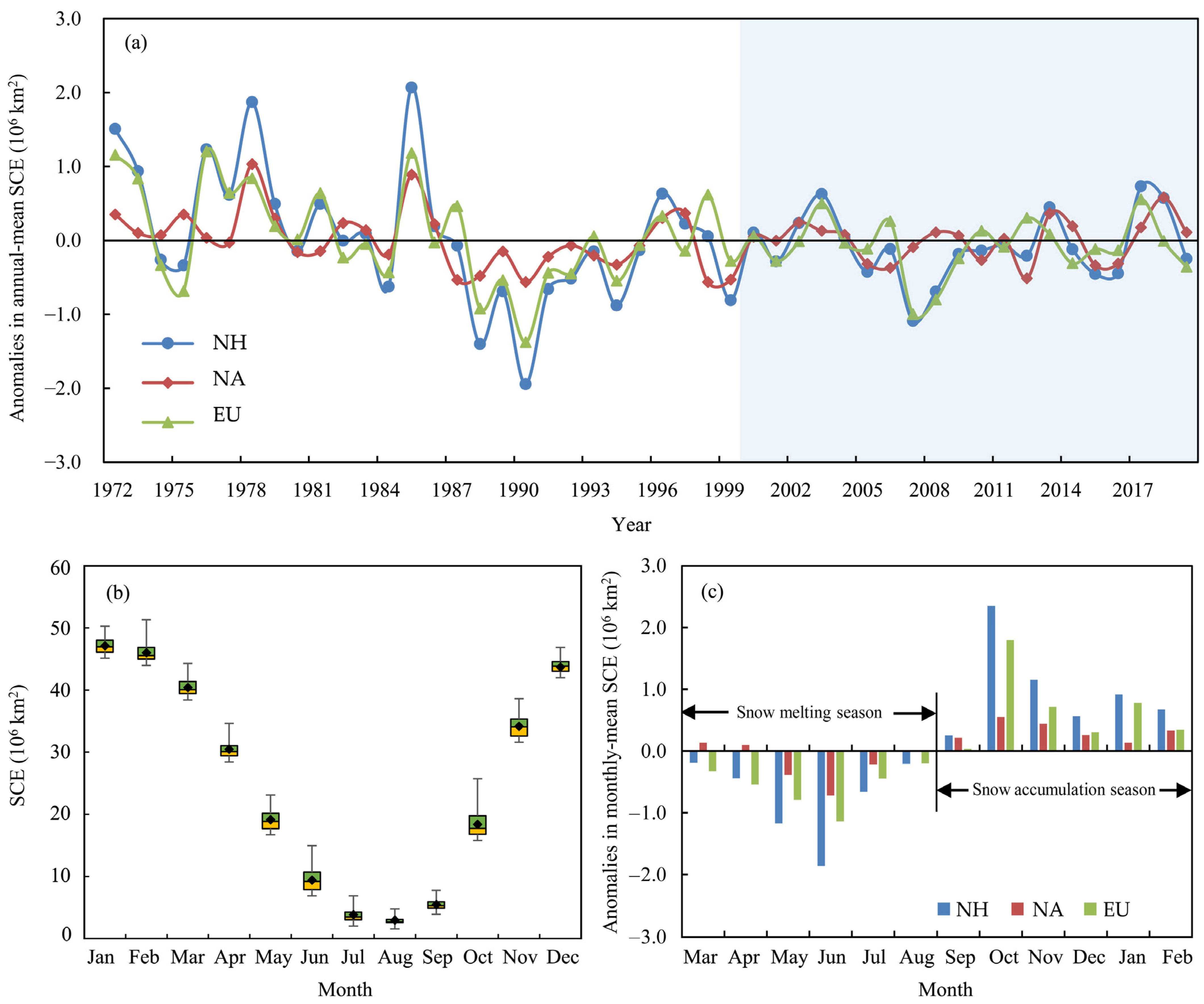
The Z-score anomalies of annual mean SCE in the NH, including North America (NA) and Eurasia (EU), are displayed in Figure 3a. The climatology of SCE in each month and the associated changes during 2000–2019 are exhibited in Figure 3b,c, respectively. Changes were calculated by the monthly mean SCE during 2000–2019 minus the comparable values in the referencing period, 1972–2000.
As displayed in Figure 3a, the well-documented rapid SCE decline over the NH since the late 1960s [36,37,38] has experienced a hiatus in recent years, especially during 2000–2019, both in NA and EU. The SCE in the NH declined at a speed of −0.52 × 10⁶ km2 per decade (p < 0.05) during 1972–2000, but displayed negligible changes during 2000–2019. The ignorable SCE anomalies from 2000 to 2019 disagree with climate projections, wherein the SCE will continue to shrink in the future [37,39,40].
The seasonal variability of SCE in the NH is presented in Figure 3b. The maximum SCE in the NH occurred in January (47.78 ± 1.59 106 km2) during 2000–2019. Meanwhile, the minimum SCE in the NH occurred in August (2.59 ± 0.63 106 km2) during the same period. Based on the seasonal cycle of SCE, and published studies, such as those by Chen et al. [13] and Brutel-Vuilmet et al. [41], the months from March to August were defined as the snow melting season and the months from September to February were the snow accumulation season. Detailed SCE changes per month further revealed that, in comparison with 1972–2000, SCE anomalies between accumulation and melting seasons were markedly different during 2000–2019 (Figure 3c). In the melting season, SCE in the NH declined from 1.86 × 10⁶ km2 in June to 0.19 × 10⁶ km2 in March. Conversely, SCE increased in the accumulation season over the NH during the same period, ranging from 0.26 × 10⁶ km2 in September to 2.35 × 10⁶ km2 in October. The distinct SCE anomalies in each month indicate that, instead of a rapid SCE decline, the intra-annual SCE variability is a new characteristic of snow cover in recent years.

3.2. Validation of C3S Surface Albedo Dataset in SnRF Calculation

A cross-comparison was conducted for SCE and surface albedo anomalies between March and June, which presented the minimum and maximum negative changes in SCE over the NH during 2000–2019.

3.2.1. Performance of C3S ALBH-DH in March during 2000–2019

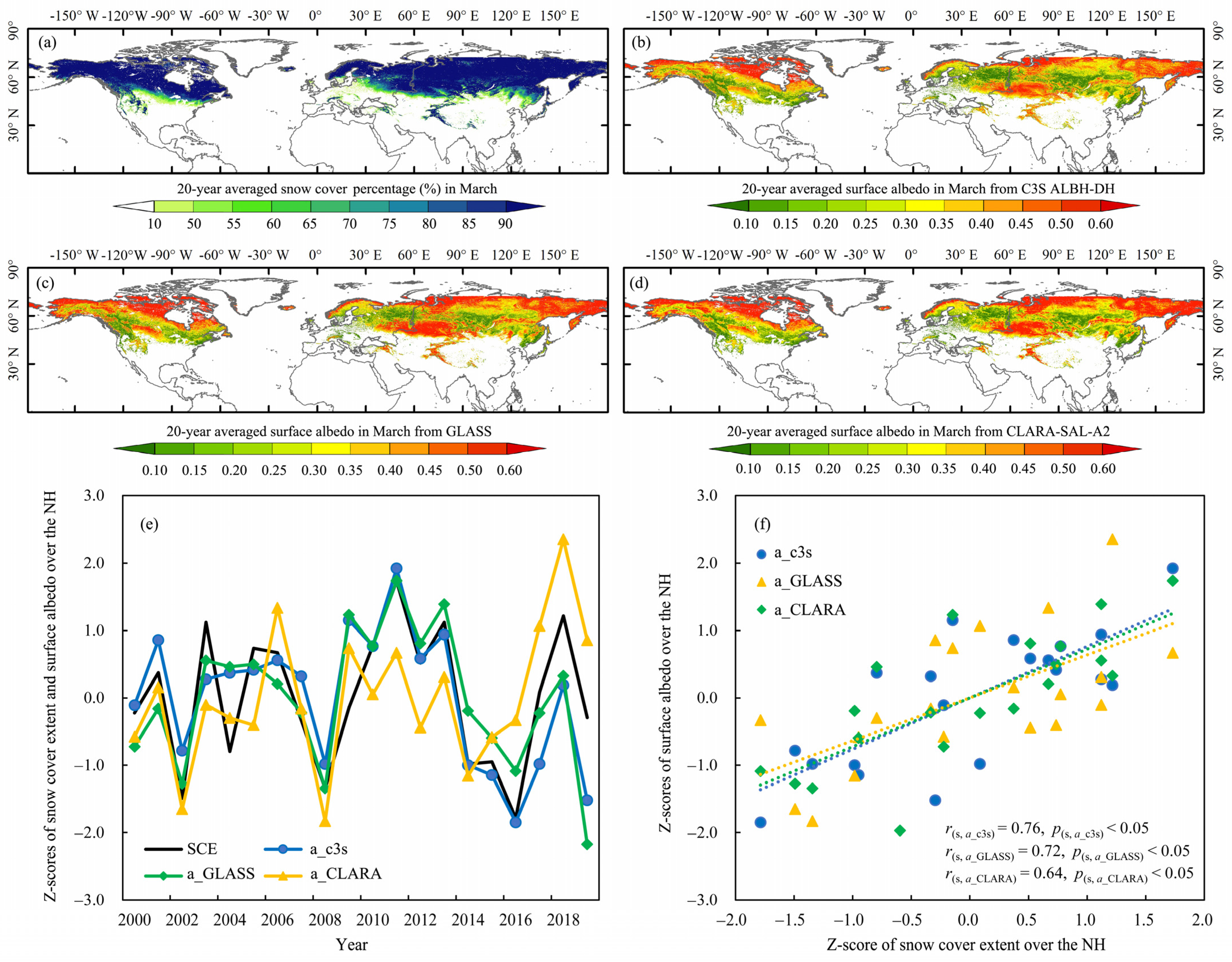
The 20-year averaged March snow cover percentage and surface albedo from C3S ALBH-DH, GLASS, and CLARA-SAL-A2 during 2000–2019 are displayed in Figure 4.
As displayed in Figure 4a, the snow cover percentage in March presented a clear latitudinal distribution from low to high latitudes. Compared with the snow cover percentage, the surface albedo in March exhibited substantial spatial variability, as satellite-retrieved broadband surface albedo combined snow cover and other surface (mostly vegetation) within the same grid cell. Moreover, the 20-year averaged surface albedo in March from C3S ALBH-DH (Figure 4b), GLASS (Figure 4c), and CLARA-SAL-A2 (Figure 4d) displayed similar spatial distributions. In addition, the snow cover and surface albedo exhibited similar peaks and valleys from 2000 to 2019 (Figure 4e), with peaks occurring in 2011 and 2018, corresponding to the extremely low temperature and heavy snowfall induced by the Arctic Oscillation event [42,43].
The Z-scores of SCE for March and surface albedo from C3S ALBH-DH, GLASS, and CLARA-SAL-A2, and linear scatter plots between the Z-scores of SCE for March and surface albedo during 2000–2019 are displayed in Figure 4e,f, respectively. The performance of surface albedo is largely determined by its spatial resolution. Compared with GLASS (r = 0.72, p < 0.05) and CLARA-SAL-A2 (r = 0.64, p < 0.05), C3S ALBH-DH (r = 0.76, p < 0.05) displayed an improved linear correlation coefficient with SCE during 2000–2019 (Figure 4f). This indicates that C3S ALBH-DH skillfully captured the SCE variability and performed better than GLASS and CLARA-SAL-A2 during 2000–2019. Moreover, uncertainty in snow cover data [36,37] and changes in snow morphology [44] may reduce its correlation with surface albedo. However, C3S ALBH-DH still captured SCE anomalies in March during 2000–2019.

3.2.2. Performance of C3S-ALBH-DH in June during 2000–2019

The 20-year average snow cover percentage in June and the surface albedo from C3S ALBH-DH, CLARA-SAL-A2, and GLASS from 2000 to 2019 are exhibited in Figure 5.
The SCE in June decreased nearly twice as rapidly as the widely acknowledged sea ice extent shrinking in September during 1979–2011 [38] and exhibited a sustained rapid decrease during 2000–2019 (Figure 3c). To verify the ability of C3S ALBH-DH at capturing the rapid SCE decline in June, we first investigated the spatial distribution of the snow cover percentage and surface albedo in June. Further, we calculated the correlation coefficient between changes in the SCE and surface albedo in June during 2000–2019.
As shown in Figure 5a, snow cover in June was mostly distributed at high latitudes in NA and EU. Meanwhile, the surface albedo from C3S ALBH-DH (Figure 5b), GLASS (Figure 5c), and CLARA-SAL-A2 (Figure 5d) in snow-covered regions exhibited similar spatial distributions. Driven by the SCE decline in June (−1.8992 × 10⁶ km2 decade−1, p < 0.01), the June surface albedo from C3S ALBH-DH, CLARA-SAL-A2, and GLASS demonstrated similar decreasing trends of 0.0732 decade−1 (p < 0.01), 0.0725 decade−1 (p > 0.05), and 0.0505 decade−1 (p > 0.05), respectively. Compared with C3S ALBH-DH, changes in surface albedo from both CLARA-SAL-A2 and GLASS were not significant at the 5% level. Meanwhile, the linear correlation coefficient between C3S ALBH-DH surface albedo and SCE in June was 0.49 (p < 0.05) during 2000–2019. Although positive correlation coefficients with SCE were also observed using GLASS (r = 0.48, p < 0.05) and CLARA-SAL-A2 (r = 0.39, p > 0.05), C3S ALBH-DH performed better in terms of representing the June snow cover decline in the NH during 2000–2019.

3.3. Estimation of SnRF over the NH

Applying the albedo radiative kernel approach using Equation (1), we first calculated the SnRF during 2000–2019. Further, we compared the SnRF estimates with direct TOA shortwave flux observations and explored the relative contribution from each month to the annual mean SnRF from 2000 to 2019.

3.3.1. Estimated SnRF over the NH during 2000–2019

The spatial distributions of the 20-year annual mean SnRF in the NH under clear-sky conditions, and the changes that occurred during 2000–2019, are displayed in Figure 6a,b. The intra-annual cycles of SnRF in the NH during 2000–2019 are displayed in Figure 6d. Changes in SnRF were expressed as linear trends multiplied by the time interval, following Flanner et al. [2].
The 20-year annual mean SnRF in NH was estimated to be −1.13 (±0.05) W m−2 from 2000 to 2019 (Figure 6a,c), with high values of SnRF distributed at high latitudes in NA and EU, the Pamir Mountains, and East Siberia. Moreover, the change in SnRF over the NH was estimated to be −0.1033 (± 0.0081) W m−2 from 2000 to 2019. The absolute value of SnRF is decreasing, indicating a generally receding trend of radiative cooling in the NH from 2000 to 2019. Meanwhile, the minima of annual mean SnRF occurred in 2009 and 2011, coinciding with the large-scale El Niño and Arctic Oscillation events, particularly in 2009 [42]. Conversely, the peaks occurred in 2015 and 2019, corresponding to La Niña and extremely high temperatures [45].
The intra-annual cycles of SnRF in the NH during 2000–2019 indicated that the SnRF peaks at approximately −3.83 (± 0.14) W m−2 in April, when both solar irradiance and SCE over the NH are high. Compared with the SnRF in the NH during 1979–2008 [2], the peak of SnRF was much lower. The detailed SnRF anomalies in each month revealed that SnRF significantly decreased from February to June, indicating a weakened radiative cooling effect over the NH during these months in 2000–2019. The most significant SnRF decline occurred in May at 0.3681 W m−2 (p < 0.01) from 2000 to 2019. Meanwhile, SnRF weakened by 0.1714 W m−2 (p < 0.01) in June and 0.1559 W m−2 (p < 0.05) in March. Conversely, SnRF exhibits negligible changes in snow accumulation months, especially in October, November, January, and February. The contrasting SnRF changes in snow accumulation and melting seasons may lead to unbalanced intra-annual shortwave radiative distribution, which should be considered in climate change projections.

3.3.2. Direct Estimates of TOA Shortwave Flux Anomalies

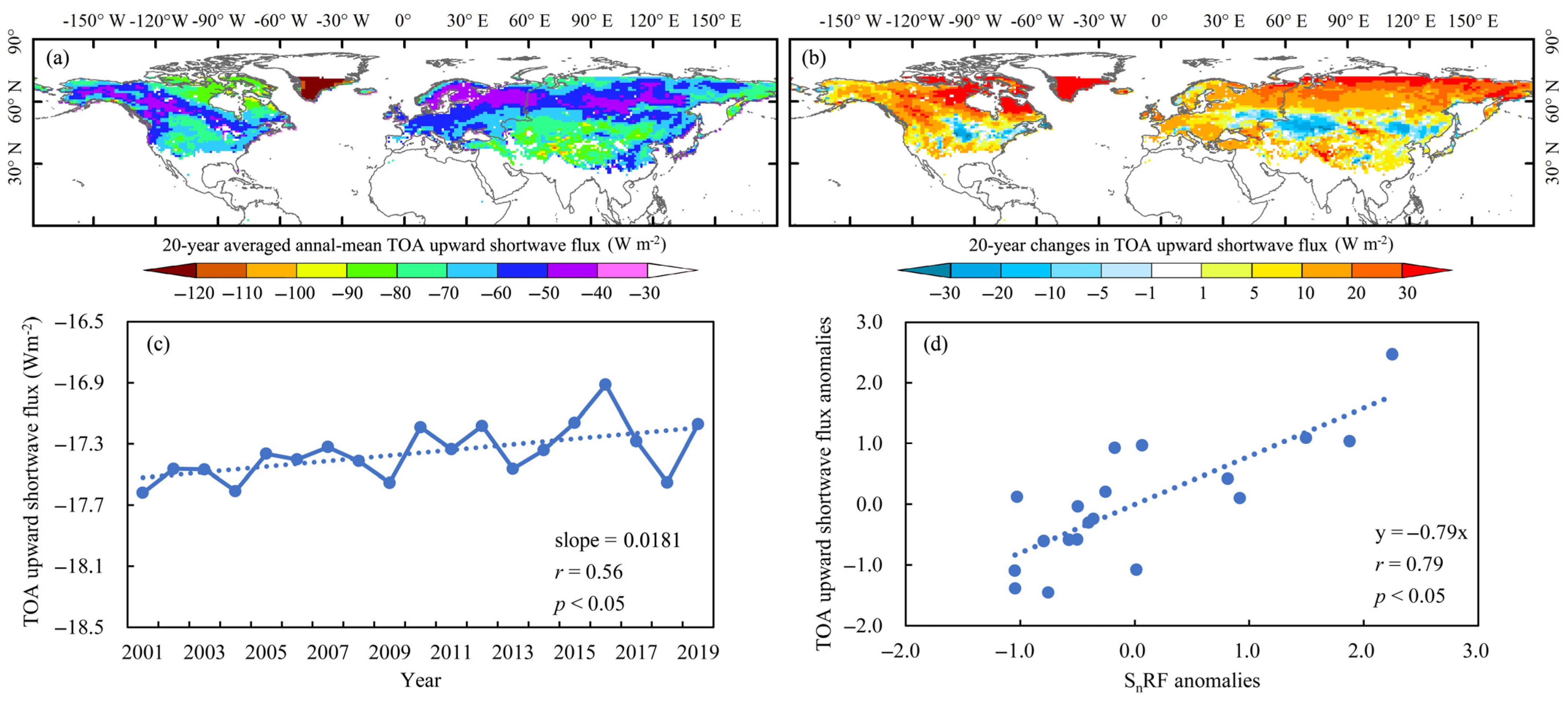
The 20-year averaged annual mean TOA shortwave flux and changes calculated from CERES EBAF observations from 2000 to 2019 are displayed in Figure 7a,b. The variability of annual mean TOA upward shortwave flux and its linear correlation with SnRF are exhibited in Figure 7c,d, respectively. To match the SnRF definition, an upwelling flux was defined as negative in the present study.
The observed annual mean TOA upward shortwave flux changes (Figure 7b) were highly consistent, both spatially and temporally, with SnRF anomalies (Figure 6b) across the NH during 2000–2019. Similar to SnRF, the TOA upward shortwave flux increased at high latitudes in NA and EU, indicating less TOA shortwave flux back to space and more shortwave radiation absorption by the Earth climate system from 2000 to 2019. In comparison, the TOA upward shortwave flux was enhanced in the mid-latitudes of Central Asia, northeastern China, and Central United States during 2000–2019, which agrees with previous findings of large scale cold snaps, heavy snowfall, and glacier events across the United States, Europe, and East Asia, and the observed long-term large-scale cooling trends for land surface temperature in winter over at mid-latitudes [46,47]. Meanwhile, the interannual variability of the annual mean TOA upward shortwave flux increased at a rate of 0.181 Wm−2 decade−1 (p < 0.05), which is consistent with the estimated SnRF anomalies during the same period (Figure 6c). The correlation coefficient between the SnRF and TOA upward shortwave flux in the NH was 0.79 (p < 0.05), highlighting the contribution of SnRF to TOA upward shortwave anomalies in the NH from 2000 to 2019. The strong correlation between SnRF and TOA upward shortwave flux indicates that changes in SnRF may further influence and control the local and regional energy budgets owing to climate change.

3.3.3. Attribution of SnRF Anomalies over the NH during 2000–2019

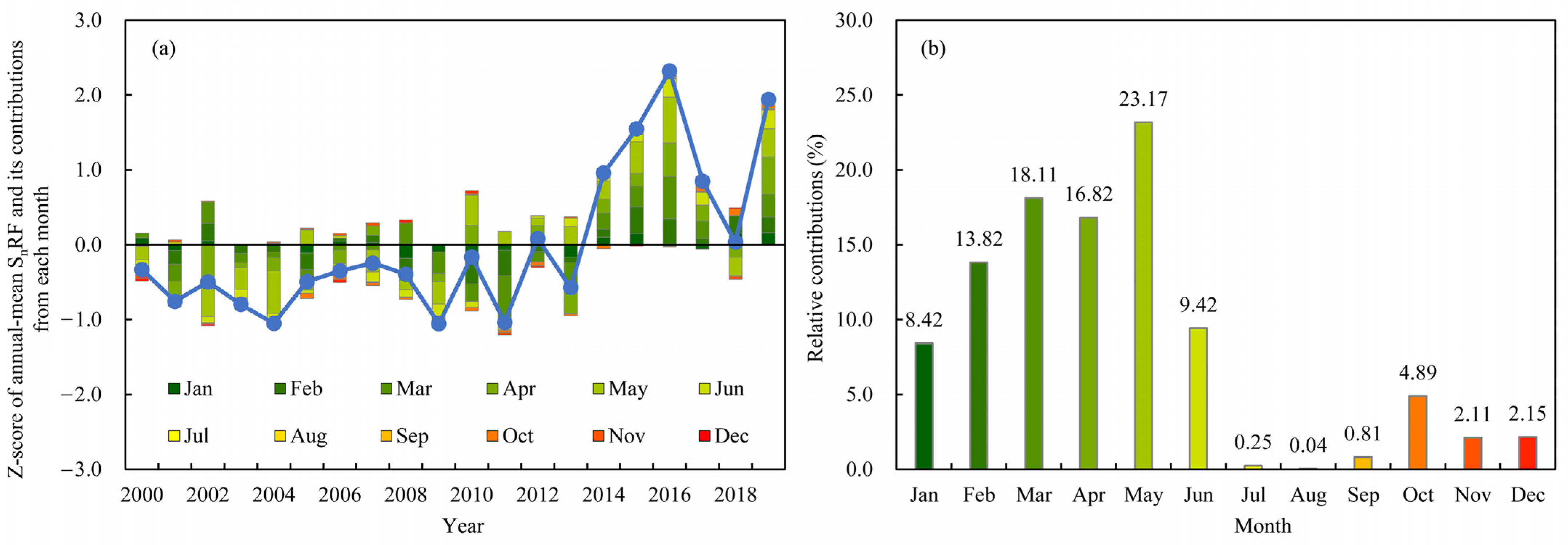
Changes in the annual mean SnRF could be positively represented by SnRF every month by utilizing a multiple linear regression equation with different coefficients, as displayed in Equation (5). To attribute the annual mean SnRF changes and explore the dominant month that controlled the annual mean SnRF, we calculated the relative contribution of SnRF in each month to the annual mean SnRF anomalies over the NH from 2000 to 2019. Applying a ridge regression analysis with Equation (5), the relative contribution of SnRF in each month to the annual mean SnRF anomalies over the NH during 2000–2019 was calculated, as displayed in Figure 8.
The Z-score of the annual mean SnRF over the NH during 2000–2019 is displayed in Figure 8a. The resulting contributions from the SnRF in each month to the annual mean SnRF anomalies were significantly different, wherein the SnRF in melting seasons controlled the annual mean SnRF variability from 2000 to 2019. Detailed 20-year averaged relative contributions from each month to the annual mean SnRF anomalies (Figure 8b) further revealed that May accounted for 23.17% of the annual mean SnRF variability over the NH, followed by March (18.11%) and April (16.82%) during 2000–2019. The SnRF in accumulation seasons contributed insignificantly towards the annual mean SnRF from 2000 to 2019. Although the SCE over the NH significantly increased in October (Figure 3a), the SnRF in October remained low because of low insolation during that month.
Based on the results of SCE and SnRF anomalies over the NH, we inferred that the annual mean SnRF over the NH exhibited a continuous weakening trend from 2000 to 2019, despite the negligible changes in the annual mean SCE. With a rapid SCE decline in snow melting seasons, the SnRF weakened during the melting seasons, especially in May. Conversely, although SCE increased in accumulation seasons, the low insolation and solar incidence angle led to a low SnRF, contributing little to the annual mean SnRF.

4. Discussion

Snow-induced radiative forcing SnRF quantitatively estimates the influence of snow on the energy balance of the Earth–atmosphere system and reflects the importance of snow in the mechanism of potential climate change. Therefore, estimating the SnRF is valuable for climate change and climate projections studies. Consequently, quantifying the SnRF and providing support for accurate simulations of the climate change response were the major objectives of the present study.
Previous studies have proved that SCE in the NH has experienced a rapid decrease since satellite observations began in the late 1960s [3,36,37,38]. Climate projections suggest that the SCE will continue shrinking in the future [37,39], coincident with hemispheric warming, indicating the positive feedback of surface reflectivity on climate [2,36,37]. Differently to the SCE projections, the rapid SCE decline over the NH has experienced a hiatus in recent years, especially during 2000–2019. Therefore, novel investigations into SCE variability and its contribution to the Earth energy budget are necessary. Due to the limited spatial coverage of the surface albedo dataset, high latitudes above 75° N were excluded in this study.
The method utilized in this study is appropriate for optimizing the input parameters (e.g., snow cover, surface albedo, and albedo radiative kernels) in SnRF calculations to enhance climate change studies and climate projections in the NH. Although we employed the best achievable satellite observations, several issues and limitations exist. Unlike previous research, this study utilized C3S ALBH-DH in SnRF estimation, which provides a better correlation coefficient with SCE anomalies, both in March and June, during 2000–2019. Using C3S ALBH-DH in SnRF estimation greatly reduced the uncertainty in the SnRF calculation induced by surface albedo biases that exist at coarser spatial resolution, such as in GLASS [5] and MODIS [2,7]. To verify the performance of the C3S ALBH-DH climate studies, we utilized GLASS and CLARA-SAL-A2 for a comparison. As CLARA-SAL-A2 solely provides black-sky surface albedo (integration of the bidirectional reflectance distribution function over the viewing hemisphere), the cross-comparison analysis focused on this. Consequently, SnRF in this study only represents the shortwave (solar spectrum) component of the snow-induced radiative forcing. However, compared with SnRF using white-sky surface albedo (integration of the directional albedo over the illumination hemisphere), the comparable value using black-sky surface albedo has a slightly larger value of 4.32% [2,9]. As the difference between black-sky and white-sky surface albedo is systematic, this difference is not likely to influence the spatial and temporal changes in SnRF.
The albedo radiative kernel approach facilitates the estimation of SnRF in this study. However, unsolved spectral variations were excluded from this study. Snow induces a greater albedo contrast in the visible region than that in the near-infrared region, whereas the albedo radiative kernels are generated with spectrally uniform surface albedo perturbations, and with spectrally varying surface fluxes. A sensitivity analysis by Flanner et al. [2] observed that unsolved spectral variations may result in a 5% difference between the results from the entire broadband and separate components. Thus, the excluded unresolved spectral variations in the radiative kernel technique did not influence the major conclusions of our study.
Except for SnRF in clear-sky conditions, the comparable results in all-sky conditions also require further attention. However, published studies using both all-sky and clear-sky albedo radiative kernels have reported that the all-sky SnRF exhibits similarly inter-annual, intra-annual, and spatial pattern variabilities to clear-sky SnRF, except for a 30% difference in magnitude [2,11,48]. Therefore, this study solely utilized clear-sky albedo radiative kernels in SnRF calculation, which is not likely to influence the major conclusions of this study.

5. Conclusions

Based on satellite observations, this study explored the latest SCE changes over the NH, quantified SnRF, and determined its influence on TOA shortwave anomalies from 2000 to 2019. These results provide insights into the role of snow cover in the Earth’s climate system in the context of climate change.
A hiatus in the rapid decline of SCE has been observed in recent years, especially during 2000–2019. In this study, detailed SCE analysis in each month revealed contrasting SCE anomalies between the accumulation and melting seasons over the NH during 2000–2019 compared with those during 1972–2000. A cross-comparison between the snow cover percentage and three surface albedo values in March and June, namely those from C3S ALBH-DH, CLARA-SAL-A2, and GLASS, from 2000 to 2019, demonstrated the reliability of C3S ALBH-DH for estimating SnRF. Compared with GLASS (r = 0.72, p < 0.05) and CLARA-SAL-A2 (r = 0.64, p < 0.05), the C3S ALBH-DH (r = 0.76, p < 0.05) displayed a better linear correlation coefficient with snow cover percentage in March. Meanwhile, the performance of C3S ALBH-DH (0.49, p < 0.05) in June was better than that of GLASS (r = 0.48, p < 0.05) and CLARA-SAL-A2 (r = 0.39, p > 0.05) during 2000–2019.
Utilizing the MOD10CM snow cover range, C3S ALBH-DH surface albedo, and three albedo radiative kernels, this study estimated the SnRF from 2000 to 2019. The 20-year annual mean SnRF in the NH was estimated to be −1.13 (±0.05) W m−2 from 2000 to 2019. Meanwhile, changes in SnRF during 2000−2019 were estimated to be 0.094 (±0.0081) W m−2, indicating a generally weakening trend of radiative cooling over the NH. The coefficient of determination between SnRF and the TOA upward shortwave flux over the NH from 2000 to 2019 was 0.79 (p < 0.05), highlighting the contribution of SnRF to TOA upward shortwave anomalies over the NH. In addition, the ridge regression analysis revealed that SnRF in the snow accumulation seasons dominated the annual mean SnRF variability over the NH during 2000–2019. May accounted for the greatest (23.17%) annual mean SnRF variability over the NH, followed by March (18.11%) and April (16.82%).
A generalized analysis observed that, although the annual mean SCE exhibited negligible changes from 2000 to 2019, the notable seasonal SCE changes led to a continuous weakening of SnRF over the NH, which should be considered when performing climate projection studies. Therefore, the results presented in this study are beneficial for climate change studies. Owing to the continuous seasonal variability and spatial heterogeneity of SCE in the NH, the monitoring, modeling, and prediction of SnRF are urgently required to reduce their bias in climate projections and CMIP models.

Author Contributions

Conceptualization, X.C. and Y.Y.; methodology, X.C.; software, C.Y.; validation, X.C. and C.Y.; formal analysis, X.C.; investigation, C.Y. and X.C.; resources, X.C.; data curation, X.C. and C.Y.; writing—original draft preparation, X.C.; writing—review and editing, X.C. and C.Y.; visualization, X.C.; supervision, Y.Y.; project administration, Y.Y.; funding acquisition, X.C. All authors have read and agreed to the published version of the manuscript.

Funding

This work was jointly supported by the National Natural Science Foundation of China (No.42001377), the comprehensive survey of biodiversity over the Mongolian Plateau (No.2019FY102001), the National Earth System Science Data Sharing Infrastructure (No.2005DKA32300), and the 13th Five-year Informatization Plan of Chinese Academy of Sciences, Construction of Scientific Data Center System (No. WX145XQ07-11).

Institutional Review Board Statement

Not applicable.

Informed Consent Statement

Not applicable.

Data Availability Statement

The snow cover data presented in this study are openly available in Estilow et al. [15] at https://climate.rutgers.edu/snowcover/ (accessed on 15 January 2020) and Riggs and Hall [17] at https://doi.org/10.5067/MODIS/MOD10CM.006 (accessed on 1 September 2020); The C3S ALBH-DH surface albedo dataset [21] is openly available at https://cds.climate.copernicus.eu (accessed on 1 September 2020); the CLARA-SAL-A2 surface albedo dataset [25] is available at https://doi.org/10.5676/EUM_SAF_CM/CLARA_AVHRR/V002_01 (accessed on 15 September 2020); the GLASS surface albedo dataset [23] is openly available at http://glass.umd.edu/Albedo/MODIS/0.05D/ (accessed on 15 September 2020); the MCD43GF snow-free surface albedo dataset [22] is openly available at https://doi.org/10.5067/MODIS/MCD43GF.006 (accessed on 1 June 2020); the albedo radiative kernels are openly available in Soden et al. [28] at https://climate.rsmas.miami.edu/data/radiative-kernels/ (accessed on 30 June 2020), Mauritsen et al. [29] at https://climatedataguide.ucar.edu/climate-data/radiative-kernels-climate-models (accessed on 30 June 2020), and Shell et al. [27] at http://people.oregonstate.edu/~shellk/kernel.html (accessed on 30 June 2020).

Acknowledgments

We gratefully acknowledge the anonymous reviewers for their constructive comments and suggestions. In addition, we would like to thank the data sharing agencies for making the datasets used in this study available.

Conflicts of Interest

The authors declare no conflict of interest. The founding sponsors had no role in the design of the study; in the collection, analyses, or interpretation of data; in the writing of the manuscript, and in the decision to publish the results.

References

  1. GCOS. Snow: Essential Climate Variable (ECV) Factsheet. 2019. Available online: https://gcos.wmo.int/en/essential-climate-variables/snow/ (accessed on 15 September 2020).
  2. Flanner, M.G.; Shell, K.M.; Barlage, M.; Perovich, D.K.; Tschudi, M.A. Radiative forcing and albedo feedback from the Northern Hemisphere cryosphere between 1979 and 2008. Nat. Geosci. 2011, 4, 151–155. [Google Scholar] [CrossRef]
  3. Chen, X.; Liang, S.; Cao, Y. Satellite observed changes in the Northern Hemisphere snow cover phenology and the associated radiative forcing and feedback between 1982 and 2013. Environ. Res. Lett. 2016, 11, 084002. [Google Scholar] [CrossRef]
  4. Thackeray, C.W.; Fletcher, C.G. Snow albedo feedback: Current knowledge, importance, outstanding issues and future directions. Prog. Phys. Geogr. 2016, 40, 392–408. [Google Scholar] [CrossRef]
  5. Chen, X.; Liang, S.; Cao, Y.; He, T.; Wang, D. Observed contrast changes in snow cover phenology in northern middle and high latitudes from 2001–2014. Sci. Rep. 2015, 5, 16820. [Google Scholar] [CrossRef] [Green Version]
  6. Chen, X.; Liang, S.; Yang, Y. Differences in snow-induced radiative forcing estimated from satellite and reanalysis surface albedo datasets over the Northern Hemisphere landmass for the overlapping period of 1982–2012. Environ. Res. Commun. 2020, 2, 091001. [Google Scholar]
  7. Perket, J.; Flanner, M.G.; Kay, J.E. Diagnosing shortwave cryosphere radiative effect and its 21st century evolution in CESM. J. Geophys. Res. Atmos. 2014, 119, 1356–1362. [Google Scholar] [CrossRef] [Green Version]
  8. Singh, D.; Flanner, M.G.; Perket, J. The global land shortwave cryosphere radiative effect during the MODIS era. Cryosphere 2015, 9, 2057–2070. [Google Scholar] [CrossRef] [Green Version]
  9. Qu, X.; Hall, A. On the persistent spread in snow-albedo feedback. Clim. Dyn. 2014, 42, 69–81. [Google Scholar] [CrossRef]
  10. Wegmann, M.; Dutra, E.; Jacobi, H.-W.; Zolina, O. Spring snow albedo feedback over northern Eurasia: Comparing in situ measurements with reanalysis products. Cryosphere 2018, 12, 1887–1898. [Google Scholar] [CrossRef] [Green Version]
  11. Chen, X.; Long, D.; Hong, Y.; Liang, S.; Hou, A. Observed radiative cooling over the Tibetan Plateau for the past three decades driven by snow-cover-induced surface albedo anomaly. J. Geophys. Res. Atmos. 2017, 122, 6170–6185. [Google Scholar] [CrossRef]
  12. NSIDC. State of the Cryosphere: Northern Hemisphere Snow. 2019. Available online: https://nsidc.org/cryosphere/sotc/snow_extent.html (accessed on 15 September 2020).
  13. Chen, X.; Yang, Y.; Ma, Y.; Li, H. Distribution and Attribution of Terrestrial Snow Cover Phenology Changes over the Northern Hemisphere during 2001–2020. Remote Sens. 2021, 13, 1843. [Google Scholar] [CrossRef]
  14. Fernandes, R.; Zhao, H.; Wang, X.; Key, J.; Qu, X.; Hall, A. Controls on Northern Hemisphere snow albedo feedback quantified using satellite Earth observations. Geophys. Res. Lett. 2009, 36, L21702. [Google Scholar] [CrossRef] [Green Version]
  15. Estilow, T.W.; Young, A.H.; Robinson, D.A. A long-term Northern Hemisphere snow cover extent data record for climate studies and monitoring. Earth Syst. Sci. Data 2015, 7, 137–142. [Google Scholar] [CrossRef] [Green Version]
  16. Hall, D.K.G.; Riggs, G.A. MODIS/Terra Snow Cover Monthly L3 Global 0.05 Deg CMG, Version 6. NASA National Snow and Ice Data Center Distributed Active Archive Center. 2015. Available online: https://doi.org/10.5067/MODIS/MOD10CM.006 (accessed on 15 September 2020).
  17. Riggs, G.A.; Hall, D.K. MODIS Snow Products Collection 6 User Guide. 2015. Available online: https://modis-snow-ice.gsfc.nasa.gov/uploads/C6_MODIS_Snow_User_Guide.pdf (accessed on 15 September 2020).
  18. Frei, A.; Tedesco, M.; Lee, S.; Foster, J.; Hall, D.K.; Kelly, R.; Robinson, D.A. A review of global satellite-derived snow products. Adv. Space Res. 2012, 50, 1007–1029. [Google Scholar] [CrossRef] [Green Version]
  19. Groisman, P.Y.; Karl, T.R.; Knight, R.W. Observed Impact of Snow Cover on the Heat Balance and the Rise of Continental Spring Temperatures. Science 1994, 14, 198–200. [Google Scholar] [CrossRef]
  20. GCOS. Albedo: Essential Climate Variable (ECV) Factsheet. 2019. Available online: https://gcos.wmo.int/en/essential-climate-variables/albedo (accessed on 15 September 2020).
  21. C3S. Surface albedo 10-daily gridded data from 1981 to present. In Copernicus Climate Change Service (C3S) Climate Data Store (CDS); The European Centre for Medium-Range Weather Forecasts: Reading, UK, 2021; Available online: https://www.copernicus.eu/en/access-data/copernicus-services-catalogue/surface-albedo-10-daily-gridded-data-1981-present (accessed on 15 September 2020).
  22. Schaaf, C.B. MODIS/Terra+Aqua BRDF/Albedo Gap-Filled Snow-Free Daily L3 Global 30ArcSec CMG V006. 2019. Available online: https://10.5067/MODIS/MCD43GF.006 (accessed on 15 September 2020).
  23. Liang, S.; Cheng, J.; Jia, K.; Jiang, B.; Liu, Q.; Xiao, Z.; Yao, Y.; Yuan, W.; Zhang, X.; Zhao, X.; et al. The Global Land Surface Satellite (GLASS) Product Suite. Bull. Am. Meteorol. Soc. 2021, 102, E323–E337. [Google Scholar] [CrossRef]
  24. Karlsson, K.-G.; Anttila, K.; Trentmann, J.; Stengel, M.; Fokke Meirink, J.; Devasthale, A.; Hanschmann, T.; Kothe, S.; Jääskeläinen, E.; Sedlar, J.; et al. CLARA-A2: The second edition of the CM SAF cloud and radiation data record from 34 years of global AVHRR data. Atmos. Chem. Phys. 2017, 17, 5809–5828. [Google Scholar] [CrossRef] [Green Version]
  25. Karlsson, K.-G.; Anttila, K.; Trentmann, J.; Stengel, M.; Fokke Meirink, J.; Devasthale, A.; Hanschmann, T.; Kothe, S.; Jääskeläinen, E.; Sedlar, J.; et al. CLARA-A2.1: CM SAF cLoud, Albedo And surface RAdiation Dataset from AVHRR Data—Edition 2.1. Satellite Application Facility on Climate Monitoring. 2020. Available online: https://doi.org/10.5676/eum_saf_cm/clara_avhrr/v002_01 (accessed on 15 September 2020).
  26. He, T.; Liang, S.; Yu, Y.; Wang, D.; Gao, F.; Liu, Q. Greenland surface albedo changes in July 1981–2012 from satellite observations. Environ. Res. Lett. 2013, 8, 044043. [Google Scholar] [CrossRef]
  27. Shell, K.M.; Kiehl, J.T.; Shields, C.A. Using the Radiative Kernel Technique to Calculate Climate Feedbacks in NCAR’s Community Atmospheric Model. J. Clim. 2008, 21, 2269–2282. [Google Scholar] [CrossRef]
  28. Soden, B.J.; Held, I.M.; Colman, R.; Shell, K.M.; Kiehl, J.T.; Shields, C.A. Quantifying Climate Feedbacks Using Radiative Kernels. J. Clim. 2008, 21, 3504–3520. [Google Scholar] [CrossRef]
  29. Mauritsen, T.; Graversen, R.G.; Klocke, D.; Langen, P.L.; Stevens, B.; Tomassini, L. Climate feedback efficiency and synergy. Clim. Dyn. 2013, 41, 2539–2554. [Google Scholar] [CrossRef] [Green Version]
  30. Wielicki, B.A.; Barkstorm, B.R.; Harrison, E.F.; Lee, R.B.; Smith, G.L.; Cooper, J.E. Clouds and the Earth’s Radiant Energy System (CERES): An Earth observing system experiment. Bull. Amer. Meteor. Soc. 1996, 77, 853–868. [Google Scholar] [CrossRef] [Green Version]
  31. Loeb, N.G.; Wielicki, B.A.; Doelling, D.R.; Smith, G.L.; Keyes, D.F.; Kato, S.; Manalo-Smith, N.; Wong, T. Toward Optimal Closure of the Earth’s Top-of-Atmosphere Radiation Budget. J. Clim. 2009, 22, 748–766. [Google Scholar] [CrossRef] [Green Version]
  32. Kreyszig, E. Advanced Engineering Mathematics; Wiley: Jefferson City, MO, USA, 1979; pp. 1014–1015. [Google Scholar]
  33. Walker, E.; Birch, J.B. Influence Measures in Ridge Regression. Technometrics 1988, 30, 221–227. [Google Scholar] [CrossRef]
  34. Xie, S.; Mo, X.; Hu, S.; Liu, S. Contributions of climate change, elevated atmospheric CO2 and human activities to ET and GPP trends in the Three-North Region of China. Agric. For. Meteorol. 2020, 295, 108183. [Google Scholar] [CrossRef]
  35. Pei, T.; Wu, X.; Li, X.; Zhang, Y.; Shi, F.; Ma, Y.; Wang, P.; Zhang, C. Seasonal divergence in the sensitivity of evapotranspiration to climate and vegetation growth in the Yellow River Basin, China. J. Geophys. Res. Biogeosci. 2017, 122, 103–118. [Google Scholar] [CrossRef]
  36. Brown, R.; Derksen, C.; Wang, L. A multi-data set analysis of variability and change in Arctic spring snow cover extent, 1967–2008. J. Geophys. Res. 2010, 115, D16111. [Google Scholar] [CrossRef]
  37. Brown, R.D.; Robinson, D.A. Northern Hemisphere spring snow cover variability and change over 1922–2010 including an assessment of uncertainty. Cryosphere 2011, 5, 219–229. [Google Scholar] [CrossRef] [Green Version]
  38. Derksen, C.; Brown, R. Spring snow cover extent reductions in the 2008–2012 period exceeding climate model projections. Geophys. Res. Lett. 2012, 39, L19504. [Google Scholar] [CrossRef] [Green Version]
  39. IPCC. Climate Change 2013: The Physical Science Basis. Contribution of Working Group I to the Fifth Assessment Report of the Intergovernmental Panel on Climate Change; Cambridge University Press: Cambridge, UK, 2013. [Google Scholar]
  40. Hock, R.; Rasul, G.; Adler, C.; Cáceres, B.; Gruber, S.; Hirabayashi, Y.; Jackson, M.; Kääb, A.; Kang, S.; Kutuzov, S.; et al. High Mountain Areas. In IPCC Special Report on the Ocean and Cryosphere in a Changing Climate Cambridge; Cambridge University Press: Cambridge, UK, 2019. [Google Scholar]
  41. Brutel-Vuilmet, C.; Ménégoz, M.; Krinner, G. An analysis of present and future seasonal Northern Hemisphere land snow cover simulated by CMIP5 coupled climate models. Cryosphere 2013, 7, 67–80. [Google Scholar] [CrossRef] [Green Version]
  42. Cohen, J.; Foster, J.; Barlow, M.; Saito, K.; Jones, J. Winter 2009–2010: A case study of an extreme Arctic Oscillation event. Geophys. Res. Lett. 2010, 37, 2010GL044256. [Google Scholar] [CrossRef] [Green Version]
  43. WMO. WMO Statement on the State of the Global Climate in 2018. 2019. Available online: https://public.wmo.int/en/resources/library/wmo-statement-state-of-global-climate-2018 (accessed on 15 September 2020).
  44. Qu, X.; Hall, A. What Controls the Strength of Snow-Albedo Feedback. J. Clim. 2007, 20, 3971–3981. [Google Scholar] [CrossRef] [Green Version]
  45. WMO. WMO Statement on the State of the Global Climate in 2019. 2020. Available online: https://public.wmo.int/en/resources/library/wmo-statement-state-of-global-climate-2019 (accessed on 15 September 2020).
  46. Cohen, J. An observational analysis: Tropical relative to Arctic influence on midlatitude weather in the era of Arctic amplificatio. Geophys. Res. Lett. 2016, 43, 5287–5294. [Google Scholar] [CrossRef]
  47. Francis, J.A.; Vavrus, S.J.; Cohen, J. Amplified Arctic warming and mid-latitude weather: New perspectives on emerging connections. Wiley Interdiscip. Rev. Clim. Chang. 2017, 8, e474. [Google Scholar] [CrossRef]
  48. Chen, X.; Liang, S.; Cao, Y.; He, T. Distribution, attribution, and radiative forcing of snow cover changes over China from 1982 to 2013. Clim. Chang. 2016, 137, 363–377. [Google Scholar] [CrossRef] [Green Version]
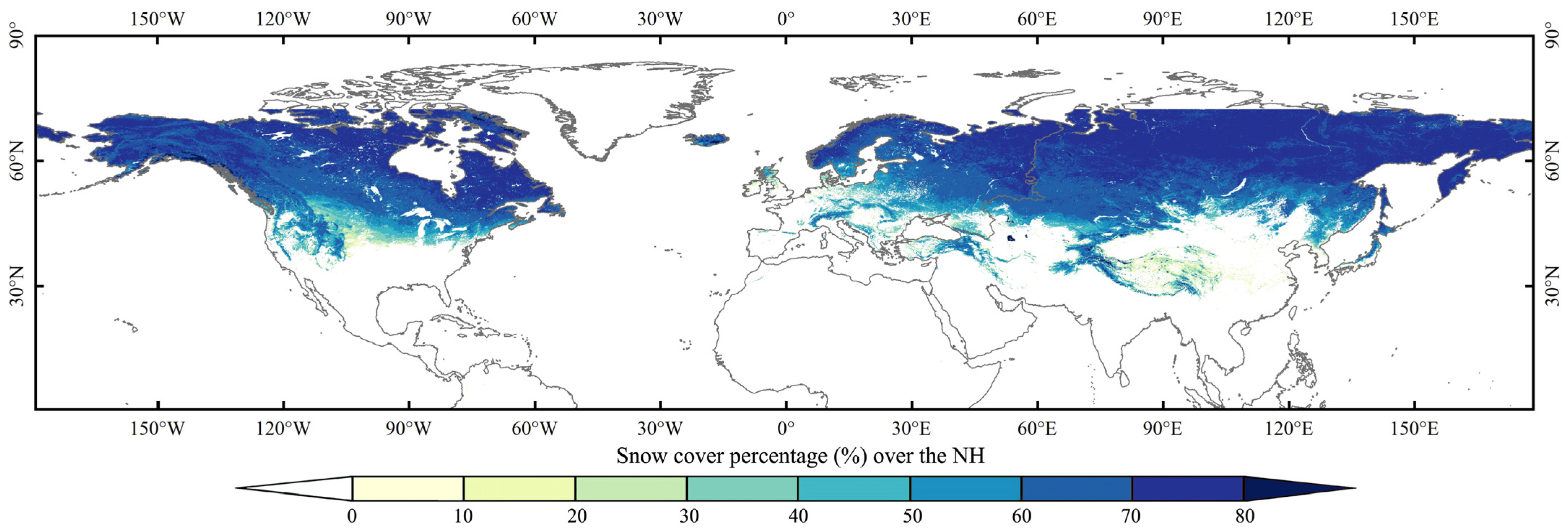
Figure 1. 20-year averaged snow cover percentage (%) in each grid cell across the Northern Hemisphere from 2000 to 2019. January and February 2000 comprised monthly means during 2001–2019.
Remotesensing 13 04938 g001
Figure 2. Three albedo radiative kernels used in this study.
Remotesensing 13 04938 g002
Figure 3. (a) Z-score anomalies of annual mean SCE in the NH, including North America (NA) and Eurasia (EU), during 1972–2019. (b) The seasonal variabilities of SCE in the NH and (c) associated changes in each month during 2000–2019. Blue in (a) represents the period 2000–2019. Changes in (c) were calculated by the monthly mean SCE during 2000–2019 minus the comparable values in the referencing period, 1972–2000.
Remotesensing 13 04938 g003
Figure 4. The 20-year averaged (a) snow cover percentage (%) in March during 2000–2019, and 20-year averaged March surface albedo from (b) C3S ALBH-DH, (c) GLASS, and (d) CLARA-SAL-A2 during 2000–2019. (e) Z-scores of SCE and surface albedo in March during 2000–2019; (f) linear scatter plots between z-scores of SCE and surface albedo in March during 2000–2019. Any missing values were replaced with monthly means from 2000 to 2019.
Remotesensing 13 04938 g004
Figure 5. The 20-year averaged (a) snow cover percentage (%) in June during 2000–2019 and 20-year averaged surface albedo in June from (b) C3S ALBH-DH, (c) GLASS, and (d) CLARA-SAL-A2 during 2000–2019. (e) Z-scores of SCE and surface albedo in June during 2000–2019; (f) linear scatter plots between Z-scores of SCE and surface albedo in June during 2000–2019. Any missing values were replaced with monthly means from 2000 to 2019.
Remotesensing 13 04938 g005
Figure 6. The 20-year (a) annual mean SnRF, (b) changes in annual mean SnRF, (c) interannual variability of annual mean SnRF, (d) intra-annual variability of monthly mean SnRF, and changes in each month during 2000–2019. The error bars in (c,d) are expressed as the range derived from the three SnRF results calculated from different albedo radiative kernels. The solid bars in (d) indicate that the changes in SnRF were statistically significant in a given month during 2000–2019. The hollow bars in (d) indicate that the changes in SnRF were insignificant at the 90% level in a given month during 2000–2019.
Remotesensing 13 04938 g006
Figure 7. CERES observed 20-year annual mean TOA (a) upward shortwave flux, and (b) changes from 2000 to 2019. (c) Interannual variability of the annual mean TOA upward shortwave flux and its linear trend, and (d) linear scatter plots between Z-score anomalies of SnRF and TOA upward shortwave flux over the NH from 2000 to 2019.
Remotesensing 13 04938 g007
Figure 8. (a) Z-score of annual mean SnRF over the NH during 2000–2019 and its relative contribution from each month. (b) The 20-year averaged relative contribution from each month to annual mean SnRF anomalies over the NH from 2000 to 2019.
Remotesensing 13 04938 g008
Table 1. Summary of datasets used in the study.
VariableDatasetHorizontal ResolutionTemporal ResolutionTime SpanPurpose
Snow coverMOD10CM0.05°Monthly2000–2019SCE change detection
NH SCE CDR v01r01Monthly1966–2019
Surface albedoGLASS0.05°8-day2000–2019Albedo contrast calculation
CLARA-SAL-A20.25°5-day2000–2019
C3S-ALBH-DH1-km10-day2000–2019
MCD43GF0.0083°Daily2001–2017
Albedo radiative kernelsCAM32.81°MonthlyRadiative kernel calculation
AM22.50°Monthly
ECHAM61.88°Monthly
TOA shortwave fluxCERES EBAF1.88°Monthly2000–2019Contribution analysis
Publisher’s Note: MDPI stays neutral with regard to jurisdictional claims in published maps and institutional affiliations.