GNSS Imaging of Strain Rate Changes and Vertical Crustal Motions over the Tibetan Plateau

Abstract

In this paper, we perform a comprehensive analysis of contemporary three-dimensional crustal deformations over the Tibetan Plateau. Considering that the coverage of continuous GNSS sites in the Tibetan Plateau is sparse, a newly designed method that mainly contains Spatial Structure Function (SSF) construction and Median Spatial Filtering (MSF) is adopted to conduct GNSS imaging of point-wise velocities, which can well reveal the spatial pattern of vertical crustal motions. The result illustrates that the Himalayan belt bordering Nepal appears significant uplift at the rates of ~3.5 mm/yr, while the low-altitude regions of Nepal and Bhutan near the Tibetan Plateau are undergoing subsidence. The result suggests that the subduction of the Indian plate is the driving force of the uplift and subsidence in the Himalayan belt and its adjacent regions. Similarly, the thrusting of the Tarim Basin is the main factor of the slight uplift and subsidence in the Tianshan Mountains and Tarim Basin, respectively. In addition, we estimate the strain rate changes over the Tibetan Plateau using high-resolution GNSS horizontal velocities. The result indicates that the Himalayan belt and southeastern Tibetan Plateau have accumulated a large amount of strain rate due to the Indian-Eurasian plate collision and blockage of the South China block, respectively.

1. Introduction

The Tibetan Plateau is the largest inland plateau in China (covering an area of about 2.5 million km²) and the highest plateau in the world (the average elevation reaches ~4500 m), which is known as the “roof of the world” and the “third pole” [1,2,3,4]. Due to the Indian–Eurasian plate collision, the Tibetan Plateau is one of the most tectonically active regions in the world, and several large active fault zones are formed inside the Tibetan Plateau [5,6,7]. The tectonic activities of these faults lead to the frequent occurrence of strong earthquakes over the Tibetan Plateau (e.g., 2001 Mw 8.1 Kunlun earthquake, 2010 Mw 7.1 Yushu earthquake, 2013 Ms 7.0 Lushan earthquake, 2015 Mw 7.8 Nepal earthquake, 2020 Mw 6.3 Nima earthquake, and 2021 M 7.4 Maduo earthquake) [8,9,10,11,12,13]. As a continent–continent collision region that is still undergoing strong tectonic deformations, the Tibetan Plateau has become a natural laboratory for understanding plate collisions and geological evolution [14,15,16]. Thus, characterizing a high-resolution crustal deformation field over the Tibetan Plateau has important implications not only for understanding its tectonic motions and dynamic mechanism but also for seismic hazard assessment in mainland China.

Extensive studies associated with the crustal deformations over the Tibetan Plateau and its surrounding regions were carried out with the aid of space geodetic technologies. Gan et al. [17] utilized the observations of ~726 GPS sites to estimate the rigid rotation of the Tibetan Plateau in the Eurasia-fixed reference frame and revealed the deformation features of the interior, southern, northeastern, and eastern parts of the plateau after removing the rigid rotation. Liang et al. [18] established a high-resolution 3D crustal motion field over the Tibetan Plateau using the observations of 750 GPS sites and revealed the tectonic deformation features according to horizontal velocities. Meanwhile, the result also indicated the whole plateau occurs uplift relative to the South China block, while the uplift is insignificant or negative in the surrounding regions. Kreemer et al. [19] established a global GPS horizontal velocity field on basis of 32 studies, which also contains the GPS velocity of the Tibetan Plateau and its surrounding regions. Hao et al. [20] utilized GPS and GRACE to explore the vertical crustal motions of the southeastern Tibetan Plateau, and the focus was on exploring the vertical seasonal variations. Zheng et al. [21] provided the more complete and up-to-date horizontal velocity field of the India–Eurasia collision zone, including 2576 GNSS velocities. Meanwhile, the strain rate change and seismic hazard over this region were evaluated according to the velocity field. Pan et al. [22] explored the spatio–temporal patterns of seasonal oscillations and crustal deformations over the Tibetan Plateau using GPS and GRACE measurements. The results reveal the eastward escape of plastic crustal material in the southeastern Tibetan Plateau and crustal thinning inside the Tibetan Plateau. Wang et al. [23] presented a high-resolution GPS horizontal velocity field of mainland China and its surrounding regions by combining estimated velocities with the velocities published in previous studies and then revealed the tectonic motions and strain rate changes of mainland China.

Whereas, previous studies pay less attention to revealing the spatial patterns of vertical crustal motions over the Tibetan Plateau, which mainly due to the fact that the coverage of continuous GNSS sites is sparse and the vertical component of GNSS observations is susceptible to geophysical factors (e.g., surface mass loading). Liang et al. [18] determined the vertical crustal motions over the Tibetan Plateau based on 165 campaign GNSS sites that only have two phases of observations, which cannot effectively consider the effects of significant seasonal oscillations induced by surface mass loading in the vertical observations. In order to explore the vertical crustal motion over the Tibetan Plateau based on the sparse continuous GNSS sites, a newly designed GNSS imaging method is adopted to carry out imaging for the point-wise velocities, and then reveal the features of vertical crustal motions in a continuous space. In addition, we also estimate the surface mass changes over the Tibetan Plateau using Gravity Recovery and Climate Experiment (GRACE) mascon solutions in order to better explore the spatial patterns of vertical crustal motions. Meanwhile, we also construct an up-to-date GNSS horizontal velocity field by combining with the latest studies and revealing the tectonic motions and strain rate changes over the Tibetan Plateau. According to the spatial distribution of GNSS velocities and strain rate changes, the tectonic activity and seismic hazard over the Tibetan Plateau are assessed.

2. Datasets and Methods

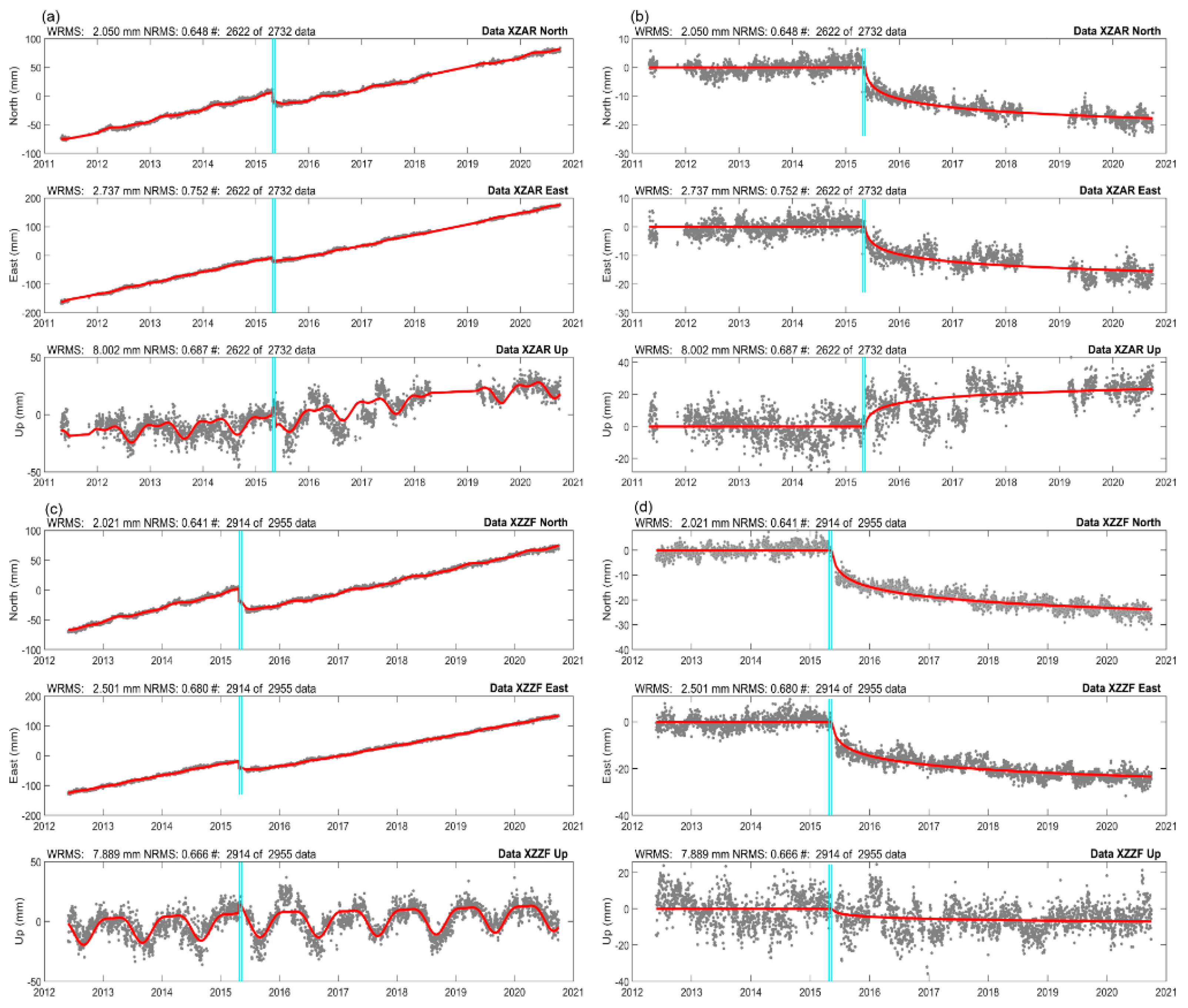
2.1. GNSS Datasets

In order to explore the properties of crustal motions over the Tibetan Plateau, 153 continuous GNSS sites derived from Crustal Movement Observation Network of China (CMONOC) are selected (Figure 1). The position time series of GNSS sites are provided by the GNSS data product service platform of China Earthquake Administration (ftp://ftp.cgps.ac.cn/products/position/, accessed on 15 October 2021), and GAMIT/GLOBK 10.4 is utilized to carry out GNSS data processing [24]. The unconstrained daily solutions for satellite orbits and positions of GNSS sites are obtained by GAMIT, and then aligned to the ITRF reference frame using GLOBK. More details about the GNSS data processing can refer to ftp://ftp.cgps.ac.cn/doc/processing_manual.pdf, accessed on 15 October 2021.

Meanwhile, we also adopt the position time series of 52 continuous GNSS sites located in Nepal and Bhutan near the Tibetan Plateau (Figure 1), which is available at the Nevada Geodetic Laboratory (NGL) (http://geodesy.unr.edu/, accessed on 15 October 2021). The time span of all GNSS position time series ends to 2020.7500. The GNSS data processing is conducted by GIPSY-OASIS-II software. NGL analysis center utilizes ionospheric independent combination to remove ionospheric effects, Global Mapping Function (GMF) model to correct tropospheric delays, FES 2004 to correct tidal loading effects, and antenna phase center correction parameters refer to the absolute antenna phase calibration file provided by the International GNSS Service (IGS) center.

Due to the impact of several strong earthquakes, some sites have recorded significant coseismic and postseismic deformations. Considering this problem, we model the position time series of continuous GNSS sites according to the modeling scheme described in Xiang et al. [25], which can simultaneously extract and model the linear, annual, semi-annual, coseismic, and postseismic signals [26,27,28]. Figure 2 displays the modeled signals of GNSS position time series for sites XZAR and XZZF. In addition to these continuous GNSS sites, we also collect some horizontal velocities published in recent studies, which mainly contain the GNSS horizontal velocities published in Kreemer et al. [19] and Wang et al. [23]. The rigid body rotation is utilized to convert these published velocities to coincide with our solutions, and all GNSS horizontal velocities are relative to the Eurasian plate [29].

2.2. GRACE Datasets

The Gravity Recovery and Climate Experiment (GRACE) and GRACE Follow-On (GFO) are dual-satellite missions monitoring and mapping Earth’s changing gravity field. GRACE produced monthly gravity field solutions from April 2002 to June 2017, and GFO continues this record starting in June 2018. Compared with Spherical Harmonic (SH) solutions, mascon solutions can be applied from the regional to global scales. In addition, mascon solutions do not require de-striping and signal restoration, which also have a higher signal-to-noise ratio [30].

In order to estimate the trend and annual amplitude induced by surface mass changes over the Tibetan Plateau, the Goddard Space Flight Center (GSFC) mascon solutions provided by GeoForschungs Zentrum (GFZ) Potsdam are adopted in this paper (https://earth.gsfc.nasa.gov/geo/data/grace-mascons, accessed on 15 October 2021). The GSFC mascon solution consists of 41,168 equal-area, 1 arc-degree mascon cells. GGM05C is chosen as the static gravity field model in the solution, the GOT4.7 model of order 90 is adopted as the tidal model, and the RL06 Atmosphere and Ocean De-aliasing Level-1B (AOD1B) product is regarded as the atmospheric and oceanic de-aliasing model [31]. Meanwhile, the Jet Propulsion Laboratory (JPL) TN-13 is utilized to conduct the Geocenter corrections, the TN-14 is utilized to replace the original C20 terms, and the ICE-6G_D is used to correct the Glacial Isostatic Adjustment (GIA) effects. In general, surface mass changes estimated by GRACE/GFO can be expressed as Equivalent Water Height (EWH).

2.3. Strain Rates Estimation

In this paper, the vel2strain code developed by the Institute of Seismology, China Earthquake Administration is utilized to estimate the strain rate changes in the Tibetan Plateau. The vel2strain code is written in Fortran, which mainly adopts the method described in Shen et al. [32] and Shen et al. [33]. Shen et al. [32] proposed an algorithm that utilizes an improved least squares method to model strain as a continuous function, which iterates over a two-dimensional space with arbitrarily small increments to ensure the continuity of solution. The horizontal velocity field is expanded to its first derivative at each interpolation position R, which is represented by a rigid block motion (translation and rotation) model and a uniform strain field. The displacement can be expressed by the following formula.

$$d=Am+\epsilon$$

(1)

where A is the partial derivative matrix, d is the data vector, $\epsilon$ is the error vector. Among them, m denotes the vector of strain, translation, and rotation, which can be expressed by the following formula in the case of horizontal strain.

$$m={(U_x,U_y,\omega ,{\tau }_{xx},{\tau }_{xy},{\tau }_{yy})}^T$$

(2)

where $U_x$ and $U_y$ are the translation components in the x and y components, ${\tau }_{xx}$, ${\tau }_{xy}$, and ${\tau }_{yy}$ are the horizontal strain components, and $\omega$ is rotation. The Formula (1) can also be expressed as:

$$\left[\begin{array}{l}{V}_{x1}\\ V_{y1}\\ V_{x2}\\ V_{y2}\\ \dots \\ V_{xn}\\ V_{yn}\end{array}\right]=\left[\begin{array}{l}1,0,{\Delta }_{y1},{\Delta }_{x1},{\Delta }_{y1},0\\ 0,1,-{\Delta }_{x1},0,{\Delta }_{x1},{\Delta }_{y1}\\ 1,0,{\Delta }_{y2},{\Delta }_{x2},{\Delta }_{y2},0\\ 0,1,-{\Delta }_{x2},0,{\Delta }_{x2},{\Delta }_{y2}\\ \dots \\ 1,0,{\Delta }_{yn},{\Delta }_{xn},{\Delta }_{yn},0\\ 0,1,-{\Delta }_{xn},0,{\Delta }_{xn},{\Delta }_{yn}\end{array}\right]\left[\begin{array}{l}{U}_x\\ U_y\\ \omega \\ {\tau }_x\\ {\tau }_{xy}\\ {\tau }_y\end{array}\right]+\left[\begin{array}{l}{\epsilon }_{x1}\\ {\epsilon }_{y1}\\ {\epsilon }_{x2}\\ {\epsilon }_{y2}\\ \dots \\ {\epsilon }_{xn}\\ {\epsilon }_{yn}\end{array}\right]$$

(3)

where $V_{xi}$ and $V_{yi}$ denote the displacement components of the i-th site located at $r_i$, ${\Delta }_{xi}$ and ${\Delta }_{yi}$ denote the components of $\Delta R_i=r_i-R$. Assuming that C is the covariance matrix of velocities, we can obtain a least-square solution:

$$m={(A^T{C}^{-1}A)}^{-1}{A}^T{C}^{-1}d$$

(4)

However, the above solution is the average strain field of the whole region. In order to give more weight to the sites closer to site R, a uniform Gaussian spatial weighting function ($G_i=L_i\ast Z_i$) is adopted. $L_i$ and $Z_i$ are functions that depend on distance and space coverage. The distance-dependent weighting $L_i$ can be defined as:

$$L_i=\exp (-\raisebox{1ex}{$\Delta R_i^2$}\!\left/ \!\raisebox{-1ex}{$D^2$}\right.)$$

(5)

where D is the spatial smoothing parameter. The larger D (i.e., the greater the weight of far-field velocities), the higher the smoothness of strain rate field and the smaller the surface error of strain rate estimation.

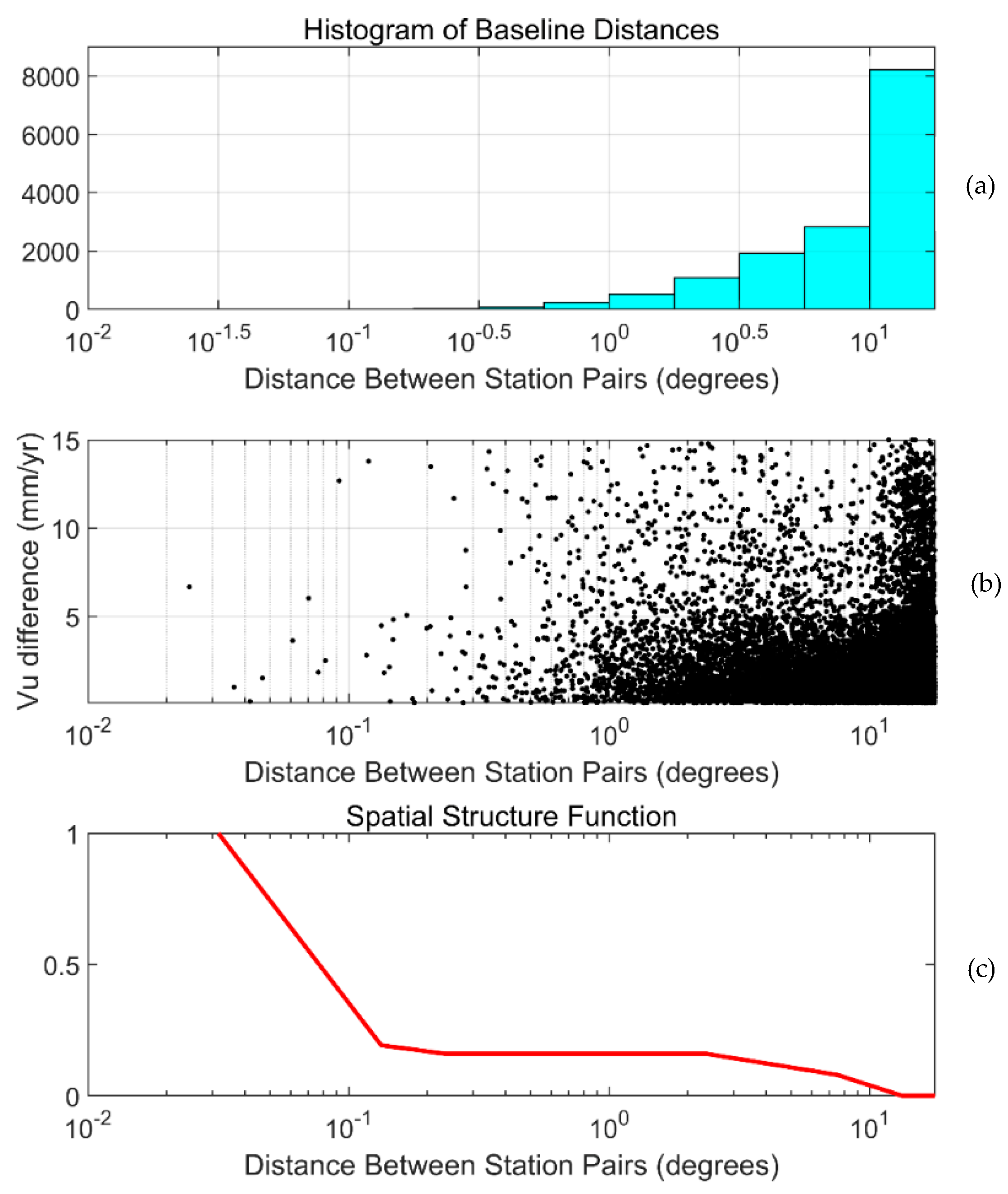
2.4. GNSS Imaging Scheme

GNSS imaging method is a newly designed method that can generate the image of vertical crustal motions based on point-wise GNSS velocities, which can effectively describe the spatial patterns of vertical crustal motions in continuous space [34,35,36,37,38]. The Spatial Structure Function (SSF) is utilized to describe the correlation between the velocities of GNSS sites, and then the filtering that considers spatial structure is constructed to eliminate outliers and enhance the regional common signals. After that, the velocity field is encrypted according to the image processing technology, and then realize the spatial–temporal features extraction of vertical crustal motions. In this paper, we briefly introduce the GNSS imaging scheme, which mainly contains the construction of SSF and Median Spatial Filtering (MSF) based on SSF.

(1)

Spatial structure function

SSF groups the GNSS site pairs based on the distances between sites, and builds the mapping relationship between the distances and velocity correlation based on the statistical results of velocity differences, which can reflect the correlation of different GNSS velocities. Firstly, we calculate the absolute value of velocity difference $\delta v_{ij}$ ($i=1,2,\dots ,n;j=1,2,\dots ,n$) and corresponding distance ${\Delta }_{ij}$ of each site pair, and sort them according to the distance of site pair. The central angle of large arc formed by site pair is regarded as the distance of site pair, and the absolute value of velocity difference is calculated by:

$$\delta v_{ij}=\left|v_i-v_j\right|$$

(6)

where $v_i$ and $v_j$ are the velocity of $i$-th and $j$-th sites.

Secondly, several data pools are divided based on the distance of site pair. In general, $0.25lo{g}_{10}\Delta$ is regarded as the separation distance of data pools to ensure that each data pool contains at least 20 site pairs. The MAD of the absolute value of GNSS velocity difference in each data pool is calculated.

$$MA{D}_k=median\left|\delta v_i-\delta \widehat{v}\right|(i=1,2,\dots ,n;k=1,2,\dots ,m)$$

(7)

Among them, $MA{D}_k$ is the MAD of $k$-th data pool, $\delta v_i$ is the absolute value of $n$ velocity difference in each data pool, and $\delta \widehat{v}$ is the median of velocity difference in all data pool.

Finally, we can construct and standardize the SSF according to the following formula:

$$ss{f}_i=\{\begin{array}{l}\frac{1}{\max (MA{D}_i,MA{D}_{i+1})}(i=1,2,\dots ,m-1)\\ \frac{1}{MA{D}_i}(i=1,2,\dots ,m)\end{array}$$

(8)

$$ss{f}_i=\frac{ss{f}_i}{\max (ss{f}_1,\dots ,ss{f}_m)}(i=1,2,\dots ,m)$$

(9)

where $ss{f}_i$ is the SSF value of $i$-th data pool, and $MA{D}_i$ is the MAD of $i$-th data pool.

(2)

Median spatial filtering

In this paper, the velocity value of each site is screened by MSF taking into account the spatial structure, which can enhance the commonality of vertical velocities. Firstly, the spherical Delaunay triangulation is utilized to build the spatial relationship between different sites. Then, one GNSS site is selected as the filtering site. The velocity uncertainty and spatial correlation are simultaneously estimated, and the weights of sites connected to the filtering site in the triangulation network are calculated and standardized.

$${\omega }_i=\frac{ss{f}_i}{{\sigma }_i}$$

(10)

$${\omega }_i^{\prime }=\frac{{\omega }_i}{{\displaystyle \sum _{i=1}^n{\omega }_i}}$$

(11)

where $ss{f}_i$ is the spatial structure function value obtained by inputting the distance between the current site and estimated site, ${\sigma }_i$ is the velocity uncertainty of each site, ${\omega }_i$ and ${\omega }_i^{\prime }$ denote the weights before and after standardization.

In order to encrypt the discrete GNSS network, the research region is divided into grid, and each grid point is regarded as a filtering site. According to the velocities and uncertainties of surrounding sites, MSF interpolation is utilized to obtain the velocity of each grid point, and then the GNSS image of vertical crustal motions is generated. Compared with other methods, GNSS imaging can effectively eliminate the impact of outliers in velocities, which can accurately describe common features of vertical crustal motions.

3. Results

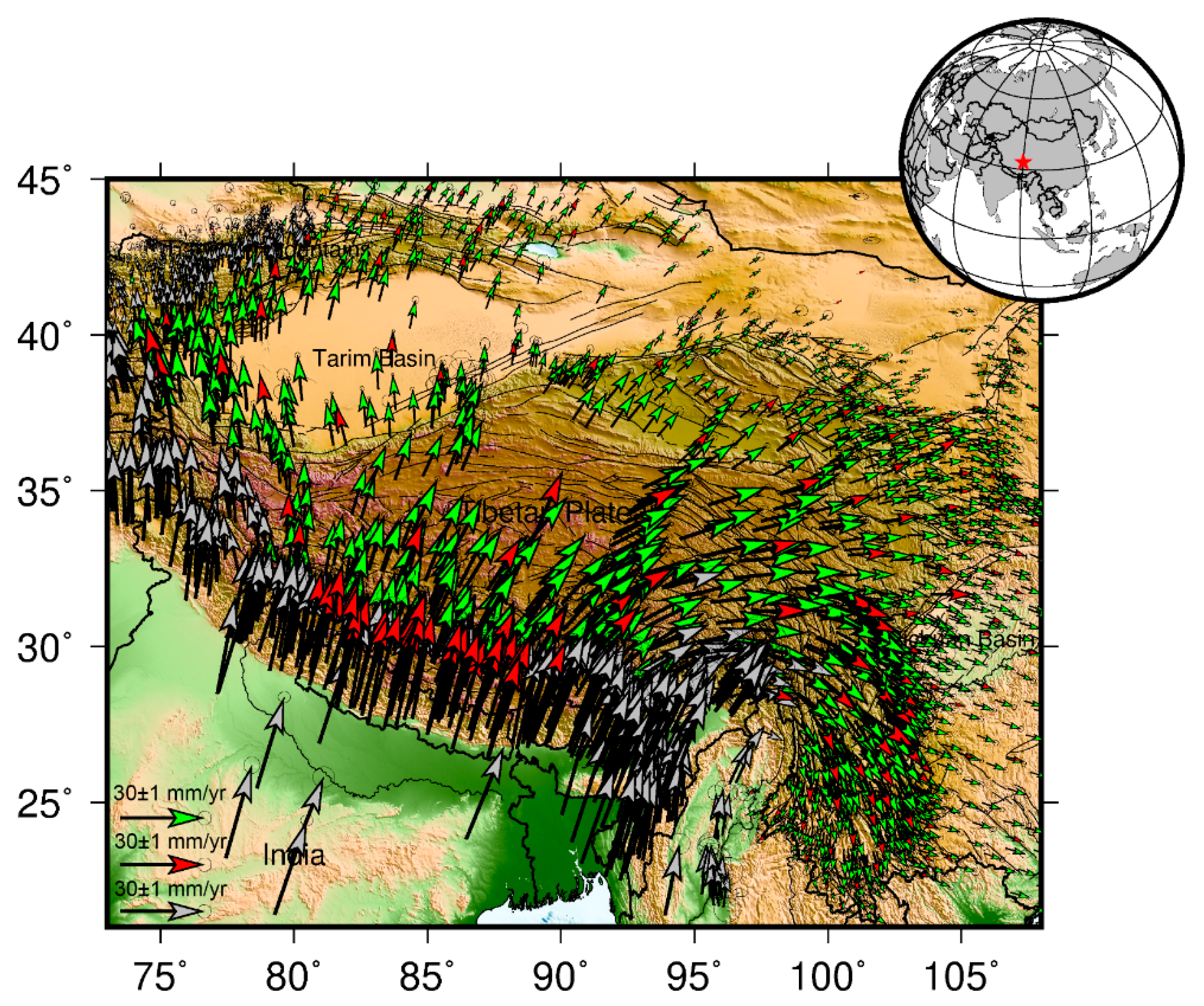
3.1. GNSS Horizontal Velocity Field

By combining with previous studies, a high-resolution GNSS horizontal velocity field over the Tibetan Plateau and its surrounding regions is established (Figure 3), which contains 2032 GNSS velocities. The GNSS velocity field clearly describes the crustal motions over the Tibetan Plateau. The Indian plate is pushing the Eurasian plate in the NE direction, and the velocities decrease sharply along the NE direction. Meanwhile, the motions of the Tibetan Plateau are blocked by the South China block, resulting in the significant clockwise rotation of the GNSS velocity field in the southeastern Tibetan Plateau. In addition, the GNSS velocity field also appears weak clockwise rotation in the Tarim Basin due to the thrusting of the Tarim Basin. The spatial patterns of the GNSS velocity field reveal the obvious lateral extrusion in the Tibetan Plateau, which is consistent with the conclusions of previous studies [18,21,23].

Meanwhile, we also display the spatial distribution of the GNSS velocity field in the EW and NS directions, and the statistical results of velocities and uncertainties (Figure 4). Most GNSS velocity uncertainties are less than 1 mm/yr, indicating that the estimated GNSS velocity field is reliable. The rate of GNSS velocity ranges from −8.4 to 25.6 mm/yr in the EW direction, and it varies from −15.1 to 39.4 mm/yr in the NS direction. For the east component of GNSS velocity, the large rates are concentrated in the southeastern Tibetan Plateau, which coincides with the clockwise rotation of the GNSS velocity field in this region. As for the north component of the GNSS velocity, the rates are obviously reduced along the NE direction, suggesting that the Tibetan Plateau and its surroundings have produced significant crustal shortening along the NE direction due to the collision of the Indian and Eurasian plates.

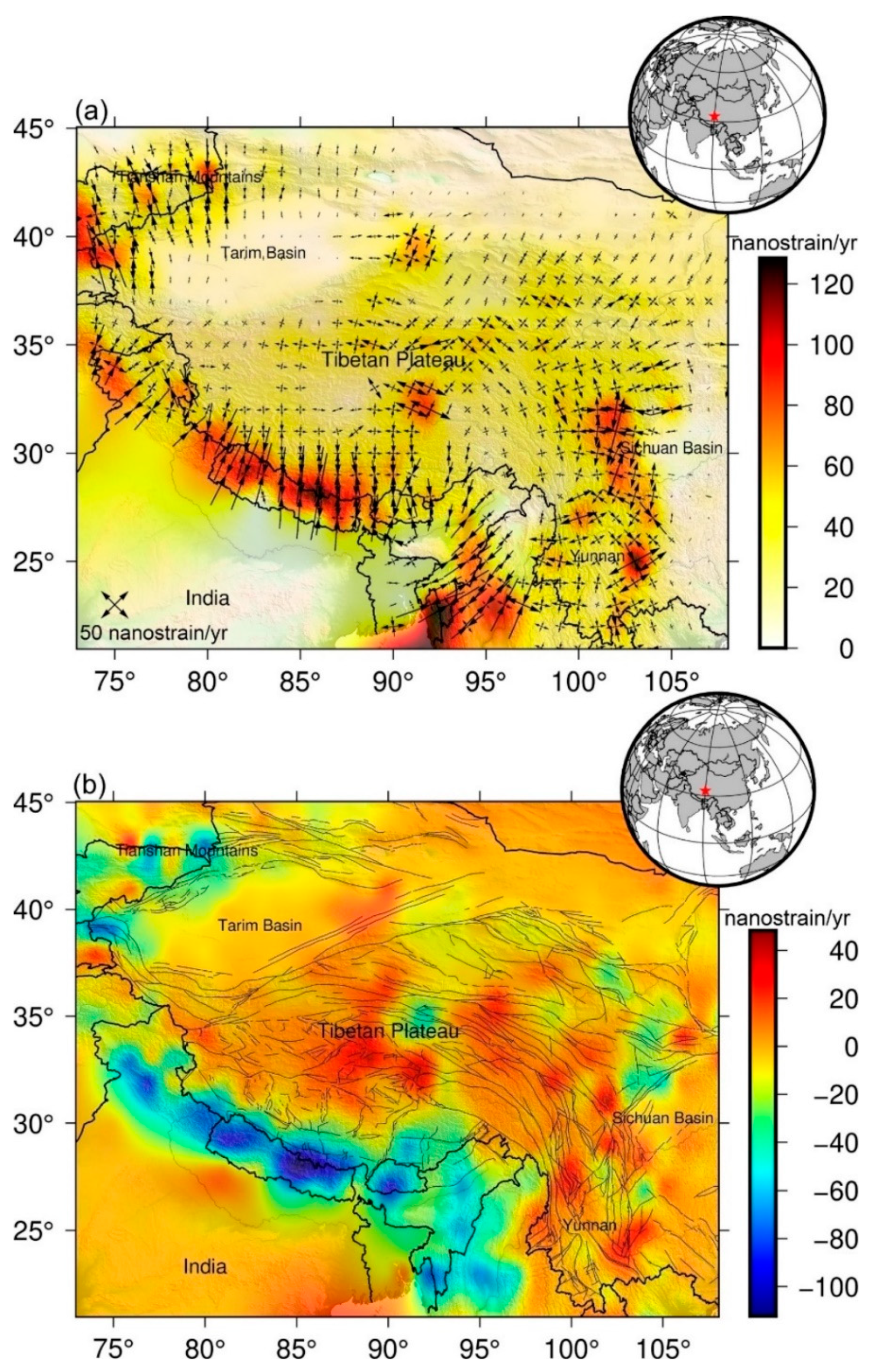
3.2. Strain Rate Changes

In order to explore the tectonic activities over the Tibetan Plateau, the strain rate changes in this region are characterized based on the high-resolution GNSS velocity field. The region is divided into a grid by 1° of latitude and longitude, and the strain rate of each grid point is estimated by the method described in Section 2.4.

As depicted in Figure 5a, a large amplitude of principal strain rate is accumulated in the Himalaya arc tectonic belt, including Nepal, Bhutan, northwestern and northeastern India, which is dominated by the extrusion strain rate. The Himalaya tectonic belt is the foreland of the Indian–Eurasian plate collision, and rapid plate convergence leads to significant strain rate accumulation. The principal strain rate in the southeastern Tibetan Plateau is also dominated by the extrusion strain rate, mainly because the motion of the Tibetan Plateau is blocked by the South China block. In addition, the principal strain rate in the Tianshan belt is mainly manifested as extrusion strain rate, implying that the thrusting of Tarim Basin has induced the extrusion deformations in the Tianshan belt to a certain extent. The amplitude of principal strain rate in the Sichuan Basin and Tarim Basin is relatively small (within 10 nanostrain/yr (i.e., ${10}^{-8}$/yr)), indicating that these regions are relatively stable without too much strain rate accumulation.

For the maximum shear strain rate, the large value is accumulated in four regions (i.e., Himalaya arc tectonic belt, eastern Tibetan Plateau, Tianshan Mountains, and some regions of Myanmar and Bangladesh) (see the background color in Figure 4a). The peak of maximum shear strain rate is located at the Himalayan tectonic belt, and the maximum reaches 128.5 nanostrain/yr. The second is the eastern Tibetan Plateau and some regions of Myanmar and Bangladesh, and the maximum shear strain rate values are all above 80 nanostrain/yr. The maximum shear strain rate inside the Sichuan Basin and Tarim Basin is close to 0 nanostain/yr, which also suggests that the interior of the Sichuan Basin and Tarim Basin is relatively stable.

The dilatational strain rate over the Tibetan Plateau varies from −112.3 to 48.2 nanostrain/yr with the mean of −10.5 nanostrain/yr (Figure 5b). Similarly, the large-scale negative dilatational strain rate is focused on the Himalayan arc tectonic belt, suggesting that this region has undergone crustal extrusion deformation. Meanwhile, some small-scale negative dilatational strain rate appears in the Tianshan belt and eastern Tibetan Plateau. The dilatational strain rates inside the Tibetan Plateau at the longitude of 87° to 95° are positive, implying that the crust inside the Tibetan Plateau has experienced extension deformation. The junction of Tibetan Plateau and South China block (e.g., some regions of Yunnan and Sichuan provinces) also occurs large-scale positive dilatational strain rate, which can be attributed to the extrusion deformation induced by the blockage of South China block.

The above results demonstrate that the Himalayan orogenic belt has accumulated a large amount of strain rate due to the collision of the Indian plate and Eurasian plate, and the tectonic motions of the entire Himalayan arc belt are quite active, which still belongs to the region with seismic hazard risk. In addition, since the motions of the Tibetan Plateau are blocked by the South China block, a large amount of strain rate has also accumulated at the junction, which is also one of the tectonically active regions in mainland China.

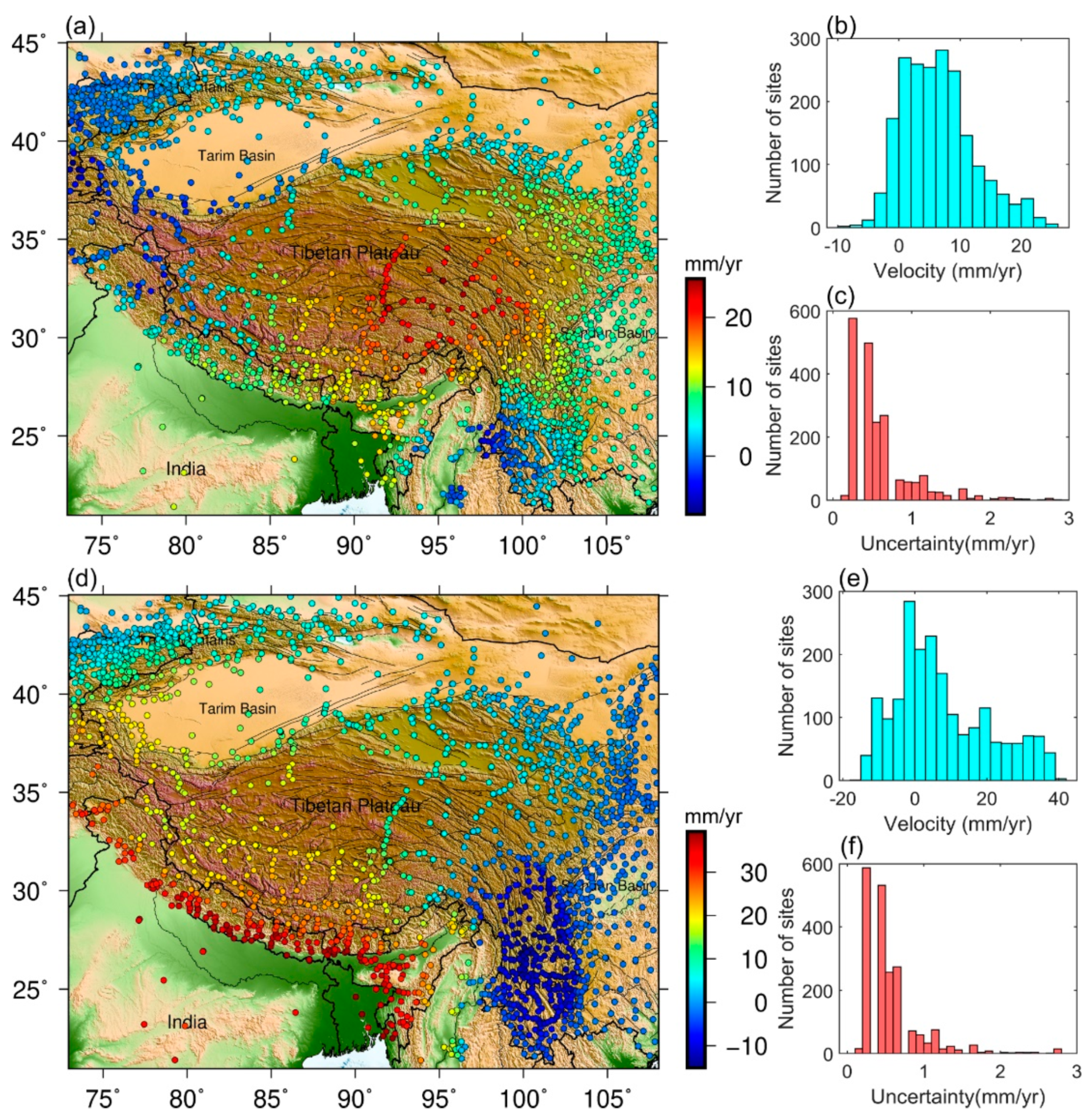
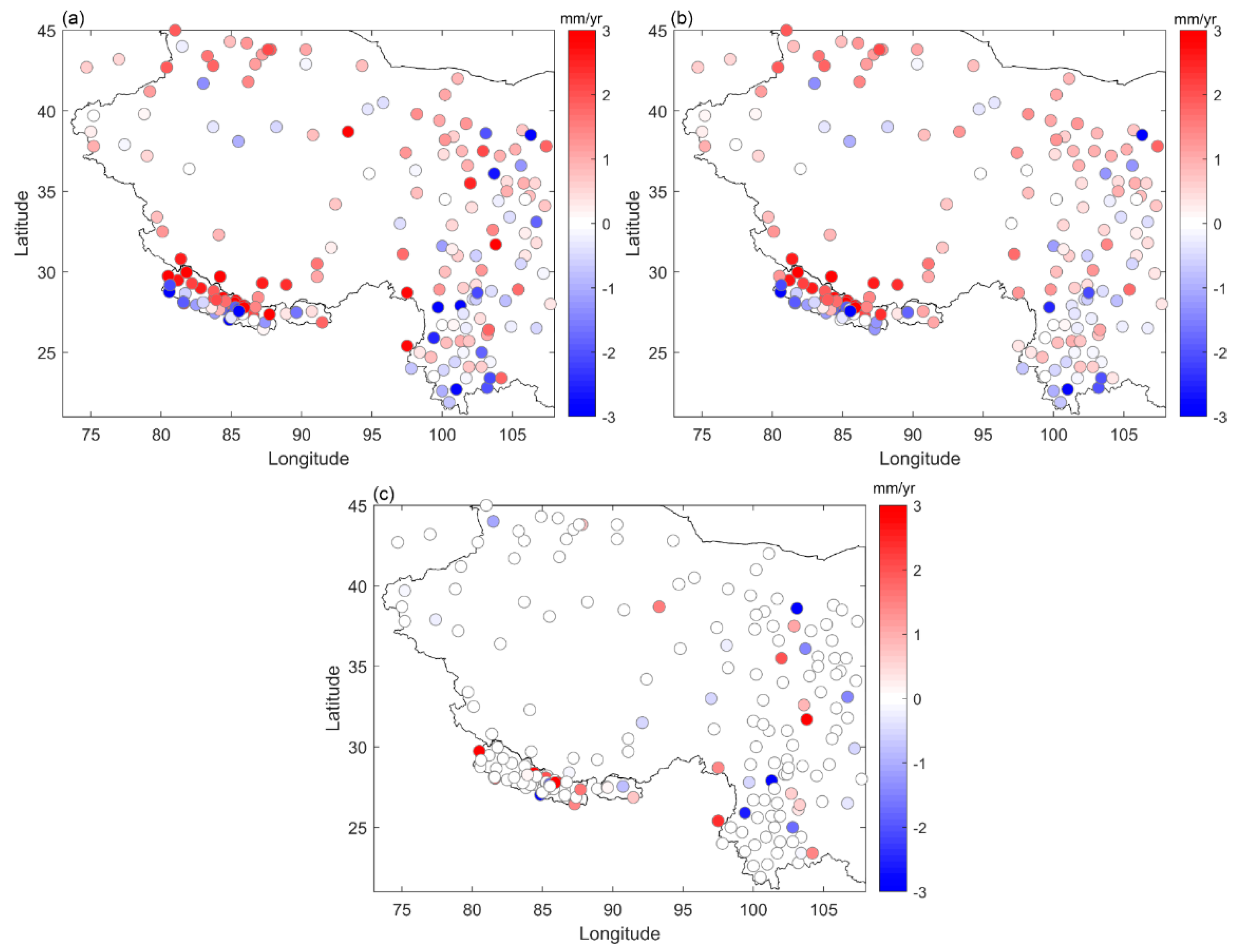
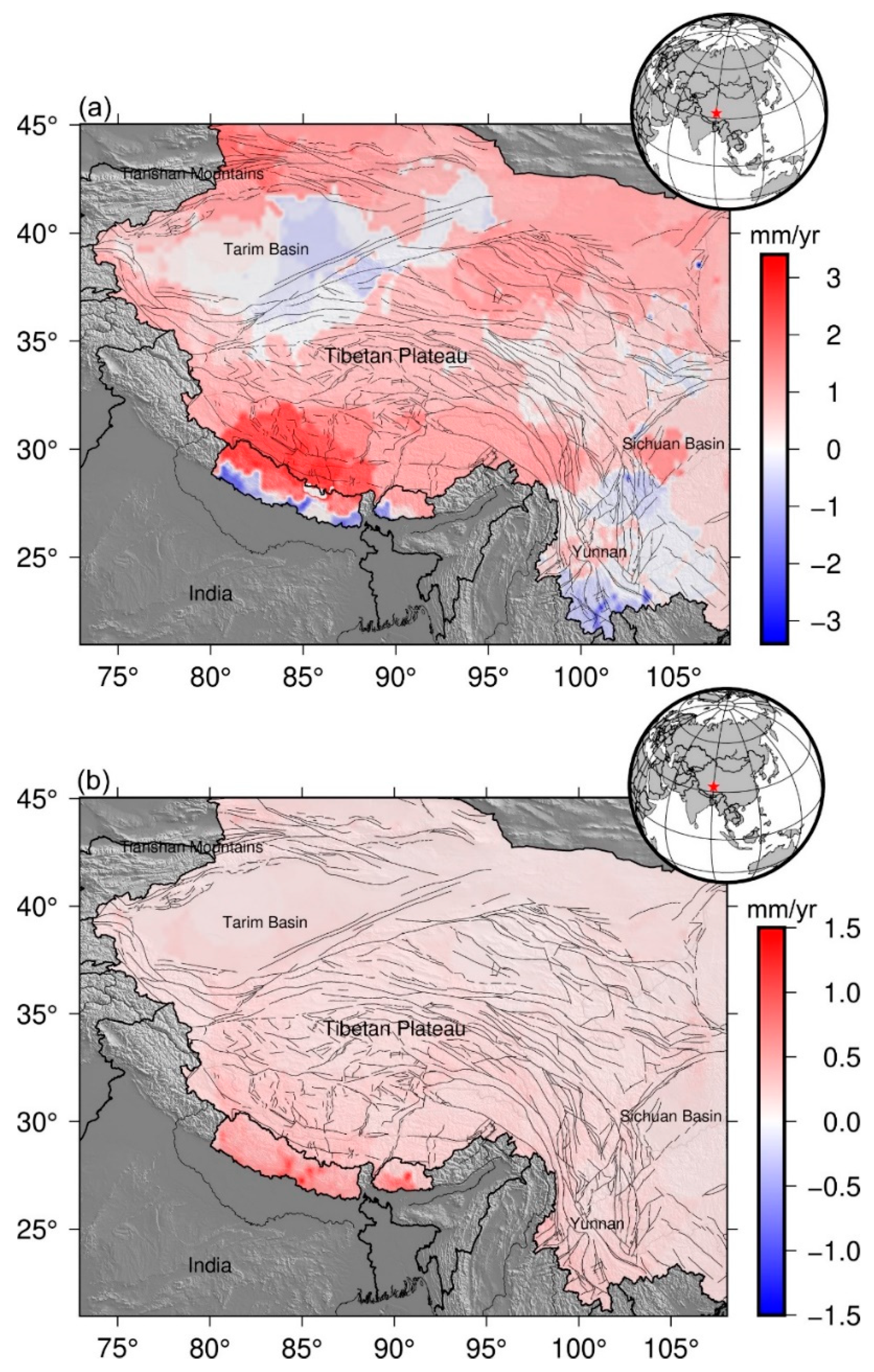
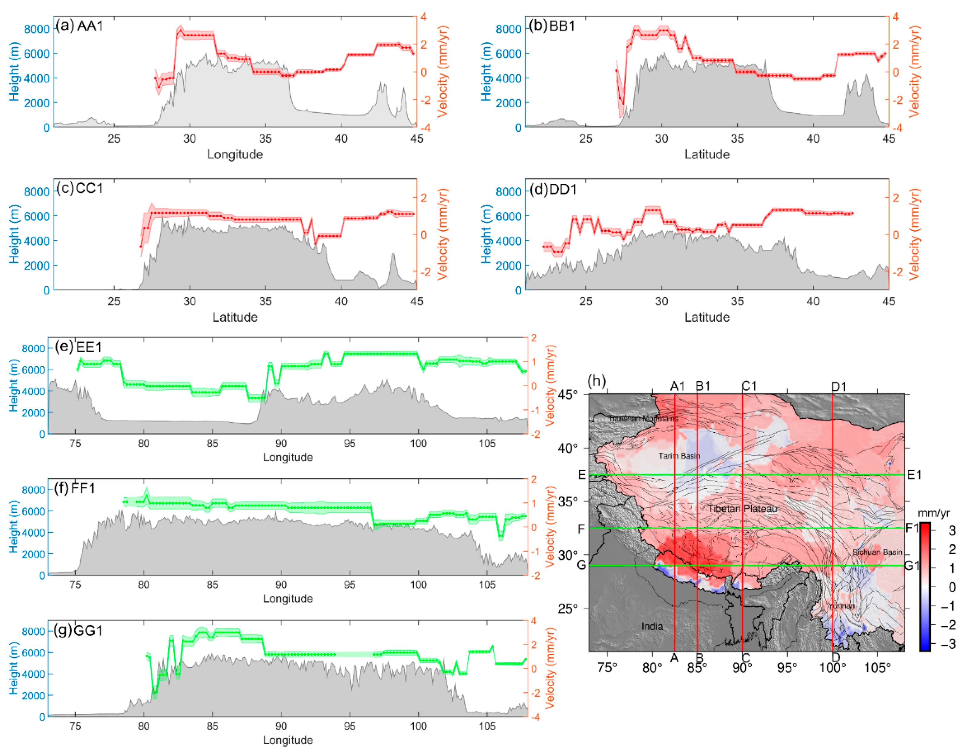
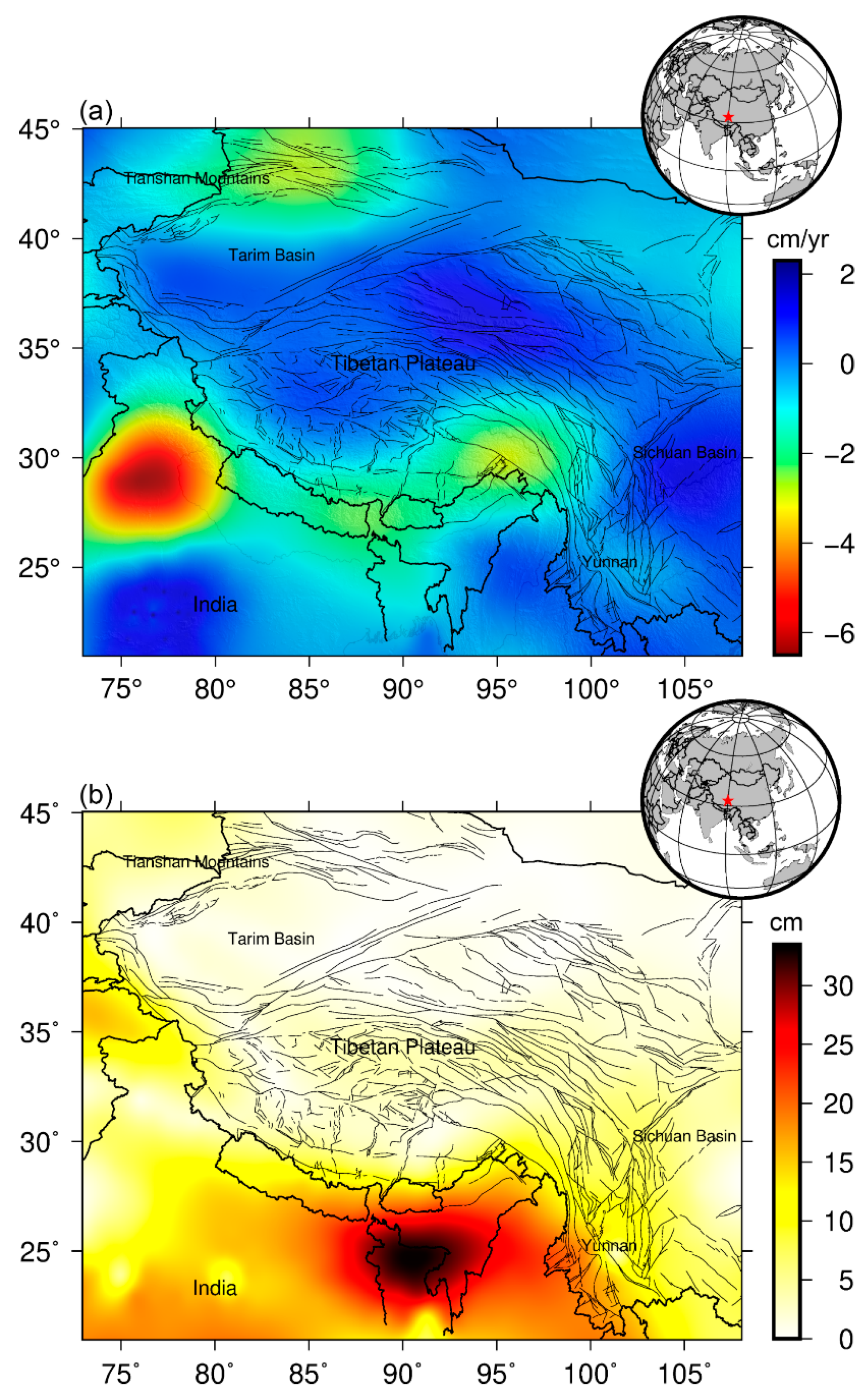
3.3. GNSS Imaging of Vertical Crustal Motions

Up to now, few studies have released the GNSS vertical velocity field of the Tibetan Plateau, and most of them explore the vertical crustal motion over the Tibetan Plateau based on sparse continuous GNSS sites, which have relatively abundant observations. Liang et al. [18] had released the GNSS vertical velocity field of the Tibetan Plateau on basis of dense campaign GNSS sites. However, only two phases of campaign GNSS observations are utilized to estimate the vertical velocity, which cannot consider the effects of significant seasonal oscillations induced by surface mass loading. Thus, we adopt the GNSS imaging method to generate an image of vertical velocity based on the discrete-continuous GNSS network and then reveal the spatial patterns of vertical crustal motions over the Tibetan Plateau.

Firstly, we construct the Spatial Structure Function (SSF) to contain information representing the vertical signal variance, which can be attributed to the distance (i.e., $\Delta$) between GNSS sites. In general, GNSS sites close to each other will exhibit more similar crustal motion features. For each pair of GNSS sites, the absolute value of vertical velocity difference is calculated, and Figure 6b presents the distribution of differences along $lo{g}_{10}(\Delta )$. According to Formulas (8) and (9), the SSF is constructed and normalized, and the value of SSF as a function of distance is depicted in Figure 6c. The value of SSF decreases monotonically as the distance between GNSS sites increases, and it reaches 0 when the distance between sites is around 13.34 km.

Secondly, the Median Spatial Filtering (MSF) is adopted to perform spatial filtering for GNSS vertical velocities, which can reduce the effect of outliers that are obviously different from neighboring velocity rates. MSF utilizes the spherical Delaunay triangulation to connect the evaluation point (i.e., one GNSS site that the spatial filtering is performed) and its nearest neighboring sites, and the weighted median of neighboring velocity rates are computed according to Formulas (10) and (11). Then, the weighted median of the velocities of neighboring sites can be regarded as the velocity rate of the evaluation point. MSF can reduce the importance of sites with large uncertainty and increase the importance of sites near the evaluation point. Figure 7a,b present the original and filtered GNSS vertical velocities in the Tibetan Plateau, and the differences of original and filtered velocities are depicted in Figure 7c. This result indicates that the outliers in the original GNSS velocities are effectively removed, and thus highlighting the common crustal motion signal supported by multiple sites.

Finally, we carry out GNSS imaging of point-wise velocities to generate an image of vertical crustal motions over the Tibetan Plateau. This region is divided into a grid by 0.5° of latitude and longitude. Similarly, we establish the spatial structure relationship between each grid point and neighboring sites using spherical Delaunay triangulation. The velocity of each grid point can be replaced by the weighted median of the velocities of neighboring sites. Figure 8a,c display the GNSS imaging of vertical crustal motions using the filtered velocities and velocities without median spatial filtering applied, respectively. Figure 8e presents the GNSS imaging of vertical crustal motion using the filtered velocities, while each grid is replaced by the weight mean of the velocities of neighboring sites. Compared with the image generated by the filtered GPS velocities, the image of vertical crustal motions generated by the unfiltered velocities is more susceptible to the outliers of velocity rate. Meanwhile, if each grid is replaced by the weighted mean of the velocities of neighboring sites, the estimated image of vertical crustal motions tends to be rough and unreliable.

As described in Figure 9, the spatial patterns of vertical crustal motions over the Tibetan Plateau are diverse, which may be associated with the complex geological, topographical, hydrological, and climate features of the Tibetan Plateau. The large-scale crustal uplift is focused on the southern Tibetan Plateau, especially for the Himalaya belt bordering Nepal, where the uplift rates are about 3.5 mm/yr. However, some regions of Nepal and Bhutan near the Tibetan Plateau experience remarkable crustal subsidence as altitude decreases, suggesting that the significant crustal subduction appears under the Himalayas. Apart from these regions, there are slight crustal uplifts in the Tianshan belt and northern Tibetan Plateau, and the Tarim Basin occurs slight subsidence. In addition, southwest China (i.e., some regions of Yunan and Sichuan provinces) weak crustal subsidence with rates of 0 to 1 mm/yr also appear, which may be related to the gain of hydrological mass induced by the slight increase in annual mean precipitation.

Moreover, we extract seven profiles throughout the Tibetan Plateau along AA1, BB1, CC1, DD1, EE1, FF1, and GG1 (Figure 10) in order to better reveal regional vertical crustal motions. The first three profiles along AA1, BB1, and CC1 clearly exhibit the vertical crustal motions across the southern Himalayas. The vertical crustal motions are dominated by subsidence at the low-altitude regions of Nepal and Bhutan outside the Tibetan Plateau, and rapid crustal uplift with the rates of 1–5 mm/yr is found in the Himalaya belt beyond the subduction of the Indian plate. As latitude increases, the vertical crustal motions are followed by subsidence in the Tarim Basin and slight uplift in the Tianshan Mountains. The three profiles along EE1, FF1, and GG1 pass through the Tibetan Plateau and its surrounding regions at the latitude of 37.5°, 32.5°, and 29°. Similarly, slight subsidence occurs in the Tarim Basin and southwest China in comparison with the Tibetan Plateau.

3.4. Surface Mass Changes over the Tibetan Plateau

In addition to the seasonal oscillations induced by surface mass loading, the long-term gain and loss of surface mass can also result in the crustal uplift and subsidence [39,40,41,42]. Thus, aiming to better explore the properties of vertical crustal motions over the Tibetan Plateau, we also determine the trends and annual amplitudes of surface mass changes based on GRACE mascon solutions. The values of surface mass change trends over the Tibetan Plateau range from −6.42 to 2.25 cm/yr, and the annual amplitudes of surface mass changes vary from 0 to 33.2 cm/yr. As depicted in Figure 11, three regions that exhibit negative surface mass changes are northwest India, the Himalayas, and Tianshan. Among them, the anomalous surface mass loss in northwest India may be associated with the water resource changes induced by groundwater over-exploitation, and the surface mass loss in the Himalayas and Tianshan is mainly attributed to the glacier ice melting.

The surface mass changes over the northern and central Tibetan Plateau, Tarim Basin, and southwest China (e.g., Yunan and Sichuan provinces) occur large-scale positive trends. One potential reason for the positive trends is the gain of hydrological mass induced by the slight increase in annual mean precipitation in these regions. Unlike the surface mass change trends, the large values of the annual amplitudes of surface mass changes are mainly concentrated in low-latitude coastal regions and gradually decrease as the latitude increases. In general, the annual amplitude can reveal the effects of surface mass loading, and this result suggests that the effects of surface mass loading in coastal regions are obviously stronger than in other regions. Combined with the image of vertical crustal motions, it can be found that the surface mass changes can only partly explain the vertical crustal motions of the Tibetan Plateau. Thus, for most regions of the Tibetan Plateau, the tectonic motions, surface mass changes, and other geophysical factors jointly lead to the crustal uplift and subsidence.

4. Discussion

4.1. Tectonic Process of Tibetan Plateau

In this paper, we construct a high-resolution GNSS horizontal velocity field by combining our results and the latest studies, which clearly describe the spatial patterns of crustal motions over the Tibetan Plateau and its surroundings. Meanwhile, we also display the spatial distribution of the east and north components of GNSS horizontal velocities, and it can reveal the changes of horizontal crustal motions more intuitively.

It can be found the Indian plate is pushing the Eurasian plate in the NE direction, and the velocities decrease sharply from 40 to 10 mm/yr along the NE direction, revealing the continuous crustal shortening over the Tibetan Plateau due to the pushing of the Indian plate. In the interior of the Tibetan Plateau, GNSS horizontal velocity starts to “escape” laterally along the east and west directions. Due to the blockage of the South China block, the southeastern Tibetan Plateau occurs in an obvious clockwise rotation. The Tarim Basim displays weak clockwise rotation, and the Tianshan belt also appears crustal shortening due to the thrusting of the Tarim Basin. Many studies have made efforts to reveal the patterns of crustal motions over the Tibetan Plateau [8,17,18,21], and our results are consistent with previous studies.

Based on the GNSS velocity field, the strain rate changes over the Tibetan Plateau and its surrounding regions are estimated. In total, four regions that have accumulated a large amount of strain rate are the Himalaya arc belt, Tianshan belt, southeastern Tibetan Plateau, and some regions of Myanmar and Bangladesh. The accumulation of strain rate in the Himalaya arc belt and Tianshan belt can be attributed to the Indian–Eurasian collision and the thrusting of Tarim Basin, respectively. Meanwhile, the strain rate accumulation in the southeastern Tibetan Plateau is due to the fact the crustal motions of the Tibetan Plateau are blocked by the South China block. Combined with the spatial patterns of GNSS velocity, it can be found that tectonic convergence is the dominant factor that leads to the crustal motions, crustal shortening, and strain rate accumulation over the Tibetan Plateau. The strain rate accumulation induced by tectonic convergence suggests that the crustal activities in these regions are relatively active, which belong to seismically active belts in the Tibetan Plateau. Meanwhile, some regions (i.e., most regions inside the Tibetan Plateau, Tarim Basin, and Sichuan Basin) have less strain rate accumulation imply that the interior of these regions is relatively stable.

Up to now, many studies have revealed the crustal motions and strain rate changes over the Tibetan Plateau. At first, due to the lack of GNSS observations, the crustal motions in many regions of the Tibetan Plateau cannot be described in detail, especially for northeastern India, eastern Himalaya, and Tianshan Mountains. Meanwhile, some studies focus on the eastern Tibetan Plateau with dense coverage of GNSS sites, which can only partly reveal the crustal deformation features of the Tibetan Plateau [43,44,45]. With the abundance of GNSS observations, the crustal deformations of the Tibetan Plateau can be better explored (e.g., [46]). On basis of previous studies, we collected a high-resolution GNSS velocity field over the Tibetan Plateau and its surroundings. Compared with previous studies, the crustal motions and strain rate changes of the Tibetan Plateau can be well described based on the dense GNSS velocity field, especially for the margin of the Tibetan Plateau bordering India, which is important for understanding the Indian–Eurasian plate collision. Whereas, GNSS observations are still lacking in the southwestern margin and interior of the Tibetan Plateau, especially for the no man’s land inside the Tibetan Plateau, limiting further understanding of the geodynamic mechanisms of tectonic motions in the Tibetan Plateau. Thus, the tectonic process over the Tibetan Plateau needs to be further explored with the aid of richer observations.

4.2. Spatial Patterns of Vertical Crustal Motions in the Tibetan Plateau

According to the GNSS imaging scheme, we carry out imaging of the point-wise velocities in the Tibetan Plateau and construct an image of vertical crustal motions using the sparse continuous GNSS sites. Compared with the discrete vertical velocity field published in previous studies [18,21,22], the GNSS-derived image can better reveal the spatial patterns of vertical crustal motions. For the Tibetan Plateau and its surroundings, the southern Tibetan Plateau and Tianshan Mountains occur large-scale uplift, and three regions that exhibit slight subsidence are Tarim Basin, southwest China (i.e., some regions of Yunan and Sichuan provinces), and the low-altitude region of Nepal and Bhutan near the Tibetan Plateau. The details of some subsidence and uplift signals over the Tibetan Plateau are discussed below.

The southern Tibetan Plateau is situated at the collision of the Indian and Eurasian plates, and the Himalayan tectonic belt is the foreland of the Indian–Eurasian plate collision. The image of vertical crustal motions illustrates that the Himalayan tectonic belt bordering Nepal appears significant crustal uplift at the rates of ~3.5 mm/yr, and the other regions of the southern Tibetan Plateau are uplifted at the rates of ~2 mm/yr. However, the surface mass changes in the Himalayan tectonic belt only occur with slight negative trends (Figure 11), which cannot explain the significant crustal uplift. Meanwhile, the low altitude regions of Nepal and Bhutan near the Tibetan Plateau are undergoing obvious crustal subsidence at the rate of ~3 mm/yr. These results jointly indicate that the subduction of the Indian plate is the dominant factor of the crustal uplift and subsidence in the Himalayas and its adjacent regions. Thus, the rapid crustal uplift is observed in the Himalayan belt beyond the subduction of the Indian plate.

According to the image of vertical crustal motions, the slight subsidence with the rates of 0–1.5 mm/yr is found in the Tarim Basin, most regions of Yunan province, and some regions of Sichuan province. The distribution of surface mass changes indicates that southwest China occurs large-scale positive trends at the rates of 0–2 mm/yr (Figure 11), which is mainly induced by the gain of hydrological mass induced by the continuous, slight increase in annual mean precipitation in these regions. The distribution of strain rate changes demonstrates that southwest China is relatively stable without too much strain rate accumulation. Therefore, the slight crustal subsidence in southwest China can be attributed to the gain of surface mass induced by the annual mean precipitation. Some studies have explored the vertical crustal motions over the southeastern Tibetan Plateau based on different geodetic observations (e.g., [47]), which is consistent with our conclusion.

In addition, the slight crustal uplift with the rates of 0–1 mm/yr is also found in the Tianshan belt. For the uplift and subsidence of the Tianshan belt and Tarim Basin, it is more likely to be related to tectonic motions. Zhang et al. [48] explore the properties of vertical crustal motions in Tianshan and its surroundings using 31 GNSS sites and suggested that the crustal uplift of Tianshan and subsidence of the Tarim Basin are attributed to the convergence of the Tarim Basin under the pushing of the Indian plate. The Tianshan belt is simultaneously affected by the far-field effects of the Indian–Eurasian collision and the convergence of the Tarim Basin and the Jungger block, which results in frequent tectonic activity in this region [49,50,51]. The thrusting of the Tarim Basin has an important impact on the growth of the Tianshan belt. The image of vertical crustal motions shows that the weak uplift with the rates of ~2 mm/yr in the Tianshan belt, and the Tarim Basin is subsiding at the rates of ~1 mm/yr, which coincides with the thrusting process. Thus, the thrusting of the Tarim Basin induced by the pushing of the Indian plate is the main factor of the crustal subsidence in the Tarim Basin and the crustal uplift in the Tianshan belt.

5. Conclusions

In this paper, we construct a high-resolution GNSS horizontal velocity field over the Tibetan Plateau by combining it with previous studies. The high-resolution GNSS horizontal velocity field clearly reveals the crustal motion over the Tibetan Plateau. The Indian plate is pushing the Eurasian plate in a NE direction, and the velocities decrease sharply along the NE direction. Based on the dense GNSS horizontal velocity, we determine the strain rate changes in the Tibetan Plateau and its surrounding regions, including the changes of principal strain rate, maximum shear strain rate, and dilatational strain rate. Two regions that have accumulated a large amount of strain rate are the Indian–Eurasian collision and the junction of Tibetan Plateau and South China block. Moreover, considering that campaign GNSS sites do not have enough observations to determine reliable vertical motion rates, the GNSS imaging method is adopted to carry out imaging of point-wise velocities. According to the image of vertical crustal motions, the spatial patterns of vertical crustal motions over the Tibetan Plateau are explored. Compared with other regions, the Himalayan arc tectonic belt bordering Nepal has significant crustal uplift, which is mainly attributed to the subduction of the Indian plate.

References

1. Rowley, D.B. Age of initiation of collision between India and Asia: A review of stratigraphic data. Earth Planet. Sci. Lett. 1996, 145, 1–13. [Google Scholar] [CrossRef]
2. Yin, A.; Harrison, T.M. Geologic evolution of the Himalayan-Tibetan orogen. Annu. Rev. Earth Planet. Sci. 2000, 28, 211–280. [Google Scholar] [CrossRef] [Green Version]
3. Royden, L.H.; Burchfiel, B.C.; van der Hilst, R.D. The geological evolution of the Tibetan Plateau. Science 2008, 321, 1054–1058. [Google Scholar] [CrossRef] [Green Version]
4. Walters, R.J.; England, P.C.; Houseman, G.A. Constraints from GPS measurements on the dynamics of the zone of convergence between Arabia and Eurasia. J. Geophys. Res. Solid Earth 2017, 122, 1470–1495. [Google Scholar] [CrossRef] [Green Version]
5. Wang, Q.; Zhang, P.Z.; Freymueller, J.T.; Bilham, R.; Larson, K.M.; Lai, X.; You, X.; Niu, Z.; Wu, J.; Li, Y.; et al. Present-day crustal deformation in China constrained by Global Positioning System measurements. Science 2001, 294, 574–577. [Google Scholar] [CrossRef] [PubMed] [Green Version]
6. Hu, X.; Garzanti, E.; Wang, J.; Huang, W.; An, W.; Webb, A. The timing of India-Asia collision onset—Facts, theories, controversies. Earth-Sci. Rev. 2016, 160, 264–299. [Google Scholar] [CrossRef]
7. Qu, W.; Gao, Y.; Chen, H.; Liang, S.; Han, Y.; Zhang, Q.; Wang, Q.; Hao, M. Review on characteristics of present crustal tectonic movement and deformation in Qinghai-Tibetan Plateau, China using GPS high precision monitoring data. J. Earth Sci. Environ. 2021, 43, 182–204. [Google Scholar]
8. Zhang, P.Z.; Shen, Z.K.; Wang, M.; Gan, W.; Burgmann, R.; Molnar, P.; Wang, Q.; Niu, Z.; Sun, J.; Wu, J.; et al. Continuous deformation of the Tibetan Plateau from global positioning system data. Geology 2004, 32, 809–812. [Google Scholar] [CrossRef]
9. Zhang, Z.; McCaffrey, R.; Zhang, P. Relative motion across the eastern Tibetan plateau: Contributions from faulting, internal strain and rotation rates. Tectonophysics 2013, 584, 240–256. [Google Scholar] [CrossRef]
10. Zhao, B.; Du, R.L.; Zhang, R.; Qiao, X.; Zhang, C.; Tan, K.; Huang, Y. Co-seismic displacements associated with the 2015 Nepal Mw 7.9 Earthquake and Mw 7.3 Aftershock constrained by Global Positioning System measurements. Chin. Sci. Bull. 2015, 60, 2758–2764. [Google Scholar]
11. Fan, W.; Shearer, P.M. Detailed rupture imaging of the 25 April 2015 Nepal earthquake using teleseismic P Waves. Geophys. Res. Lett. 2015, 42, 5744–5752. [Google Scholar] [CrossRef]
12. Jiang, Z.S.; Yuan, L.G.; Huang, D.F.; Yang, Z.R.; Hassan, A. Postseismic deformation associated with the 2015 Mw 7.8 Gorkha earthquake, Nepal: Investigating ongoing afterslip and constraining crustal rheology. J. Asian Earth Sci. 2018, 156, 1–10. [Google Scholar] [CrossRef]
13. Li, C.; Li, Q.; Tan, K.; Lu, X. Coseismic deformation characteristics of the 2020 Nima, Xizang Mw 6.3 earthquake from Sentinel-1A/B InSAR data and rupture slip distribution. Chin. J. Geophys. 2021, 64, 2297–2310. [Google Scholar]
14. Thatcher, W. Microplate model for the present-day deformation of Tibet. J. Geophys. Res. Solid Earth 2007, 112, B01401. [Google Scholar] [CrossRef]
15. Priestley, K.; Jackson, J.; McKenzie, D. Lithospheric structure and deep earthquakes beneath India, the Himalaya and southern Tibet. Geophys. J. Int. 2008, 172, 345–362. [Google Scholar] [CrossRef] [Green Version]
16. Kirby, E.; Harkins, N. Distributed deformation around the eastern tip of the Kunlun Fault. Int. J. Earth Sci. 2013, 102, 1759–1772. [Google Scholar] [CrossRef]
17. Gan, W.; Zhang, P.; Shen, Z.K.; Niu, Z.; Wang, M.; Wan, Y.; Zhou, D.; Cheng, J. Present-day crustal motion within the Tibetan Plateau inferred from GPS measurements. J. Geophys. Res. Solid Earth 2007, 112, B08416. [Google Scholar] [CrossRef] [Green Version]
18. Liang, S.; Gan, W.; Shen, C.; Xiao, G.; Liu, J.; Chen, W.; Ding, X.; Zhou, D. Three-dimensional velocity field of present-day crustal motion of the Tibetan plateau derived from GPS measurements. J. Geophys. Res. Solid Earth 2013, 118, 5722–5732. [Google Scholar] [CrossRef]
19. Kreemer, C.; Blewitt, G.; Klein, E. A geodetic plate motion and Global Strain Rate Model. Geochem. Geophys. Geosyst. 2014, 15, 3849–3889. [Google Scholar] [CrossRef]
20. Hao, M.; Freymueller, J.T.; Wang, Q.; Cui, D.; Qin, S. Vertical crustal movement around the southeastern Tibetan Plateau constrained by GPS and GRACE data. Earth Planet. Sci. Lett. 2016, 437, 1–8. [Google Scholar] [CrossRef]
21. Zheng, G.; Wang, H.; Wright, T.J.; Lou, Y.; Zhang, R.; Zhang, W.; Shi, C.; Huang, J.; Wei, N. Crustal deformation in the India-Eurasia collision zone from 25 years of GPS measurements. J. Geophys. Res. Solid Earth 2017, 122, 9290–9312. [Google Scholar] [CrossRef]
22. Pan, Y.; Shen, W.B.; Shum, C.K.; Chen, R. Spatially varying surface seasonal oscillations and 3-D crustal deformation of the Tibetan Plateau derived from GPS and GRACE data. Earth Planet. Sci. Lett. 2018, 502, 12–22. [Google Scholar] [CrossRef]
23. Wang, M.; Shen, Z.K. Present-day crustal deformation of continental China derived from GPS and its tectonic implications. J. Geophys. Res. Solid Earth 2020, 125, e2019JB018774. [Google Scholar] [CrossRef] [Green Version]
24. Herring, T.A.; King, R.W.; McClusky, S.C. GAMIT reference manual: GPS analysis at MIT, Release 10.4. Mass. Inst. Technol. Camb. 2010. [Google Scholar]
25. Xiang, Y.; Yue, J.; Jiang, Z.; Xing, Y. Spatial-temporal properties of afterslip associated with the 2015 Mw 8.3 Illapel earthquake, Chile. Earth Planets Space 2021, 73, 1–15. [Google Scholar] [CrossRef]
26. He, X.; Bos, M.S.; Montillet, J.P.; Fernandes, R.M.S. Investigation of the noise properties at low frequencies in long GNSS time series. J. Geod. 2019, 93, 1271–1282. [Google Scholar] [CrossRef]
27. He, X.; Bos, M.S.; Montillet, J.P.; Fernandes, R.M.S.; Melbourne, T.; Jiang, W.; Li, W. Spatial Variations of Stochastic Noise Properties in GPS Time Series. Remote Sens. 2021, 13, 4534. [Google Scholar] [CrossRef]
28. He, X.; Yu, K.; Montillet, J.P.; Xiong, C.; Lu, T.; Zhou, S.; Ma, X.; Cui, H.; Ming, F. GNSS-TS-NRS: An Open-source MATLAB-Based GNSS time series noise reduction software. Remote Sens. 2020, 12, 3532. [Google Scholar] [CrossRef]
29. Ren, Y.; Lian, L.; Wang, J. Analysis of Seismic Deformation from Global Three-Decade GNSS Displacements: Implications for a Three-Dimensional Earth GNSS Velocity Field. Remote Sens. 2021, 13, 3369. [Google Scholar] [CrossRef]
30. Yang, X.; Tian, S.; Feng, W.; Ran, J.; You, W.; Jiang, Z.; Gong, X. Spatio-temporal evaluation of water storage trends from hydrological models over Australia using GRACE mascon solutions. Remote Sens. 2020, 12, 3578. [Google Scholar] [CrossRef]
31. Loomis, B.D.; Luthcke, S.B.; Sabaka, T.J. Regularization and error characterization of GRACE mascons. J. Geod. 2019, 93, 1381–1398. [Google Scholar] [CrossRef] [PubMed]
32. Shen, Z.K.; Jackson, D.D.; Ge, B.X. Crustal deformation across and beyond the Los Aangeles basin from geodetic measurements. J. Geophys. Res. 1996, 101, 27957–27980. [Google Scholar] [CrossRef]
33. Shen, Z.K.; Wang, M.; Zeng, Y.; Wang, F. Optimal interpolation of spatially discretized geodetic data. Bull. Seismol. Soc. Am. 2015, 105, 2117–2127. [Google Scholar] [CrossRef] [Green Version]
34. Hammond, W.C.; Blewitt, G.; Kreemer, C. GPS imaging of vertical land motion in California and Nevada: Implications for Sierra Nevada uplift. J. Geophys. Res. Solid Earth 2016, 121, 7681–7703. [Google Scholar] [CrossRef] [PubMed]
35. Argus, D.F.; Landerer, F.W.; Wiese, D.N.; Martens, H.R.; Fu, Y.; Famiglietti, J.S.; Thomas, B.F.; Farr, T.G.; Moore, A.W.; Watkins, M.M. Sustained water loss in California’s Mountain ranges during severe drought from 2012 to 2015 inferred from GPS. J. Geophys. Res. Solid Earth 2017, 122, 10559–10585. [Google Scholar] [CrossRef] [Green Version]
36. Kreemer, C.; Hammond, W.C.; Blewitt, G. A robust estimation of the 3-D intraplate deformation of the North American plate from GPS. J. Geophys. Res. Solid Earth 2018, 123, 4388–4412. [Google Scholar] [CrossRef]
37. Zhou, X.; Yang, Y.; Jiang, W.; Zhou, X. Preliminary spatial-temporal pattern of vertical deformation revealed by GNSS imaging. Chin. J. Geophys. 2020, 63, 155–171. [Google Scholar]
38. Pan, Y.; Hammond, W.C.; Ding, H.; Mallick, R.; Jiang, W.; Xu, X.; Shum, C.K.; Shen, W. GPS Imaging of Vertical Bedrock Displacements: Quantification of Two-Dimensional Vertical Crustal Deformation in China. J. Geophys. Res. Solid Earth 2021, 126, 2020JB020951. [Google Scholar] [CrossRef]
39. Chew, C.C.; Small, E.E. Terrestrial water storage response to the 2012 drought estimated from GPS vertical position anomalies. Geophys. Res. Lett. 2014, 41, 6145–6151. [Google Scholar] [CrossRef]
40. Fu, Y.; Argus, D.F.; Landerer, F.W. Seasonal and interannual variations of water storage in Washington and Oregon estimated from GPS measured surface loading deformation. J. Geophys. Res. Solid Earth 2015, 120, 552–566. [Google Scholar] [CrossRef]
41. Zhang, B.; Liu, L.; Khan, S.A.; Dam, T.; Zhang, E.; Yao, Y. Transient variations in glacial mass near Upernavik Isstrøm (west Greenland) detected by the combined use of GPS and GRACE data. J. Geophys. Res. Solid Earth 2017, 122, 10626–10642. [Google Scholar] [CrossRef] [Green Version]
42. Zhang, B.; Liu, L.; Yao, Y.; van Dam, T.; Khan, S.A. Improving the estimate of the secular variation of Greenland ice mass in the recent decades by incorporating a stochastic process. Earth Planet. Sci. Lett. 2020, 549, 116518. [Google Scholar] [CrossRef]
43. Chen, Z.H.; Burchfiel, B.C.; Liu, Y.; King, R.W.; Royden, L.H.; Tang, W.; Wang, E.; Zhao, J.; Zhang, X. Global Positioning System measurements from eastern Tibet and their implications for India/Eurasia intercontinental deformation. J. Geophys. Res. Solid Earth 2000, 105, 16215–16227. [Google Scholar] [CrossRef]
44. Qu, W.; Lu, Z.; Zhang, Q.; Hao, M.; Wang, Q.; Qu, F.; Zhu, W. Present-day crustal deformation characteristics of the southeastern Tibetan Plateau and surrounding areas by using GPS analysis. J. Asian Earth Sci. 2018, 163, 22–31. [Google Scholar] [CrossRef]
45. Zhan, W.; Tian, Y.; Zhang, Z.; Zhu, C.; Wang, Y. Seasonal patterns of 3D crustal motions across the seismically active southeastern Tibetan Plateau. J. Asian Earth Sci. 2020, 192, 104274. [Google Scholar] [CrossRef]
46. Li, Y.; Liu, M.; Li, Y.; Chen, L. Active crustal deformation in southeastern Tibetan Plateau: The kinematics and dynamics. Earth Planet. Sci. Lett. 2019, 523, 115708. [Google Scholar] [CrossRef]
47. Hao, M.; Wang, Q.L.; Shen, Z.K.; Cui, D.X.; Ji, L.Y.; Li, Y.H.; Qin, S.L. Present day crustal vertical movement inferred from precise leveling data in eastern margin of Tibetan Plateau. Tectonophysics 2014, 632, 281–292. [Google Scholar] [CrossRef]
48. Zhao, J.Y.; Du, K.F.; Yang, G.H. Vertical motion characteristics of Tianshan and its adjacent areas measured by continuous GPS. Prog. Geophys. 2019, 34, 1835–1841. (In Chinese) [Google Scholar]
49. Wang, W.; Qiao, X.; Yang, S.; Wang, D. Present-day velocity field and block kinematics of Tibetan Plateau from GPS measurements. Geophys. J. Int. 2017, 208, 1088–1102. [Google Scholar] [CrossRef]
50. Avouac, J.P.; Tapponnier, P.; Bai, M.; You, H.; Wang, G. Active thrusting and folding along the northern Tian Shan and late Cenozoic rotation of the Tarim relative to Dzungaria and Kazakhstan. J. Geophys. Res. Solid Earth 1993, 98, 6755–6804. [Google Scholar] [CrossRef] [Green Version]
51. Zubovich, A.V.; Wang, X.Q.; Scherba, Y.G.; Schelochkov, G.G.; Reilinger, R.; Reigber, C.; Mosienko, O.I.; Molnar, P.H.; Michajljow, W.; Makarov, V.I.; et al. GPS velocity field for the Tien Shan and surrounding regions. Tectonics 2010, 29, TC6014. [Google Scholar] [CrossRef]
Figure 1. Spatial distribution of continuous and campaign GNSS sites. Red triangles represent the continuous GNSS sites derived from CMONOC, yellow circles denote the campaign GNSS sites derived from CMONOC, and blue triangles indicate the continuous GNSS sites derived from other regional networks.
Remotesensing 13 04937 g001
Figure 2. Modeled signals of original GNSS position time series for XZAR (a) and XZZF (c), and modeled signals of GNSS position time series after removing trend and seasonal terms for sites XZAR (b) and XZZF (d).
Remotesensing 13 04937 g002
Figure 3. GNSS horizontal velocity field with respect to Eurasian plate over the Tibetan Plateau. Red arrows denote our solutions, green arrows denote the velocities derived from Wang et al. [23], and gray arrows denote the velocities derived from Kreemer et al. [19].
Remotesensing 13 04937 g003
Figure 4. Spatial distribution of GNSS horizontal velocities in the east (a) and north (d) directions. (b,e) present the histogram of the east and north components of velocities, and (c,f) display the histogram of corresponding uncertainties, respectively.
Remotesensing 13 04937 g004
Figure 5. (a) Spatial distribution of principal strain rate over the Tibetan Plateau, and the maximum shear strain rate is depicted as the background color. (b) Spatial distribution of dilatational strain rate over the Tibetan Plateau.
Remotesensing 13 04937 g005
Figure 6. Results of spatial structure function construction. (a) Histogram of the distance between GNSS site pairs. (b) Distribution of the absolute value of velocity differences along the distance between site pairs. (c) Value of SSF as a function of the distance between site pairs.
Remotesensing 13 04937 g006
Figure 7. Median spatial filtering of GNSS vertical velocities in the Tibetan Plateau. (a) Original GNSS vertical velocities. (b) Filtered GNSS vertical velocities. (c) Differences of original and filtered velocities.
Remotesensing 13 04937 g007
Figure 8. (a) GNSS-imaged vertical crustal motions using the filtered velocities. (c) GNSS-imaged vertical crustal motions using the velocities without spatial filtering applied. (e) GNSS-imaged vertical crustal motions using the filtered velocities, while each grid is replaced by the weight mean of neighboring velocities. (b,d,f) display the corresponding uncertainties.
Remotesensing 13 04937 g008
Figure 9. Spatial distribution of GNSS-imaged vertical crustal motions (a) and uncertainties (b) over the Tibetan Plateau.
Remotesensing 13 04937 g009
Figure 10. Seven profiles (ag) of GNSS-imaged vertical velocities and topography changes throughout the Tibetan plateau along AA1, BB1, CC1, DD1, EE1, FF1, and GG1 shown in (h). The gray area denotes the topography changes, and the shaded area of velocity represents the uncertainties in each profile.
Remotesensing 13 04937 g010
Figure 11. Spatial distribution of the trends (a) and annual amplitudes (b) of surface mass changes estimated by GRACE over the Tibetan Plateau.
Remotesensing 13 04937 g011
Publisher’s Note: MDPI stays neutral with regard to jurisdictional claims in published maps and institutional affiliations.