Three-Dimensional Urban Land Cover Classification by Prior-Level Fusion of LiDAR Point Cloud and Optical Imagery

Abstract

The heterogeneity of urban landscape in the vertical direction should not be neglected in urban ecology research, which requires urban land cover product transformation from two-dimensions to three-dimensions using light detection and ranging system (LiDAR) point clouds. Previous studies have demonstrated that the performance of two-dimensional land cover classification can be improved by fusing optical imagery and LiDAR data using several strategies. However, few studies have focused on the fusion of LiDAR point clouds and optical imagery for three-dimensional land cover classification, especially using a deep learning framework. In this study, we proposed a novel prior-level fusion strategy and compared it with the no-fusion strategy (baseline) and three other commonly used fusion strategies (point-level, feature-level, and decision-level). The proposed prior-level fusion strategy uses two-dimensional land cover derived from optical imagery as the prior knowledge for three-dimensional classification. Then, a LiDAR point cloud is linked to the prior information using the nearest neighbor method and classified by a deep neural network. Our proposed prior-fusion strategy has higher overall accuracy (82.47%) on data from the International Society for Photogrammetry and Remote Sensing, compared with the baseline (74.62%), point-level (79.86%), feature-level (76.22%), and decision-level (81.12%). The improved accuracy reflects two features: (1) fusing optical imagery to LiDAR point clouds improves the performance of three-dimensional urban land cover classification, and (2) the proposed prior-level strategy directly uses semantic information provided by the two-dimensional land cover classification rather than the original spectral information of optical imagery. Furthermore, the proposed prior-level fusion strategy provides a series that fills the gap between two- and three-dimensional land cover classification.

1. Introduction

Sustainable development of the urban environment is related to human well-being, and monitoring and managing the urban environment have long been a research hotspot wherein two-dimensional land cover products have played an important role [1,2,3]. Geo-objects in the urban environment are diverse and have unique three-dimensional structures, such as a building with a roof and façade, or a tree with a height and diameter. While these three-dimensional structures cannot be derived from current two-dimensional land cover products, they should not be neglected in the study of the urban environment, including urban form analysis [4], local climate zone [5], and urban woody biomass estimation [6]. Thus, the urban land cover should proceed from two-dimensional to three-dimensional analysis, where the type of land cover is indexed by point cloud instead of pixels in the three-dimensional land cover (Figure 1).

The point cloud for indexing three-dimensional land cover can be provided by a light detection and ranging system (LiDAR), which uses a laser beam to measure the Earth’s surface and has become the most important instrument for acquiring three-dimensional geospatial data. A LiDAR point cloud is the optimal data source for three-dimensional land cover classification and storage. Support vector machines, random forest, and other supervised learning methods are often used for point cloud classification [7,8,9]. These supervised classification methods require features that can express the characteristics of the point and its neighborhood; these features are vital to the performance of the classification. Commonly used features include histogram and covariance features. Histogram features, such as the fast point feature histogram [10], accumulate information about the spatial interconnection between a point and its neighbors into a histogram representation [11,12]. Covariance features, including line, plane, and volume attributes, are calculated from the covariance matrix of all points in the point’s neighborhood [13,14]. Although this manual-constructed feature is useful for land cover classification, it cannot produce three-dimensional land cover classification with sufficient quality owing to the complexity and diversity of actual geo-objects.

Deep neural networks (DNNs) learn the features of objects in “end-to-end” ways, and as such can achieve high performance in many computer vision and remote sensing classification tasks. In particular, three-dimensional DNNs, such as PointNet [15], PointCNN [16], and SSCNs [17] have overcome the difficulty caused by the sparseness and disorder of the point cloud for learning features. With these developments, deep learning has achieved rapid development in point cloud classification and has been used in the processing of outdoor LiDAR data [18]. For example, Yousefhussien et al. used multi-scale PointNet to improve the accuracy of urban LiDAR point cloud classification [19]. Zhang et al. used smoothing error enhanced data to solve the overfitting of PointCNN in urban LiDAR point cloud classification [20].

Although three-dimensional urban land cover is indexed by point clouds, the data used for this task are not only the LiDAR point clouds; optical images can also provide supplementary information. Numerous studies have demonstrated that fusing optical imagery and LiDAR point clouds can improve the performance of two-dimensional land cover classification [21,22]. For example, Singh et al. integrated structural and intensity surface models extracted from LiDAR data with Landsat Thematic Mapper (TM) imagery to derive large-area urban land cover [23]; Paisitkriangkrai et al. trained a multi-resolution convolution neural network (CNN) for combined data that would stack orthophotos, a digital surface model (DSM) from LiDAR, and a normalized DSM [24]; Audebert et al. compared early and later fusion strategies in multimodal deep networks for multispectral and composite images built on DSM, normalized DSM, and the Normalized Difference Vegetation Index (NDVI) [25]; Rasti et al. fused hyperspectral information with spatial and elevation information extracted from hyperspectral imagery and rasterized LiDAR features using orthogonal total variation component analysis [26]. In these studies, LiDAR represents auxiliary data for two-dimensional urban land cover classification, where optical imagery is the primary data. Thus, LiDAR is usually rasterized to DSM [27,28] and other structural features including height difference and deviation angle [29]. Unlike in two-dimensional land cover classification, LiDAR point clouds play a key role in three-dimensional land cover classification, where the space occupied by geo-objects is sparse. In this case, optical imagery represents the auxiliary data and its spectral information is often simply interpolated as the attributes of the LiDAR point cloud, also known as point-level fusion [19].

Apart from the point-level fusion strategy, feature-level and decision-level fusion [30] can also be adapted to three-dimensional land cover classification. However, they rarely receive attention, especially under a deep learning framework. In contrast, deep learning models require sufficient training data or pre-trained models. There are fewer training data available in large-scale outdoor LiDAR point clouds, while several are available in optical imagery, such as International Society for Photogrammetry and Remote Sensing (ISPRS) two-dimensional semantic labeling dataset, WHU building dataset [31], and DeepGlobal [32].

Thus, to make full use of the two-dimensional neural network pre-training model and comprehensively compare different fusion strategies in three-dimensional land cover classification, we proposed a prior-level fusion of LiDAR point cloud and optical imagery for three-dimensional land cover classification under a deep learning framework. We then compared our proposed method with the no-fusion strategy (baseline) and three other fusion strategies (point-level, feature-level, and decision-level). The proposed prior-level fusion strategy assumes that there is a certain relationship between two-dimensional and three-dimensional land covers, that is, two-dimensional land cover can provide a prior knowledge for the three-dimensional land cover classification. For example, vegetation in the two-dimensional classification may be shrubs or trees in the three-dimensional classification, and the façade is under the building edge. The proposed prior-level strategy is based on a widely used DNN, whereby optical imagery is classified by a fully convolutional network and its result, namely two-dimensional land cover prior knowledge, is assigned to the LiDAR point cloud. Then, the LiDAR point cloud assigned with the prior knowledge is classified by a three-dimensional deep learning network to obtain the three-dimensional urban land cover classification. Thus, our proposed prior-level fusion strategy can fill the gap between two- and three-dimensional land cover through a series form.

In the following, Section 2 provides a comprehensive description of the proposed strategy, including two kinds of DNNs and three other fusion strategies. The experimental data and results are given in Section 3 and discussed in Section 4. The conclusions and proposed future work are given in Section 5.

2. Methods

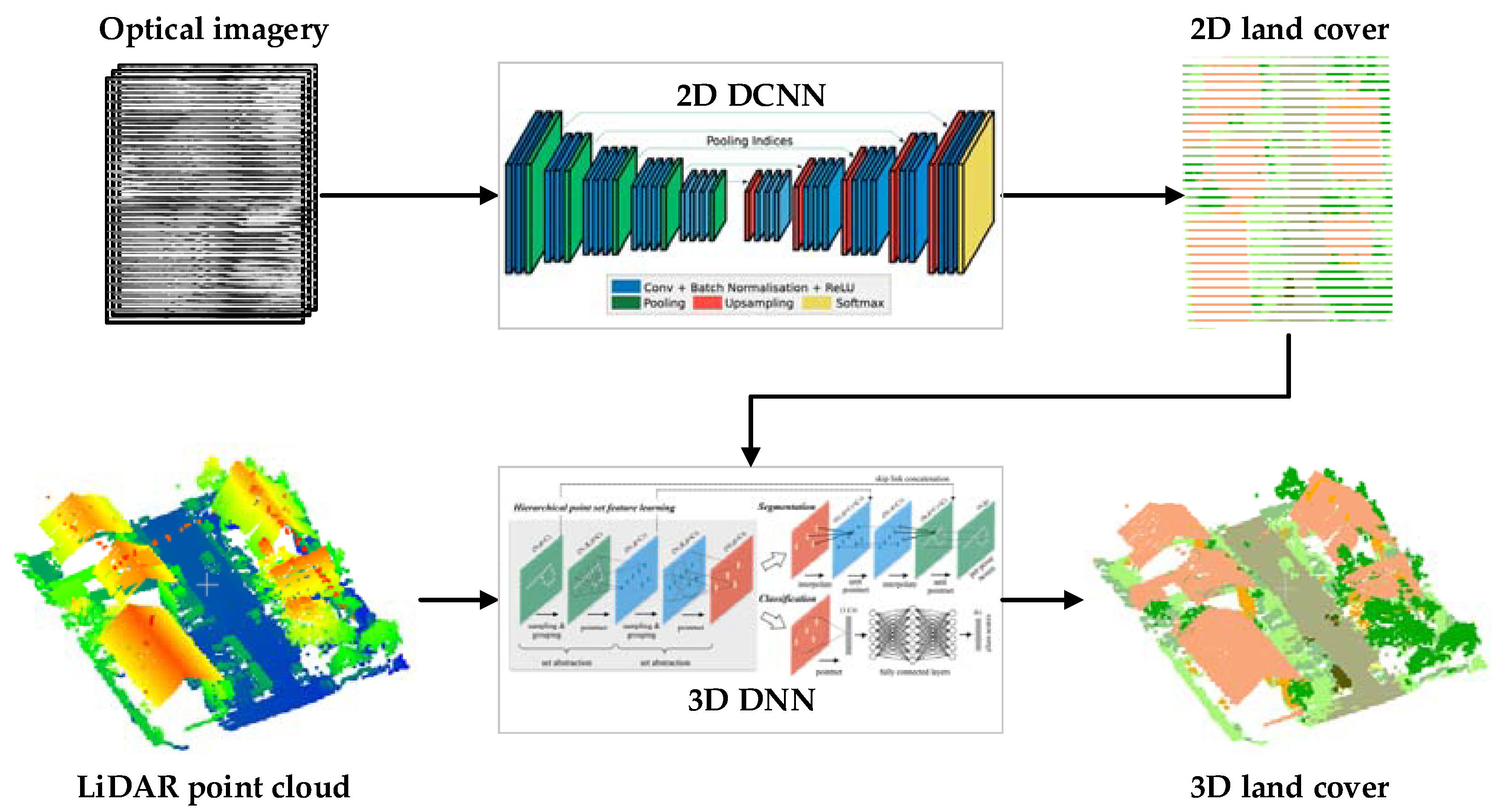
The proposed prior-level fusion of LiDAR point clouds and optical imagery for three-dimensional urban land cover classification includes three main parts (Figure 2).

(1) Obtain two-dimensional land cover, namely prior knowledge, from the optical image (see Section 2.1). Here, optical imagery is classified by a deep convolutional neural network (DCNN), and the result of DCNN is the probability belonging to each class. The probability is considered as prior to the subsequent three-dimensional classification. The DCNN used in this study was SegNet [33].

(2) Assign the prior knowledge to the LiDAR point cloud (see Section 2.2). The prior derived from the optical imagery is two-dimensional; however, the LiDAR point cloud is three-dimensional. These can be linked through their coordinates. We use $\left(x, y\right)$ of the LiDAR point to search for its nearest pixel in the optical image to obtain a prior.

(3) Classify the LiDAR point cloud that has been assigned the prior knowledge to produce the three-dimensional urban land cover by three-dimensional DNN (see Section 2.3). The LiDAR point cloud is sparse and irregular, which renders traditional convolution unusable. PointNet++ represents pioneering work on point clouds to overcome this problem [34] and was used to classify urban LiDAR point clouds in this study where the hyper-parameter of PointNet++ was redesigned.

2.1. Obtaining Prior Knowledge from Optical Image Using Deep Convolutional Neural Network (DCNN)

Obtaining prior knowledge corresponds to optical image semantic segmentation, which gives every pixel a classification vector and can be accomplished by using fully convolutional networks (FCNs), a popular DCNN. There are many FCNs, such as UNet [35], SegNet [33], and PSPNet [36]. Among these, SegNet exhibits a good balance between operating efficiency, required memory, and classification accuracy, and has high efficiency in space and time utilization [33]. Thus, we selected SegNet as the base model for optical imagery semantic segmentation.

SegNet consists of a trainable encoding network and a corresponding decoding network, with a pixel-level Softmax classifier after the decoding network. The encoding network is the convolutional neural network VGG-16 [37] without a fully connected network, which can extract encoding features. The encoding network contains five groups of encoders. Each group uses a convolutional layer, a batch normalization layer, a rectified linear unit (ReLU) activation layer, and a max-pooling layer to extract features and expand their receptive field. The output of the encoding network is 1/32 of the original image. The parameters in the encoding network can be initialized by a VGG-16 pre-trained model, which is convenient for learning an improved classifier on the remote sensing data.

Unlike the encoding network, the decoding network up-samples low resolution features (1/32 of the original image) through the up-sampling layer, convolutional layer, batch normalization layer, and ReLU activation layer to obtain a feature image that is of the same size as the original image. The up-sampling layer uses indices of corresponding max-pooling to obtain sparse features with higher resolution, and the sparse features are densified through a convolution layer, a batch normalization layer, and a ReLU activation layer. The featured image with the same size as the original image is classified by the pixel-level Softmax classifier to obtain the needed prior for each pixel.

2.2. Assigning Prior Knowledge to the Light Detection and Ranging (LiDAR) Point Cloud

The prior knowledge obtained from the optical imagery are raster data that is indexed by pixel $\left(r,c\right)$, where $r$ is the row and $c$ is the column of pixel relative to the upper left corner of the raster. Each pixel contains classification probability vectors $p$.

$$p=\left(p_1,p_2\dots , p_k\right)$$

(1)

where k indicates the k type of two-dimensional land cover.

We can use the x and y in the coordinates $\left(x,y,z\right)$ of a LiDAR point to calculate the corresponding row and column $\left(r^{\prime },c^{\prime }\right)$ in the raster data as follows:

$$r^{\prime }=\frac{\lfloor x-X\rfloor }{gsd}, c^{\prime }=\frac{\lfloor y-Y\rfloor }{gsd}$$

(2)

where $\left(X,Y\right)$ are the coordinates of the upper left corner of the raster, and gsd is the ground sample distance, namely, the spatial resolution of the raster

The prior value is assigned to the LiDAR point cloud according to its corresponding calculated $\left(r^{\prime }, c^{\prime }\right)$ value. Then, a point in the LiDAR point cloud can be represented by $\left(x,y,z,p_1,p_2,\dots ,p_k\right)$ instead of $\left(x,y,z\right)$, which establishes a link between the two-dimensional and three-dimensional land cover classification.

2.3. Classification of LiDAR Point Cloud Assigned Prior to Three-Dimensional Deep Neural Network (DNN)

Unlike optical imagery, whose regular grid makes it convenient for convolution and automatic feature extraction in the end-to-end framework, a LiDAR point cloud is disordered and irregular, which make it difficult to design DNNs for learning point cloud features. In PointNet, an MLP-Max operation is designed to overcome the difficulty, where a multi-layer perceptron (MLP) is operated on $\left(x,y,z,p_1,p_2,\dots ,p_k\right)$ to extract a feature for every point, and then maximum pooling is used to summarize the extracted features of all points within the spherical neighborhood to a single vector [15].

PointNet++ extends PointNet to extract hierarchical point features and forms an encoder-decoder structure for point cloud semantic segmentation [34]. PointNet++ includes sampling and grouping, feature extraction, up-sample, and feature set propagation layers. The sampling and grouping layer use the farthest point sampling method to obtain abstract points and their spherical neighborhood. The feature extraction layer uses PointNet to extract abstract features for abstract points. The sampling and grouping layer and feature extraction layer are repeated to form an encoder network. For point cloud semantic segmentation, a decoder network is needed to up-sample the abstract points into their original point cloud size. The up-sample layer is accomplished by the distance-based interpolation and level skip link, and the features of the up-sample layer are readjusted through a feature set propagation layer (i.e., a PointNet). Finally, the Softmax classifier is used to derive the three-dimensional classification result.

PointNet++ was originally designed for small-scale indoor point clouds and cannot be directly used for urban LiDAR point clouds. Therefore, we redesigned the hyper-parameters of every layer in PointNet++ (

Table 1. Redesigned hyper-parameters in PointNet++ for urban light detection and ranging (LiDAR) point clouds.

Layer	Parameter
Sampling and grouping	N = 1024, r = 2, K = 32
Feature extraction	[32, 32, 64]
Sampling and grouping	N = 256, r = 4, K = 32
Feature extraction	[64, 64, 128]
Sampling and grouping	N = 64, r = 8, K = 32
Feature extraction	[128, 128, 256]
Sampling and grouping	N = 16, r = 16, K = 32
Feature extraction	[256, 256, 512]
Feature set propagation	[256, 256]
Feature set propagation	[256, 256]
Feature set propagation	[256, 128]
Feature set propagation	[128, 128, 128]

Notes: N is the number of abstract points, r is the radius of the spherical neighborhood, K is the maximum number of used points in a local region, and numbers in [·] represent multi-layer perceptron (MLP) in PointNet.

).

2.4. Fusion Strategies on Three Other Different Levels

To evaluate our proposed prior-level fusion strategy, we compare it with three other commonly used fusion strategies including point-level, feature-level, and decision-level fusion strategies [30]. We accomplished all the fusion strategies under the DNN framework by using SegNet and PointNet++ to ensure the fairness of the comparison as much as possible (Figure 3).

The point-level fusion strategy assigns multispectral information from optical imagery to the points and then trains the classifier using three-dimensional DNN to classify the point cloud with spectral information (point level in Figure 3). The feature-level fusion strategy first concatenates the features extracted from the multispectral image by DCNN and the features extracted from the LiDAR point cloud by three-dimensional DNN, and then the concatenated features are fed to an MLP to derive the three-dimensional land cover classification result (feature-level in Figure 3). Unlike point-level and feature-level fusion, the decision-level fusion strategy directly classifies the optical imagery and LiDAR point cloud to obtain two- and three-dimensional classification results, which are then combined using a heuristic fusion rule (decision-level in Figure 3). The heuristic fusion rule used in this study was to update the probability of a three-dimensional classification results based on the two-dimensional classification results.

The updating procedure included two steps: (1) three-dimensional classification probabilities are multiplied by two-dimensional classification probabilities according to land cover type; for example, the probabilities of a façade and roof in three-dimensional land cover are multiplied by the probability of a building in two-dimensional land cover, and the probabilities of a shrub and tree in three-dimensional land cover are multiplied by the probability of vegetation in two-dimensional land cover; (2) then, multiplied probabilities normalized to ensure that the sum of probabilities belonging to three-dimensional land cover type is one. The final classification result of decision-level fusion strategies is determined by the type whose probability is the maximum.

3. Experimental Data and Results

3.1. Experimental Data

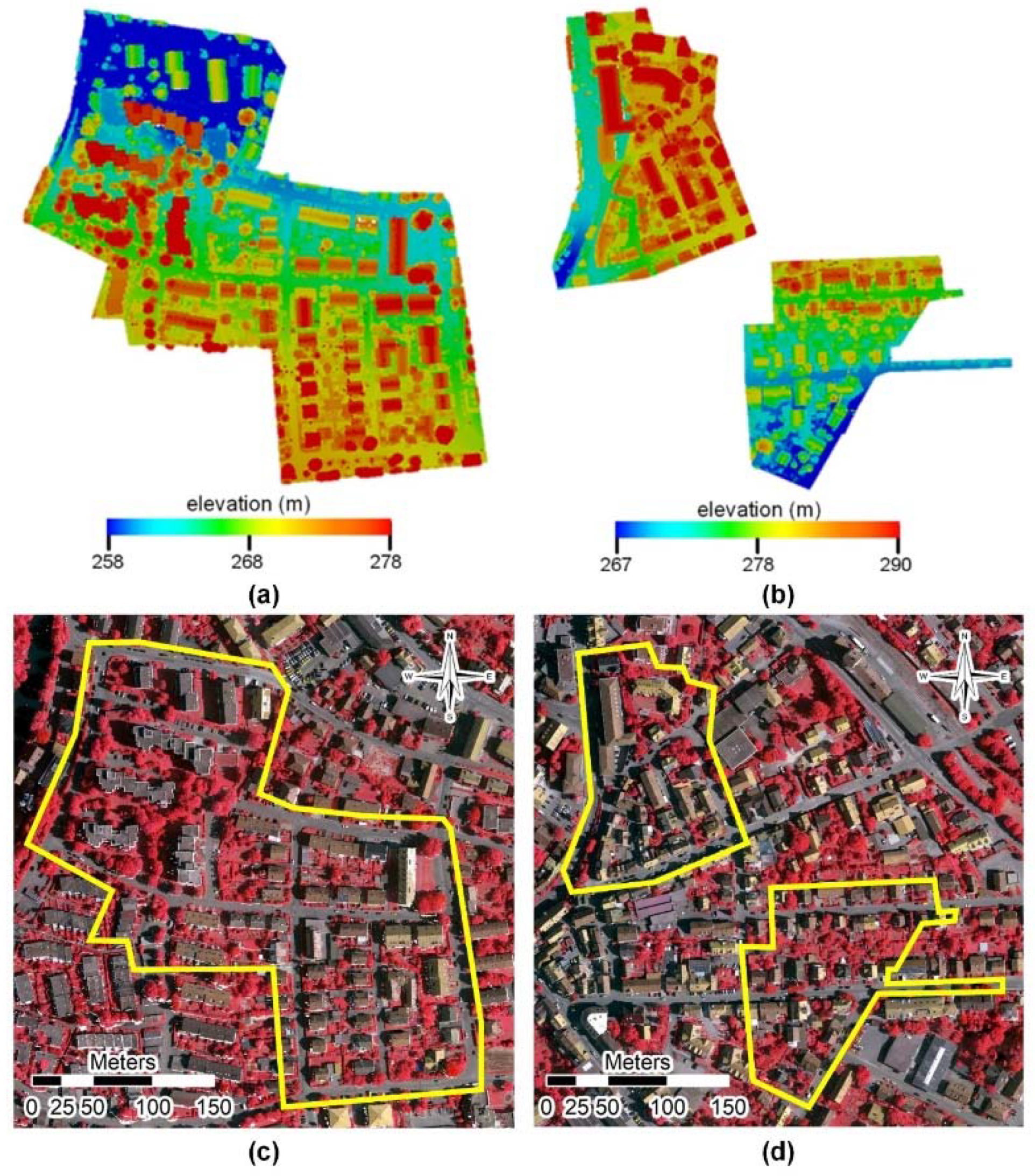
The LiDAR point cloud and optical imagery used in this experiment were provided by the International Society for Photogrammetry and Remote Sensing (ISPRS) and downloaded from https://www.isprs.org/education/benchmarks.aspx on 12 July 2019. The LiDAR point cloud is an airborne LiDAR dataset that was collected by Leica Geosystems in Vaihingen using the Leica ALS50 system with a 45° field of view. Its geographic coordinate system is WGS84 and the projected coordinate system is UTM-32N. The average point density is 8 pts/m². The ISPRS working group labeled some parts of these data as training and testing data to evaluate the three-dimensional land cover classification (Figure 4a,b). The labeled categories are power line, low vegetation, impervious ground, car, fence, roof, façade, shrub, and tree.

The optical multispectral imagery provided by the ISPRS is ortho photographic images comprising three bands: near-infrared, red, and green (IR-R-G; Figure 4c,d). The spatial resolution of the optical multispectral image is 1 m. The projected coordinate system of the orthophoto images is the same as the airborne LiDAR point cloud. Thus, registration of LiDAR data and optical imagery was not needed in this experiment. The ISPRS working group selected 16 blocks from Vaihingen’s ortho photographic images and manually labeled six categories including impervious surface, building, low vegetation, tree, car, and background. The background includes water bodies and other objects.

To simplify the design of the rule of the decision-level fusion strategy, the categories used for the point cloud were low vegetation, shrub, tree, impervious surface, façade, and roof. The categories used for the optical imagery were impervious surface, building, low vegetation, and tree.

3.2. Details of Experimental Setting

The optical imagery used in this experiment has three spectral bands. SegNet can be directly used and its encoder network parameters were initialized using a pre-trained VGG-16 model. We randomly selected 12 blocks of the optical image to fine-tune SegNet and set aside four other blocks for evaluation. The input image block for SegNet was a randomly cropped 256 × 256 image unit. For training SegNet, we set a batch size of 16, and the parameter optimizer selected the Stochastic Gradient Descent (SGD) method. The loss function used in SegNet was the weighted cross-entropy loss, calculated as:

$$loss\left(y_{\mathrm{p}}, y_{\mathrm{g}}\right)=w\left[y_{\mathrm{g}}\right]\left(-y_p\left[y_{\mathrm{g}}\right]+\log \left({\displaystyle \sum }_j\exp \left(y_{\mathrm{p}}\left[j\right]\right)\right)\right)$$

(3)

where $y_{\mathrm{p}}$ is the predicted probability vector, $y_{\mathrm{g}}$ is the ground truth, and $w$ is the weight vector for every class, which is calculated by dividing the class frequency by the median of all class frequencies.

Although the three-dimensional geometry information $\left(x,y,z\right)$ of the LiDAR point cloud was the same for all four fusion strategies, we trained different PointNet++ models because the different strategies have different auxiliary information. First, baseline trained the PointNet++ by only using three-dimensional geometry information. The point-level fusion strategy trained PointNet++ using geometry and spectral information [i.e., (x, y, z, IR, R, G)]. The prior-level fusion strategy trained PointNet++ using geometry and prior information [i.e., (x, y, z, p₁, p₂, …, p_k)]. The batch size of these models was set to 16, and the parameters were initialized using the Xavier initializer provided in TensorFlow. The optimizer was the adaptive moment estimation method. The loss function was the weighted cross-entropy loss (Equation (3)). The learning rate decreased by an exponential decay. The input unit of PointNet++ was a point set that had 8192 points. Thus, we split the LiDAR training data (Figure 4a) into 30 × 30 m blocks and resampled them into 8192 points for training PointNet++. When classifying the LiDAR testing data (Figure 4b), we also down-sampled the original data using the same procedure for the training data to obtain the classification result of down-sampled point cloud by using the trained PointNet++ model; we then classified every point of testing data to the type of its nearest point in the down-sampled point cloud.

3.3. Classification of the Prior-Level Strategy with other Fusion Strategies

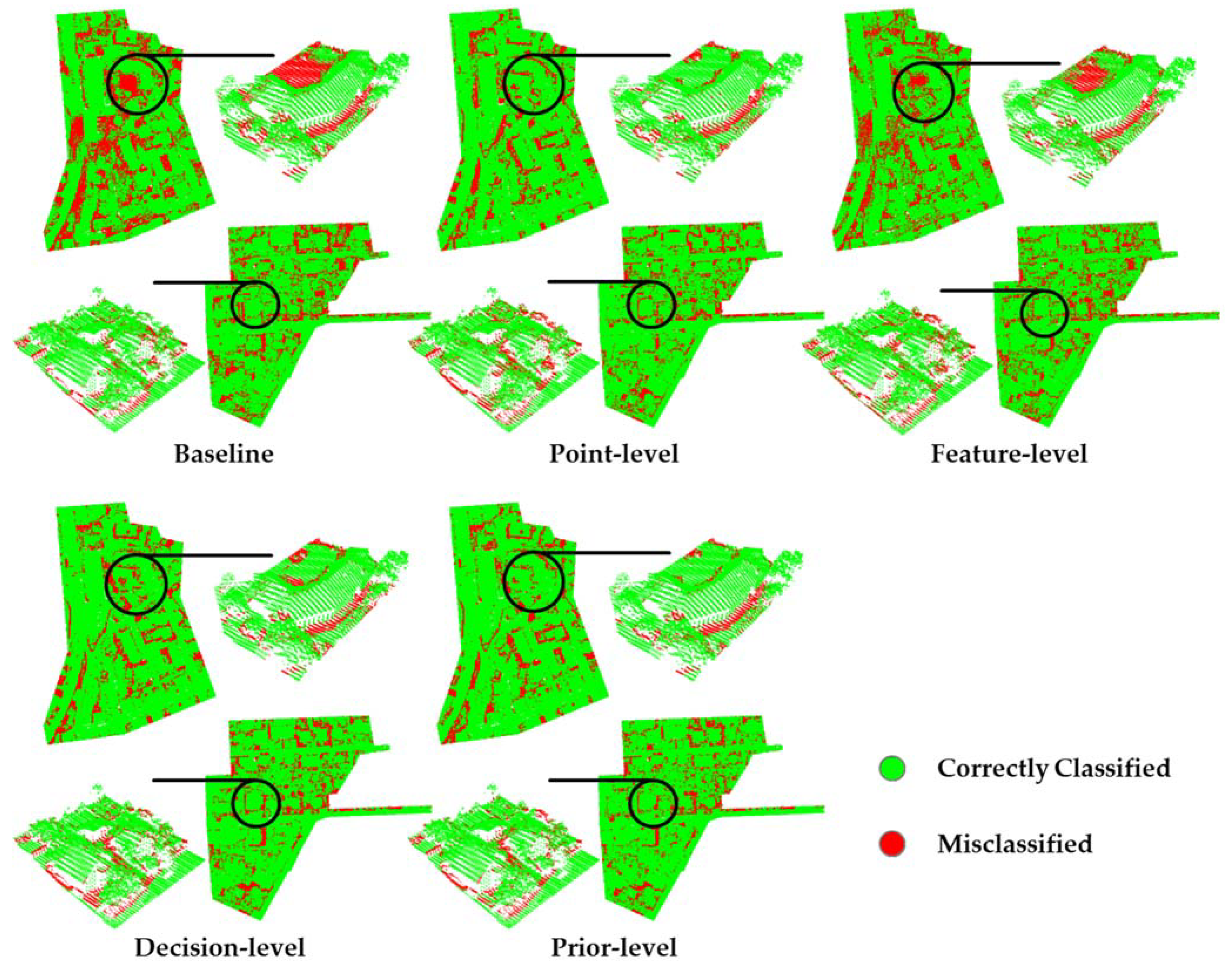
Figure 5 shows the ground truth and results of the four fusion strategies. All four fusion strategies achieved acceptable performance. In particular, three dominant geo-objects, namely tree, impervious surface, and roof, presented high accuracy (

Table 2. Classification performance of the baseline and four fusion strategies.

Classification Performance		Baseline	Point-Level	Feature-Level	Decision-Level	Prior-Level
Low vegetation	Precision	73.18	84.27	75.97	91.91	89.83
	Recall	63.58	68.40	66.94	65.46	72.69
	F1-score	68.04	75.51	71.17	76.46	80.36
Shrub	Precision	33.25	31.12	34.51	34.50	35.58
	Recall	71.60	58.61	58.15	66.02	66.19
	F1-score	45.42	40.66	43.31	45.32	46.28
Tree	Precision	77.37	83.02	75.38	85.21	85.45
	Recall	74.68	80.21	81.70	80.67	80.74
	F1-score	76.00	81.59	78.41	82.88	83.03
Impervious surface	Precision	80.59	86.61	81.64	84.23	88.38
	Recall	79.99	91.99	83.42	95.99	94.74
	F1-score	80.29	89.22	82.52	89.73	91.45
Roof	Precision	94.27	94.68	95.23	96.57	96.52
	Recall	86.27	91.73	40.84	91.45	91.27
	F1-score	90.10	93.18	90.25	93.94	93.82
Facade	Precision	49.04	41.31	85.76	42.73	44.08
	Recall	67.69	53.69	65.31	71.88	70.90
	F1-score	56.87	46.69	50.25	53.60	54.36
Weighted Average	Precision	76.73	81.45	77.51	83.70	84.39
	Recall	74.62	79.86	76.22	81.12	82.47
	F1-score	75.08	80.15	76.46	81.35	82.79

). Figure 6 shows the error distribution for different fusion strategies. Compared with the baseline, the red area in the other classification error distribution plots is smaller, indicating that the four fusion strategies had fewer classification errors and improved overall classification accuracy. The increase in overall classification accuracy was 5.24% for the point-level, 1.60% for the feature-level, 6.50% for the decision-level, and 7.85% for the prior-level (Table 2). The F1-scores of the decision-level and prior-level were >80%. Among the fusion strategies, prior-level had the highest accuracy and lowest error (Table 2, Figure 5 and Figure 6).

4. Discussion

Studying the heterogeneity of urban landscapes is important for managing the urban environment, and requires a three-dimensional urban land cover product. Three-dimensional LiDAR classification is a fundamental task for producing this three-dimensional land cover product. Traditionally, LiDAR data always act as auxiliary data in two-dimensional land cover classification where an optical image is the core data, to improve accuracy. We fused optical images into LiDAR classification and found that the three-dimensional accuracy could also be improved by the fusion (Table 2, Figure 5). Among the different fusion strategies, our proposed prior-fusion approach had the highest accuracy. The phenomenon was analyzed using the loss during the training process (see Section 4.1). Moreover, we checked the error region in Figure 6 to identify the data bottleneck in the three-dimensional land cover classification (see Section 4.2). Finally, we compared the results with other methods to indicate the limitations of the approach and the scope (see Section 4.3).

4.1. Loss Variation during Training

The loss used in this study was cross-entropy loss, which measures the difference between two probability distributions (Equation (3)), indicating that the lower the loss, the better the prediction of the model; loss variation is an important indication for the DNN training process. During the training process, the loss was decreased by updating the parameters of the DNN (Figure 7 and Figure 8). Note that there was no overall loss in the decision-level classification, which included the loss with the baseline and the loss with the SegNet (Figure 8). When the training loss was stable, the largest loss occurred with the feature-level, followed by the baseline, point-level, and prior-level. Moreover, the prior-level offered the fastest convergence because it directly used the two-dimensional land cover classification result, which contained semantic information. When the test loss was stable, the largest loss occurred with the baseline, followed by the feature-level, point-level, and prior-level, consistent with the overall accuracy of the classification in the prediction results. These phenomena imply that, after embedding the information from the optical imagery, the loss becomes smaller and reaches a stable state faster.

Of the two losses with the decision-level, irrespective of training or testing, the loss with baseline was greater than the loss with SegNet (Figure 7 and Figure 8), confirming that it is reasonable to train different DNN for the optical imagery and LiDAR point cloud separately, and that the prior-level fusion strategy can make use of the two-dimensional neural network pre-training model in three-dimensional land cover classification when the training data are insufficient. The training loss with the feature-level was greatest because the MLP classifier in the feature-level only had two layers, and a dropout was added, resulting in a weak learning capability.

4.2. Detailed Analysis of the Error Region

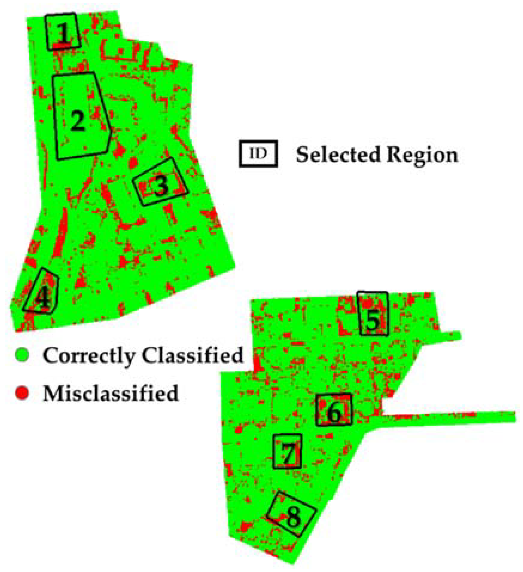
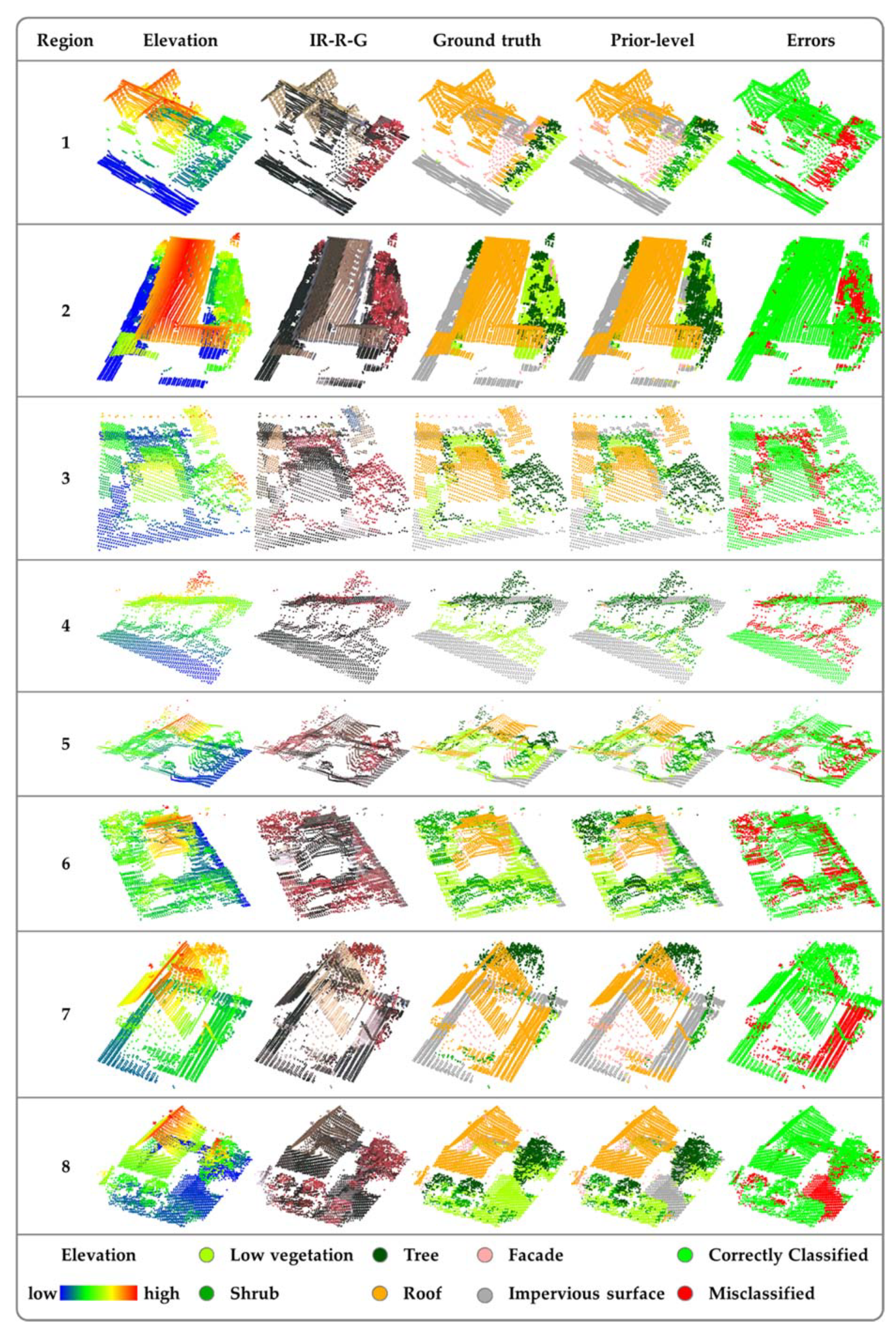
Among all fusion strategies, the error region of the prior-level was smallest (Figure 6), and the performance of the prior-level fusion strategy was highest (Table 2 and Figure 5). Therefore, we selected eight typical regions that were misclassified by the prior-level fusion strategy (Figure 9). Generally, the elevation of the misclassified regions varied abruptly (Figure 10). For example, there were significant elevation differences between grassland and adjoining impervious surface (i.e., region 1 in Figure 10), and between the bottom of a building and the adjacent grassland (i.e., a narrow ditch in region 2 of Figure 10). Grassland was misclassified as shrubs in region 4 of Figure 10, because the elevation difference suddenly increased after the road bifurcated. Compared with regions with gentle elevation change, the density of the point cloud in these areas was lower, and the distribution of the point cloud was sparser. Thus, there were insufficient points to resolve local features, likely leading to the misclassification.

Errors also occurred when two geo-objects of the same type had large elevation differences. For example, when high and low trees were mixed, the prior-level strategy misclassified some of the smaller trees as shrubs (i.e., regions 3 and 5 in Figure 10). Some shrubs were also misclassified as trees (i.e., region 6 in Figure 10). Similarly, when two buildings were connected and the lower roof was near the ground level, the lower roof was likely to be misclassified as ground (i.e., region 7 in Figure 10). These errors may be significantly reduced by incorporating vertical information (i.e., tree trunks and building façades), such that integration of multi-platform LiDAR, such as backpack LiDAR and vehicle LiDAR, is necessary for three-dimensional urban land cover classification. Although some errors existed in the classification results of the prior-level fusion strategy, the majority situations were more accurate than the manually labeled results (i.e., region 8 in Figure 10).

4.3. Comparison with Other Methods

The purpose of this study was to explore the fusion strategy for LiDAR point clouds and optical imagery for three-dimensional urban land cover classification. Therefore, we used the basic PointNet++ and SegNet models. Apart from PointNet++, some machine learning methods were also used for point cloud classification. To compare our prior-level fusion strategy with these methods and determine the limitations of our method, we used the prior-level fusion strategy to classify the ISPRS LiDAR point cloud into the nine original categories and then compared it with other methods (

Table 3. Comparison of fusion-level strategy results with other methods.

Classification Result	Non-Deep Learning				Deep Learning
	ISS_7	UM	HM1	LUH	RIT1	WhuY4	PointCNN	A-XCRF	Ours
Power line	54.4	46.1	69.8	59.6	37.5	42.5	61.5	63.0	27.5
Low vegetation	65.2	79.0	73.8	77.5	77.9	82.7	82.7	82.6	79.8
Impervious surface	85.0	89.1	91.5	91.1	91.5	91.4	91.8	91.9	91.9
Car	57.9	47.7	58.2	73.1	73.4	74.7	75.8	74.9	71.4
Fence	28.9	05.2	29.9	34.0	18.0	53.7	35.9	39.9	29.0
Roof	90.9	92.0	91.6	94.2	94.0	94.3	92.7	94.5	92.7
Façade	-	52.7	54.7	56.3	49.3	53.1	57.8	59.3	53.8
Shrub	39.5	40.9	47.8	46.6	45.9	47.9	49.1	50.8	44.3
Tree	75.6	77.9	80.2	83.1	82.5	82.8	78.1	82.7	82.3
Average F1	55.3	59.0	66.4	68.4	63.3	69.2	69.5	71.1	63.6
Overall Accuracy	76.2	80.8	80.5	81.6	81.6	84.9	83.3	85.0	81.4

).

The methods in Table 3 are divided into non-deep learning and deep learning. ISS_7 [38] first extracts the super-prime with the help of point cloud geometry and optical spectral information, and then uses machine learning to classify the super-prime. UM [39] uses the multiple attributes of the point cloud (intensity, echo number, etc.), texture features (locally fitted surfaces), and morphological features (differential morphological profile lines) to train a one-to-one class machine learning strategy classifier. HM_1 uses k-nearest neighbors (KNN) to select domain points to extract features, and then uses a conditional random field (CRF) to complete the context classification. LUH [40] uses high-order CRF to complete the classification with the help of extracted super-primes. RIT_1 [19] extracts the ground to obtain a normalized elevation and then uses PointNet to process the LiDAR point cloud fused with optical imagery. WhuY4 [41] uses a multi-scale CNN to process feature images obtained from LiDAR point clouds. The features used include normalized elevation, intensity, normal vector, and local plane features. PointCNN is the baseline in the A-XCR method [42], and its processing method is similar to that of the point-level fusion strategy described in this paper. Based on PointCNN training, A-XCR introduces an error smoothing process generated by CRF to avoid the over-fitting of PointCNN.

The deep learning methods were superior to the non-deep learning methods (Table 3), and by normalizing the elevation of the LiDAR point cloud, extracting some features for deep learning can achieve higher accuracy. Furthermore, using an advanced neural network architecture, such as PointCNN that uses a dilated convolution technique to obtain multiple models and integrates these to get superior results, can also improve accuracy. Thus, in the future, we plan to embed PointCNN or other more advanced three-dimensional classification networks, such as KPConv [43], into the prior-level fusion strategy; such embedding will be simple owing to the serial form of the proposed prior-level fusion strategy (Figure 2).

5. Conclusions

In this study, a novel prior-level fusion strategy of LiDAR point clouds and optical imagery for three-dimensional land cover classification was proposed and compared with other fusion strategies, namely point-level, feature-level, and decision-level. The proposed prior-level fusion strategy builds a link between two-dimensional and three-dimensional land cover through the prior knowledge obtained from the optical imagery. The point-level fusion strategy directly assigns multispectral information of the optical imagery to the point cloud, and classifies the point cloud with multispectral information. The feature-level fusion strategy concatenates the features extracted from the optical image and the features from the LiDAR point cloud, and then the concatenated feature is used to obtain classification results. The decision-level fusion strategy fuses the results of two-dimensional land cover from optical imagery and three-dimensional land cover from a LiDAR point cloud based on the heuristic rule. The experimental results using ISPRS data show that the proposed prior-level fusion strategy delivers the best performance, which is manifested mainly in the lowest losses in the training process and highest F1-score (82.79%) in the classification results. The F1-score of point-level, feature-level, decision-level, and prior-level were 80.15%, 76.46%, 81.35%, and 82.79%, respectively.

Through detailed analysis of the error distribution of the prior-level fusion strategy, we found that some errors arose due to date problems, such as the airborne LiDAR point cloud being very sparse at locations where elevation changed abruptly, as airborne LiDAR lacks vertical information. If other platforms of LiDAR, such as backpack LiDAR and vehicle LiDAR, were integrated with the airborne LiDAR, more reliable three-dimensional urban land cover could be achieved, which would help urban ecology research. On the other hand, since the pioneering work of PointNet++, a few three-dimensional deep learning structures with better performance have emerged to encode the point cloud neighborhood relationship. We anticipate that it will be necessary to adopt a more advanced neural network structure in the prior-level fusion strategy to improve the performance of three-dimensional land cover classification.

References

1. Cadenasso, M.L.; Pickett, S.T.A.; Schwarz, K. Spatial heterogeneity in urban ecosystems: Reconceptualizing land cover and a framework for classification. Front. Ecol. Environ. 2007, 5, 80–88. [Google Scholar] [CrossRef]
2. Grimm, N.B.; Faeth, S.H.; Golubiewski, N.E.; Redman, C.L.; Wu, J.; Bai, X.; Briggs, J.M. Global Change and the Ecology of Cities. Science 2008, 319, 756–760. [Google Scholar] [CrossRef] [Green Version]
3. Zhu, Z.; Zhou, Y.; Seto, K.C.; Stokes, E.C.; Deng, C.; Pickett, S.T.; Taubenböck, H. Understanding an urbanizing planet: Strategic directions for remote sensing. Remote Sens. Environ. 2019, 228, 164–182. [Google Scholar] [CrossRef]
4. Wentz, E.A.; York, A.M.; Alberti, M.; Conrow, L.; Fischer, H.; Inostroza, L.; Jantz, C.; Pickett, S.T.; Seto, K.C.; Taubenböck, H. Six fundamental aspects for conceptualizing multidimensional urban form: A spatial mapping perspective. Landsc. Urban Plan. 2018, 179, 55–62. [Google Scholar] [CrossRef]
5. Stewart, I.D.; Oke, T.R. Local Climate Zones for Urban Temperature Studies. Bull. Am. Meteorol. Soc. 2012, 93, 1879–1900. [Google Scholar] [CrossRef]
6. Wang, V.; Gao, J. Importance of structural and spectral parameters in modelling the aboveground carbon stock of urban vegetation. Int. J. Appl. Earth Obs. Geoinform. 2019, 78, 93–101. [Google Scholar] [CrossRef]
7. Mallet, C.; Bretar, F.; Roux, M.; Soergel, U.; Heipke, C. Relevance assessment of full-waveform lidar data for urban area classification. ISPRS J. Photogramm. Remote Sens. 2011, 66, S71–S84. [Google Scholar] [CrossRef]
8. Guo, B.; Huang, X.; Zhang, F.; Sohn, G. Classification of airborne laser scanning data using JointBoost. ISPRS J. Photogramm. Remote Sens. 2015, 100, 71–83. [Google Scholar] [CrossRef]
9. Liu, X.; Chen, Y.; Li, S.; Cheng, L.; Li, M. Hierarchical Classification of Urban ALS Data by Using Geometry and Intensity Information. Sensors 2019, 19, 4583. [Google Scholar] [CrossRef] [PubMed] [Green Version]
10. Rusu, R.B.; Blodow, N.; Beetz, M. Fast Point Feature Histograms (FPFH) for 3D registration. In Proceedings of the 2009 IEEE International Conference on Robotics and Automation, Kobe, Japan, 12–17 May 2009; pp. 3212–3217. [Google Scholar]
11. Blomley, R.; Weinmann, M.; Leitloff, J.; Jutzi, B. Shape distribution features for point cloud analysis—A geometric histogram approach on multiple scales. ISPRS Ann. Photogramm. Remote Sens. Spat. Inf. Sci. 2014, II-3, 9–16. [Google Scholar] [CrossRef] [Green Version]
12. Osada, R.; Funkhouser, T.; Chazelle, B.; Dobkin, D. Shape distributions. ACM Trans. Graph. 2002, 21, 807–832. [Google Scholar] [CrossRef]
13. Weinmann, M.; Urban, S.; Hinz, S.; Jutzi, B.; Mallet, C. Distinctive 2D and 3D features for automated large-scale scene analysis in urban areas. Comput. Graph. 2015, 49, 47–57. [Google Scholar] [CrossRef]
14. Dittrich, A.; Weinmann, M.; Hinz, S. Analytical and numerical investigations on the accuracy and robustness of geometric features extracted from 3D point cloud data. ISPRS J. Photogramm. Remote Sens. 2017, 126, 195–208. [Google Scholar] [CrossRef]
15. Qi, C.R.; Su, H.; Mo, K.; Guibas, L.J. PointNet: Deep Learning on Point Sets for 3D Classification and Segmentation. In Proceedings of the IEEE Conference on Computer Vision and Pattern Recognition (CVPR), Honolulu, HI, USA, 21–26 July 2017. [Google Scholar]
16. Li, Y.; Bu, R.; Sun, M.; Wu, W.; Di, X.; Chen, B. Pointcnn: Convolution on x-transformed points. Adv. Neural 2018, 31, 820–830. [Google Scholar]
17. Graham, B.; Engelcke, M.; van der Maaten, L. 3D Semantic Segmentation with Submanifold Sparse Convolutional Networks. In Proceedings of the 2018 IEEE/CVF Conference on Computer Vision and Pattern Recognition, Salt Lake City, UT, USA, 18–22 June 2018; pp. 9224–9232. [Google Scholar]
18. Guo, Y.; Wang, H.; Hu, Q.; Liu, H.; Liu, L.; Bennamoun, M. Deep Learning for 3D Point Clouds: A Survey. IEEE Trans. Pattern Anal. Mach. Intell. 2020, 43, 4338–4364. [Google Scholar] [CrossRef]
19. Yousefhussien, M.; Kelbe, D.J.; Ientilucci, E.J.; Salvaggio, C. A multi-scale fully convolutional network for semantic labeling of 3D point clouds. ISPRS J. Photogramm. Remote Sens. 2018, 143, 191–204. [Google Scholar] [CrossRef]
20. Zhang, R.; Li, G.; Li, M.; Wang, L. Fusion of images and point clouds for the semantic segmentation of large-scale 3D scenes based on deep learning. ISPRS J. Photogramm. Remote Sens. 2018, 143, 85–96. [Google Scholar] [CrossRef]
21. Zhang, J.; Lin, X. Advances in fusion of optical imagery and LiDAR point cloud applied to photogrammetry and remote sensing. Int. J. Image Data Fusion 2017, 8, 1–31. [Google Scholar] [CrossRef]
22. Ghamisi, P.; Gloaguen, R.; Atkinson, P.M.; Benediktsson, J.A.; Rasti, B.; Yokoya, N.; Wang, Q.; Hofle, B.; Bruzzone, L.; Bovolo, F.; et al. Multisource and Multitemporal Data Fusion in Remote Sensing: A Comprehensive Review of the State of the Art. IEEE Geosci. Remote Sens. Mag. 2019, 7, 6–39. [Google Scholar] [CrossRef] [Green Version]
23. Singh, K.K.; Vogler, J.B.; Shoemaker, D.A.; Meentemeyer, R.K. LiDAR-Landsat data fusion for large-area assessment of urban land cover: Balancing spatial resolution, data volume and mapping accuracy. ISPRS J. Photogramm. Remote Sens. 2012, 74, 110–121. [Google Scholar] [CrossRef]
24. Paisitkriangkrai, S.; Sherrah, J.; Janney, P.; Hengel, A.V.-D. Effective semantic pixel labelling with convolutional networks and Conditional Random Fields. In Proceedings of the 2015 IEEE Conference on Computer Vision and Pattern Recognition Workshops (CVPRW), Boston, MA, USA, 7–12 June 2015; pp. 36–43. [Google Scholar]
25. Audebert, N.; Le Saux, B.; Lefèvre, S. Beyond RGB: Very high resolution urban remote sensing with multimodal deep networks. ISPRS J. Photogramm. Remote Sens. 2018, 140, 20–32. [Google Scholar] [CrossRef] [Green Version]
26. Rasti, B.; Ghamisi, P.; Gloaguen, R. Hyperspectral and LiDAR Fusion Using Extinction Profiles and Total Variation Component Analysis. IEEE Trans. Geosci. Remote Sens. 2017, 55, 3997–4007. [Google Scholar] [CrossRef]
27. Debes, C.; Merentitis, A.; Heremans, R.; Hahn, J.; Frangiadakis, N.; Van Kasteren, T.; Liao, W.; Bellens, R.; Pizurica, A.; Gautama, S.; et al. Hyperspectral and LiDAR Data Fusion: Outcome of the 2013 GRSS Data Fusion Contest. IEEE J. Sel. Top. Appl. Earth Obs. Remote Sens. 2014, 7, 2405–2418. [Google Scholar] [CrossRef]
28. Audebert, N.; Le Saux, B.; Lefèvre, S. Semantic Segmentation of Earth Observation Data Using Multimodal and Multi-Scale Deep Networks; Lai, S., Lepetit, V., Nishino, K., Sato, Y., Eds.; Asian Conference on Computer Vision; Springer: Cham, Germany, 2017; pp. 180–196. [Google Scholar] [CrossRef] [Green Version]
29. Guo, L.; Chehata, N.; Mallet, C.; Boukir, S. Relevance of airborne lidar and multispectral image data for urban scene clas-sification using Random Forests. ISPRS J. Photogramm. Remote Sens. 2011, 66, 56–66. [Google Scholar] [CrossRef]
30. Ghassemian, H. A review of remote sensing image fusion methods. Inf. Fusion 2016, 32, 75–89. [Google Scholar] [CrossRef]
31. Ji, S.; Wei, S.; Lu, M. Fully Convolutional Networks for Multisource Building Extraction from an Open Aerial and Satellite Imagery Data Set. IEEE Trans. Geosci. Remote Sens. 2019, 57, 574–586. [Google Scholar] [CrossRef]
32. Demir, I.; Koperski, K.; Lindenbaum, D.; Pang, G.; Huang, J.; Basu, S.; Hughes, F.; Tuia, D.; Raskar, R. DeepGlobe 2018: A Challenge to Parse the Earth through Satellite Images. In Proceedings of the 2018 IEEE/CVF Conference on Computer Vision and Pattern Recognition Workshops (CVPRW), Salt Lake City, UT, USA, 18–22 June 2018; pp. 172–181. [Google Scholar]
33. Badrinarayanan, V.; Kendall, A.; Cipolla, R. Segnet: A deep convolutional encoder-decoder architecture for image seg-mentation. IEEE Trans. Pattern Anal. Mach. Intell. 2017, 39, 2481–2495. [Google Scholar] [CrossRef]
34. Qi, C.R.; Yi, L.; Su, H.; Guibas, L.J. Pointnet++: Deep hierarchical. feature learning on point sets in a metric space. Advances in Neural Information Processing Systems. arXiv 2017, arXiv:1706.02413. [Google Scholar]
35. Ronneberger, O.; Fischer, P.; Brox, T. U-net: Convolutional networks for biomedical image segmentation. In International Conference on Medical Image Computing and Computer-Assisted Intervention; Navab, N., Hornegger, J., Wells, W., Frangi, A., Eds.; Springer: Cham, Switzerland, 2015; pp. 234–241. [Google Scholar] [CrossRef] [Green Version]
36. Zhao, H.; Shi, J.; Qi, X.; Wang, X.; Jia, J. Pyramid Scene Parsing Network. In Proceedings of the 2017 IEEE Conference on Computer Vision and Pattern Recognition (CVPR), Honolulu, HI, USA, 21–26 July 2017; pp. 6230–6245. [Google Scholar]
37. Simonyan, K.; Zisserman, A. Very deep convolutional networks for large-scale image recognition. arXiv 2014, arXiv:1409.1556. [Google Scholar]
38. Ramiya, A.M.; Nidamanuri, R.R.; Ramakrishnan, K. A supervoxel-based spectro-spatial approach for 3D urban point cloud labelling. Int. J. Remote Sens. 2016, 37, 4172–4200. [Google Scholar] [CrossRef]
39. Mongus, D.; Lukač, N.; Žalik, B. Ground and building extraction from LiDAR data based on differential morphological profiles and locally fitted surfaces. ISPRS J. Photogramm. Remote Sens. 2014, 93, 145–156. [Google Scholar] [CrossRef]
40. Niemeyer, J.; Rottensteiner, F.; Soergel, U.; Heipke, C. Hierarchical higher order crf for the classification of airborne lidar point clouds in urban areas. Int. Arch. Photogramm. Remote Sens. Spat. Inf. Sci. 2016, 41, 655–662. [Google Scholar] [CrossRef] [Green Version]
41. Yang, Z.; Tan, B.; Pei, H.; Jiang, W. Segmentation and Multi-Scale Convolutional Neural Network-Based Classification of Airborne Laser Scanner Data. Sensors 2018, 18, 3347. [Google Scholar] [CrossRef] [PubMed] [Green Version]
42. Arief, H.A.; Indahl, U.G.; Strand, G.-H.; Tveite, H. Addressing overfitting on point cloud classification using Atrous XCRF. ISPRS J. Photogramm. Remote Sens. 2019, 155, 90–101. [Google Scholar] [CrossRef] [Green Version]
43. Thomas, H.; Qi, C.R.; Deschaud, J.-E.; Marcotegui, B.; Goulette, F.; Guibas, L. KPConv: Flexible and Deformable Convolution for Point Clouds. In Proceedings of the 2019 IEEE/CVF International Conference on Computer Vision (ICCV), Seoul, Korea, 27–28 October 2019; pp. 6411–6420. [Google Scholar]
44. Cramer, M. The DGPF-Test on Digital Airborne Camera Evaluation Overview and Test Design. Photogramm. Fernerkund. Geoinform. 2010, 2010, 73–82. [Google Scholar] [CrossRef]
Figure 1. Schematic diagram of two-dimensional (2D) and three-dimensional (3D) land cover.
Remotesensing 13 04928 g001
Figure 2. Framework of the proposed prior-level fusion for three-dimensional (3D) land cover classification. In this study, the two-dimensional (2D) deep convolutional neural network (DCNN) was SegNet [33] and the 3D deep neural network (DNN) was PointNet++ [34].
Remotesensing 13 04928 g002
Figure 3. Four fusion strategies for LiDAR point cloud and optical imagery for three-dimensional (3D) urban land cover classification.
Remotesensing 13 04928 g003
Figure 4. Data used in this study. (a) LiDAR training data; (b) LiDAR testing data; (c,d) corresponding optical multispectral imagery of LiDAR training and testing data.
Remotesensing 13 04928 g004
Figure 5. Classification results of the baseline and four fusion strategies. Original data and ground truth are also displayed.
Remotesensing 13 04928 g005
Figure 6. Error distributions from the results of the baseline and four fusion strategies.
Remotesensing 13 04928 g006
Figure 7. Training loss (a) and testing loss (b) during PointNet++ training. Losses were smoothed using the exponential moving average method TensorBoard.
Remotesensing 13 04928 g007
Figure 8. Training loss and testing loss during SegNet training.
Remotesensing 13 04928 g008
Figure 9. Selection of typical error regions from the prediction of the prior-level fusion strategy.
Remotesensing 13 04928 g009
Figure 10. Selected regions from error maps of the prior-level fusion strategy.
Remotesensing 13 04928 g010