SDFCNv2: An Improved FCN Framework for Remote Sensing Images Semantic Segmentation

Abstract

Semantic segmentation is a fundamental task in remote sensing image analysis (RSIA). Fully convolutional networks (FCNs) have achieved state-of-the-art performance in the task of semantic segmentation of natural scene images. However, due to distinctive differences between natural scene images and remotely-sensed (RS) images, FCN-based semantic segmentation methods from the field of computer vision cannot achieve promising performances on RS images without modifications. In previous work, we proposed an RS image semantic segmentation framework SDFCNv1, combined with a majority voting postprocessing method. Nevertheless, it still has some drawbacks, such as small receptive field and large number of parameters. In this paper, we propose an improved semantic segmentation framework SDFCNv2 based on SDFCNv1, to conduct optimal semantic segmentation on RS images. We first construct a novel FCN model with hybrid basic convolutional (HBC) blocks and spatial-channel-fusion squeeze-and-excitation (SCFSE) modules, which occupies a larger receptive field and fewer network model parameters. We also put forward a data augmentation method based on spectral-specific stochastic-gamma-transform-based (SSSGT-based) during the model training process to improve generalizability of our model. Besides, we design a mask-weighted voting decision fusion postprocessing algorithm for image segmentation on overlarge RS images. We conducted several comparative experiments on two public datasets and a real surveying and mapping dataset. Extensive experimental results demonstrate that compared with the SDFCNv1 framework, our SDFCNv2 framework can increase the mIoU metric by up to 5.22% while only using about half of parameters.

1. Introduction

Due to the rapid and continuous development of space technology, remote sensing image analysis (RSIA) has become a popular research field for earth observation [1,2]. As a fundamental task among RSIA, semantic segmentation on remote sensing images, especially very high-resolution (VHR) remote sensing images, offers a variety of opportunities and applications for land use and land cover (LULC) investigation [3], environment monitoring [4], precision agriculture [5], urban planning [6], meteorology [7], etc.

Semantic segmentation aims to interpret images by segmenting them into semantic objects and assigning each pixel to one of the predetermined category. In recent years, with the continuous development and improvement of deep learning, fully convolutional neural networks (FCNs) achieve more accurate and stable performance in semantic segmentation tasks than traditional methods [8].

FCNs were proposed by Long et al. in pixel-wise semantic segmentation tasks in 2015 [9], and they usually consist of two parts: encoders and decoders. Encoders are similar to classic convolutional neural networks (CNNs), which aim to excavate deep abstract features and generate feature maps with lower spatial dimensions and more channel information. Decoders replace fully connected layers in CNNs with deconvolutional or upsampling layers, convert the feature map into a classification map with the same size as the input, and perform pixel-level predictions on images. Typical FCN models based on the encoder–decoder architecture (EDA) have been developed and proved to be effective in segmenting multi-class objects. Existing EDA-based FCN models for semantic segmentation tasks on natural scene images in computer vision (CV) community include FCN-8s [9], U-Net [10], SegNet [11], PSPNet [12], RefineNet [13], and DeepLab [14]. In addition to the common serial EDA, there is another multi-branch parallel architecture named HRNetV2 for labeling pixels, which is modified from the high-resolution network (HRNet) originally developed for human pose estimation [15].

In the field of RSIA, researchers have made remarkable efforts in semantic segmentation [16,17,18,19,20,21,22,23]. Many methods simply transplant network structures and strategies from the CV community and apply them roughly to RS images. Neglecting the subtle differences between natural scene images and RS images may lead to a series of inapplicability of these methods, resulting in a decrease in classification accuracy. Compared with natural scene images, VHR RS images usually possess distinctive characteristics such as top-down data acquisition perspective, overlarge image size, different image resolutions, and variable illumination conditions [24,25,26]. Some researchers have improved the encoder–decoder structure of FCNs to balance strong semantic information and accurate boundary localization [27,28,29,30]. For example, in a previous work [31], we proposed a VHR RS image semantic segmentation framework based on the SDFCNv1 (Symmetrical dense-shortcut deep fully convolutional networks) model and postprocessing methods, in an attempt to eliminate the “salt and pepper” phenomenon and block effects in the prediction results. However, the small model input size and receptive field (RF) limit the prediction and generalization capabilities of these models [32]. Overfitting is another problem that limits the FCN model. Oversize model with a large number of parameters requires more computing resources. When training on a small-scale dataset with few categories, such as the ISPRS 2D semantic labeling datasets [33], models are more likely to fall into overfitting. Besides, other factors like seasonal changes, diverse image resolution and illumination conditions may also cause model instability. To obtain more consistent results, ensemble learning methods and CRF-based postprocessing methods are introduced in VHR image semantic segmentation [34,35,36]. Nevertheless, they cost extra training time and have little improvement in inference accuracy, which limit their wide application.

In order to overcome the mentioned drawbacks of existing methods, we consequently propose an improved RS image semantic segmentation framework SDFCNv2 (the second version of SDFCN) in this paper. We conduct a series of experiments to evaluate our framework on two public datasets and a real surveying and mapping dataset. The main contributions are as follows:

1.

We design a novel FCN backbone network with hybrid basic convolutional (HBC) blocks and spatial-channel-fusion squeeze-and-excitation (SCFSE) modules for feature recalibration to obtain larger receptive field and reduce network parameters.

2.

We propose the SDFCNv2 framework, which includes a data augmentation method based on spectral-specific stochastic-gamma-transform (SSSGT) to improve generalizability of our model, and a mask-weighted voting decision fusion postprocessing algorithm on overlarge RS image segmentation, in order to balance the final prediction accuracy and computational cost.

The rest paper contains five sections. Section 2 provides related works of FCN-based semantic segmentation frameworks in the RSIA field. In Section 3, we introduce the SDFCNv2 framework, including HBC blocks, SCFSE modules, SSSGT data augmentation method, and the mask-weighted voting decision fusion postprocessing methods. The results and corresponding analysis of experiments are carried out in Section 4 and Section 5. Conclusions and future works are drawn in Section 6.

2. Related Works

In this section, we draw attention to mainstream methods, focusing on how to expand receptive field of FCN models, as well as overview methods for feature recalibration. Finally, we briefly introduce the SDFCNv1 framework (the first version of SDFCN) proposed in [31].

2.1. Receptive Field (RF) of FCNS

RF is denoted as the region size mapped on the original input image by the pixels in the specific feature map output by each layer of the CNN/FCN model [37]. Larger RF can significantly improve prediction performance and has been widely applied in Inception and ResNet [38,39]. Commonly used simple methods to enlarge RF are to increase model input size and perform downsampling operation (known as pooling layers in CNN/FCN models) [40]. However, overlarge model input size directly results in a huge cost of computational resources, which makes it impossible to train such a large model under limited video memory. Besides, in pixel-wise vision tasks like semantic segmentation, pooling operations conducted in FCN models require compensatory upsampling operations to recover the feature map to the same resolution as the model input, which may lead to spatial information loss in the recovery process.

Dilated convolution, or atrous convolution, is an effective way to expand receptive field by simply inserting holes between each pixel of a convolutional filter without reducing the resolution of the feature map [41,42]. As shown in Figure 1, a common $3\times 3$ convolutional filter kernel (kernel size k is set to 3) without dilation operation is identical to dilated convolution of rate 1 (rate r is denoted as 1). When rate r increases, paddings with size of $r-1$ are inserted into the convolutional kernel, and thus the RF size (denoted as $R{F}_s$) of the current layer will be enlarged linearly, which can be summarized in an equation like

$$R{F}_s=k+(k-1)(r-1)$$

(1)

To expand the RF of the network models effectively, researchers have dedicated to develop different forms and filter combinations of dilated convolutions. Yu et al. developed a dilated convolutional module designed for dense prediction, in order to aggregate multi-scale contextual information without losing resolution or coverage [43]. Dilated residual networks (DRNs) proposed in [44] outperform non-dilated counterparts in image classification, and an approach was developed to eliminate gridding artifacts introduced by dilation. Chen et al. proposed the DeepLab v3+ model, which extended DeepLab v3 by adding a simple yet effective decoder module and applied the depthwise separable convolution to Atrous Spatial Pyramid Pooling (ASPP) and decoder modules [41]. Liu et al. built a fast and accurate detector upon the proposed RF Block (RFB) module, which takes the relationship between the size and eccentricity of RF into account to enhance the feature discriminability and robustness [45]. Mehta et al. introduced the ESPNetv2 to effectively encode the spatial information in images by learning representations from a large effective receptive field [46]. Takikawa et al. proposed a two-stream CNN architecture for semantic segmentation called Gated-SCNN, which explicitly used gates structures to wire shape information and classical information in parallel [47]. Li et al. proposed the TridentNet by constructing a parallel multi-branch architecture in which each branch shares the same transformation parameters but with different receptive fields in object detection tasks [48].

In the RSIA field, the authors of [49] designed the 3-D atrous denoising CNN for hyperspectral images denoising, which enlarges RF without significantly increasing network parameters. To address the pairwise semantic stereo task, the authors of [50] proposed a multi-level fusion framework cooperating disparity features from pyramid stereo matching network with deep semantic features. In order to tackle grid artifacts caused by dilated convolutions and reach a compromise between small and large objects in RSIA, the authors of [51] proposed adaptive effective receptive convolution (AERFC) for VHR RS images, which controls the sampling location of convolution and adjusts the RF without significantly increasing model parameter and computational cost.

2.2. Feature Recalibration Modules

By stacking a series of nonlinear convolutional and downsampling layers, FCNs are capable of capturing hierarchical patterns with receptive fields of input images. However, current convolutional filters of networks are still facing with the low utilization problems. Recent researchers have investigated a different aspect of the network architecture design called attention mechanism, also known as feature recalibration [52]. Within convolutional layers of network models, the attention mechanism not only guides these layers where to focus, it also improves the representation of interests by focusing on informative features and suppressing less useful ones. Through explicitly modeling the interdependencies of convolutional features along channel and spatial dimensions, feature recalibration can improve the representational ability of networks with a few additional network parameters.

The authors of [53] designed an attention-based architecture called Squeeze-and-Excitation (SE) block (shown in Figure 2a), which adaptively recalibrates channel-wise feature responses by modeling interdependencies between channels. Given a feature map with the size of $B\times H\times W\times N$, the module first squeezes the input feature map into a $B\times 1\times 1\times N$ channel-wise descriptor using global average pooling operation by forming a bottleneck structure, where B denotes the batch size, W, H, and N represent width, height, and number of channels, respectively. The bottleneck structure contains two fully connected layers and non-linearity activation layers, where the first dense layer reduces the input dimension of channel with a certain reduction ratio (the reduction ratio is set to 4 in Figure 2a), and the second dense layer is used to restore the dimensionality. The final output of the SE block is obtained by rescaling the transformation output with the activations by dot product.

In [54], Roy et al. further introduced variants of SE modules focusing on medical image semantic segmentation, naming spatial and channel squeeze-and-excitation (scSE) block (shown in Figure 2b), which not only learns channel-wise information, but also recalibrates feature maps in spatial dimension concurrently. In [55], Woo et al. proposed another attention-based block named Convolutional Block Attention Module (CBAM), which sequentially infers attention maps along channel and spatial dimensions, then the attention maps are multiplied to the input feature map for adaptive feature refinement. In [56], Fu et al. proposed a Dual Attention Network (DANet) to integrate local features with their global dependencies. Through appending two types of attention modules on top of FCN model, namely the position attention (PA) module and channel attention (CA) module, they can model the semantic interdependencies respectively in spatial and channel dimensions.

2.3. Sdfcnv1 Model

In [31], we have proposed the SDFCNv1 model (the first version of SDFCN) combined with a postprocessing method based on an overlay fusion strategy with simple majority voting strategy. The SDFCNv1 model is conducted based on a symmetrical Encoder–Decoder structure. The main modules of SDFCNv1 are stacked by several shortcut blocks. Shortcut connections linked between encoders and decoders help the gradient flow from the convolutional layers in decoder to the corresponding convolutional layers in encoder during back-propagation.

Experiments of inner ablation study and external comparison are conducted on two open semantic segmentation datasets: ISPRS Vaihingen dataset and the Potsdam dataset [33]. Despite the SDFCNv1 framework got promising results in two open semantic segmentation datasets, the receptive field of the model is relatively limited (see Section V-C in [31]). The input size of model is only set to 128 × 128 pixels, pooling layers are adopted in the constructed model instead of any dilation operation. Apart from this, the number of parameters in SDFCNv1 model exceed 170.86 M according to

Table 1. The number of parameters and compressed model file size of each FCN model.

Model	# of Parameters	Model File Size
FCN-8s	184,631,780	704.39 MB
PSPNet	47,346,560	181.15 MB
Deeplab v3+	41,254,358	158.39 MB
HRNetV2	9,524,696	37.12 MB
SDFCNv1	44,705,118	170.86 MB
SDFCNv2	18,606,430	71.42 MB
SDFCNv2 + SE	19,638,622	75.47 MB
SDFCNv2 + scSE	19,643,998	75.59 MB
SDFCNv2 + SCFSE	19,638,982	75.88 MB

. Overlarge model size costs too much computation resources and limits the increase in the size of model input. In this paper, we seek and introduce several advanced structures and modules based on the SDFCNv1 model to improve the semantic segmentation performance on RS images.

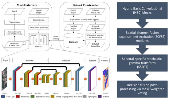
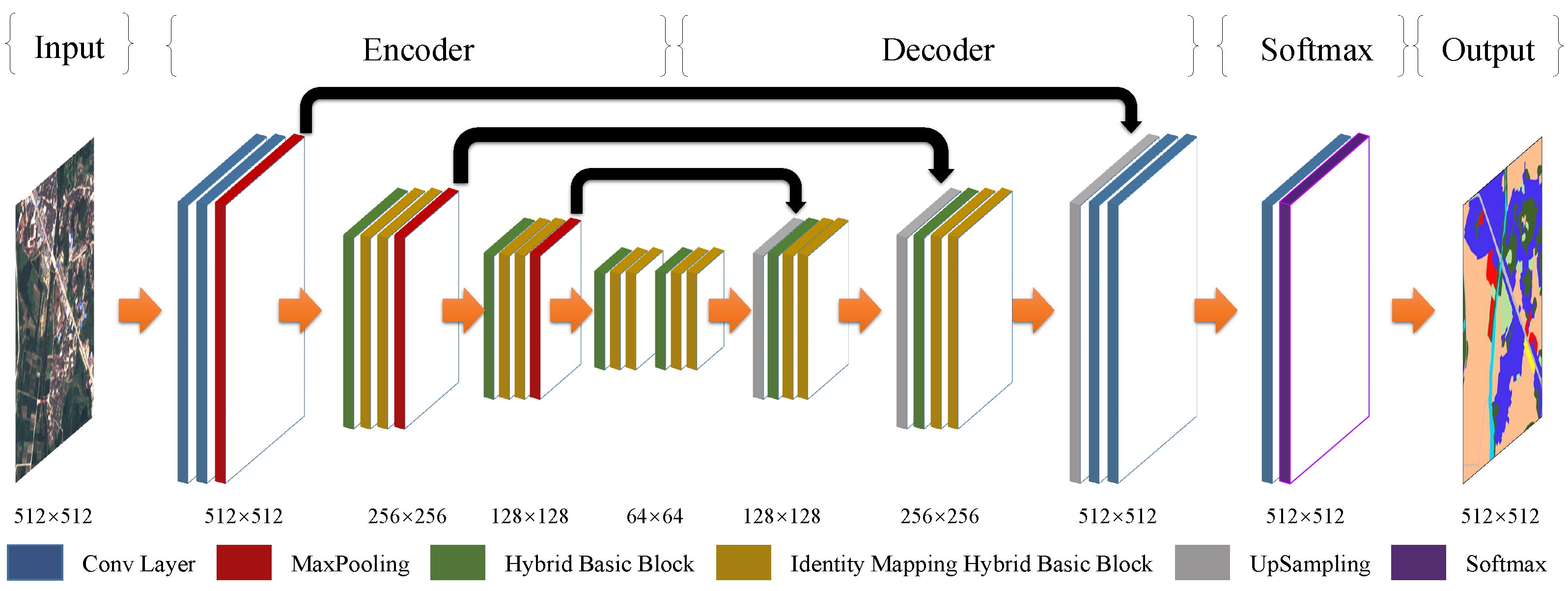
3. SDFCNv2 Architecture

In this section, we introduce the SDFCNv2 framework, which is an improved version of the previously proposed SDFCNv1 framework. Our SDFCNv2 framework includes hybrid basic convolutional blocks to enlarge receptive field, new-designed Squeeze-and-Excitation modules for feature recalibration, a spectral-specific stochastic gamma transform-based (SSSGT-based) data augmentation method, and a decision fusion procedure through mask-weighted voting.

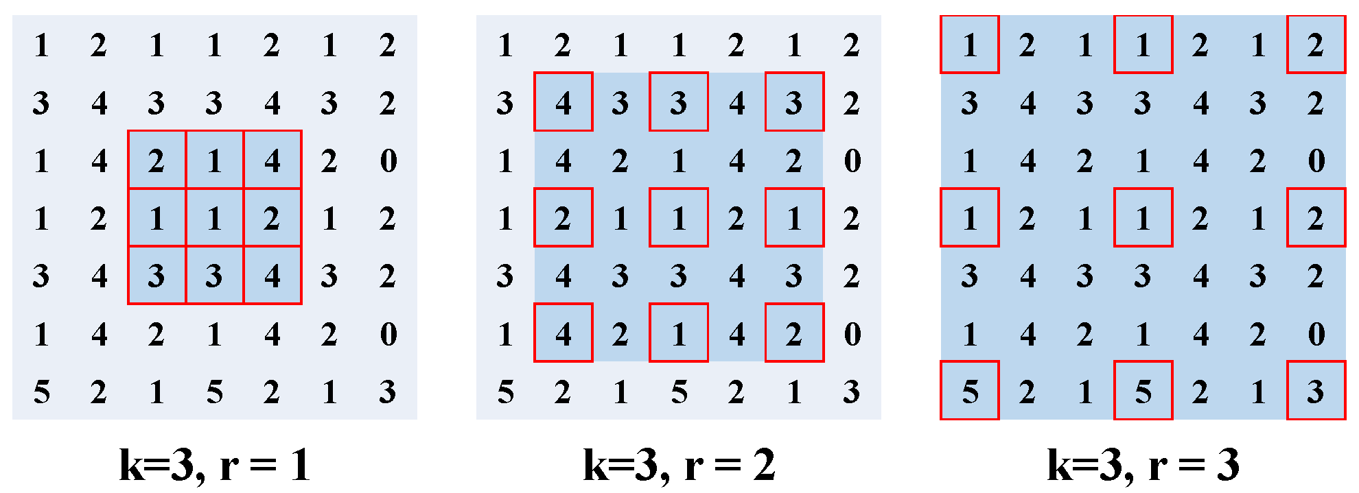
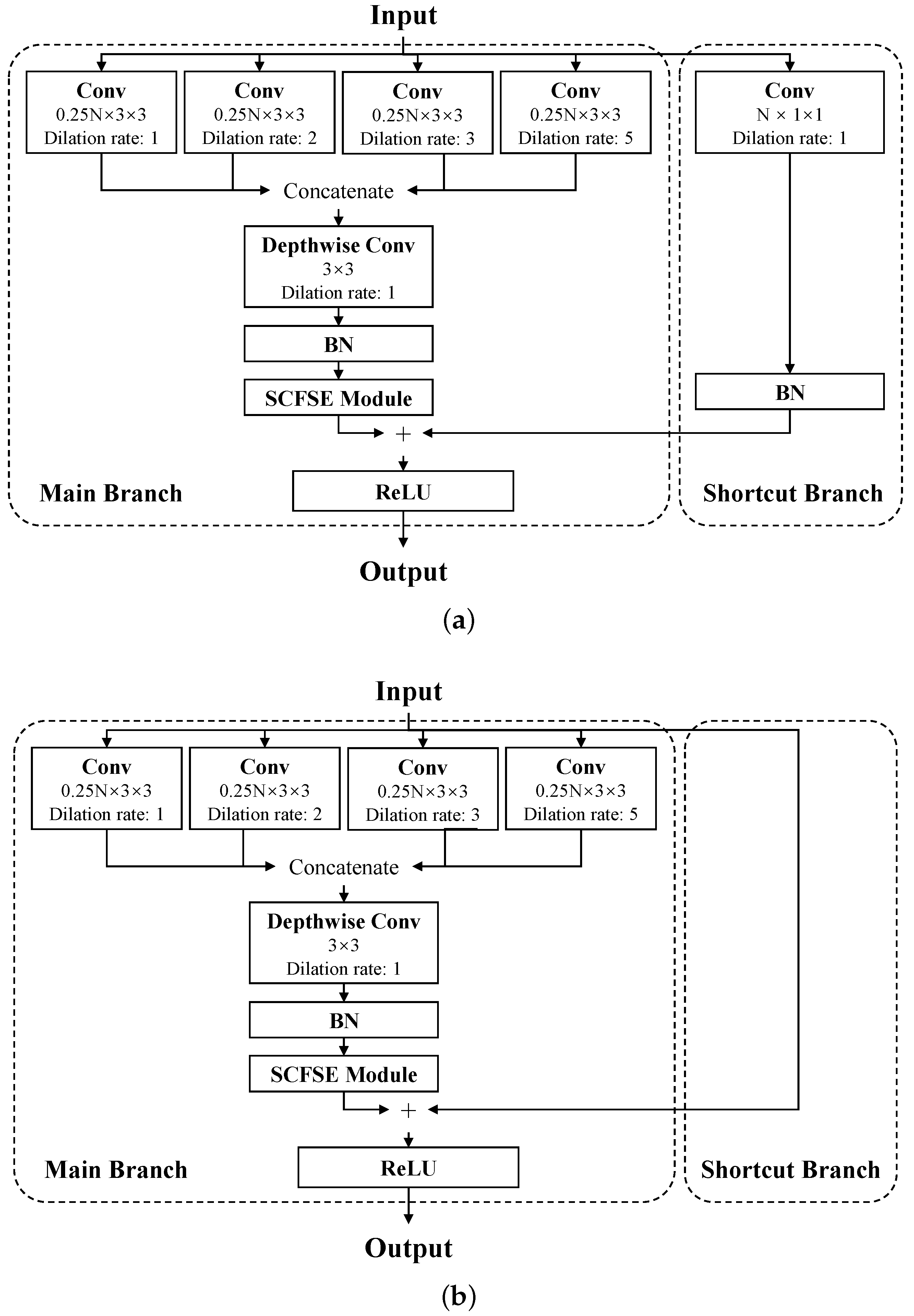
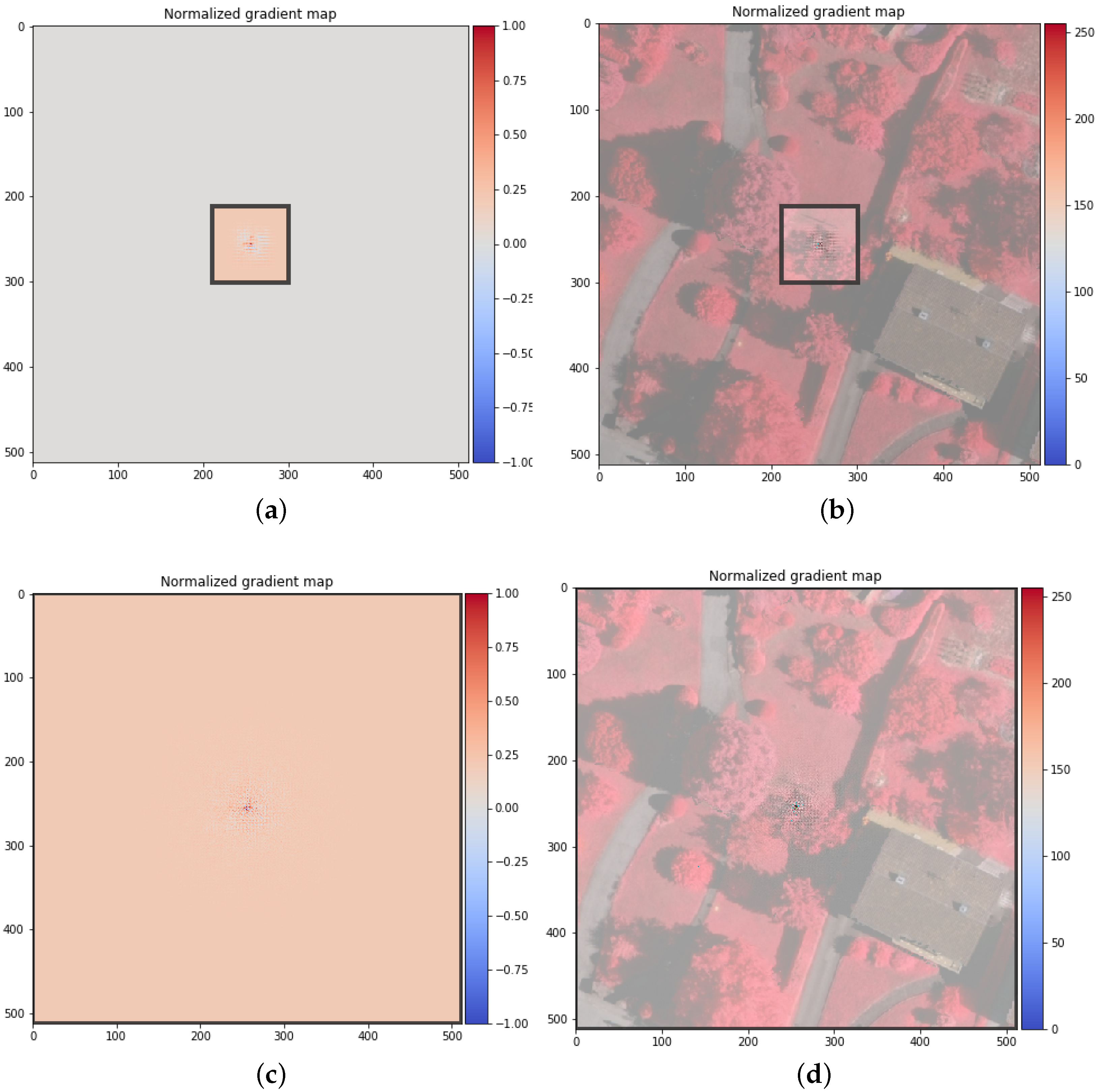
3.1. Hybrid Basic Convolutional (HBC) Block

In general, the model in our proposed framework shares a similar architecture with SDFCNv1, as shown in Figure 3. The structural difference between SDFCNv1 and SDFCNv2 first lies in the basic convolutional blocks.

The encoder and decoder of the FCN model are usually stacked by multiple basic blocks. Each basic block consists of one or more convolutional layers, Batch Normalization (BN) layers, and an activation layer. The pooling layers are distributed between the basic blocks, enabling the model to extract multi-scale features.

In our SDFCNv2 model, following the principles of reducing parameters and expanding receptive field, we design a hybrid basic convolutional (HBC) block with dilated convolutional layers and a depthwise convolutional layer. Figure 4a denotes the structure of the HBC block. The HBC block in SDFCNv2 contains a main branch (the dashed box on the left of the Figure 4a) and a shortcut branch (the dashed box on the right of the Figure 4a). The main branch of the HBC block first splits input feature maps into four small branches by four dilated convolutional layers with different dilated rates of 1, 2, 3, and 5, which can eliminate gridding effect caused by accumulatively adopting dilation layers with single rate in a model [44]. Then, four branches are concatenated and sent to a depthwise convolutional layer. The main branch can be written in form of a function $HB{C}_{main}(·)$ as follows:

$$HB{C}_{main}\left(x\right)=BN(\sum _{i\in \{1,2,3,5\}}D{C}_{3\times 3}(Con{v}_{3\times 3}^i(x,W_1),W_2)))$$

(2)

where x is the input feature map, $D{C}_{3\times 3}(·)$ denotes a depthwise convolution operator with a window size of $3\times 3$, $Con{v}_{3\times 3}^i(·)$ denotes a dilated convolution with a dilated rate of i, $W_1$ and $W_2$ indicate weights to be trained, and $BN$ means the batch normalization process. The shortcut branch in HBC blocks can be represented by $HB{C}_{shortcut}(·)$:

$$HB{C}_{shortcut}\left(x\right)=BN\left(Con{v}_{1\times 1}(x,W_0)\right)$$

(3)

where $Con{v}_{1\times 1}(·)$ denotes a convolution operator with a window size of $1\times 1$ and $W_0$ denotes the weight parameters. The output of one HBC block can be denoted as $HBC(·)$:

$$HBC\left(x\right)=Relu(HB{C}_{main}\left(x\right)+HB{C}_{shortcut}\left(x\right))$$

(4)

where $Relu\left(x\right)=max(x,0)$.

Multiple HBC blocks with identity mapping as a shortcut branch (called identity mapping basic blocks, IMHBC) can be stacked to make model deeper. The authors of [57] proved that identity mapping will not cause the gradient to vanish. The function of shortcut branch of the identity mapping basic block $IMHB{C}_{shortcut}(·)$ is as follows:

$$IMHB{C}_{shortcut}\left(x\right)=x$$

(5)

Similarly, the output of one IMHBC block can be represented by $IMHBC(·)$:

$$IMHBC\left(x\right)=Relu(HB{C}_{main}\left(x\right)+IMHB{C}_{shortcut}\left(x\right))$$

(6)

Consequently, there are two or three identity mapping basic blocks after each HBC block in one block group $Group\left(x\right)$, as shown in Figure 3.

$$Group\left(x\right)=MaxPooling\left(IMHBC\right(IMHBC\left(HBC\right(x\left)\right)\left)\right)$$

(7)

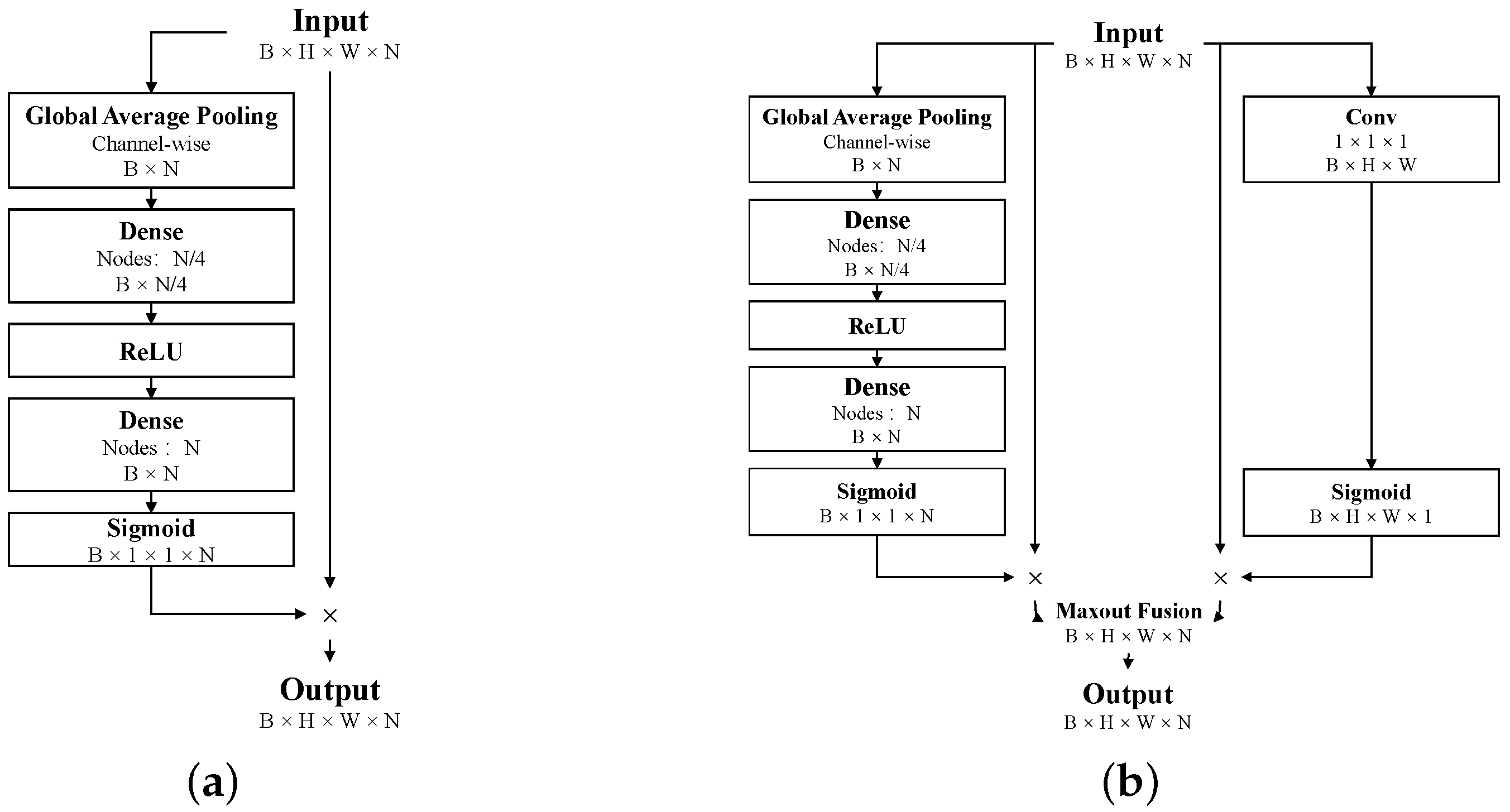
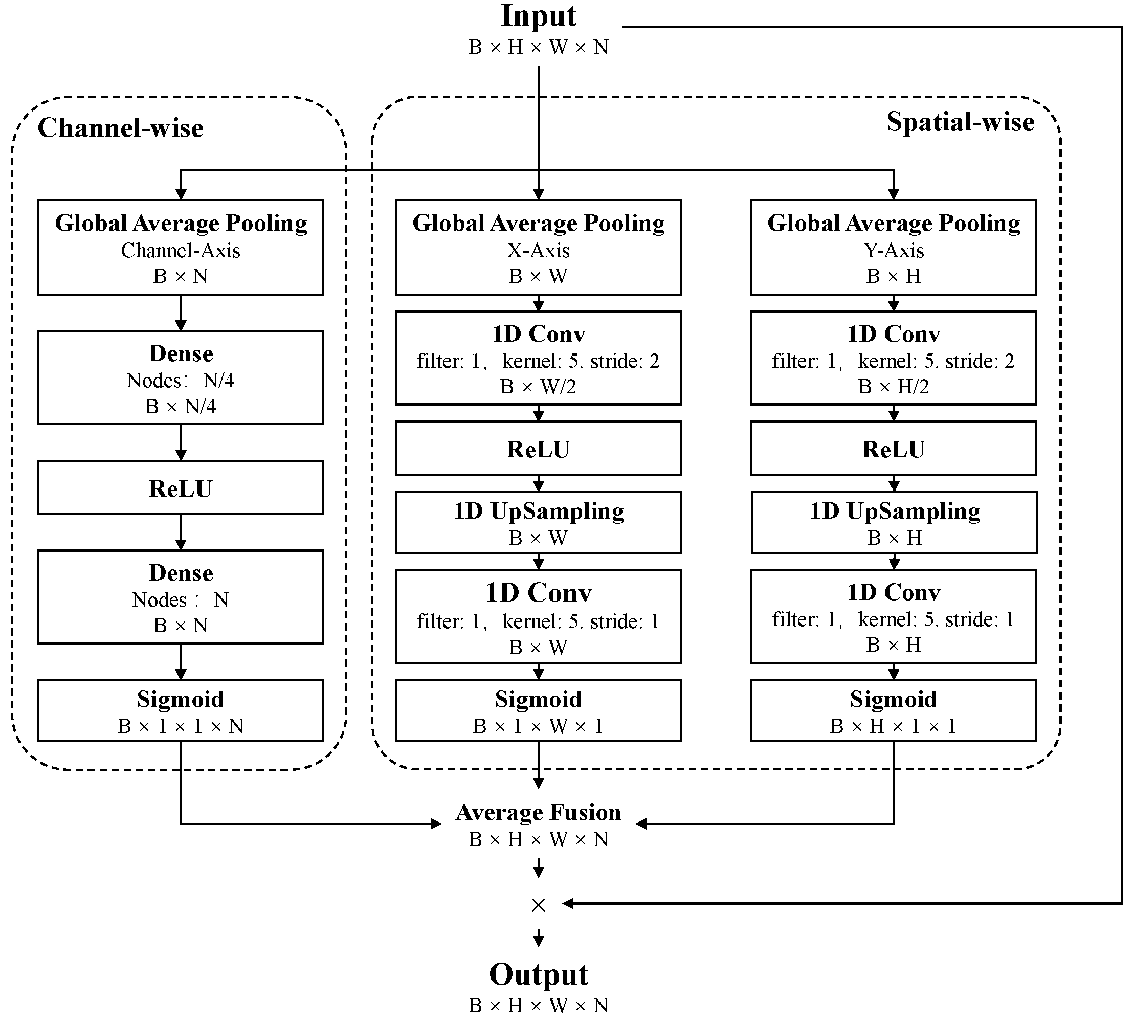
3.2. Spatial and Channel Fusion Squeeze-and-Excitation (SCFSE) Module

To improve the performance of the HBC block, we further propose an attention-based spatial and channel fusion Squeeze-and-Excitation (SCFSE) module to recalibrate feature maps in terms of channel and space. Figure 5 presents the structure of SCFSE module, which contains three branches. We suppose the input data of the SCFSE module has a size of $B\times W\times H\times N$. The left branch (denoted as the Channel-wise branch in Figure 5) has the same function as the SE block [53], and is used to recalibrate feature maps in a channel-wise manner and generate the weight of each channel. Unlike the scSE block [54], the two branches on the right side of the SCFSE module (denoted as the Spatial-wise branches in Figure 5) are used to recalibrate features on the X-axis (the horizontal axis) and Y-axis (the vertical axis). Considering to take full advantage of adjacency, a 1-D convolution operator is used instead of the fully connected (Dense) layer. The three branches are merged through an average fusion process, and the final output of the SCFSE module is obtained by multiplying the original input data by element.

By inserting an SCFSE module in the main branch of the HBC block, the utilization of different filters of the SDFCNv2 model can be improved, at the cost of adding a small number of parameters. As shown in Table 1, the size of the SDFCNv2 model is almost half the size of the SDFCNv1 model, while the SCFSE module only adds 5.5% of additional parameters.

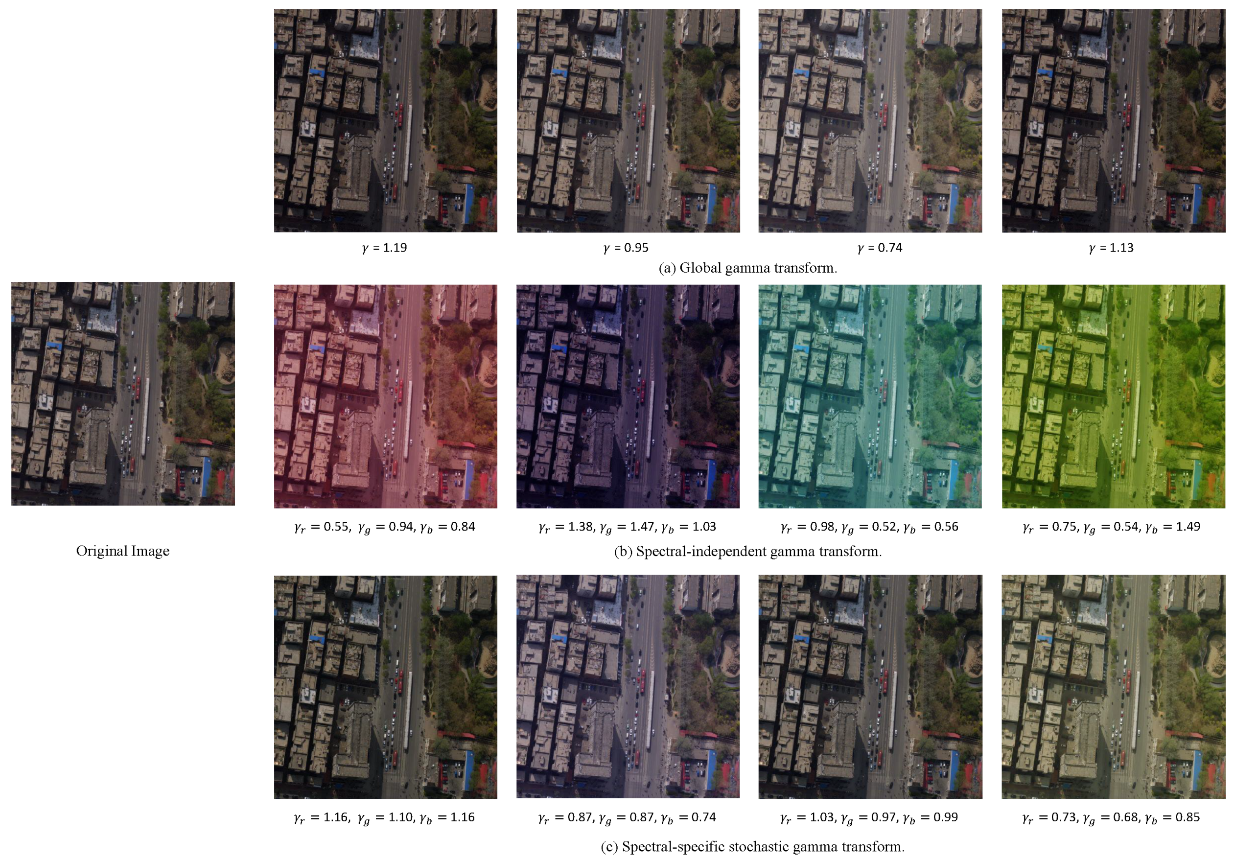
3.3. Spectral-Specific Stochastic-Gamma-Transform-Based Data Augmentation

In SDFCNv1 framework, we adopt three data augmentation methods:

• Random scaling in the range of [1, 1.2];
• Random translation by [−5, 5] pixels;
• Random vertically and horizontally flipping.

However, these three methods only focus on geometry transformations. Facing with seasonal changes, diverse image resolution, and illumination conditions, etc., it may cause significant differences in RS images and affect the model training process. In this section, we conduct a new data augmentation method for multi-spectral images, called spectral-specific stochastic gamma transform (SSSGT), which aims to simulate real multi-source data owing to limited training samples and avoid models overfitting.

Gamma transform is a common nonlinear operation used to adjust the luminance in a video or image system, and is defined as follows:

$$V_{out}=A{V}_{in}^{\gamma }$$

(8)

where input value $V_{in}$ is raised to the power $\gamma$ and multiplied by the constant A to acquire the output value $V_{out}$. Usually, A is set to 1, the input and output value are both in range of [0, 1].

Global gamma transform (GGT) is one of the popular data augmentation methods. All spectral bands of an image are processed by gamma transform with $A=1$ and a global-wise random value $\gamma$, which obeys the uniform distribution of [0.5, 1.5]. Figure 6a shows four examples processed by GGT. Augmented images only reveal their changes in image luminance and contrast.

A variant of GGT method is the spectral-independent gamma transform (SIGT), in which the $\gamma$ values of each band are uniformly distributed independently of each other. From four examples in Figure 6b, the SIGT method tends to generate images with larger color shifts, which are difficult to appear in real scenes.

In order to overcome the drawbacks of the above two methods, we propose a Spectral-specific stochastic-gamma-transform (SSSGT) method. In this method, we first define a global random variable ${\gamma }_{global}$ as the base value, obeying a uniform distribution $U[0.5,1.5]$, namely, ${\gamma }_{global}\sim U[0.5,1.5]$. We suppose that the i-th spectral band has its own disturbance random value ${\gamma }_i^D$ and ${\gamma }_i^D\sim U[-0.2,0.2]$. The final gamma value for the i-th spectral band ${\gamma }_i$ is then defined as follows:

$${\gamma }_i={\gamma }_{global}+{\gamma }_i^D$$

(9)

Four examples of our proposed method are listed in Figure 6c. Our SSSGT method is able to synthesize more kinds of hue transformation than GGT method and is closer to the real multi-source data situation than SIGT method.

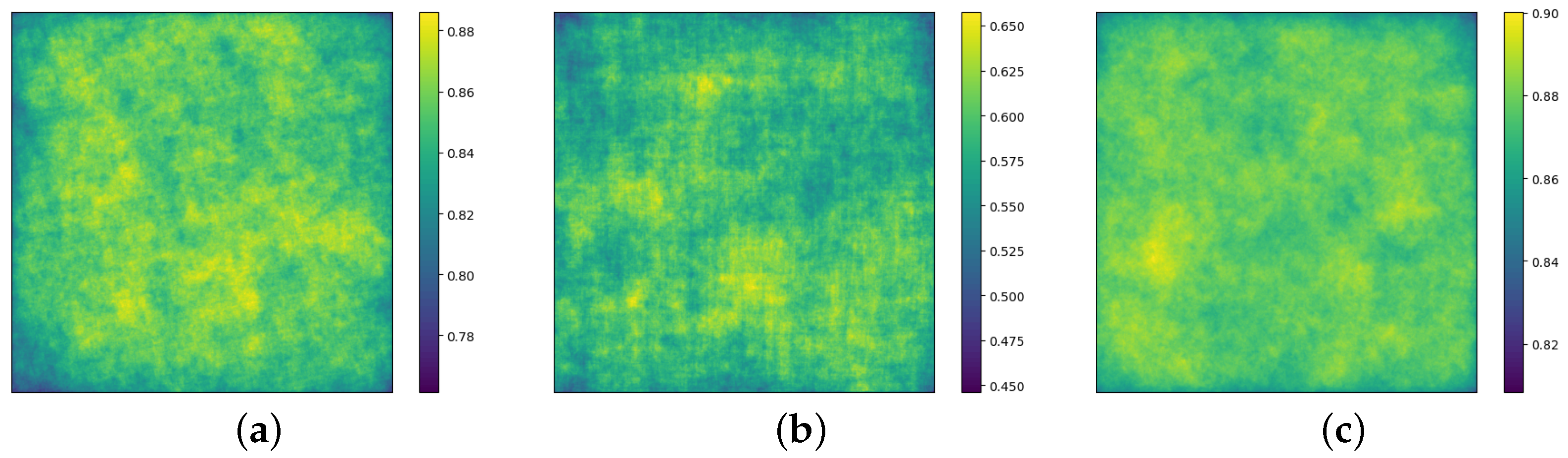
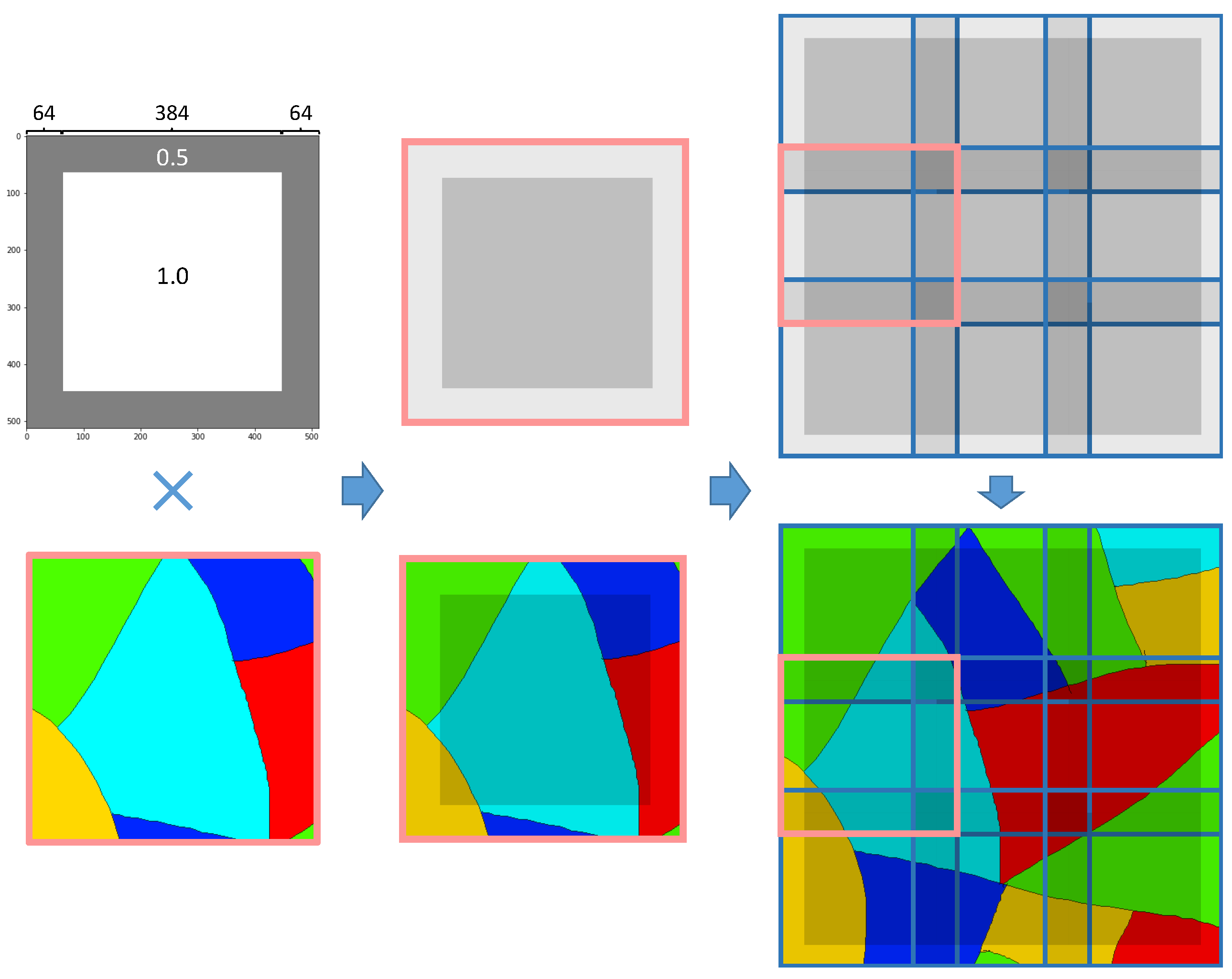
3.4. Decision Fusion Postprocessing via Mask-Weighted Voting

In order to realize the prediction of the overlarge RS image, many methods adopt the overlay fusion prediction strategy with majority voting in the sliding-window mode to postprocess the model prediction results. They simply merge the patch predictions and average the predictions of the overlapping regions to obtain the final predictions of the overlarge images. However, there is an inherent contradiction between the accuracy of this method and the amount of calculation caused by the increase of the degree of overlap of the sliding window [31]. Specifically, a small overlap may lead to discontinuous block effects in the final prediction result, while a large overlap will obtain higher prediction accuracy but increase the amount of calculation exponentially. Therefore, this paper attempts to propose a new postprocessing method to solve this contradiction, which not only reduces the calculation amount, but also improves the prediction accuracy.

In FCN models, a zero-padding operation is commonly applied to the marginal area of feature map during convolutional or pooling operations to ensure that the input and output feature maps are of the same size or have multiple relationship. However, the theoretical receptive field of the marginal pixels of the input feature map is smaller than that of the center pixels. The prediction accuracy of the network model for the middle region of the input image is higher than that of the marginal region, resulting in the above-mentioned block effect. In order to further analyze the difference in the spatial distribution of the accuracy of the FCN model at different pixel positions of the input image, we conduct statistics on the spatial distribution of the sample prediction accuracy in the test sets of the Potsdam, Evlab, and Songxi datasets. The input sample size of the model is $512\times 512$ pixels, and the accuracy distribution results are shown in Figure 7. According to the accuracy distributions on the three datasets, the prediction accuracies of pixels around the four corners and marginal area are lower than that of the pixels in the middle region.

Inspired by the spatial distribution difference of the accuracy of the FCN model, we propose an improved postprocessing methods called mask-weighted voting decision fusion. As shown in Figure 8, we first initialize a mask with the same size as the model input. Taking $512\times 512$ pixels as the model input size, we set the weight for the middle region ($384\times 384$ pixels) to 1, and the weight of the marginal area of the mask to 0.5. We then multiply the patch-wise predictions with the constructed weighted-mask, and merge the multiplied results into the overlay fusion strategy. Compared with the classic overlay fusion strategy, it can effectively suppress the weight of the result of the marginal area, while the calculation amount of the model prediction remains similar.

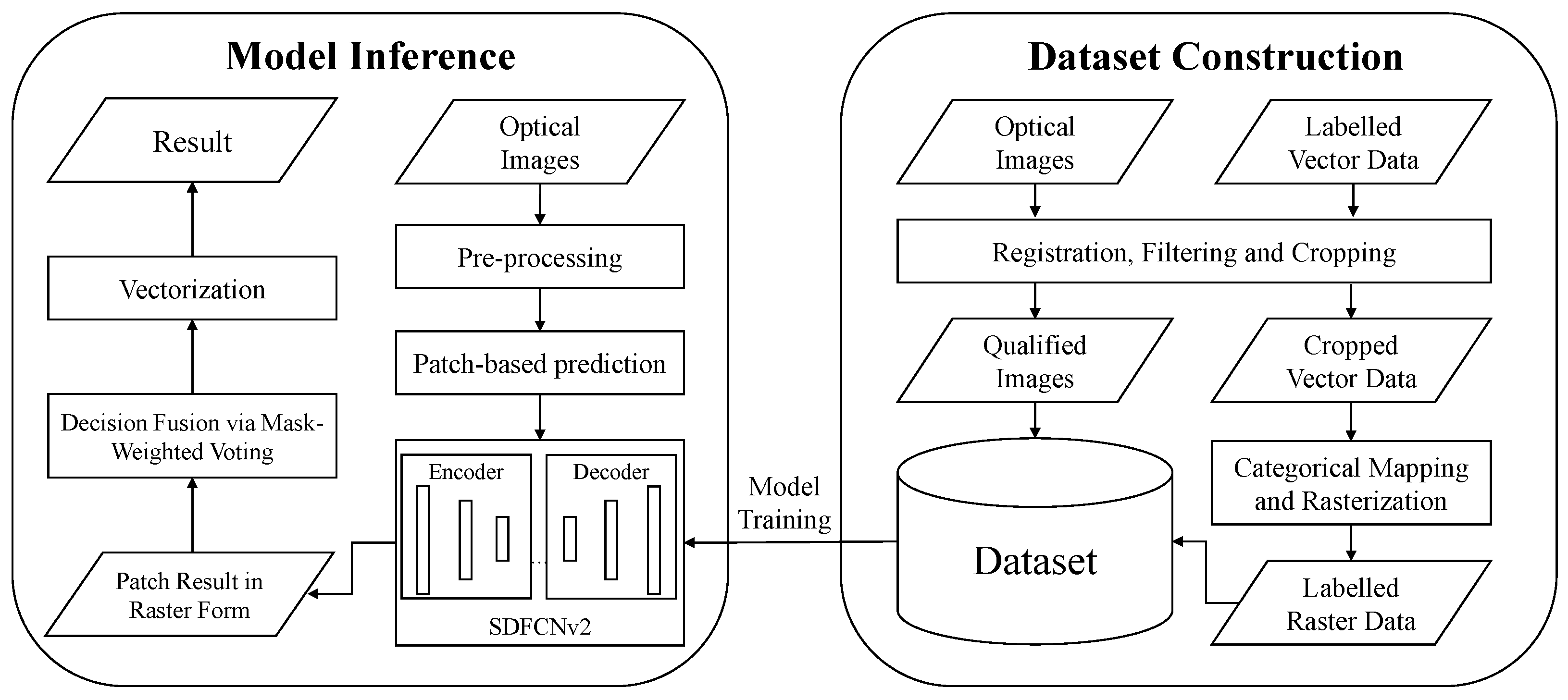
4. Dataset Construction and the Whole Framework

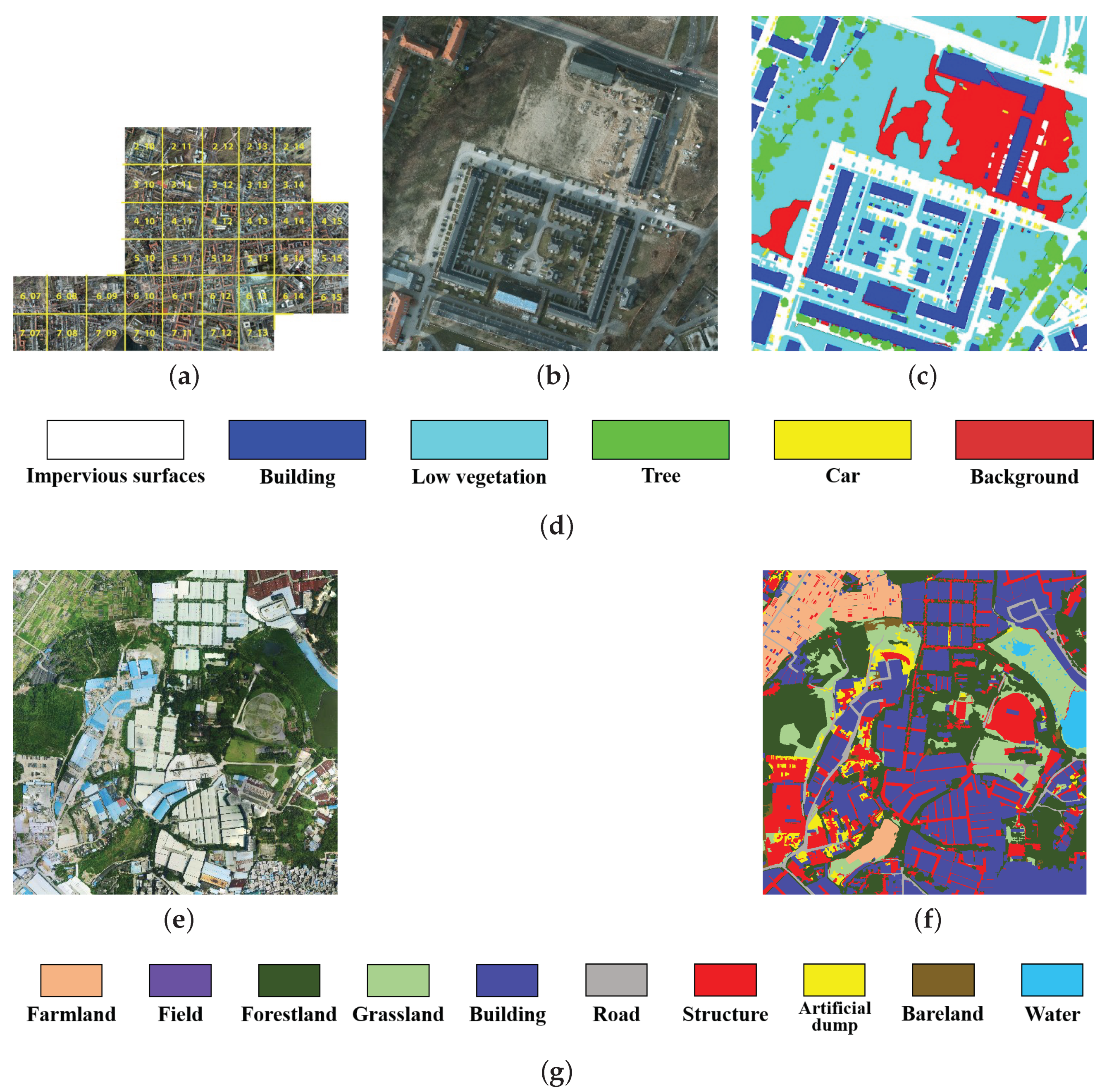
4.1. Dataset Construction

To evaluate our proposed framework, we construct a novel large-scale dataset from our collected real land-cover mapping data. The land-cover data we collected is full-covered polygon data from the Chinese Geographic Condition Survey and Mapping Project (CGCSMP) with categorical information, which cannot be directly used for FCN model’s training. Acquired with a series of optical RS images and the corresponding full-covered vector data in the same region, we design an automatic process to effectively generate datasets suitable for model training. The processing flow is listed as follows:

1.

Data registration. RS images are first aligned with the corresponding label vector data in the identical coordinate system. For optical RS images, we need to further unify their spatial resolution, radiometric resolution and image spectral bands. In this paper, we convert all RS images into 8-bit raster data with a spatial resolution of 0.5 m, containing three spectral bands of red, green, and blue. Besides, we crop the vector data according to the rectangular area of the RS raster data, and we need to filter out the partly overlapping area.

2.

Categorical mapping. We extract the attributes of the category codes from the cropped vector data, convert them into category labels and encode them. (For example we encode ten categories from 0 to 9).

3.

Rasterization. We rasterize the cropped vector data according to the spatial resolution of the RS images and generate labeled raster data, where each pixel value represents a specific category code.

4.

Invalid label cleaning. In full-covered label vector data, invalid labels due to incomplete coverage, edge connection errors, and label errors may appear with extremely low probability. Therefore, it is necessary to classify invalid labels into a certain category for cleaning up.

5.

Data partition. The image–label pairs are divided into training set, validation set, and test set according to the designed proportion.

6.

Generating metadata. In accordance with the partitioned dataset, we need to record the dataset name, partition results, basic attributes of images, categories, file naming rules as metadata to facilitate dataset management and model training.

7.

Manual verification. Check the generated dataset to avoid problems in the above process.

In this paper, we collected a series of optical digital orthophoto maps (DOMs) and corresponding full-covered label vector data in Songxi County, Fujian Province, China. The administrative area of Songxi County is approximately 1043 square kilometers. According to the CGCSMP specification, the DOMs and the corresponding vector data in 10 land cover categories are shown in Figure 9. There are 58 DOMs in Songxi region, collected from different sources including aerial images, Pleiades satellite RS images, and QuickBird satellite RS images. The average image size is $12900\times 9800$ pixels. All DOMs are reprojected to the same coordinate system and resampled to the same 0.5 m spatial resolution.

We then follow the above process to automatically construct the Songxi dataset. The number of eligible DOMs (the boundaries of which are completely within the range of the vector data) is 26. We divide the constructed image-label pairs into training set (12 DOMs), validation set (5 DOMs), and test set (9 DOMs).

4.2. The Whole Sdfcnv2 Framework

Our entire RSIA semantic segmentation framework consists of dataset construction, model training, and inference, as shown in Figure 10. Combining a series of optical RS images and labeled vector data, the dataset construction process is able to automatically generate a large-scale sample dataset suitable for FCN model training. After using the improved SDFCNv2 model to train the constructed dataset, we use the trained model to predict test images, and merge the patch predictions with the decision fusion through mask weighted voting. Finally, a vectorization process is conducted on entire raster prediction to generate vector data and each object contains a category code.

5. Experimental Results and Analysis

5.1. Experiment Datasets

In this section, we conducted experiments on two public datasets (Potsdam dataset [33], Evlab dataset [58]) and one constructed dataset (Songxi dataset).

The Potsdam dataset is provided by the International Society for Photogrammetry and Remote Sensing (ISPRS), and consists of DOMs generated from aerial images of Germany. The ground sample distance (GSD) is 0.05 m. The DOMs contain four spectral bands of infrared (IR), red (R), green (G), and blue (B). The corresponding pixel-wise labels contains six categories: impervious surfaces, building, low vegetation, tree, car, and background. The Potsdam dataset contains 38 image tiles, which are divided into training set (18 tiles with ID 2_10, 2_11, 3_10, 3_11, 4_10, 4_11, 5_10, 5_11, 6_7, 6_8, 6_9, 6_10, 6_11, 7_7, 7_8, 7_9, 7_10, and 7_11), validation (val) set (six tiles with ID 2_12, 3_12, 4_12, 5_12, 6_12, and 7_12) and test set (14 tiles with ID 2_13, 2_14, 3_13, 3_14, 4_13, 4_14, 4_15, 5_13, 5_14, 5_15, 6_13, 6_14, 6_15, and 7_13). Image series, example image, ground truth label of ID 2_10, and dataset legend are shown from Figure 11a,d.

The Evlab dataset consists of 45 DOMs acquired from WorldView-2, GeoEye, QuickBird, GF-2, and aircrafts. The average size of each DOM is $4500\times 4500$ pixels, and the GSD ranges from 0.1 m to 1 m. Pixel-wise labels contain ten categories: farmland, field, forestland, grassland, building, road, structure, artificial dump, bareland, and water. We randomly divide 45 image tiles into training set (28 tiles with ID 1, 4, 7, 10, 11, 12, 13, 14, 15, 16, 19, 21, 22, 23, 26, 29, 31, 32, 33, 35, 36, 37, 38, 40, 42, 43, 44, and 45), validation set (nine tiles with ID 2, 5, 8, 17, 20, 24, 27, 30, and 39) and test set (eight tiles with ID 3, 6, 9, 18, 25, 28, 34, and 41). Example image, ground truth label of ID 10, and dataset legend are shown from Figure 11e–g.

The third dataset is our constructed Songxi dataset, which has been introduced in Section 4.1. Besides, the labels share the same categories as the Evlab dataset. In all, we summarize the information of each experiment dataset in

Table 2. General information of experiment dataset.

Dataset	Source	GSD	Spectral Band	Category	Number of Image and Division (Train, Val and Test)
Potsdam	Aerial	0.05 m	IRRGB	6	38 (18, 6, 14)
Evlab	Satellite & Aerial	0.1–1 m	RGB	10	45 (28, 9, 8)
Songxi	Satellite & Aerial	0.5 m	RGB	10	26 (12, 5, 9)

.

5.2. Model Implementation

All FCN models in our experiments are trained using the back-propagation algorithm, and the minibatch size is 2. Adam is adopted as the weight-updating optimization algorithm [59]. The learning rate is set to 0.01, and the weight decay rate of L2-loss is set to 0.0005. In the Potsdam dataset, the model input size is $512\times 512\times 4$, and the number of predicted categories is 6. In Evlab and Songxi dataset, the model input size is $512\times 512\times 3$, and the number of predicted categories is 10. Moreover, each FCN model is trained for 60 epochs in the Potsdam dataset, 50 epochs in the Evlab dataset, and 40 epochs in the Songxi dataset.

Pixel overall accuracy (OA), kappa coefficient (K, Kappa) [60], and mean intersection over union (mIoU) are adopted as accuracy assessment metrics. We calculate the accuracy metrics in the pixel prediction results represented by one pixel value, rather than in the prediction result represented by three pixel values adopted in ISPRS 2D semantic segmentation contest [33]. The loss function utilized in the training process is a combination of the categorical cross-entropy function and the Lovasz–Softmax function [61] to optimize the OA and mIoU metrics at the same time. During the training and validation process, the trained models of each epoch will be validated on the validation set. The validation loss (val_loss) of each epoch will be recorded, and the checkpoint that reaches the lowest val_loss will be used to evaluate the final accuracy on the test set.

All experiments are conducted on a supercomputing system with Intel(R) Xeon(R) E5-2640 v4, 128 GB RAM and NVIDIA Tesla V100 (16,384 MB memory). We implement our framework based on TensorFlow 2.3.

In our SDFCNv2 framework, we adopt the following augmentation methods during training process:

• Random rotation by 0°, 90°, 180° or 270°;
• Random vertically and horizontally flipping;
• Random offset (Maximum offset range is consistent with the model input patch size.);
• Selective gamma-transform-based augmentation methods, including GGT, SIGT and SSSGT.

In model prediction (testing or inference) process, following strategies are selectively and experimentally adopted:

• Overlap fusion strategy with majority voting.
• Mask-weighted voting decision fusion.
• Rotation by four kinds of degrees (0°, 90°, 180° or 270°).

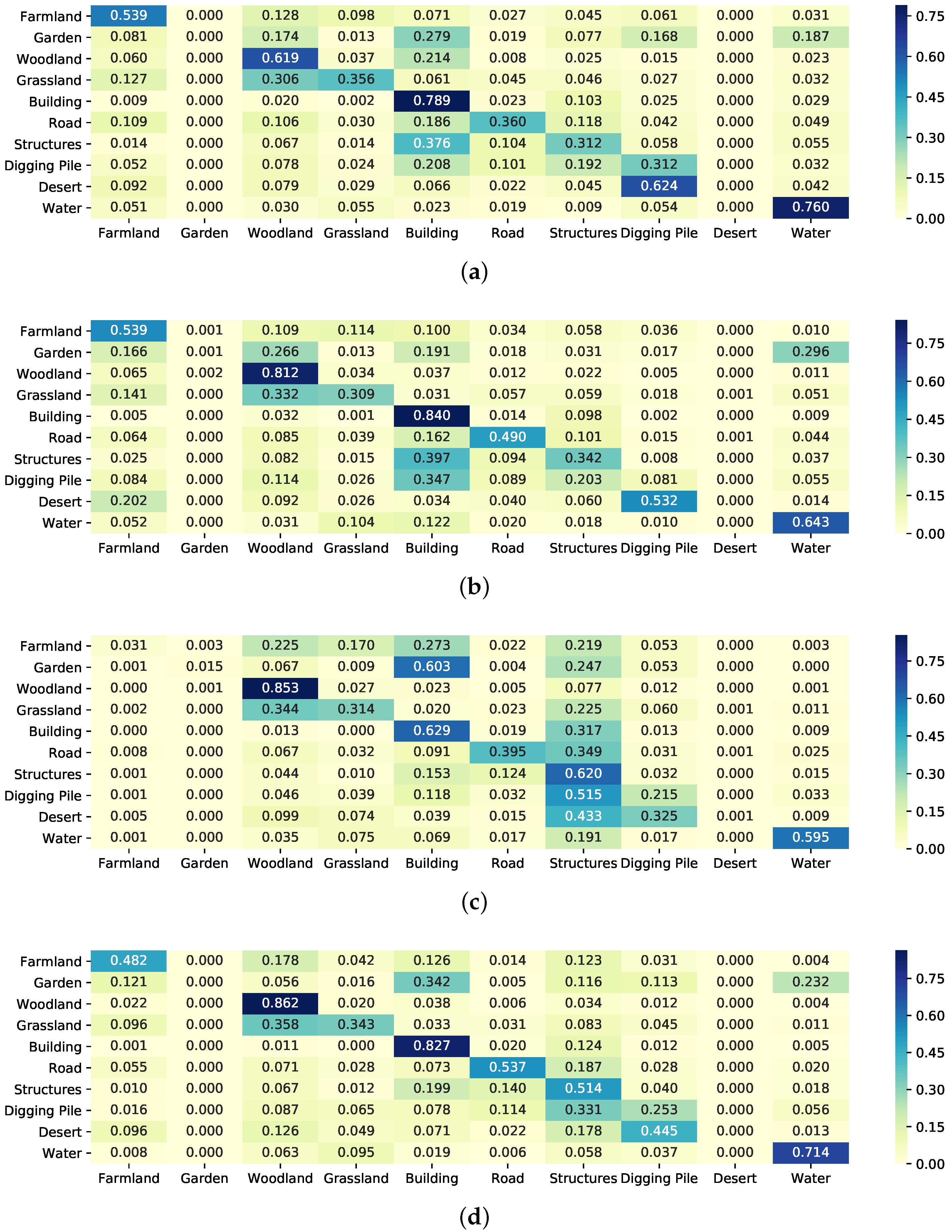
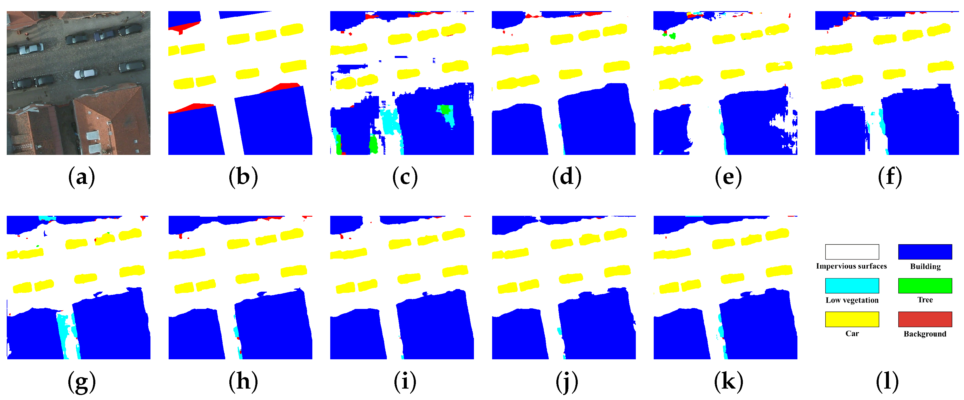
5.3. Experiments on Model Structures and Different Feature Recalibration Modules

In this section, we first implemented the experiments of four classic FCN models, including FCN-8s, PSPNet, Deeplab v3+, and HRNet V2, as well as our previously proposed SDFCNv1, to evaluate the performance of our SDFCNv2 model. In addition, we have equipped the SDFCNv2 model with different feature recalibration modules in our HBC block (see Figure 4a), including the SE module [53], the scSE module [54], and the designed SCFSE module. The experimental results on the three datasets are listed in

Table 3. Performances of different models and SE modules on three experiment datasets.

Model	Potsdam Dataset			EvLab Dataset			Songxi Dataset
	OA	K	mIoU	OA	K	mIoU	OA	K	mIoU
FCN-8s	0.7444	0.7021	0.5586	0.4730	0.4313	0.2067	0.8567	0.7215	0.3456
PSPNet	0.8059	0.7687	0.6364	0.4956	0.4647	0.2559	0.8602	0.7307	0.3833
Deeplab V3+	0.7436	0.6989	0.5263	0.5492	0.5085	0.2733	0.7708	0.5758	0.2042
HRNet V2	0.8380	0.8029	0.6584	0.5288	0.4831	0.2453	0.8584	0.7208	0.3448
SDFCN V1	0.8006	0.7615	0.6081	0.5083	0.4641	0.2448	0.8627	0.7280	0.3440
SDFCNv2	0.8473	0.8140	0.6741	0.5773	0.5380	0.2963	0.8461	0.6955	0.3458
SDFCNv2+SE	0.8419	0.8077	0.6744	0.5631	0.5301	0.3017	0.8657	0.7340	0.3708
SDFCNv2+scSE	0.8262	0.7920	0.6685	0.4883	0.4532	0.2496	0.8697	0.7471	0.3621
SDFCNv2+SCFSE	0.8503	0.8177	0.6782	0.5945	0.5539	0.3208	0.8762	0.7562	0.3980

.

We first compare SDFCNv2 without feature recalibration modules with SDFCNv1 to evaluate the performance improvement that our proposed HBC block can bring. From the results listed in Table 3, we found that the OA, Kappa, and mIoU values can be significantly increased by 4.67%, 5.25%, and 6.6% in the Potsdam dataset and by 6.9%, 7.39%, and 5.15% in the Evlab dataset, while the OA and Kappa values decrease by 1.66% and 3.25% and the mIoU value is only 0.18% higher in the Songxi dataset. Note that the number of parameters of SDFCNv2 is less than half of that of SDFCNv1. In addition, we normalize and visualize the gradients of the input feature map of Softmax layer in back propagation corresponding to the center point of the input image to analyze the receptive fields of SDFCNv1 and SDFCNv2. Figure 12 shows the receptive fields at the center of $512\times 512$ input image. It can be seen that the receptive field of the SDFCNv2 model is significantly larger than that of the SDFCNv1, covering the entire input image, which helps the model capture semantic information and improve segmentation accuracy.

We further analyze the results of SDFCNv2 model equipped with different feature recalibration modules. It can be seen that SDFCNv2 model with SE modules brings 0.03%, 0.54% and 2.5% improvements of mIoU in Potsdam, Evlab and Songxi datasets. The performances of the model with scSE modules suffer an obvious decrease of 0.56% and 4.67% in mIoU for Potsdam and Evlab datasets, but improve 1.63% in mIoU for Songxi dataset. In contrast, the proposed SCFSE module can bring remarkable improvement in SDFCNv2 model compared to SE and scSE modules. It can be observed the model with SCFSE modules brings 0.41%, 2.45% and 5.22% improvement in mIoU for three datasets, which indicates our SCFSE module can further improve the representation capability of the network.

To prove the effectiveness of our SCFCNv2 model, we compare our method with four commonly-used methods, as listed in Table 3. It can be seen that the performances of SDFCNv2 without feature recalibration modules are slightly superior to other models in the Potsdam and Evlab datasets, but it is not as good as the PSPNet model in the Songxi dataset. Considering the size of SDFCNv2 model is less than half of the PSPNet (as shown in Table 1), the SDFCNv2 model still has a competitive lead. After applying the SCFSE module, SDFCNv2 model outperforms other models by a large margin in all three datasets. Specifically, the mIoU values of SDFCNv2 model with SCFSE modules are 1.98%, 4.75%, and 1.47% higher than the best model among the four commonly used models in Potsdam, Evlab, and Songxi datasets, respectively. Besides, we visualize the normalized confusion matrix results of SDFCNv2, SDFCNv1, and two better-performing common models (i.e., the PSPNet and HRNetV2 models of the Potsdam dataset, the PSPNet and Deeplab v3+ models of the Evlab dataset, and FCN-8s and PSPNet models of the Songxi dataset). Figure 13 shows that the SDFCNv2 model is superior to other models in the classification of buildings, low vegetation, and trees on the Potsdam dataset. Figure 14 shows that the SDFCNv2 model is superior to other models in the classification of woodlands and roads on the Evlab dataset. Figure 15 shows that the SDFCNv2 model is better than other models in the classification of farmlands, gardens, buildings, and roads. The visual results of cropped images randomly selected from the three datasets are shown in Figure 16, Figure 17 and Figure 18, respectively. It can been seen that our SDFCNv2 models produces visually better segmentation maps than other commonly-used models.

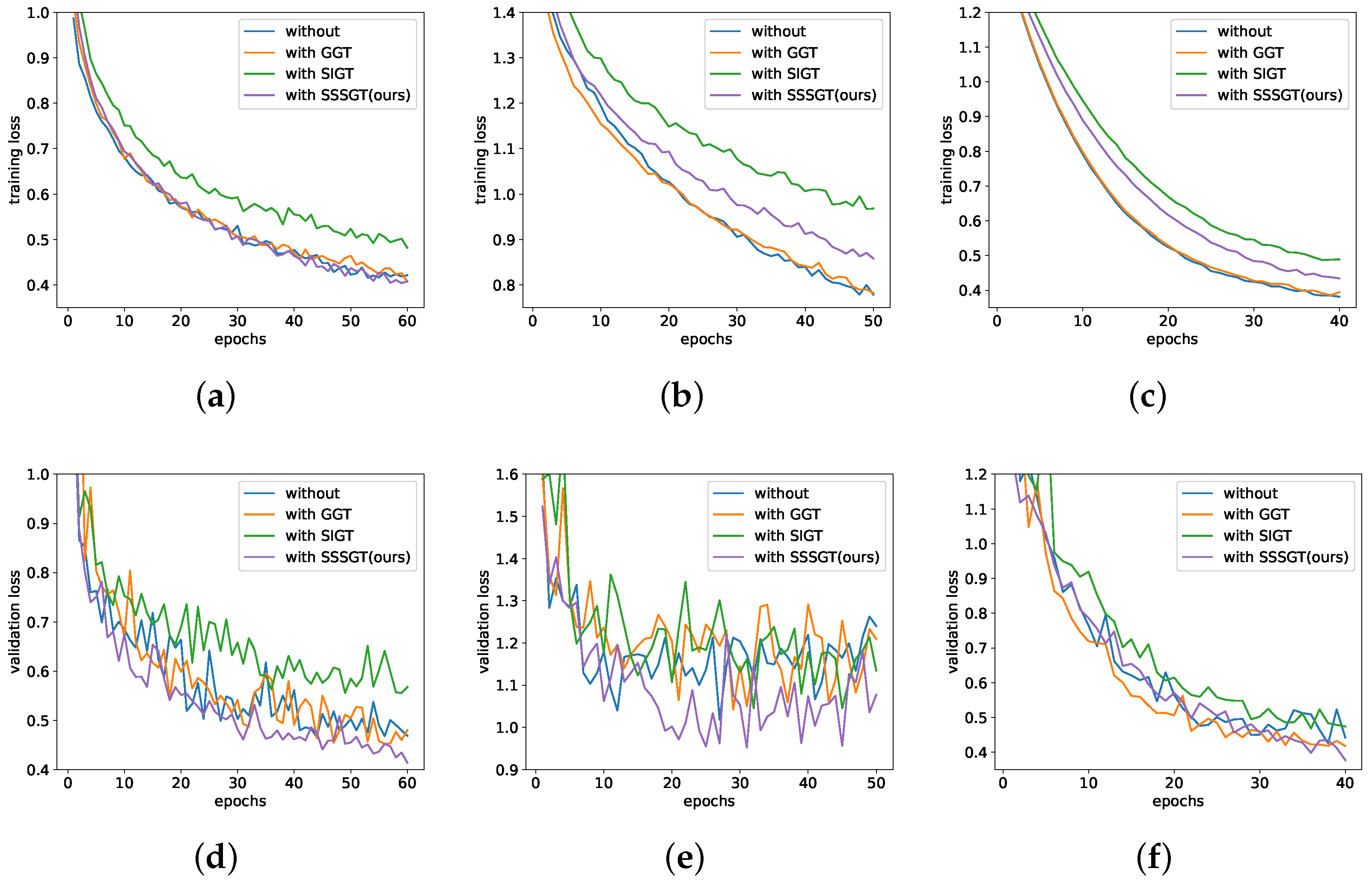
5.4. Experiments on Data Augmentation

Based on the constructed SDFCNv2 model equipped with the SCFSE module, we further tested the effectiveness of different gamma-transform-based data augmentation methods on different datasets. Combining with spatial-transform-based data augmentation, we trained the SDFCNv2 models with GGT augmentation, SIGT augmentation, SSSGT augmentation and without gamma-transform-based augmentation. The experimental results are shown in

Table 4. Performances of different gamma-transform-based data augmentation applied on SDFCNv2 model equipped with SCFSE module in three datasets.

Gamma Augmentation	Potsdam Dataset			EvLab Dataset			Songxi Dataset
	OA	K	mIoU	OA	K	mIoU	OA	K	mIoU
No	0.8306	0.7952	0.6531	0.5398	0.4963	0.2623	0.8501	0.7073	0.3153
GGT	0.8287	0.7927	0.6508	0.4572	0.4263	0.2204	0.8336	0.6714	0.3160
SIGT	0.8261	0.7897	0.6574	0.5181	0.4769	0.2310	0.8718	0.7483	0.3895
SSSGT (ours)	0.8503	0.8177	0.6782	0.5945	0.5539	0.3208	0.8762	0.7562	0.3980

.

Results indicate that, compared with no-gamma-transform-based augmentation, the additional utility of GGT method yet reduces the performance of the model in the Potsdam and Evlab datasets, and the performance in the Songxi dataset is hardly improved. The use of SIGT method slightly increased the mIoU value on the Potsdam dataset, deteriorated the performance on the Evlab dataset, and realized improvement on the Songxi dataset. By contrast, our proposed SSSGT method achieves optimal results among all methods. Specifically, using our SSSGT method brings robust improvements on the Potsdam, Evlab, and Songxi datasets, that is, compared with the no-gamma-transform-based augmentation method, the mIoU values are increased by 2.51%, 5.85%, and 8.27%. Compared with the Potsdam dataset, the Evlab and Songxi datasets consist of images from more diverse sources, which bring more difficulties to model training. Nevertheless, our SSSGT augmentation method can bring obvious improvement especially on these two datasets, which indicates the SSSGT method is able to reasonably simulate the distribution of real image data. Our proposed SSSGT method optimizes the training strategy and successfully improves the generalizability and performance of the model.

Moreover, we plot the training and validation loss curves using different gamma-transform-based augmentation methods on the three datasets in Figure 19. As shown in the plotted loss curves, we can observe that the validation loss curves of the proposed SSSGT are clearly lower than other augmentation methods during training process. Effective accuracy metrics of SSSGT listed in Table 4 verify that SSSGT augmentation method helps prevent overfitting phenomenon and improve model performance.

5.5. Experiments on Decision Fusion via Mask-Weighted Voting

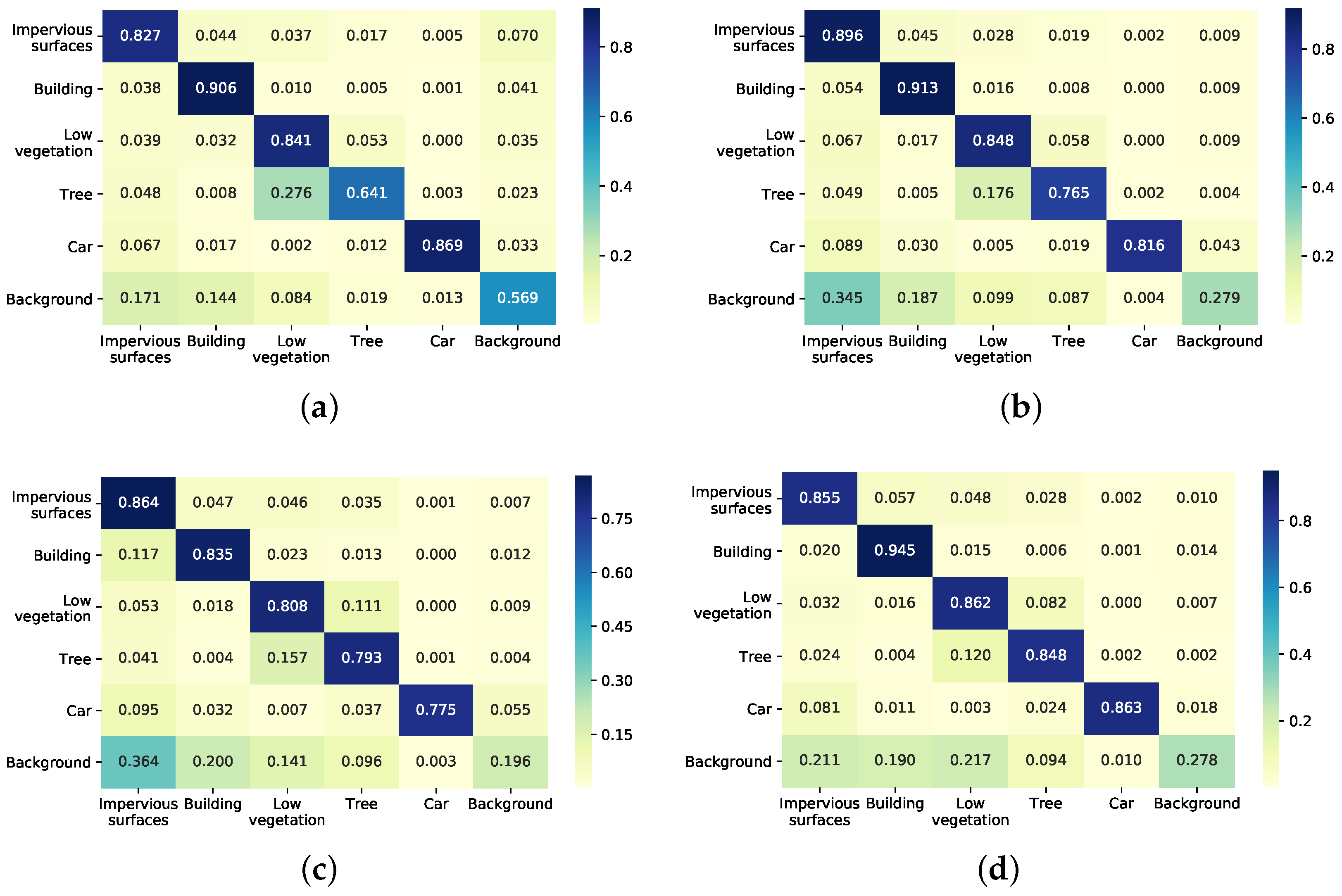
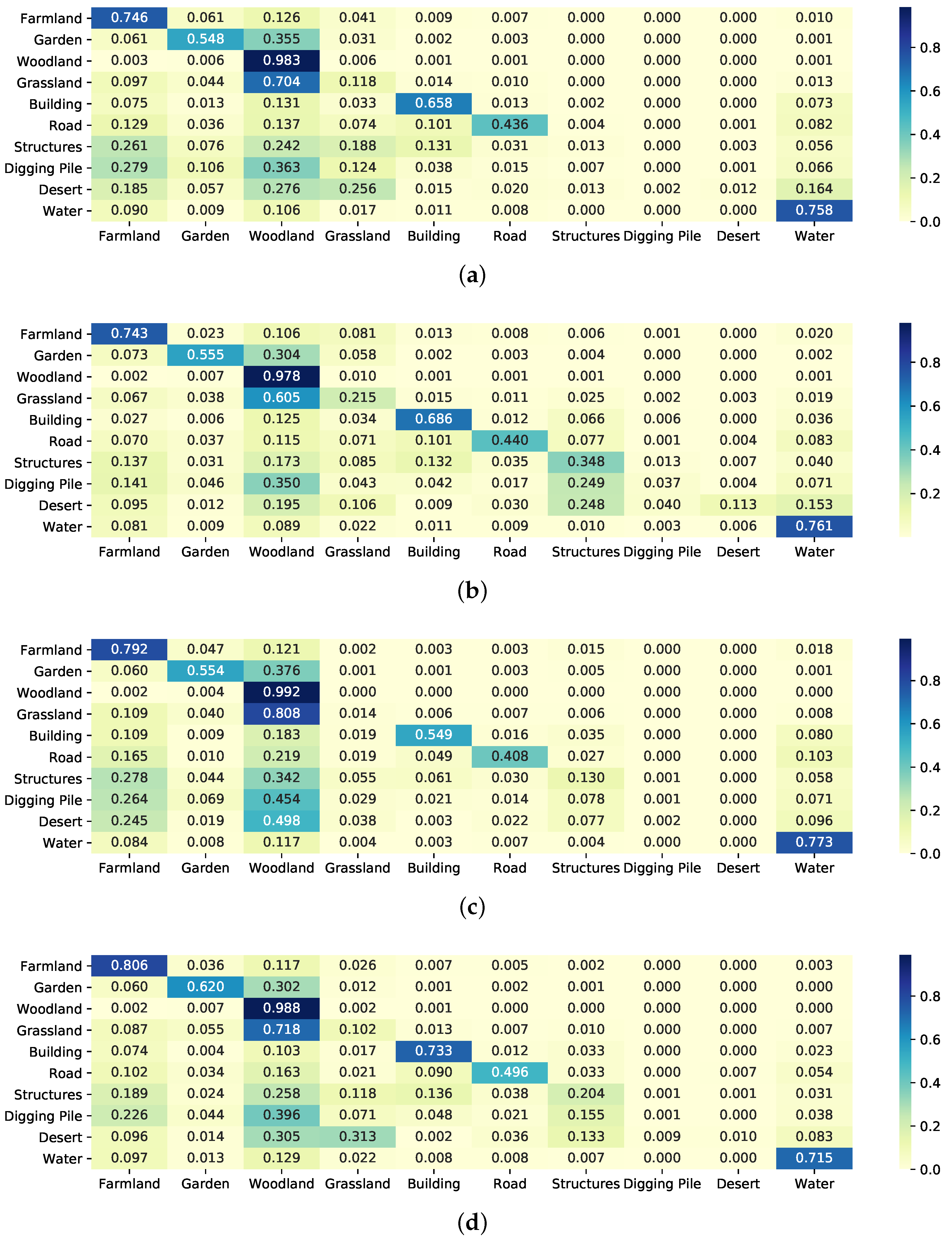
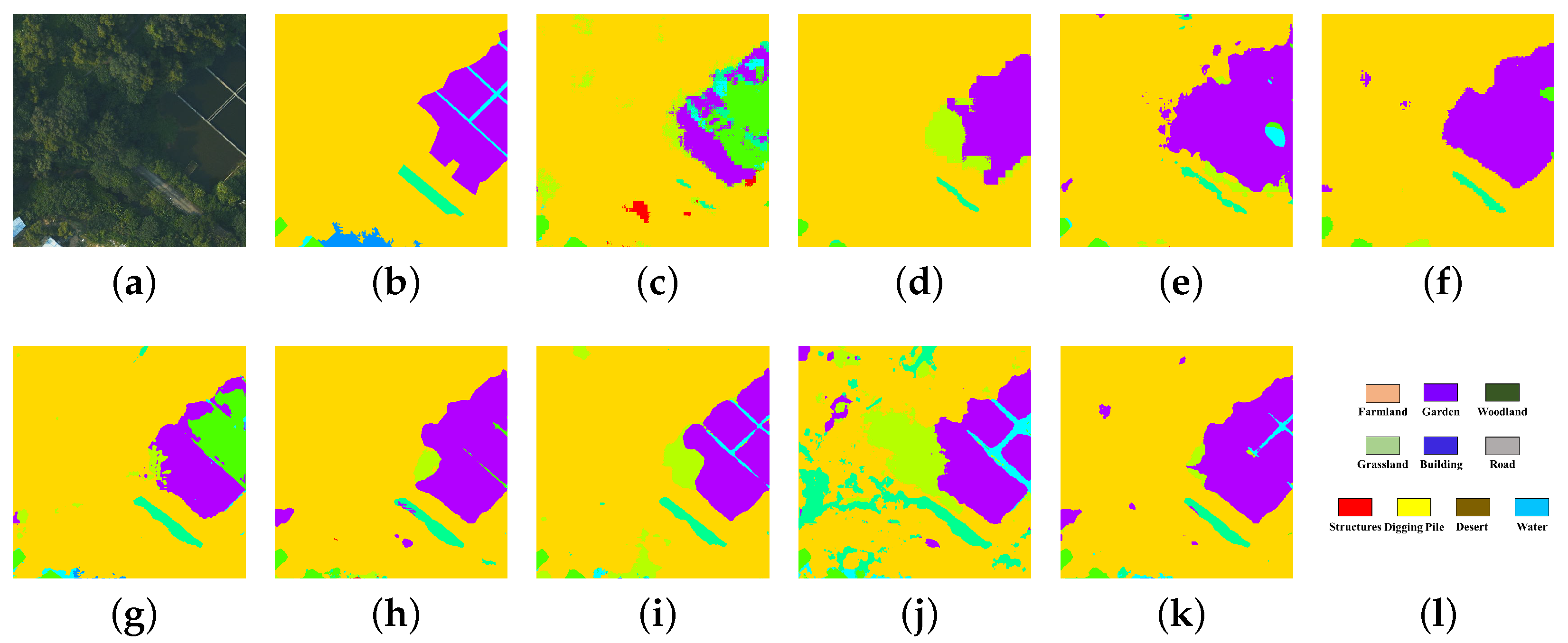
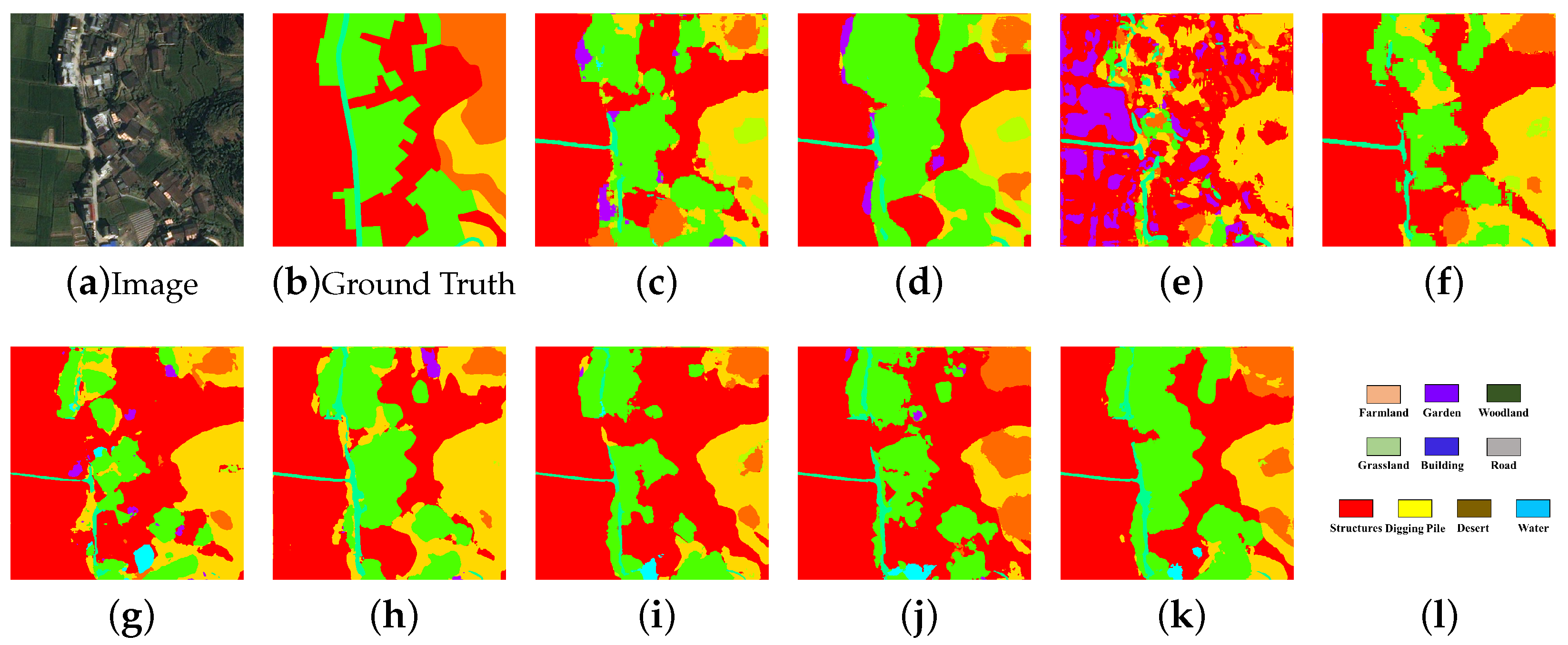
In this section, we explore the effects of different postprocessing fusion methods. We first trained the SDFCNv2 models without using any postprocessing method as the baseline in the three datasets. Then, we evaluate the performance of models that use majority voting or mask-weighted voting for postprocessing, respectively. Besides, we utilize 0°, 90°, 180°, and 270° of rotation (four-direction rotations, denoted as rot90° × 4 in

Table 5. Performances of different post-processing on SDFCNv2 in three experiment datasets. An overlap rate of 0% means there is no post-prediction.

Overlap Rate	rot90° ×4	Weigthed-Mask (Ours)	Potsdam Dataset			EvLab Dataset			Songxi Dataset
			OA	K	mIoU	OA	K	mIoU	OA	K	mIoU
0%	×	×	0.8503	0.8177	0.6782	0.5945	0.5539	0.3208	0.8762	0.7562	0.3980
25%	×	×	0.8573	0.8256	0.6867	0.6016	0.5611	0.3277	0.8784	0.7602	0.4032
	×	✓	0.8576	0.8259	0.6871	0.6025	0.5619	0.3287	0.8787	0.7608	0.4040
	✓	×	0.8639	0.8331	0.6973	0.6137	0.5730	0.3380	0.8815	0.7659	0.4096
	✓	✓	0.8642	0.8334	0.6978	0.6145	0.5738	0.3392	0.8818	0.7665	0.4102

) during the model prediction. Under the circumstance of rotation-based prediction, we further evaluate the effect of the proposed mask-weighted voting postprocessing method. All SDFCNv2 models in this section are trained using spatial-transform-based data augmentation and SSSGT data augmentation methods.

The experimental results of the postprocessing methods in the three datasets are listed in Table 5. Generally, all postprocessing methods (i.e., 25% overlap rate in Table 5) perform better than the baseline (i.e., the 0% overlap rate). Without rotation-based prediction, for the Potsdam, Evlab, and Songxi datasets, the majority voting overlay fusion method outperforms the baseline by 0.85%, 0.69%, and 0.52% in terms of mIoU. Combined with our mask-weighted method, the mIoU values in the three datasets can be further improved by 0.04%, 0.1%, and 0.08%, respectively. After using the rotation-based prediction, it can be seen that the majority voting method can increase the mIoU value by 1.06%, 1.03%, and 0.64%. The performance of the model can be further improved by our mask-weighted method, namely by 0.05%, 0.12%, and 0.06% in the three datasets. In short, whether or not rotation prediction is used, metrics of predicted results utilizing the proposed mask-weighted voting method are slightly superior than not using it. Besides, the prediction with four-direction rotations is an effective way to improve the prediction result. However, it prediction time is four times longer than the prediction without rotations.

5.6. Discussion

By conducting experiments on two public datasets and a real surveying and mapping dataset with different experimental settings, we evaluated the effectiveness of the proposed model structures, gamma-transform-based data augmentation method, and mask-weighted voting postprocessing method, and found that they end up with different progressive results on different datasets. Moreover, the number of parameters in our SDFCNv2 model is much less than the three commonly used models except HRNetV2, as listed in Table 1. With the increasing demand for model efficiency, it becomes very important to develop efficient and effective models with computation-limited resources. Besides, our SDFCNv2 model outperforms other methods under the supervision of a large number of label data. The mIoU value of in the real dataset is lower than 0.45, which is still difficult to be directly used in practical applications.

6. Conclusions

In this work, we introduce an improved semantic segmentation framework called SDFCNv2, including improved model structures, a gamma transform-based data augmentation method, and a mask-weighted voting postprocessing method. In order to evaluate the proposed framework, we conducted several experiments on two public datasets and a real surveying and mapping dataset, namely the Potsdam dataset, the Evlab dataset and the Songxi dataset. Experimental results show that the proposed HBC block and SCFSE module can help to redistribute attention on excavating deep generalized features of the input data. Compared with the previously proposed SDFCNv1 framework, the HBC block can increase the mIoU metric by up to 6.6%, and the SCFSE module can improve the mIoU metric by up to 5.22%. In the second part of the experimental results, we verify that the proposed SSSGT enhancement method helps to generate more diversified distribution of augmented data, prevent overfitting of the model, improve the generalizability of the model, and can further increase the mIoU metric by up to 8.27%. In addition, the improved postprocessing method based on mask-weighted voting decision fusion intentionally avoids low-accuracy prediction in marging region and maintains similar prediction calculation cost, and can further increase the mIoU metric by up to 0.12%.

In the future, we will further reduce model parameters and improve the prediction ability. Moreover, we will also explore transfer learning methods to solve the problem of semantic segmentation when the label samples are insufficient in target domains.

References

1. Cheng, G.; Xie, X.; Han, J.; Guo, L.; Xia, G.S. Remote sensing image scene classification meets deep learning: Challenges, methods, benchmarks, and opportunities. IEEE J. Sel. Top. Appl. Earth Obs. Remote Sens. 2020, 13, 3735–3756. [Google Scholar] [CrossRef]
2. Cheng, G.; Yang, C.; Yao, X.; Guo, L.; Han, J. When deep learning meets metric learning: Remote sensing image scene classification via learning discriminative CNNs. IEEE Trans. Geosci. Remote Sens. 2018, 56, 2811–2821. [Google Scholar] [CrossRef]
3. Helber, P.; Bischke, B.; Dengel, A.; Borth, D. Introducing eurosat: A novel dataset and deep learning benchmark for land use and land cover classification. Int. Geosci. Remote Sens. Symp. 2018, 2018, 204–207. [Google Scholar] [CrossRef]
4. Metzger, M.J.; Bunce, R.G.; Jongman, R.H.; Sayre, R.; Trabucco, A.; Zomer, R. A high-resolution bioclimate map of the world: A unifying framework for global biodiversity research and monitoring. Glob. Ecol. Biogeogr. 2013, 22, 630–638. [Google Scholar] [CrossRef] [Green Version]
5. Taylor, J.R.; Lovell, S.T. Mapping public and private spaces of urban agriculture in Chicago through the analysis of high-resolution aerial images in Google Earth. Landsc. Urban Plan. 2012, 108, 57–70. [Google Scholar] [CrossRef]
6. Benediktsson, J.; Chanussot, J.; Moon, W.M. Advances in Very-High-Resolution Remote Sensing. Proc. IEEE 2013, 101, 566–569. [Google Scholar] [CrossRef]
7. Zhang, X.; Wang, T.; Chen, G.; Tan, X.; Zhu, K. Convective Clouds Extraction From Himawari-8 Satellite Images Based on Double-Stream Fully Convolutional Networks. IEEE Geosci. Remote Sens. Lett. 2019, 17, 553–557. [Google Scholar] [CrossRef]
8. Lateef, F.; Ruichek, Y. Survey on semantic segmentation using deep learning techniques. Neurocomputing 2019, 338, 321–348. [Google Scholar] [CrossRef]
9. Long, J.; Shelhamer, E.; Darrell, T. Fully Convolutional Networks for Semantic Segmentation. IEEE Trans. Pattern Anal. Mach. Intell. 2015, 39, 640–651. [Google Scholar] [CrossRef]
10. Ronneberger, O.; Fischer, P.; Brox, T. U-Net: Convolutional Networks for Biomedical Image Segmentation; Miccai; Springer: Berlin, Germany, 2015; pp. 234–241. [Google Scholar] [CrossRef] [Green Version]
11. Badrinarayanan, V.; Kendall, A.; Cipolla, R. SegNet: A Deep Convolutional Encoder-Decoder Architecture for Image Segmentation. IEEE Trans. Pattern Anal. Mach. Intell. 2017, 39, 2481–2495. [Google Scholar] [CrossRef]
12. Zhao, H.; Shi, J.; Qi, X.; Wang, X.; Jia, J. Pyramid scene parsing network. In Proceedings of the IEEE Conference on Computer Vision and Pattern Recognition, Honolulu, HI, USA, 21–26 July 2017; pp. 2881–2890. [Google Scholar]
13. Lin, G.; Milan, A.; Shen, C.; Reid, I. RefineNet: Multi-path refinement networks for high-resolution semantic segmentation. In Proceedings of the 30th IEEE Conference on Computer Vision and Pattern Recognition, Honolulu, HI, USA, 21–26 July 2017; pp. 5168–5177. [Google Scholar] [CrossRef] [Green Version]
14. Chen, L.C.; Papandreou, G.; Kokkinos, I.; Murphy, K.; Yuille, A.L. DeepLab: Semantic Image Segmentation with Deep Convolutional Nets, Atrous Convolution, and Fully Connected CRFs. IEEE Trans. Pattern Anal. Mach. Intell. 2018, 40, 834–848. [Google Scholar] [CrossRef]
15. Sun, K.; Zhao, Y.; Jiang, B.; Cheng, T.; Xiao, B.; Liu, D.; Mu, Y.; Wang, X.; Liu, W.; Wang, J. High-resolution representations for labeling pixels and regions. arXiv 2019, arXiv:1904.04514. [Google Scholar]
16. Ma, L.; Liu, Y.; Zhang, X.; Ye, Y.; Yin, G.; Johnson, B.A. Deep learning in remote sensing applications: A meta-analysis and review. ISPRS J. Photogramm. Remote Sens. 2019, 152, 166–177. [Google Scholar] [CrossRef]
17. Yuan, Q.; Shen, H.; Li, T.; Li, Z.; Li, S.; Jiang, Y.; Xu, H.; Tan, W.; Yang, Q.; Wang, J.; et al. Deep learning in environmental remote sensing: Achievements and challenges. Remote Sens. Environ. 2020, 241, 111716. [Google Scholar] [CrossRef]
18. Talukdar, S.; Singha, P.; Mahato, S.; Shahfahad; Pal, S.; Liou, Y.A.; Rahman, A. Land-use land-cover classification by machine learning classifiers for satellite observations—A review. Remote Sens. 2020, 12, 1135. [Google Scholar] [CrossRef] [Green Version]
19. Vali, A.; Comai, S.; Matteucci, M. Deep learning for land use and land cover classification based on hyperspectral and multispectral earth observation data: A review. Remote Sens. 2020, 12, 2495. [Google Scholar] [CrossRef]
20. Hoeser, T.; Bachofer, F.; Kuenzer, C. Object detection and image segmentation with deep learning on earth observation data: A review-part II: Applications. Remote Sens. 2020, 12, 1667. [Google Scholar] [CrossRef]
21. Saha, S.; Mou, L.; Qiu, C.; Zhu, X.X.; Bovolo, F.; Bruzzone, L. Unsupervised Deep Joint Segmentation of Multitemporal High-Resolution Images. IEEE Trans. Geosci. Remote Sens. 2020, 58, 8780–8792. [Google Scholar] [CrossRef]
22. Mou, L.; Hua, Y.; Zhu, X.X. Relation Matters: Relational Context-Aware Fully Convolutional Network for Semantic Segmentation of High-Resolution Aerial Images. IEEE Trans. Geosci. Remote Sens. 2020, 58, 7557–7569. [Google Scholar] [CrossRef]
23. Hua, Y.; Marcos, D.; Mou, L.; Zhu, X.X.; Tuia, D. Semantic Segmentation of Remote Sensing Images With Sparse Annotations. IEEE Geosci. Remote Sens. Lett. 2021. [Google Scholar] [CrossRef]
24. Zhong, Y.; Fei, F.; Liu, Y.; Zhao, B.; Jiao, H.; Zhang, L. SatCNN: Satellite image dataset classification using agile convolutional neural networks. Remote Sens. Lett. 2017, 8, 136–145. [Google Scholar] [CrossRef]
25. Ni, W.; Gao, X.; Wang, Y. Single satellite image dehazing via linear intensity transformation and local property analysis. Neurocomputing 2016, 175, 25–39. [Google Scholar] [CrossRef]
26. Yu, H.; Yang, W.; Xia, G.S.; Liu, G. A Color-Texture-Structure Descriptor for High-Resolution Satellite Image Classification. Remote Sens. 2016, 8, 259. [Google Scholar] [CrossRef] [Green Version]
27. Mohammadimanesh, F.; Salehi, B.; Mahdianpari, M.; Gill, E.; Molinier, M. A new fully convolutional neural network for semantic segmentation of polarimetric SAR imagery in complex land cover ecosystem. ISPRS J. Photogramm. Remote Sens. 2019, 151, 223–236. [Google Scholar] [CrossRef]
28. Diakogiannis, F.I.; Waldner, F.; Caccetta, P.; Wu, C. ResUNet-a: A deep learning framework for semantic segmentation of remotely sensed data. ISPRS J. Photogramm. Remote Sens. 2020, 162, 94–114. [Google Scholar] [CrossRef] [Green Version]
29. Flood, N.; Watson, F.; Collett, L. Using a U-net convolutional neural network to map woody vegetation extent from high resolution satellite imagery across Queensland, Australia. Int. J. Appl. Earth Obs. Geoinf. 2019, 82, 101897. [Google Scholar] [CrossRef]
30. Miyoshi, G.T.; Arruda, M.d.S.; Osco, L.P.; Junior, J.M.; Gonçalves, D.N.; Imai, N.N.; Tommaselli, A.M.G.; Honkavaara, E.; Gonçalves, W.N. A novel deep learning method to identify single tree species in UAV-based hyperspectral images. Remote Sens. 2020, 12, 1294. [Google Scholar] [CrossRef] [Green Version]
31. Chen, G.; Zhang, X.; Wang, Q.; Dai, F.; Gong, Y.; Zhu, K. Symmetrical Dense-Shortcut Deep Fully Convolutional Networks for Semantic Segmentation of Very-High-Resolution Remote Sensing Images. IEEE J. Sel. Top. Appl. Earth Obs. Remote Sens. 2018, 11, 1633–1644. [Google Scholar] [CrossRef]
32. Lan, M.; Zhang, Y.; Zhang, L.; Du, B. Global context based automatic road segmentation via dilated convolutional neural network. Inf. Sci. 2020, 535, 156–171. [Google Scholar] [CrossRef]
33. Rottensteiner, F.; Sohn, G.; Jung, J.; Gerke, M.; Baillard, C.; Benitez, S.; Breitkopf, U. The isprs benchmark on urban object classification and 3D building reconstruction. ISPRS Ann. Photogramm. Remote Sens. Spat. Inf. Sci. 2012, 1, 293–298. [Google Scholar] [CrossRef] [Green Version]
34. Chen, L.; Dou, X.; Peng, J.; Li, W.; Sun, B.; Li, H. EFCNet: Ensemble Full Convolutional Network for Semantic Segmentation of High-Resolution Remote Sensing Images. IEEE Geosci. Remote Sens. Lett. 2021. [Google Scholar] [CrossRef]
35. Huang, Z.; Qi, H.; Kang, C.; Su, Y.; Liu, Y. An ensemble learning approach for urban land use mapping based on remote sensing imagery and social sensing data. Remote Sens. 2020, 12, 3254. [Google Scholar] [CrossRef]
36. Li, J.; Meng, Y.; Dorjee, D.; Wei, X.; Zhang, Z.; Zhang, W. Automatic Road Extraction from Remote Sensing Imagery Using Ensemble Learning and Postprocessing. IEEE J. Sel. Top. Appl. Earth Obs. Remote Sens. 2021, 14, 10535–10547. [Google Scholar] [CrossRef]
37. Luo, W.; Li, Y.; Urtasun, R.; Zemel, R. Understanding the effective receptive field in deep convolutional neural networks. In Proceedings of the 30th International Conference on Neural Information Processing Systems, Barcelona, Spain, 5–10 December 2019; pp. 4967–4970. [Google Scholar]
38. Szegedy, C.; Vanhoucke, V.; Ioffe, S.; Shlens, J.; Wojna, Z. Rethinking the Inception Architecture for Computer Vision. In Proceedings of the IEEE Conference on Computer Vision and Pattern Recognition, Las Vegas, NV, USA, 26 June–1 July 2016; pp. 2818–2826. [Google Scholar] [CrossRef] [Green Version]
39. He, K.; Zhang, X.; Ren, S.; Sun, J. Deep Residual Learning for Image Recognition. In Proceedings of the 2016 IEEE Conference on Computer Vision and Pattern Recognition (CVPR), Las Vegas, NV, USA, 26 June–1 July 2016. [Google Scholar] [CrossRef] [Green Version]
40. Tolias, G.; Sicre, R.; Jégou, H. Particular object retrieval with integral max-pooling of CNN activations. arXiv 2015, arXiv:1511.05879. [Google Scholar]
41. Chen, L.C.; Zhu, Y.; Papandreou, G.; Schroff, F.; Adam, H. Encoder-decoder with atrous separable convolution for semantic image segmentation. Lect. Notes Comput. Sci. 2018, 11211, 833–851. [Google Scholar] [CrossRef] [Green Version]
42. Chen, L.C.; Papandreou, G.; Schroff, F.; Adam, H. Rethinking Atrous Convolution for Semantic Image Segmentation. arXiv 2017, arXiv:1706.05587. [Google Scholar]
43. Yu, F.; Koltun, V. Multi-scale context aggregation by dilated convolutions. arXiv 2015, arXiv:1511.07122. [Google Scholar]
44. Yu, F.; Koltun, V.; Funkhouser, T. Dilated residual networks. In Proceedings of the IEEE Conference on Computer Vision and Pattern Recognition, Honolulu, HI, USA, 21–26 July 2017; pp. 636–644. [Google Scholar] [CrossRef] [Green Version]
45. Liu, S.; Huang, D.; Wang, Y. Receptive Field Block Net for Accurate and Fast Object Detection. Lect. Notes Comput. Sci. 2018, 11215, 404–419. [Google Scholar] [CrossRef] [Green Version]
46. Mehta, S.; Rastegari, M.; Shapiro, L.; Hajishirzi, H. ESPNetv2: A light-weight, power efficient, and general purpose convolutional neural network. In Proceedings of the IEEE/CVF Conference on Computer Vision and Pattern Recognition, Long Beach, CA, USA, 16–20 June 2019; pp. 9182–9192. [Google Scholar] [CrossRef] [Green Version]
47. Takikawa, T.; Acuna, D.; Jampani, V.; Fidler, S. Gated-scnn: Gated shape cnns for semantic segmentation. In Proceedings of the IEEE/CVF International Conference on Computer Vision, Seoul, Korea, 27 October–2 November 2019; pp. 5229–5238. [Google Scholar]
48. Li, Y.; Chen, Y.; Wang, N.; Zhang, Z.X. Scale-aware trident networks for object detection. In Proceedings of the IEEE/CVF International Conference on Computer Vision, Seoul, Korea, 27 October–2 November 2019; pp. 6053–6062. [Google Scholar] [CrossRef] [Green Version]
49. Liu, W.; Lee, J. A 3-D Atrous Convolution Neural Network for Hyperspectral Image Denoising. IEEE Trans. Geosci. Remote Sens. 2019, 57, 5701–5715. [Google Scholar] [CrossRef]
50. Chen, H.; Lin, M.; Zhang, H.; Yang, G.; Xia, G.S.; Zheng, X.; Zhang, L. Multi-level fusion of the multi-receptive fields contextual networks and disparity network for pairwise semantic stereo. In Proceedings of the 2019 IEEE International Geoscience and Remote Sensing Symposium, Yokohama, Japan, 28 July–2 August 2019; pp. 4967–4970. [Google Scholar]
51. Chen, X.; Li, Z.; Jiang, J.; Han, Z.; Deng, S.; Li, Z.; Fang, T.; Huo, H.; Li, Q.; Liu, M. Adaptive Effective Receptive Field Convolution for Semantic Segmentation of VHR Remote Sensing Images. IEEE Trans. Geosci. Remote Sens. 2021, 59, 3532–3546. [Google Scholar] [CrossRef]
52. Vaswani, A.; Shazeer, N.; Parmar, N.; Uszkoreit, J.; Jones, L.; Gomez, A.N.; Kaiser, Ł.; Polosukhin, I. Attention is all you need. Adv. Neural Inf. Process. Syst. 2017, 2017, 5999–6009. [Google Scholar]
53. Hu, J.; Shen, L.; Sun, G. Squeeze-and-Excitation Networks. In Proceedings of the IEEE Computer Society Conference on Computer Vision and Pattern Recognition, Salt Lake City, UT, USA, 18–22 June 2018; pp. 7132–7141. [Google Scholar] [CrossRef] [Green Version]
54. Roy, A.G.; Navab, N.; Wachinger, C. Recalibrating fully convolutional networks with spatial and channel “squeeze and excitation” blocks. IEEE Trans. Med. Imaging 2018, 38, 540–549. [Google Scholar] [CrossRef] [PubMed]
55. Woo, S.; Park, J.; Lee, J.Y.; Kweon, I.S. CBAM: Convolutional block attention module. Lect. Notes Comput. Sci. 2018, 11211, 3–19. [Google Scholar] [CrossRef] [Green Version]
56. Fu, J.; Liu, J.; Tian, H.; Li, Y.; Bao, Y.; Fang, Z.; Lu, H. Dual attention network for scene segmentation. In Proceedings of the IEEE/CVF Conference on Computer Vision and Pattern Recognition, Long Beach, CA, USA, 16–20 June 2019; pp. 3141–3149. [Google Scholar] [CrossRef] [Green Version]
57. He, K.; Zhang, X.; Ren, S.; Sun, J. Identity Mappings in Deep Residual Networks. In European Conference on Computer Vision; Leibe, B., Matas, J., Sebe, N., Welling, M., Eds.; Springer International Publishing: Cham, Switzerland, 2016; pp. 630–645. [Google Scholar]
58. Zhang, M.; Hu, X.; Zhao, L.; Lv, Y.; Luo, M.; Pang, S. Learning dual multi-scale manifold ranking for semantic segmentation of high-resolution images. Remote Sens. 2017, 9, 500. [Google Scholar] [CrossRef] [Green Version]
59. Kingma, D.P.; Ba, J.L. Adam: A method for stochastic optimization. In Proceedings of the 3rd International Conference on Learning Representations, ICLR 2015—Conference Track Proceedings, San Diego, CA, USA, 7–9 May 2015. [Google Scholar]
60. Thompson, W.D.; Walter, S.D. A rEAPPRAISAL of the kappa coefficient. J. Clin. Epidemiol. 1988, 41, 949–958. [Google Scholar] [CrossRef]
61. Berman, M.; Rannen Triki, A.; Blaschko, M.B. The lovász-softmax loss: A tractable surrogate for the optimization of the intersection-over-union measure in neural networks. In Proceedings of the IEEE Conference on Computer Vision and Pattern Recognition, Salt Lake City, UT, USA, 18–22 June 2018; pp. 4413–4421. [Google Scholar]
Figure 1. Convolutional layer with different dilated rates. Region covered in dark blue indicates the receptive field. When r = 1, the RF size of a 3 × 3 convolutional filter is equal to 3. When r = 2, the RF size increase to 5. When r = 3, the RF size is equal to 7.
Remotesensing 13 04902 g001
Figure 2. SE block and scSE block. (a) SE block; (b) scSE block.
Remotesensing 13 04902 g002
Figure 3. The backbone structure of SDFCN v2 model. The black arrow in the figure indicates a shortcut connection.
Remotesensing 13 04902 g003
Figure 4. Structures of the Hybrid Basic Convolutional (HBC) Block and the Identity Mapping Hybrid Basic Convolutional (IMHBC) Block. (a) Hybrid Basic Convolutional (HBC) Block; (b) Identity Mapping Hybrid Basic Convolutional (IMHBC) Block.
Remotesensing 13 04902 g004
Figure 5. Spatial and Channel Fusion Squeeze-and-Excitation (SCFSE) Module. The Channel-wise branch is used to recalibrate feature map in a channel-wise manner. The Spatial-wise branches are used to recalibrate features on the X-axis and Y-axis, respectively.
Remotesensing 13 04902 g005
Figure 6. Results of different data augmentation methods based on global gamma transform (GGT), spectral-independent gamma transform (SIGT), and our spectral-specific stochastic gamma transform (SSSGT).
Remotesensing 13 04902 g006
Figure 7. Average accuracy distribution of feature maps at 512 × 512 patch-size on different datasets. (ac) are accuracy distributions on testsets of the Potsdam, the Evlab, and the Songxi dataset.
Remotesensing 13 04902 g007
Figure 8. An illustration of decision fusion post-processing via mask-weighted voting.
Remotesensing 13 04902 g008
Figure 9. DOMs and the corresponding full-covered label vector data in Songxi County. (a) shows DOMs in Songxi dataset; (b) shows vector data of the Songxi dataset; (c) is the legend of the Songxi dataset.
Remotesensing 13 04902 g009
Figure 10. Our proposed SDFCNv2 framework. It includes constructing training datasets from original RS images with labelled vector data, model training and model inference process.
Remotesensing 13 04902 g010
Figure 11. Example image, corresponding label and legend of two public datasets, the ISPRS Potsdam dataset and Evlab dataset. (a) the Potsdam dataset; (b) one image in Potsdam dataset; (c) corresponding ground truth; (d) legend of Potsdam dataset; (e) one image in Evlab dataset; (f) corresponding ground truth; (g) legend of Evlab dataset.
Remotesensing 13 04902 g011
Figure 12. Receptive fields of the center pixel in SDFCNv1 and SDFCNv2 models. The black rectangular frames denote the theoretical regions of receptive fields. (a) RF of SDFCNv1; (b) RF of SDFCNv1 with image; (c) RF of SDFCNv2; (d) RF of SDFCNv2 with image.
Remotesensing 13 04902 g012
Figure 13. Confusion matrices on the Potsdam dataset. (a) PSPNet; (b) HRNet V2; (c) SDFCN V1; (d) SDFCNv2+SCFSE.
Remotesensing 13 04902 g013
Figure 14. Confusion matrices on the Evlab dataset. (a) PSPNet; (b) DeepLab V3+; (c) SDFCN V1; (d) SDFCNv2+SCFSE.
Remotesensing 13 04902 g014
Figure 15. Confusion matrices on the Songxi dataset. (a) FCN-8s; (b) PSPNet; (c) SDFCN V1; (d) SDFCNv2+SCFSE.
Remotesensing 13 04902 g015
Figure 16. Segmentation results on the Potsdam dataset with different models. (a) Image; (b) Ground Truth; (c) FCN-8s; (d) PSPNet; (e) Deeplab V3+; (f) HRNet V2; (g) SDFCN V1; (h) SDFCNv2; (i) SDFCNv2+SE; (j) SDFCNv2+scSE; (k) SDFCNv2+SCFSE; (l) Legend.
Remotesensing 13 04902 g016
Figure 17. Segmentation results on the Evlab dataset with different models. (a) Image; (b) Ground Truth; (c) FCN-8s; (d) PSPNet; (e) Deeplab V3+; (f) HRNet V2; (g) SDFCN V1; (h) SDFCNv2; (i) SDFCNv2+SE; (j) SDFCNv2+scSE; (k) SDFCNv2+SCFSE; (l) Legend.
Remotesensing 13 04902 g017
Figure 18. Segmentation results on Songxi dataset with different models. (a) Image; (b) Ground Truth; (c) FCN-8s; (d) PSPNet; (e) Deeplab V3+; (f) HRNet V2; (g) SDFCN V1; (h) SDFCNv2; (i) SDFCNv2+SE; (j) SDFCNv2+scSE; (k) SDFCNv2+SCFSE; (l) Legend.
Remotesensing 13 04902 g018
Figure 19. Training and validation loss curves of SDFCNv2 model using different gamma-transform-based data augmentation methods on different datasets. (a) Training loss curves on Potsdam dataset; (b) Training loss curves on Evlab dataset; (c) Training loss curves on Songxi dataset; (d) Validation loss curves on Potsdam dataset; (e) Validation loss curves on EvLab dataset; (f) Validation loss curves on Songxi dataset.
Remotesensing 13 04902 g019