Article

Improving Estimation of Woody Aboveground Biomass of Sparse Mixed Forest over Dryland Ecosystem by Combining Landsat-8, GaoFen-2, and UAV Imagery

1
School of Surveying and Land Information Engineering, Henan Polytechnic University, Jiaozuo 454003, China
2
Key Laboratory of Soil and Water Conservation on the Loess Plateau of Ministry of Water Resources, Yellow River Institute of Hydraulic Research, Zhengzhou 450003, China
3
Key Laboratory of Digital Earth Science, Aerospace Information Research Institute, China Academy of Sciences, Beijing 100190, China
*
Author to whom correspondence should be addressed.
Remote Sens. 2021, 13(23), 4859; https://doi.org/10.3390/rs13234859
Submission received: 27 September 2021 / Revised: 22 November 2021 / Accepted: 23 November 2021 / Published: 30 November 2021

Abstract

:
Sparse mixed forest with trees, shrubs, and green herbaceous vegetation is a typical landscape in the afforestation areas in northwestern China. It is a great challenge to accurately estimate the woody aboveground biomass (AGB) of a sparse mixed forest with heterogeneous woody vegetation types and background types. In this study, a novel woody AGB estimation methodology (VI-AGB model stratified based on herbaceous vegetation coverage) using a combination of Landsat-8, GaoFen-2, and unmanned aerial vehicle (UAV) images was developed. The results show the following: (1) the woody and herbaceous canopy can be accurately identified using the object-based support vector machine (SVM) classification method based on UAV red-green-blue (RGB) images, with an average overall accuracy and kappa coefficient of 93.44% and 0.91, respectively; (2) compared with the estimation uncertainties of the woody coverage-AGB models without considering the woody vegetation types (RMSE = 14.98 t∙ha−1 and rRMSE = 96.31%), the woody coverage-AGB models stratified based on five woody species (RMSE = 5.82 t∙ha−1 and rRMSE = 37.46%) were 61.1% lower; (3) of the six VIs used in this study, the near-infrared reflectance of pure vegetation (NIRv)-AGB model performed best (RMSE = 7.91 t∙ha−1 and rRMSE = 50.89%), but its performance was still seriously affected by the heterogeneity of the green herbaceous coverage. The normalized difference moisture index (NDMI)-AGB model was the least sensitive to the background. The stratification-based VI-AGB models considering the herbaceous vegetation coverage derived from GaoFen-2 and UAV images can significantly improve the accuracy of the woody AGB estimated using only Landsat VIs, with the RMSE and rRMSE of 6.6 t∙ha−1 and 42.43% for the stratification-based NIRv-AGB models. High spatial resolution information derived from UAV and satellite images has a great potential for improving the woody AGB estimated using only Landsat images in sparsely vegetated areas. This study presents a practical method of estimating woody AGB in sparse mixed forest in dryland areas.

Graphical Abstract

1. Introduction

Low-carbon emissions have become a major scientific and political issue for the international communities to address global climate change. Carbon sequestration in terrestrial ecosystems can offset parts of anthropogenic CO2 emissions, which has been a strategic plan to achieve indirect emissions reduction and an important way for China to achieve the goal of “carbon neutrality” in the future [1,2]. Arid and semi-arid areas account for more than 40% of the global land area, and the carbon cycle process is highly sensitive to climate change and human activities. Due to there are a large uncertainty in the estimation of vegetation carbon storage in the arid and semi-arid areas, it has become a high interest for numerous scientists to study the advanced method estimating carbon storage of ecosystems in the arid areas [3]. Since 1978, extensive ecological restoration projects such as the Three-North Shelterbelt and Grain for Green have been implemented in arid and semi-arid regions in China; consequently, the area of artificial forests of China is the largest over the world. Therefore, it is very urgent to evaluate the structure and function of the artificial forests in China, especially for the arid and semi-arid areas [4]. Woody aboveground biomass (AGB) is a key indicator for characterizing not only the carbon storage of artificial forests but also ecosystem structure and ecological service functions [5]. Therefore, it is very significant to monitor the woody AGB of artificial forest at a regional scale for assessing the effectiveness of ecological restoration projects implemented in the arid and semi-arid areas in China.
The traditional method of acquiring the woody aboveground biomass (AGB) is mainly based on manual harvesting in field plots. Although the accuracy of the AGB obtained from field measurements is extremely high, it is very time consuming and labor-intensive, and the number of measured sites is also very limited. Thus, it is very difficult to obtain the spatial distribution of the AGB of vegetation in a large area [6]. Because remote sensing has the peculiar characteristic of temporally and spatially continuous observations of the Earth’s surface, it has currently become the main technical method of estimating the woody AGB at the regional scale [5,7]. Based on the types of sensors mounted on the remote sensing platform, the remote sensing data can be divided into optical [8,9], synthetic aperture radar (SAR) [10], and Lidar [11]. Different types of remote sensing data have different physical mechanisms for retrieving the AGB of vegetation, and each has its own advantages and disadvantages [12]. Although the estimation accuracy of the forest AGB is relatively high using LiDAR or SAR, optical remote sensing is still the most widely used method for estimating the forest AGB in a large area due to the high availability and spatial-temporal consistency of its optical satellite imagery at small and medium scales [13]. The ATLAS onboard ICESat-2 was launched in September 2018 [14]. It is used to AGB estimate, and will join BIOMASS [15], NISAR [16], and Tandem-L in the future.
The spectral reflectance or various vegetation indexes have been directly used to develop a forest AGB model in many studies [17,18,19,20,21,22].
However, the spectral signal has a saturation effect for high coverage of woody vegetation, and it can be easily affected by various environmental factors during the radiative processes. Thus, the accuracy of woody AGB estimations obtained using only spectral information is not very satisfactory [23]. To solve this problem, many efforts have been made; for example, the texture [24], rainfall [25], forest age [8], and topography [9] have been gradually combined with the spectral indices to improve the AGB estimation. To reduce the estimation errors caused by the heterogeneity of the woody vegetation types, stratification-based AGB estimation models have been developed for different forest types and tree species [26,27,28], but the classification accuracy affects the woody AGB estimates. The methods used in previous studies have been successfully applied in areas dominated by dense forest. However, most of the plantation forests were located in the arid and semi-arid areas in China, and the coverage of the woody vegetation was relatively low. In this situation, the problem of mixed pixels in satellite observations with a medium resolution (e.g., Landsat at the 30 m scale) inevitably led to an unsatisfactory woody AGB estimation accuracy in sparse artificial forests [6,29]. Consequently, linear spectral mixture analysis (LSMA) was used to retrieve the woody canopy coverage, and then, the woody AGB was estimated based on the relationship between the woody canopy coverage and the AGB [13,30]. However, this method is not suitable for sparse forests with woody and dense green herbaceous vegetation because the coverage of such forests cannot be accurately identified using LSMA because their endmember spectra are very similar.
In order to solve this problem, several researchers began deriving the woody canopy coverage based on high spatial resolution remote sensing imagery [27,31,32,33,34,35,36], and a woody coverage-AGB model was constructed to retrieve the woody AGB. These studies showed that the canopy coverage derived from high-resolution satellite data can effectively improve the estimation accuracy of the woody AGB, and this method has been successfully applied to sparse pure forests [32,37,38]. In northern China, sparse mixed forest containing trees, shrubs, and green herbaceous vegetation is a typical landscape in reforestation areas. It is well known that using remote sensing data to estimate the woody AGB in this specific type of area, i.e., where the woody vegetation types and background types are highly heterogeneous, is a great challenge. Some scholars had provided global scale biomass maps information based on remote sensing for different years [15,39]. Therefore, in this study, a method of accurately estimating the woody AGB of a sparse mixed forest using a combination of satellite imagery with a medium resolution (Landsat-8) and high resolution (GaoFen-2) and unmanned aerial vehicle (UAV) images was developed. The objectives of this study are as follows: (1) to explore the potential of high-resolution images acquired via UAV and GaoFen-2 to obtain accurate woody and herbaceous coverage; (2) to develop a method of accurately estimating the woody AGB of a sparse mixed forest using a combination of field measurements and UAV, GaoFen-2, and Landsat-8 images; (3) to assess the advantages of the newly developed method by comparing the results of the new method with those obtained using only Landsat-8 and using a combination of GaoFen-2 and UAV images.

2. Study Area and Data
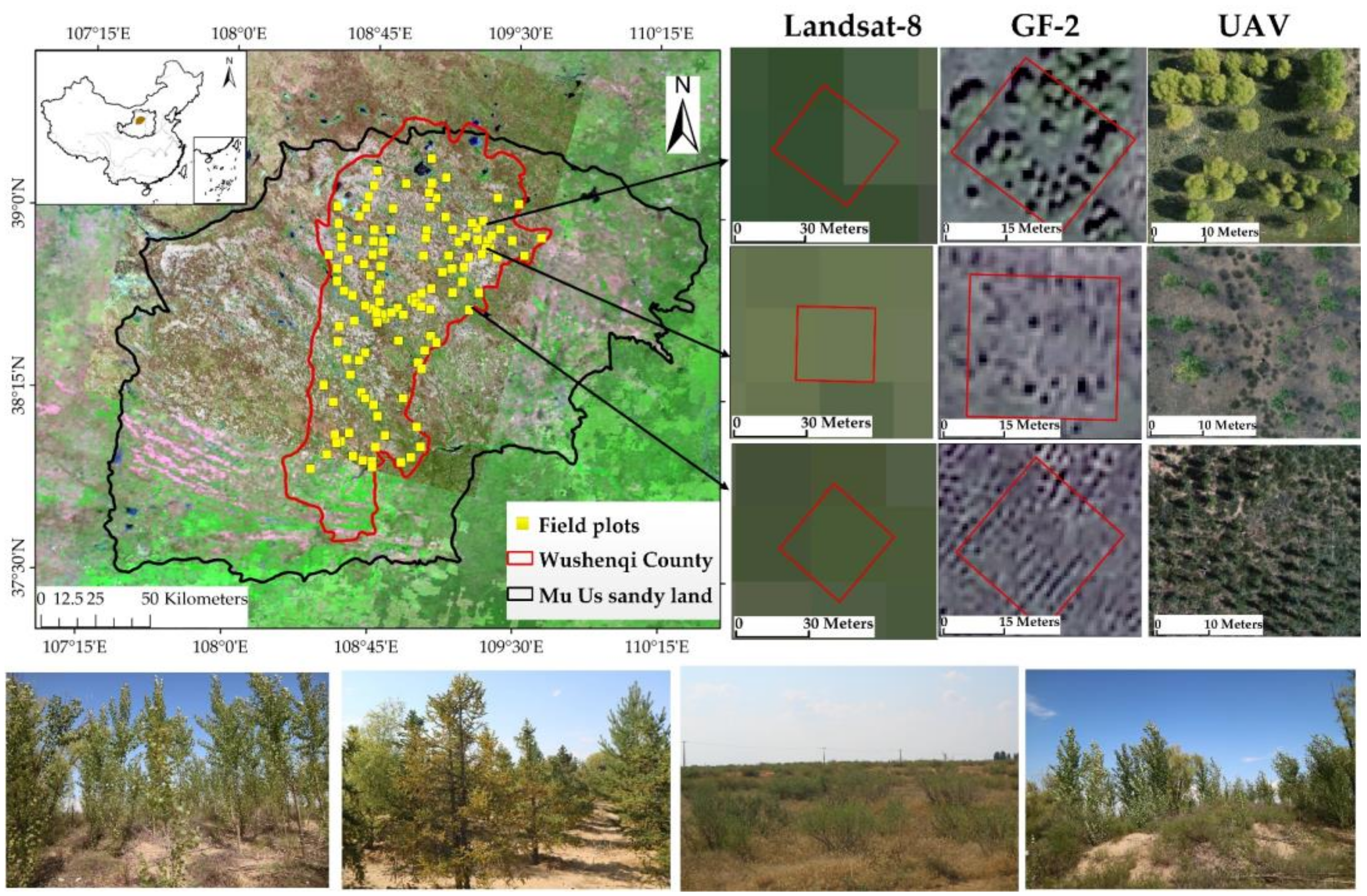
2.1. Study Area

The Mu Us Sandy Land is located in the southeastern part of Ordos City and the northern part on the Loess Plateau (37°27′–39°22′N, 107°20′–111°30′E), covering an area of about 42,200 km2. The multiyear average potential evapotranspiration is 1048.81 mm, the annual average temperature is 6.0–8.5 °C, and the annual average precipitation is 250–400 mm. Due to the historical intensive human activities, the vegetation has been seriously degraded and the living environment has been harsh in this area [40,41]. The coverage of the woody vegetation has increased significantly after nearly 30 years of tree planting and afforestation [42]. The woody species of the artificially planted vegetation in this arid area mainly include Populus alba L., Salix matsudana, Pinus tabuliformis, Artemisia ordosida, and Caragana korshinskii.

2.2. Data and Processing

From 16 to 30 September 2019, a 15-day field survey was carried out in Uxin Qi county located at the Mu Us Sandy Land, and a total of 102 plots were investigated. In each plot, a 30 m × 30 m plot boundary was constructed manually, and the Trimble Real-time Kinematic (RTK) GPS was used to measure four corner coordinates of plot. Species, height, diameter at breast height (DBH), crown diameter (east-west and north-south) for each individual woody vegetation within the plot were recorded and measured. At the same time, the DJI Phantom 4RTK UAV was used to acquire the RGB images (0.1 m) overhead the plot, and the overlap degree of adjacent images was at least 60%. All RGB images were mosaicked using the Photoscan software. It should be noted that GPS signals used to calculate high-accuracy coordinates of UAV RTK and Trimble RTK are from the same continuously operating reference stations (CORS). The spatial distribution of the survey plot is shown in Figure 1.
To guarantee synchronous observation of field and satellite observations, we downloaded Landsat-8 OLI (L1T) surface reflectance data for 21 September 2019, from the Google Earth Engine cloud (GEE) platform, with a spatial resolution of 30 m, and the cloud and cloud shadows in the image were identified based on the F-mask algorithm. The GaoFen-2 satellite image, taken on 20 September 2019, was obtained from the China Center for Resources Satellite Data and Application (http://www.cresda.com/, accessed on 13 November 2021), with a GSD (Ground Sampling Distance) of 0.81 m in panchromatic and 3.24 m in the multispectral bands (PAN: 450–900 nm, B1/blue: 450–520 nm, B2/green: 520–590 nm, B3/red: 630–690 nm, B4/NIR: 770–890 nm).
The UAV, GaoFen-2, and Landsat-8 images were orthorectified based on the same ground control points using the PCI GeoImaging Accelerator (GXL), which is a professional-grade preprocessing software provided by Twenty First Century Aerospace Technology Co., Ltd. This procedure guaranteed the accuracy of the geometric correction for these three remote sensing images with different scales.

3. Methodology

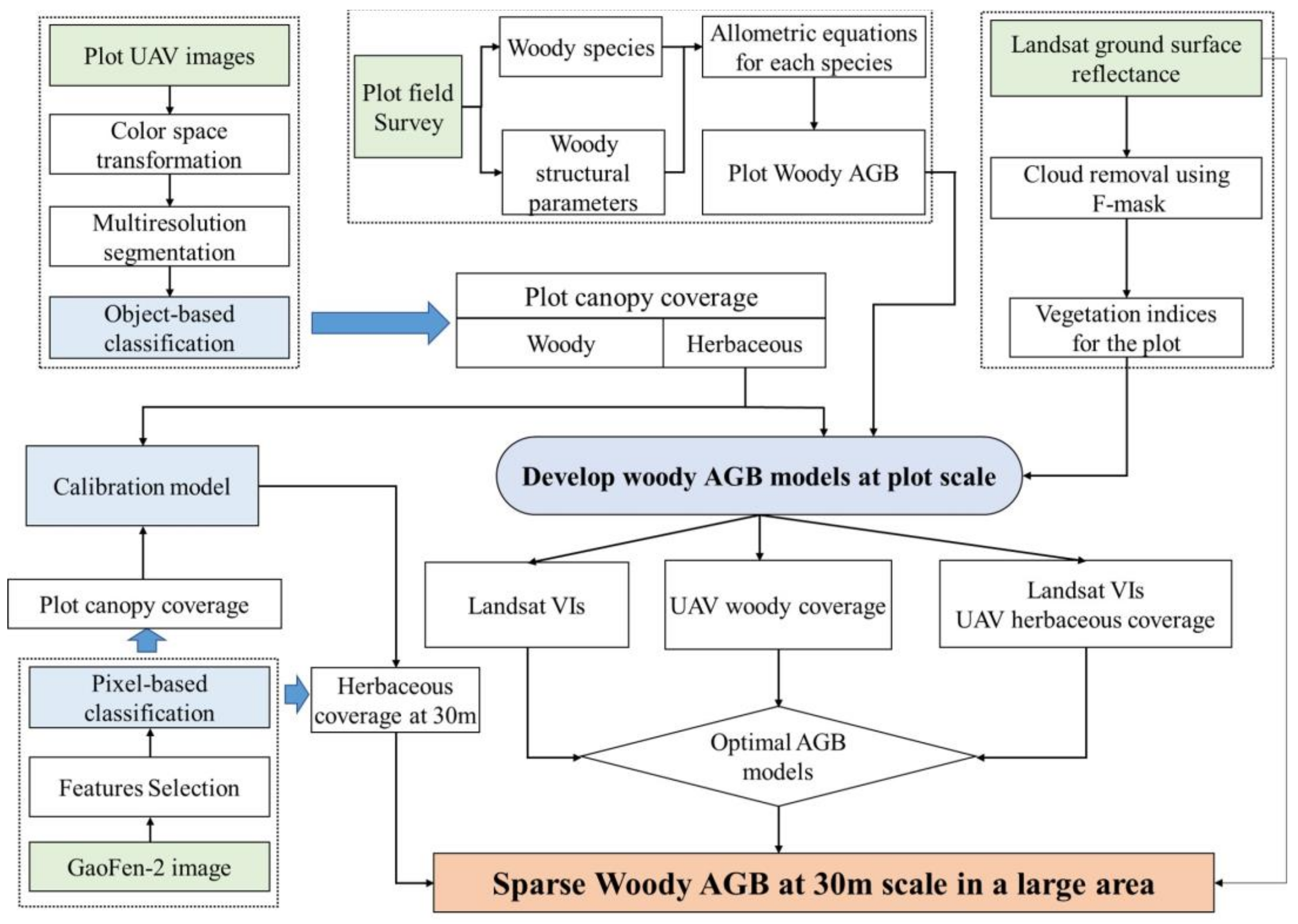
3.1. Overall Methodology

The overall flow scheme of the woody AGB estimation of the sparse mixed forest is shown in Figure 2. It includes the following major steps: (1) calculating the plot-level AGB based on the field measurements and allometric equations for each plot; (2) surveying the woody and herbaceous vegetation coverage based on the classification of the UAV image; (3) developing different plot-level AGB models using the Landsat, UAV, and GaoFen-2 images; (4) calibrating the woody and herbaceous coverage derived from the GaoFen-2 image based on the UAV measurements; (5) validating the accuracies of the AGB estimates derived from the different plot-level AGB models and calibrating the vegetation coverage derived from the GaoFen-2 image. In addition, the sparse woody AGB in a large area was estimated using the optimal AGB model based on the Landsat and GaoFen-2 images.

3.2. Calculation of the Plot-Level Woody AGB Using Woody Structural Parameters

Because the study area is a national key ecological reserve, the harvesting of woody vegetation is not allowed by the local government. Therefore, the allometric equations of the trees and shrubs determined in previous studies based on field measurements in the Mu Us Sandy Land and its adjacent areas [6,8,43] were selected to calculate the plot-level AGB of the woody vegetation. The allometric equations of the five woody species are presented in Table 1. Table 2 shows the descriptive statistics of the AGB data.

3.3. Coverage Survey of the Woody and Herbaceous Vegetation Using UAV RGB Image

For each UAV red-green-blue (RGB) image, 100 samples of all categories including tree, shrub, herbaceous vegetation, bare soil, and shadow were selected by manual visual interpretation, and stratified proportion sampling with a ratio of 6:4 was used to generate training and validation samples for image classification [44].
Hue-Saturation-Value (HSV) color space conversion was performed on the original RGB image. Multiscale segmentation was employed to segment the HSV image, and the spectral and geometric features of the segmented objects were then extracted using eCognition 9.5. We trained the object-based support vector machine (SVM) classification algorithm using the training data, and then we validated the classification results using the validation data.
The coverage of a specific vegetation type is the number of pixels of this vegetation type divided by the total number of pixels in the image. Because there were a lot of shadows covering the herbaceous vegetation and bare soil in the high spatial resolution UAV image, the normalization method was used to correct the coverage of the herbaceous vegetation and bare soil in this study, and the calculation equations used are as follows:
Grass _ new = Grass Grass + Soil × Shadow + Grass
Soil _ new = Soil Grass + Soil × Shadow + Soil
where Grass_new and Soil_new are the corrected coverages of the herbaceous vegetation and bare soil, respectively; Grass, Soil, and Shadow are the original coverages of the herbaceous vegetation, bare soil, and shadows.

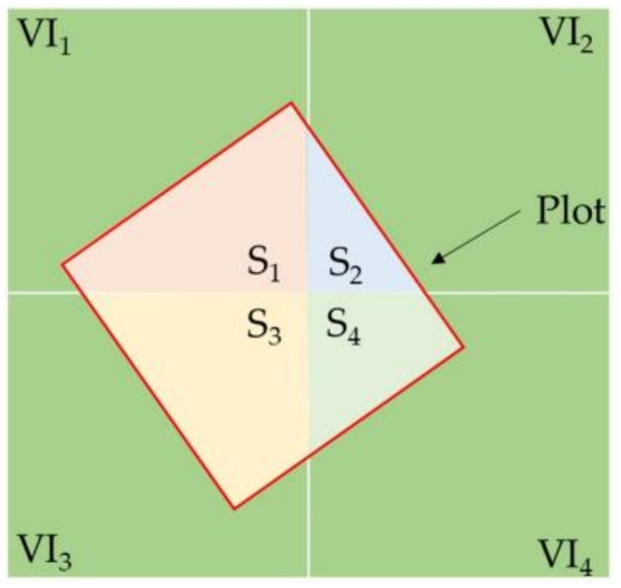
3.4. Development of Different Plot-Level Woody AGB Models Using Landsat-8 and UAV Imagery

Based on previous studies, we selected six commonly used vegetation indices (VIs) that have strong correlations with the vegetation AGB, including the normalized difference vegetation index (NDVI), the ratio vegetation index (RVI), the modified adjusted vegetation index (MSAVI), the tasseled cap transform greenness (TCG), the normalized difference moisture index (NDMI), and the near-infrared reflectance of pure vegetation (NIRv). The tasseled cap transform greenness was calculated according to the equation provided in a previous study [45], and the equations of the other VIs are as follows:
NDVI = NIR R NIR + R
RVI = NIR R
MSAVI = 0.5 × 2 × NIR + 1 2 × NIR + 1 2 8 × NIR RED
NDMI = NIR SWIR 1 NIR + SWIR 1
NIRv = NDVI × NIR
where NIR, R, and SWIR1 are the reflectance in the near infrared (0.845–0.885 μm), red (0.63–0.68 μm), and shortwave infrared (1.56–1.66 μm) bands of the Landsat-8 OLI image, respectively.
As the domain of field plot (30 m × 30 m) did not perfectly match the Landsat pixel at 30 m scale, we used the weighted average method to calculate the plot-level Landsat VI. A schematic diagram of the weighted average method is shown in Figure 3, and the equation used for the calculation is as follows:
V I plot = S i S plot × V I i
where VIplot is the VI corresponding to the field plot, VIi is the VI of the ith pixel covered by the plot range, Splot is the total area of the plot, and Si is the area of the ith pixel within the plot range. The scope of Si was delineated through manual interpretation using Arcmap 10.5.
In this study, in order to explore the potential of using multiscale remote sensing data to estimate the woody AGB of sparse mixed forest, different plot-level woody AGB estimation models were developed using the following three different schemes.
Scheme 1: Woody coverage-AGB model: a linear regression model was built based on the logarithmic transformation of the plot-level woody coverage derived from the UAV classification and logarithmic transformation of the plot-level woody AGB.
Scheme 2: VI-AGB models: linear, logarithmic, exponential, and power regression models were built using the plot-level VIs of the Landsat-8 and plot-level woody AGB.
Scheme 3: Stratification-based VI-AGB models: linear, logarithmic, exponential, and power regression models were built using the plot-level VIs of the Landsat-8 and plot-level woody AGB for the plots with different levels of herbaceous vegetation coverage (0%, 0–30%, >30%) derived from the UAV classification.

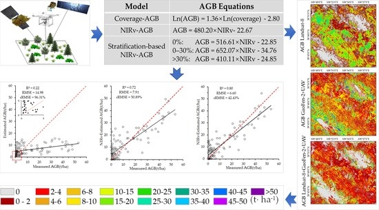
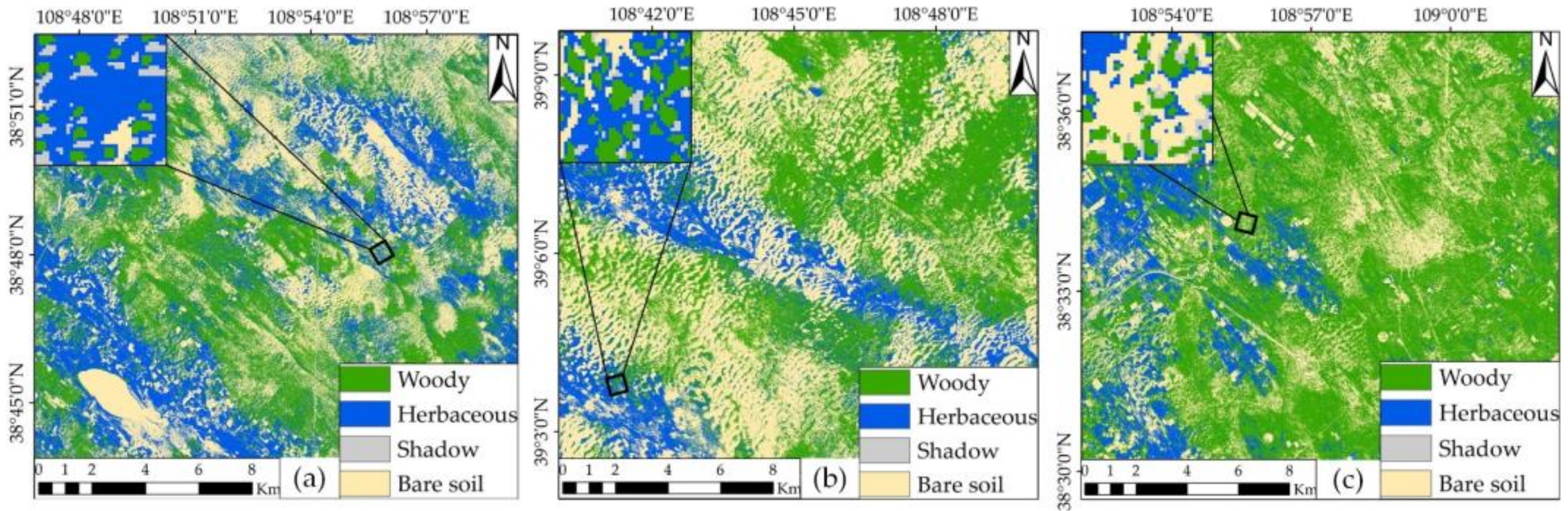
3.5. Regional Simulation of Woody AGB Using Landsat-8 and GaoFen-2 Imagery

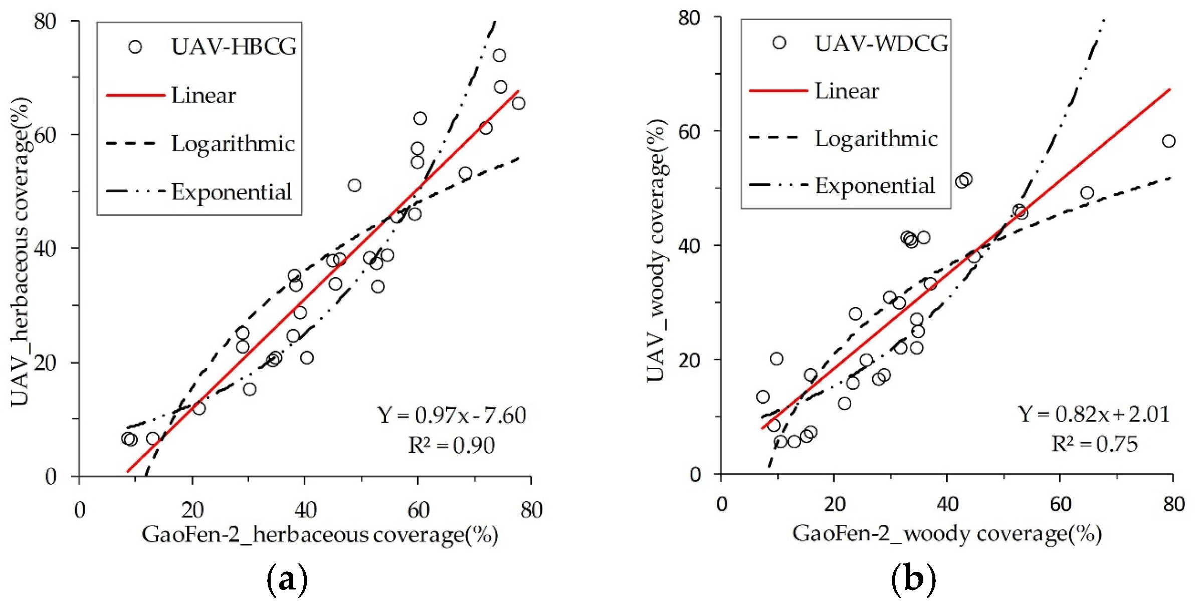
3.5.1. Calibration of Woody and Herbaceous Coverage Derived from the GaoFen-2 Image

The samples of trees and shrubs selected in Section 3.3 were redefined as samples of woody vegetation, and the pixel-based SVM classification method was used to classify the GaoFen-2 image into four surface cover types, including woody, herbaceous, bare soil, and shadow, using ENVI 5.3. The plot-level woody and herbaceous coverage were calculated based on the GaoFen-2 classification. Due to the effect of the shadow cover, the coverages of the herbaceous vegetation and bare soil were also modified using Equations (1) and (2).
In order to reduce the systematic bias of the vegetation coverage derived from the GaoFen-2 image at 0.8 m and the UAV image at 0.05 m, linear, logarithmic, and exponential regression models were built between the woody and herbaceous coverage derived from the GaoFen-2 image and that derived from the UAV image, and the optimal regression model was selected as the calibration model for the woody and herbaceous coverage derived from the GaoFen-2 image. Finally, the woody and herbaceous vegetation coverages at a 30 m scale over the entire study area were generated using the GaoFen-2 classification and calibration model.

3.5.2. Accuracy Assessment of Woody AGB Estimates Using Different Methods

To evaluate the performances of the different woody AGB estimation schemes described in Section 3.4, the plot-level woody AGB estimates derived using the different plot-level models in the three schemes and woody and herbaceous coverages derived from the GaoFen-2 were validated using the plot-level woody AGB measurements. The regional woody AGB estimates at the 30-m scale derived using Landsat-8, GaoFen-2, UAV, and a combination of Landsat-8, GaoFen-2, and UAV were compared, and the potential of using multiscale remote sensing data to estimate the woody AGB of a sparse mixed forest in an arid area was explored and discussed.

4. Results and Analysis

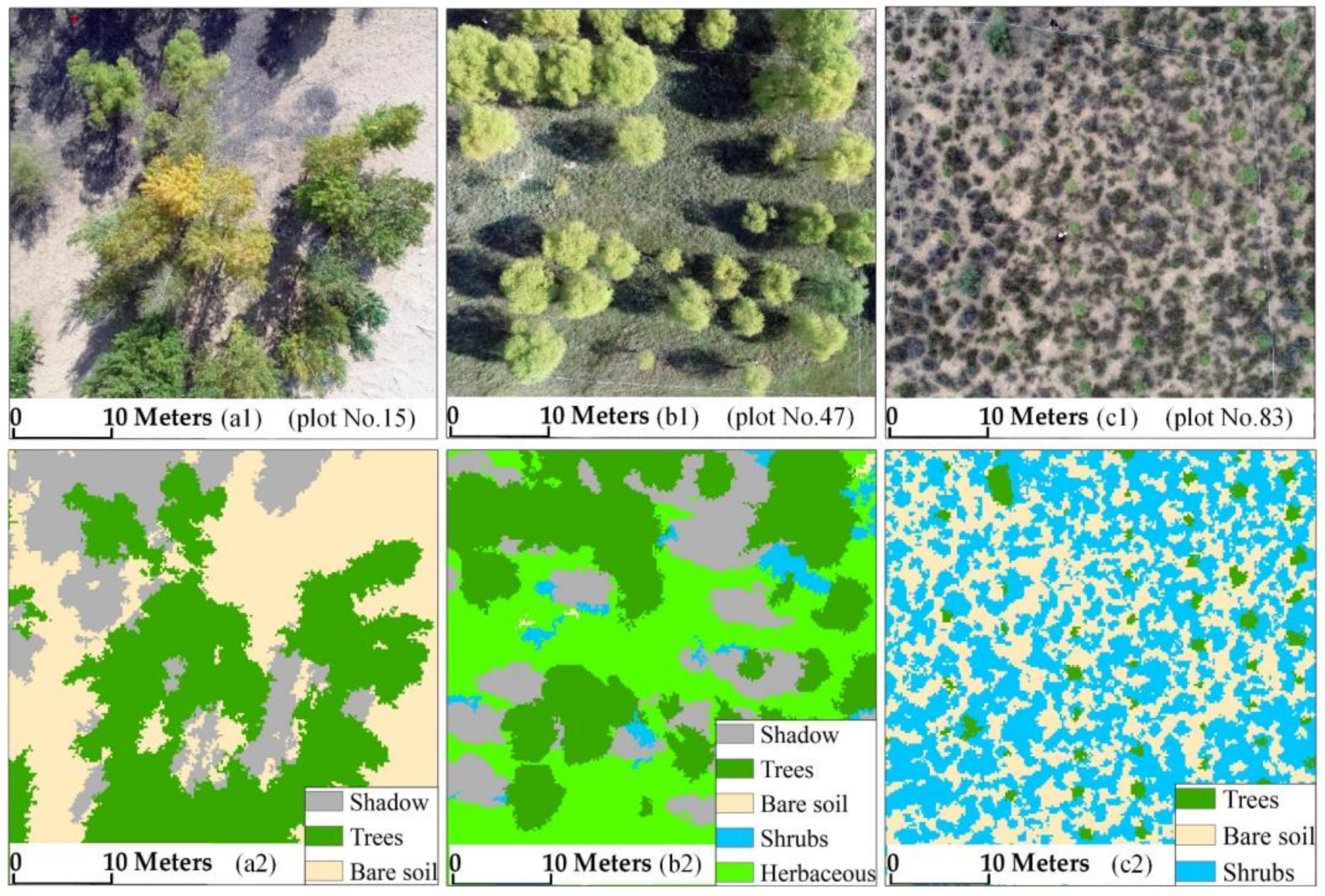
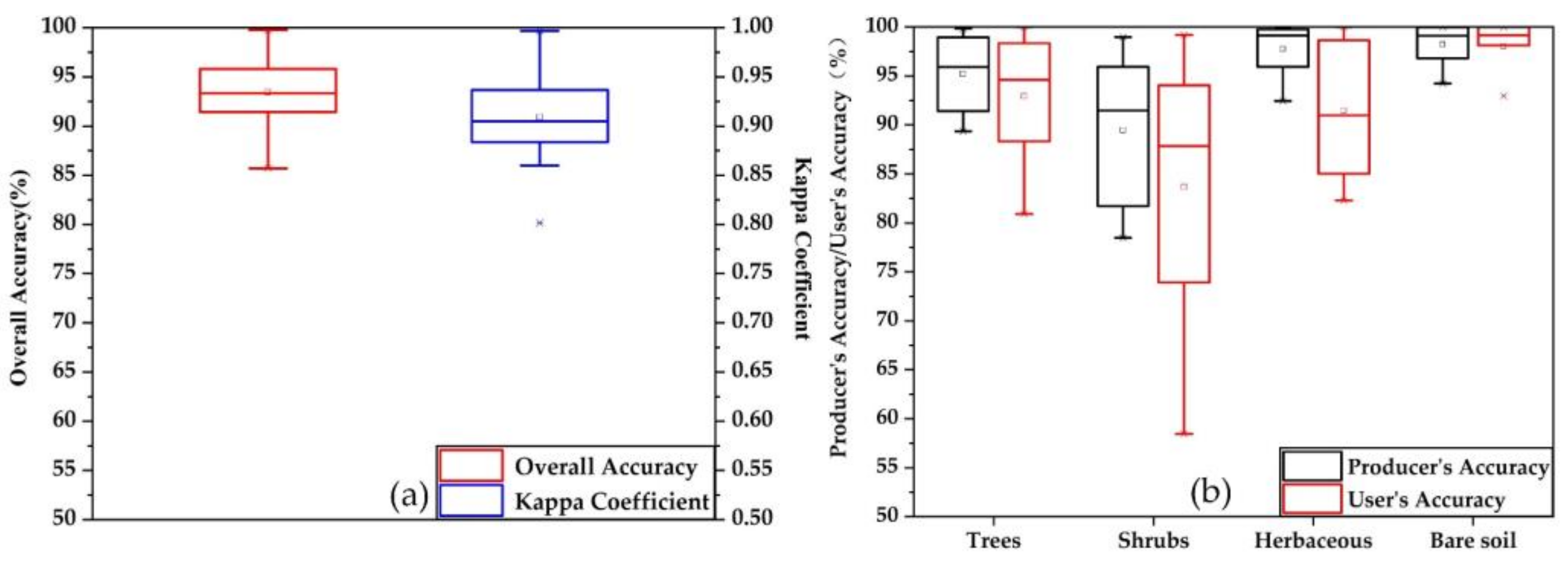
4.1. Classification and Accuracy Assessment of UAV RGB Image

UAV images corresponding to 102 plots were classified in this study (e.g., Figure 4). The classification accuracy of all the UAV images was assessed using the error matrix method [46], and the accuracy metrics of the classification are illustrated in Figure 5. As can be seen, the average overall accuracy and the Kappa coefficient are 93.44% and 0.91, respectively, and the average producer’s accuracy and user’s accuracy are 94.11 and 93.90% for all plots, respectively. It can also be seen that the classification accuracy of the bare soil is the highest, and the classification accuracy of the shrub is the lowest. This classification was then used for calculating the canopy coverage of woody and herbaceous vegetation.

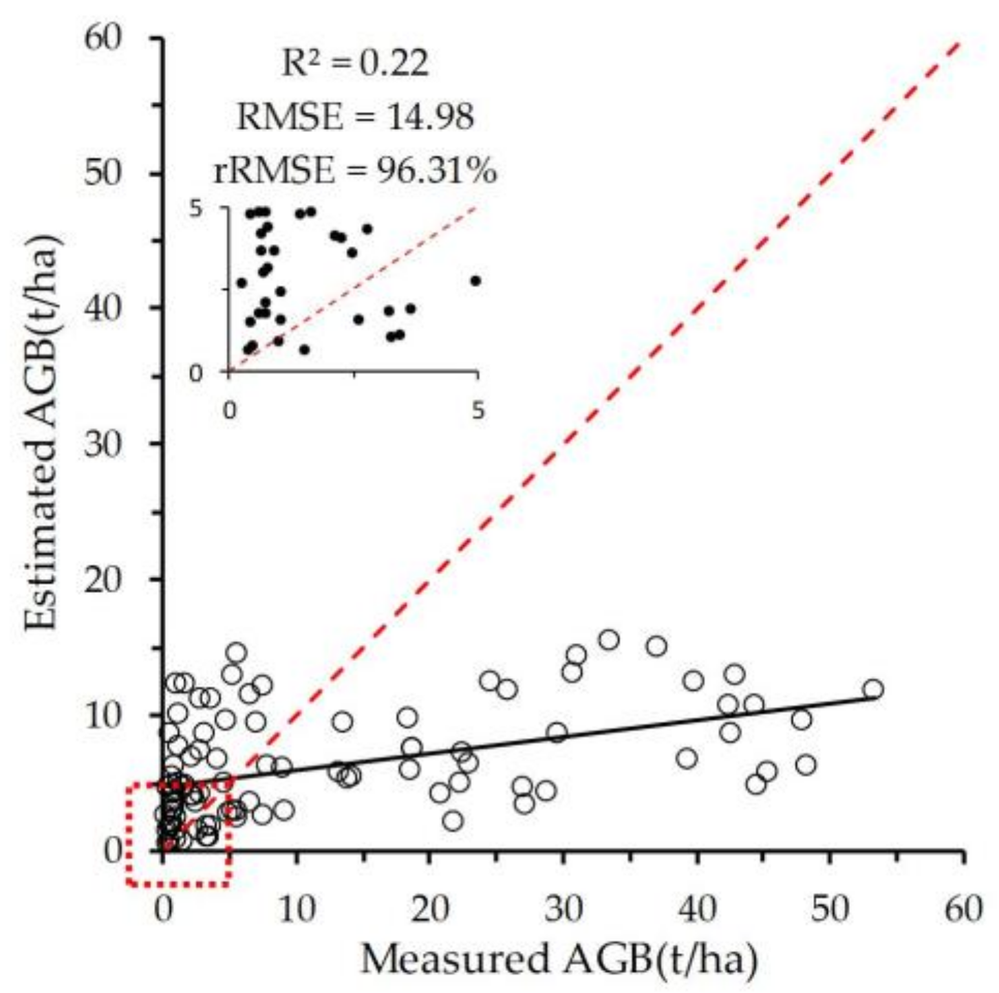
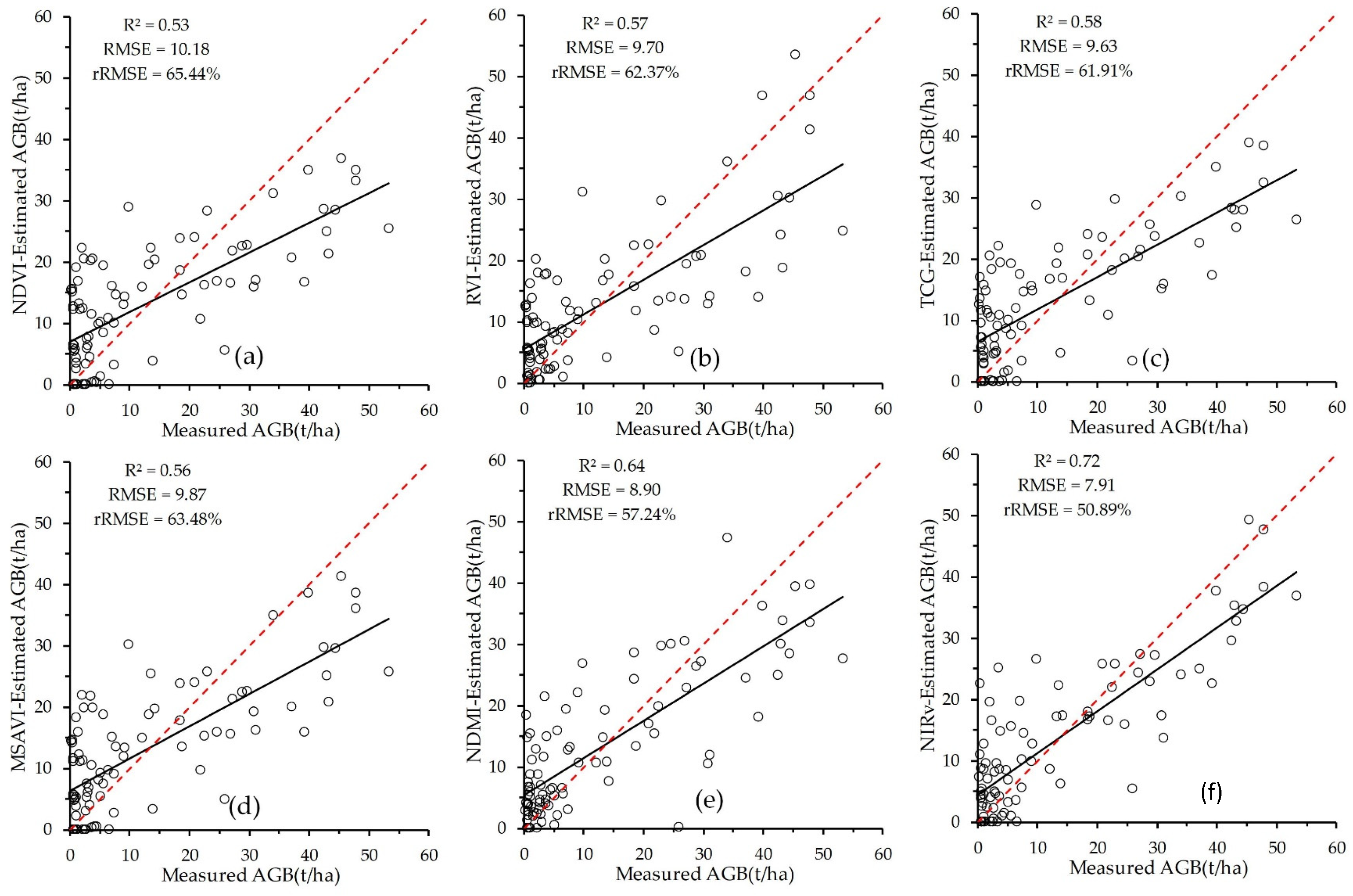
4.2. Plot-Level Woody AGB Models

The canopy coverage of woody vegetation in each plot was used as an independent variable, the AGB was calculated by using AGB allometric equations as a dependent variable, and the canopy coverage woody AGB model was built by combining the logarithms of both sides. Equation (8) is the woody coverage-AGB model for scheme 1, and its determination coefficient R2 is very low.
Ln(AGB) = 1.36 × ln(woody coverage) − 2.80 (R2 = 0.25)
The VI-AGB models using six vegetation indices in scheme 2 are presented in Table 3. It can be seen from Table 3 that the linear regression models based on the vegetation indices are more robust than the regression models that use other functions, and the NIRv has the best performance in terms of explaining the variations in the sparse woody AGB. It should be noted that logarithmic and power regression models cannot be built for the TCG and NDMI as a result of the negative TCG and NDMI values. The stratification-based VI-AGB models in scheme 3 are presented in Table 4. It can be seen that the robustness of the woody AGB model is significantly improved when the heterogeneity of the background of the sparse woody vegetation, namely, the different levels of herbaceous vegetation coverage, are considered.

4.3. Woody and Herbaceous Coverage Derived from GaoFen-2 Image

The pixel-based SVM classification of the GaoFen-2 image in three subregions is shown in Figure 6, and the woody and herbaceous vegetation coverages were calculated using the method described in Section 3.5.1 based on the GaoFen-2 classification. Linear, logarithmic, and exponential regression models were used to explore the relationships between the woody and herbaceous coverage derived from the GaoFen-2 image and the UAV RGB image (Figure 7). It was determined that the linear model is the optimal calibration model for the woody (Y = 0.97x − 7.60, R2 = 0.9) and herbaceous (Y = 0.82x + 2.01, R2 = 0.75) vegetation coverages derived from the GaoFen-2 image. It should be noted that the determination coefficient of the calibration model of the herbaceous vegetation was higher than that of the woody vegetation due to the lower classification accuracy of the woody vegetation, especially for the sparse and dwarf shrubs, using the GaoFen-2 image at the 0.8 m scale. Therefore, the woody and herbaceous coverages at both the plot sites and over the entire study area can be obtained using the GaoFen-2 classification and calibration models.

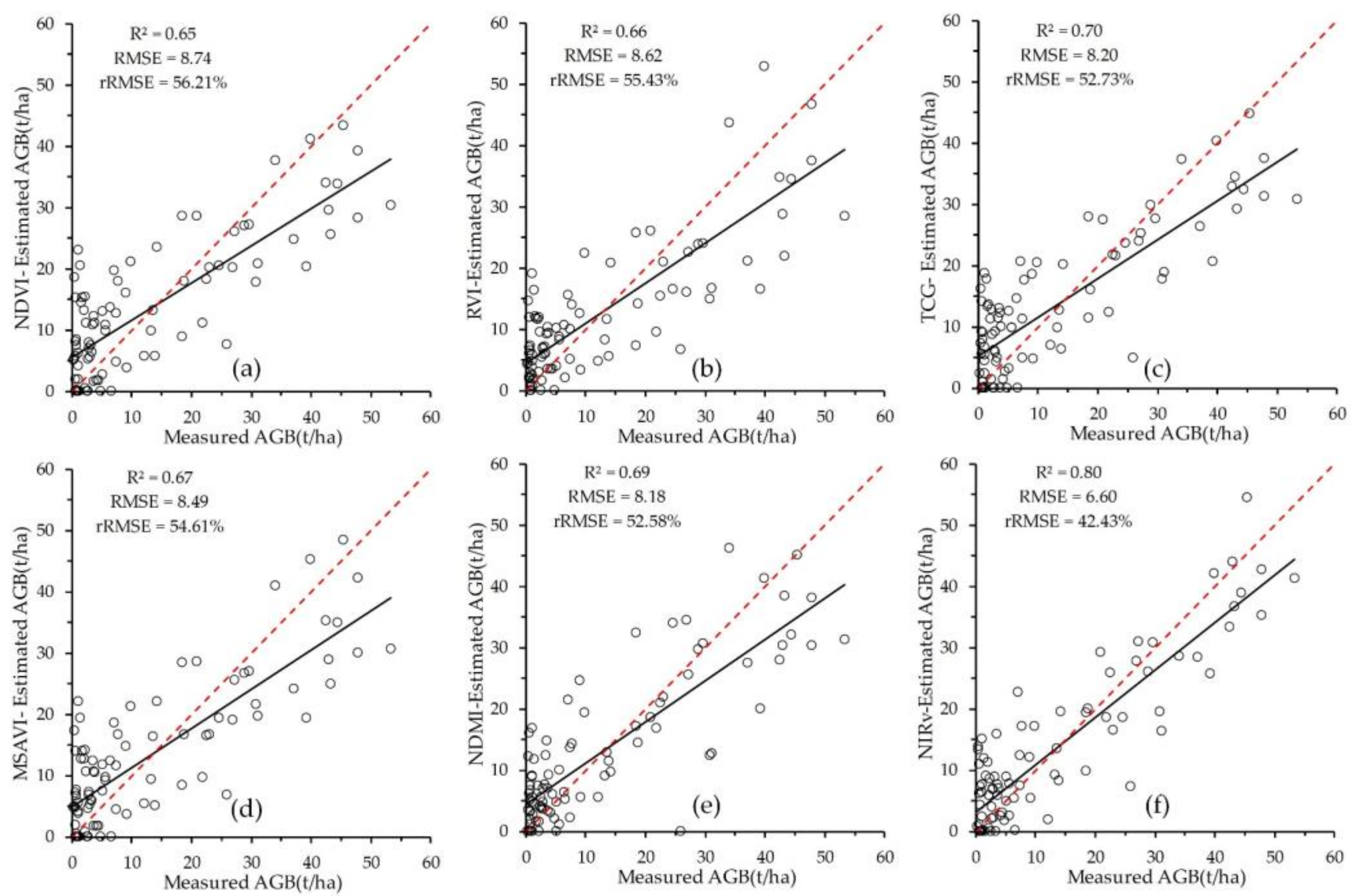
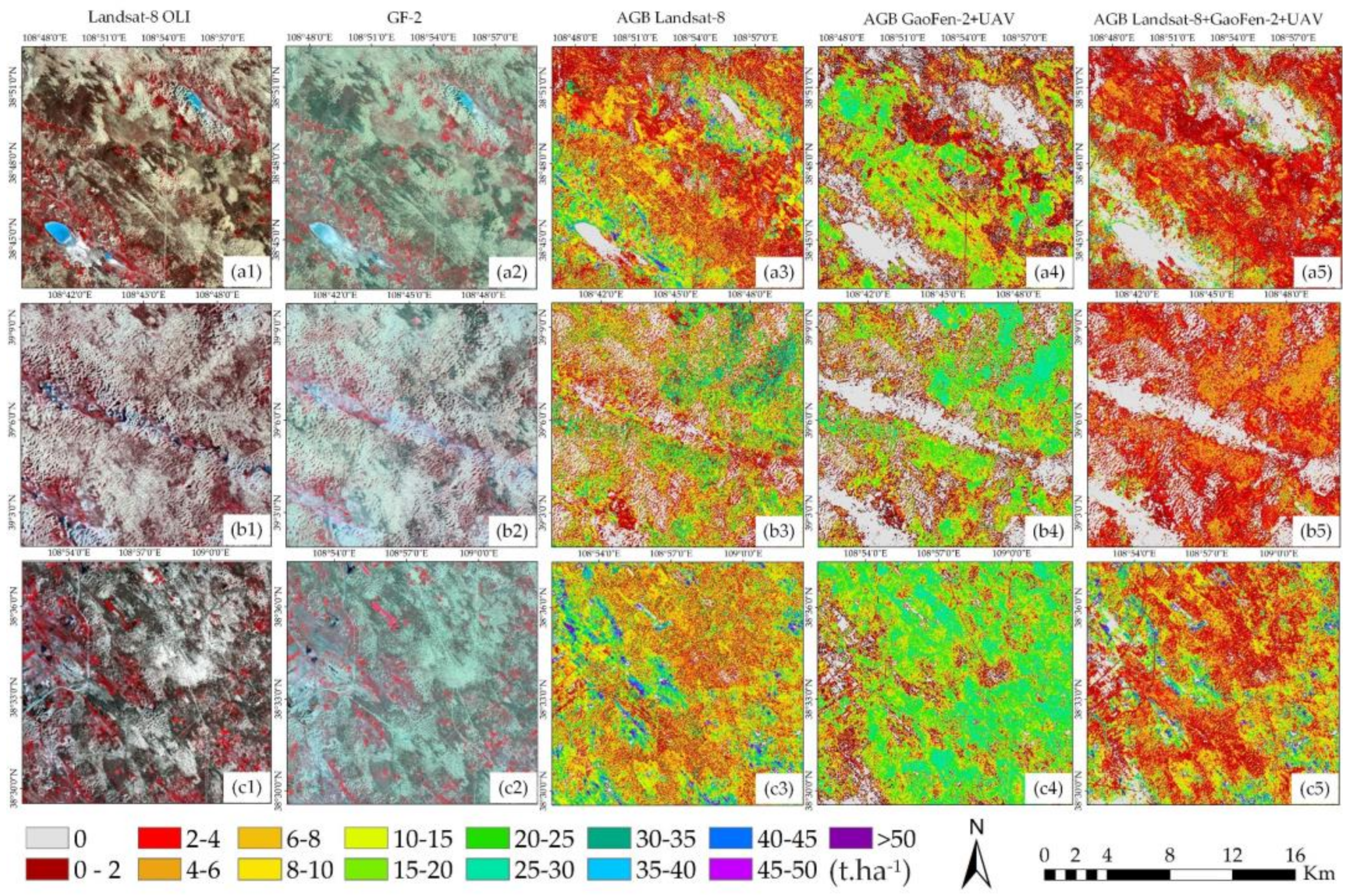
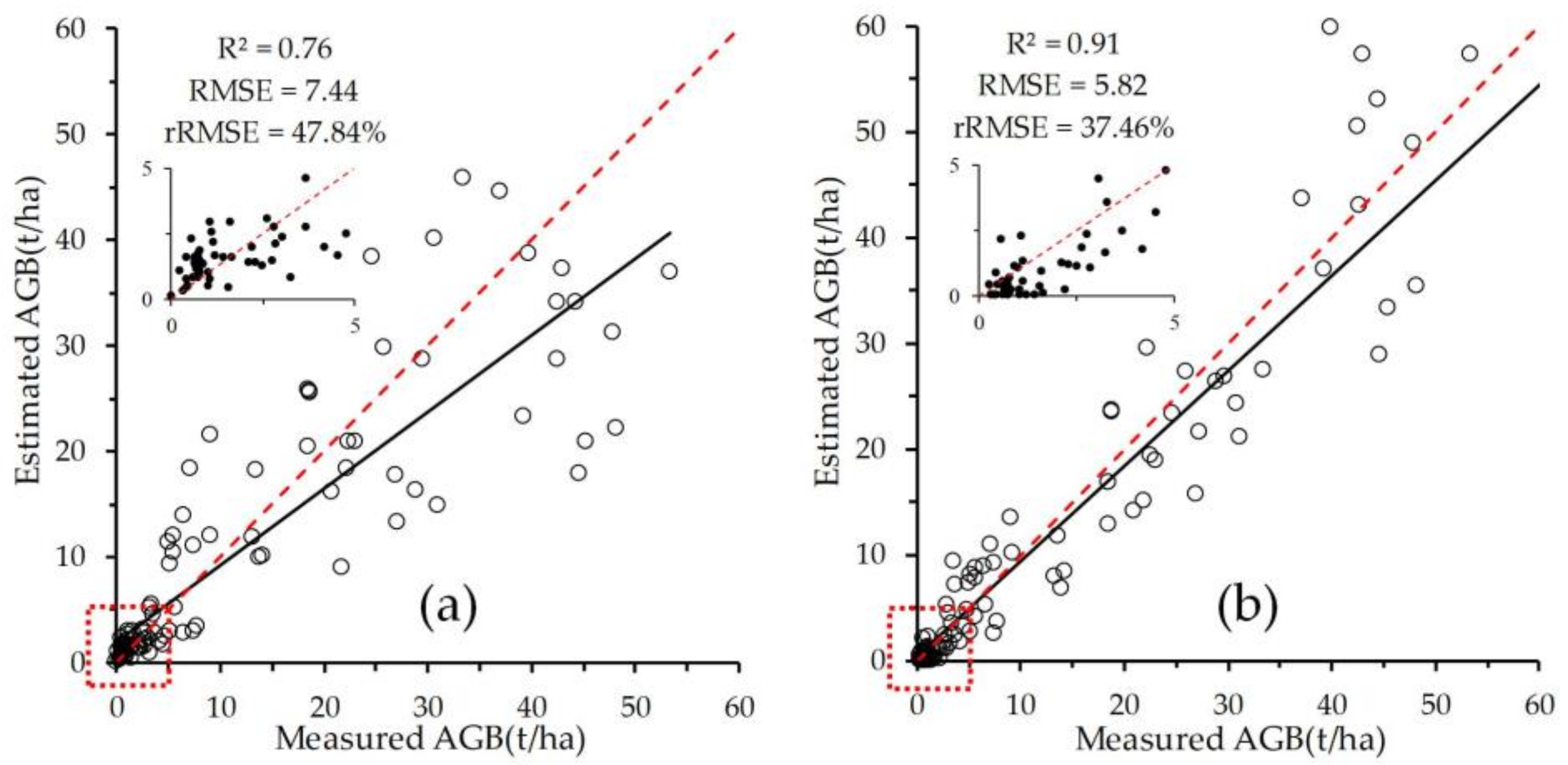
4.4. Accuracy Assessment of the Woody AGB Estimations Obtained Using Different Modeling Schemes

In this study, the plot-level woody AGBs of 102 plots were calculated using the plot-level woody AGB models derived from the Landsat-8 and UAV images (in Section 4.2) and the woody and herbaceous vegetation coverages derived from the GaoFen-2 (in Section 4.3). Consequently, the accuracy metrics of R2, root mean square error (RMSE) and relative root mean square error (rRMSE) were employed to evaluate the performances of the VI-AGB models using only Landsat-8 imagery, the woody cover-AGB model using a combination of GaoFen-2 and UAV images, and the stratification-based VI-AGB models using a combination of Landsat-8, GaoFen-2, and UAV images (Figure 8, Figure 9 and Figure 10).
The woody AGB estimated using the woody coverage AGB model had a poor performance, with R2, RMSE and rRMSE values of 0.22, 14.98 t∙ha1, and 96.31%, respectively. As Figure 8 shows, the AGB of the low woody vegetation (e.g., shrubs) was overestimated and the AGB of the high woody vegetation (e.g., trees) was underestimated. This indicates that the woody coverage cannot perfectly explain the variation in the woody AGB in a sparse forest containing a mixture of trees and shrubs. The accuracy assessment of the AGB estimates obtained using the different VI-AGB models (Figure 9) show that the different VIs have different performances with regard to the woody AGB estimation. The NIRv-AGB model performed the best among the six VIs used in this study, with R2, RMSE and rRMSE values of 0.72, 7.91 t∙ha−1, and 50.89%, respectively. In contrast, the NDVI-AGB model had the poorest performance, with R2, RMSE and rRMSE values of 0.53, 10.18 t∙ha−1, and 65.44%, respectively, which demonstrates the implication of selecting the optimal VI to estimate the woody AGB. The abilities of the different VIs to explain the woody AGB variation in the sparse mixed forest were ranked as follows: NIRv > NDMI > TCG > MSAVI > RVI > NDVI.
The woody AGB estimated using the stratification-based VI-AGB models (Figure 10) indicate that the NIRv-AGB model still performed the best (R2 of 0.72, RMSE of 7.91 t∙ha−1, and rRMSE of 50.89%), while the NDVI-AGB model had the poorest performance (R2 of 0.53, RMSE of 10.18 t∙ha−1 and rRMSE of 65.44%). Comparative analysis of Figure 8, Figure 9 and Figure 10 revealed that all VI-AGB models performed better than the woody coverage-AGB model in terms of estimating the woody AGB in the sparse mixed forest, and the accuracies of the VI-AGB models can be significantly improved by applying the stratified modeling strategy and by considering the heterogeneity of the background of the woody vegetation (green herbaceous vegetation coverage). However, the sensitivities of the different VIs to the herbaceous vegetation coverage are different. Among them, the NIRv-AGB model was the most sensitive to the herbaceous vegetation, with the RMSE (rRMSE) decreasing from 7.91 t∙ha−1 (50.89%) (non-stratification) to 6.60 t∙ha−1 (42.43%) (stratification). The NDMI-AGB model was the least sensitive to the herbaceous vegetation, with the RMSE (rRMSE) decreasing from 8.90 t∙ha−1 (57.24%) (non-stratification) to 8.18 t∙ha−1 (52.58%) (stratification). The sensitivities of the different VI-AGB models to the background of the herbaceous vegetation were ranked as follows: NIRv > TCG > NDVI > MSAVI > RVI > NDMI.
The woody AGB derived using the woody coverage-AGB model, the NIRv-AGB model, and the stratification-based NIRv-AGB model in three subregions are shown in Figure 11. As can be seen, the woody coverage-AGB model using the GaoFen-2 and UAV images significantly overestimated the woody AGB (especially for 15–20 t∙ha−1) in the area covered by numerous dwarf shrubs, while the AGB of the high trees were underestimated. The woody AGB was easily overestimated by the NIRv-AGB model using only Landsat-8 imagery due to the mixed spectral signal contributed by the woody and green herbaceous canopies. The estimates of the stratification-based NIRv-AGB model using a combination of Landsat-8, GaoFen-2, and UAV images are more consistent with actual spatial distribution of the woody trees and shrubs.

5. Discussion

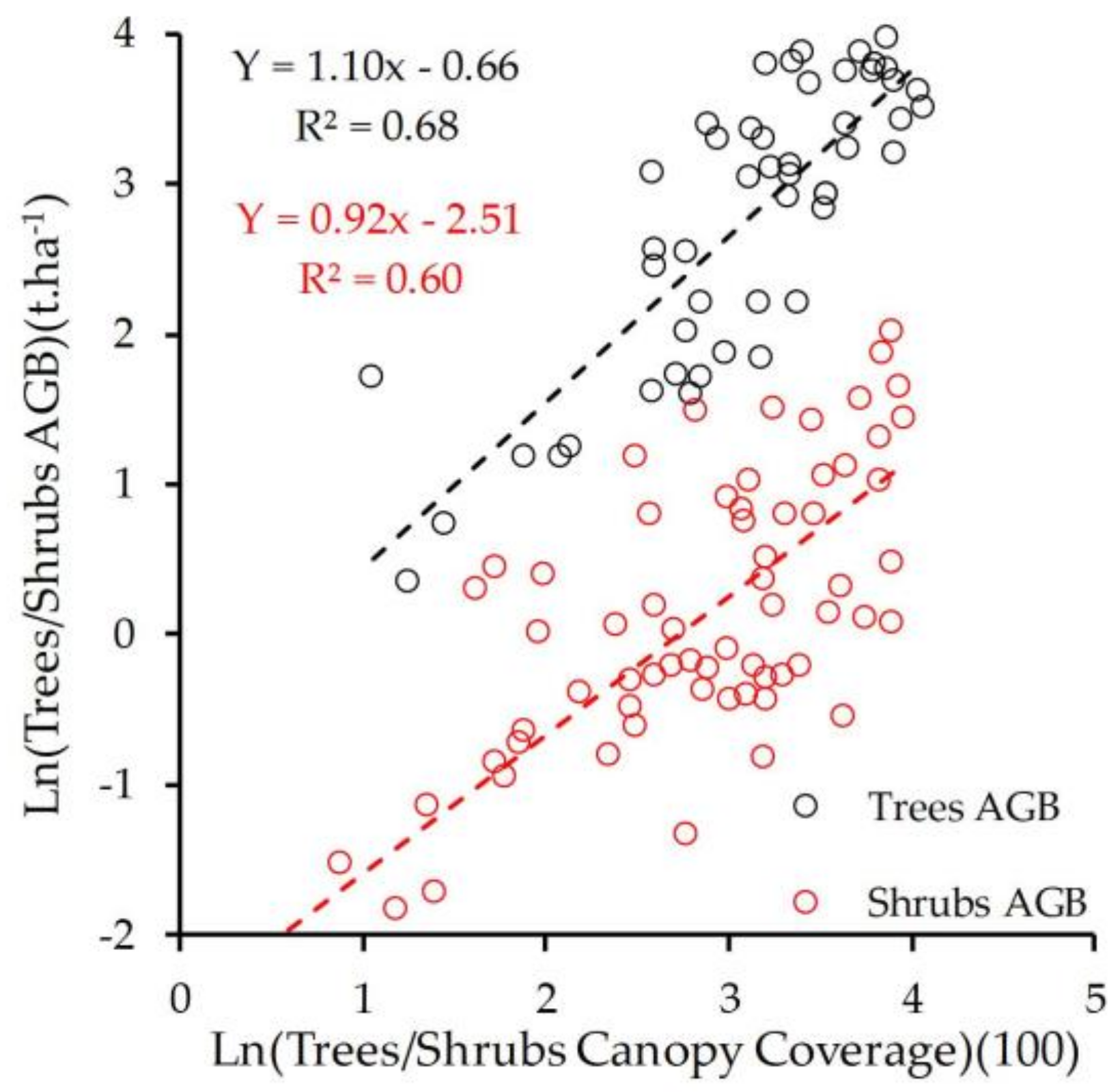
5.1. Applicability of the Woody Cover-AGB Model to Sparse Mixed Forests

It has been reported that the woody canopy coverage derived from high-resolution aerial or satellite imagery has a promising potential for accurately estimating the woody AGB of sparse woody vegetation in arid areas [6,30,47,48]. However, in this study, the accuracy of the woody coverage-AGB model was very low for the sparse mixed forest (Figure 8). In order to analyze the underlying causes of the low accuracy of the woody coverage-AGB model, we developed different plot-level woody coverage-AGB models stratified based on two woody vegetation types (trees and shrubs) and five woody species (Populus alba, Salix matsudana, Pinus tabuliformis, Artemisia ordosida, and Caragana korshinskii). Then, the plot-level woody AGBs of all of the plots were calculated using stratification-based models under two schemes. The accuracy assessment of the stratification-based models is shown in Figure 12.
By comparing Figure 8 and Figure 12, it can be seen that compared with the woody coverage-AGB model that does not consider the woody vegetation types (RMSE = 14.98 t∙ha−1 and rRMSE = 96.31%), the estimation uncertainties of the woody coverage-AGB models stratified based on two woody vegetation types (RMSE = 7.44 t∙ha−1 and rRMSE = 47.84%) and the woody coverage-AGB models stratified based on five woody species (RMSE = 5.82 t∙ha−1 and rRMSE = 37.46%) were 50.32 and 61.1% lower, respectively. This demonstrates that the woody coverage-AGB model is significantly more sensitive to the heterogeneity of woody vegetation types, and the finer the classification of the woody vegetation is, the more accurate the estimation of the woody AGB is.
To explain the impact of woody vegetation types on the accuracy of woody coverage-AGB model, we compared the relationship between canopy coverage and woody AGB of the trees and shrubs, as illustrated in the Figure 13, and it was found that the woody coverage-AGB regression models for trees and shrubs are significantly different, which could be explained by the divergent ratios of the crown area to the canopy height of trees and shrubs [32]. For example, although the canopy coverages derived from crown area of trees and shrubs are same, the AGB of them could be significantly different as a result from difference in height of trees and shrubs.

5.2. Applicability of the Landsat VI-AGB Model to Sparse Mixed Forest

According to the physical principle of the radiative transfer process [49], the leaf area index (LAI) rather than the canopy coverage is the critical structural canopy parameter affecting the spectral signals acquired by satellite sensors, so the VI-AGB model reflects the intrinsic biophysical response relationship between the LAI and the AGB of woody vegetation [1,50]. Because the relationship between the LAI and AGB is less sensitive to woody vegetation types than the relationship between the woody coverage and the AGB, VI-AGB model for mixed tree-shrub forest has a much lower sensitivity to vegetation types than the woody coverage-AGB model. This could explain why the accuracy of the woody coverage-AGB model (Figure 8) was lower than that of the VI-AGB models (Figure 9 and Figure 10).
The NIRv has been found to be strongly correlated with the gross primary productivity (GPP) in a large number of studies [51,52,53,54], and we found that the correlation between the NIRv and the sparse woody AGB is also better than those of the other vegetation indices, which may be due to the strong ability of the NIRv to characterize canopy structures and reduce the impact of the background on the spectral signal of the woody canopy [55]. However, because the spectral signal of the woody canopy can be easily affected by the background (e.g., green herbaceous vegetation) at the 30 m scale in a sparse forest, the heterogeneity of the background of the woody vegetation can seriously affect the estimation accuracy of the VI-AGB model. Figure 9 shows that the sensitivities of the different VIs to the heterogeneity of the background are different. Because the NIRv is the product of the NDVI and the NIR [56], and the NDVI is more sensitive to the greenness of the background, the accuracy of the woody AGB estimated using the NDVI and NIRv will be significantly affected by green herbaceous vegetation. Since the NDMI is less sensitive to herbaceous vegetation because the variation in the leaf water content of herbaceous vegetation in arid areas is relatively low [3], the impact of the herbaceous vegetation coverage on the estimation accuracy of the NDMI-AGB model is very low.

5.3. Potential of Using High-Resolution Remote Sensing Images for AGB Estimation of Sparse Mixed Forest

In this study, the canopy of trees, shrubs, and herbaceous vegetation and bare soil was accurately classified using the object-based SVM classification method based on a UAV RGB image, with an average overall accuracy and kappa coefficient of 93.44% and 0.91, respectively, which indicates that super high-resolution UAV images can replace time-consuming and labor-intensive manual field surveys and obtain highly effectively canopy structural parameters in sparsely vegetated area. Other studies have also shown that high-resolution UAV inversion of vegetation canopy coverage has high accuracy and has the potential to replace field surveys [6,57].
Because the coverage area of UAV image is very limited, the vegetation canopy coverage over a large area cannot be obtained directly from UAV images; however, the retrievals from the UAV image can be used to improve the canopy coverage of woody and herbaceous vegetation derived from high-resolution satellite images (GaoFen-2) with larger coverage areas, which is very helpful in determining the accurate fractional vegetation coverage over a large area. UAV images serve as a bridge connecting field measurements and satellite images.
For other studies on remote sensing inversion AGB in dryland areas, they all extracted canopy coverage with high-resolution images in homogeneous sparse trees/shrubs areas to construct canopy coverage-AGB models [32,37,38]. However, the experimental results of this study indicated that the inversion accuracy of canopy coverage-AGB model would be reduced in sparse tree-shrub mixed forest. The surface background of herbaceous vegetation affects AGB estimation accuracy of VI-AGB models in dryland areas [30]. From comparing the different common AGB inversion methods, the stratification-based VI-AGB model was proposed to improve the accuracy of biomass inversion in sparse mixed forests in this study. This study demonstrates that the woody AGB estimated using VI-AGB models stratified based on different levels of herbaceous coverage is significantly improved (Figure 10). This can be explained by the lower sensitivity of VIs to the variations in an herbaceous vegetation background with a specific level of herbaceous coverage [6]. Therefore, high-resolution information about the vegetation canopy derived from aerial and satellite images has a great potential for improving the woody AGB estimation of sparse mixed forests associated with highly heterogeneous woody vegetation types and background types. In addition, we also compared the AGB estimated by our study and global AGB product [15,39], and it was found that the AGB from global product was zero in the study area, which indicates that it is a challenge to estimate AGB in dryland ecosystem for global product.

5.4. Uncertainty Analysis

The plot-level woody AGB used in this study was calculated using the allometric equations presented in previous studies. This could introduce some uncertainties into the absolute value of the woody AGB, but systematic deviations in the woody AGB will not affect the comparison of the relative relationship of the accuracies of the different woody AGB estimation methods [30]. Although the classification accuracy of the object-based and pixel-based machine learning algorithm is very high, the classification error induced by the sun illumination, shadow effect, and sample selection still inevitably affect the accuracy of the final woody AGB estimates. The sparse and dwarf shrubs cannot be accurately identified by remote sensing data due to the low spectral signal acquired by the sensor. The spatial mismatch between the field plot measurements and Landsat-8 satellite observations could lead to some uncertainties in the VI-AGB models; however, the plot-level VI obtained using the weighted average method was proposed in this study to partly overcome this problem.

6. Conclusions

In this study, a woody coverage-AGB model using Gaofen-2 and UAV images, VIs-AGB model using Landsat-8 image and a VIs-AGB model stratified by herbaceous vegetation coverage using landsat-8, Gaofen-2 and UAV images were employed to estimate the woody AGB of sparse mixed forest over a dryland ecosystem, respectively.
It can be concluded that the woody and herbaceous canopy can be accurately identified using the object-based classification based on an UAV RGB image; therefore, UAV observation has a great potential to replace time-consuming and labor-intensive manual field survey in sparsely vegetated areas, and it can be used to improve the canopy coverage of woody and herbaceous vegetation derived from high-resolution satellite images. UAV images serve as a critical bridge between field measurements and satellite observations. In addition, the accuracy of the woody coverage-AGB model cannot be satisfied until the woody vegetation types (e.g., trees and shrubs) are considered. VIs-AGB models performed better for the sparse mixed forest when vegetation types were not clear; however, the accuracy of VIs-AGB models could be easily affected by heterogeneity of the herbaceous vegetation. Last but not least, a VIs-AGB model stratified by herbaceous vegetation coverage is a practical and easy-to-use method to improve the estimation accuracy of woody AGB of sparse mixed forest using remote sensing data over a large area, and the NIRv perform better than other five commonly used VIs in this study on the estimation of woody AGB.
However, the present study requires further investigation. More samples databases and deep-learning algorithms such as convolutional neural networks (CNN) are needed to improve the classification of the UAV images. In addition, the physical response relationship between the spectral characteristics and the woody AGB should be further researched using a combination of spectral mixture analysis and a radiative transfer model in the future. Microwave and LiDAR data in the future mission can also be combined with optical data to improve the accuracy of the woody AGB estimation over dryland ecosystems.

Author Contributions

Y.S. performed the data interpretation, processing and wrote the first draft of the manuscript. Z.W. gave constructive suggestions on the design and modification of the manuscript. L.L., D.P. and C.L. also helped process the data in this paper. P.X. helped edit the manuscript prior to submission. All authors have read and agreed to the published version of the manuscript.

Funding

This research was funded by the National Natural Science Foundation of China (41701509, 41671407), Special Research Fund of the YRIHR (HKY-JBYW-2020-09), Program of Youth Backbone Teachers in Henan province of China (2019GGJS059) and Young Elite Scientist Sponsorship by CAST (2017QNRC023).

Data Availability Statement

The data presented in this study are available on request from the corresponding author for research purposes.

Acknowledgments

We gratefully thank the anonymous reviewers for their critical comments and constructive suggestions on the manuscript.

Conflicts of Interest

The authors declare no conflict of interest.

References

  1. Xiao, J.F.; Frederic, C.; Cecile, G.; Luis, G.; Jeffrey, A.H. Remote sensing of the terrestrial carbon cycle: A review of advances over 50 years. Remote Sens. Environ. 2019, 233, 1383. [Google Scholar] [CrossRef]
  2. Chen, J. Carbon neutrality: Toward a sustainable future. Innovation 2021, 2, 100127. [Google Scholar] [CrossRef] [PubMed]
  3. Smith, W.K.; Dannenberg, M.P.; Yan, D.; Herrmann, S.; Barnes, M.L.; Barron-Gafford, G.A. Remote sensing of dryland ecosystem structure and function: Progress, challenges, and opportunities. Remote Sens. Environ. 2019, 233, 1401. [Google Scholar] [CrossRef]
  4. Zhang, Y.; Peng, C.H.; Li, W.D.; Tian, L.X.; Zhu, Q.; Chen, H.; Fang, X.Q. Multiple afforestation programs accelerate the greenness in the ‘Three North’ region of China from 1982 to 2013. Ecol. Indic. 2016, 61, 404–412. [Google Scholar] [CrossRef]
  5. Liu, L.Y. Opportunities of Mapping Forest Carbon Stock and its Annual Increment Using Landsat Time-Series Data. Geoinformatics Geostat. Overv. 2016, 4, 151. [Google Scholar] [CrossRef] [Green Version]
  6. Guo, Z.; Wang, T.; Liu, S.L.; Kang, W.P.; Chen, X. Biomass and vegetation coverage survey in the Mu Us sandy land-based on unmanned aerial vehicle RGB images. Int. J. Appl. Earth Obs. Geoinf. 2021, 94, 2239. [Google Scholar] [CrossRef]
  7. Main-Knorn, M.; Cohen, W.B.; Kennedy, R.E.; Grodzki, W.; Pflugmacher, D. Monitoring coniferous forest biomass change using a Landsat trajectory-based approach. Remote Sens. Environ. 2013, 139, 277–290. [Google Scholar] [CrossRef]
  8. Liu, L.Y.; Peng, D.L.; Wang, Z.H. Improving artificial forest biomass estimates using afforestation age information from time series Landsat stacks. Environ. Monit. Assess. 2014, 186, 7293–7306. [Google Scholar] [CrossRef]
  9. Peng, D.L.; Zhang, H.L.; Liu, L.Y. Estimating the Aboveground Biomass for Planted Forests Based on Stand Age and Environmental Variables. Remote Sens. 2019, 11, 2270. [Google Scholar] [CrossRef] [Green Version]
  10. Ni, W.J.; Zhang, Z.Y.; Sun, G.Q.; Sun, Y.F.; He, Y.T. The Penetration Depth Derived from the Synthesis of ALOS/PALSAR InSAR Data and ASTER GDEM for the Mapping of Forest Biomass. Remote Sens. 2014, 6, 7307–7319. [Google Scholar] [CrossRef] [Green Version]
  11. Latifi, H.; Fassnacht, F.E.; Hartig, F.; Berger, C.; Hernández, J.; Corvalán, P. Stratified aboveground forest biomass estimation by remote sensing data. Int. J. Appl. Earth Obs. Geoinf. 2015, 38, 229–241. [Google Scholar] [CrossRef]
  12. Liu, X.; Yang, L.; Liu, Q.H.; Li, J. Review of forest above ground biomass inversion methods based on remote sensing technology. J. Remote Sens. 2015, 19, 62–74. (In Chinese) [Google Scholar]
  13. Lu, D.; Chen, G.; Wang, Q.; Liu, L.; Li, G.; Moran, E. A survey of remote sensing-based aboveground biomass estimation methods in forest ecosystems. Int. J. Digit. Earth 2016, 9, 63–105. [Google Scholar] [CrossRef]
  14. Markus, T.; Neumann, T.; Martino, A.; Abdalati, W.; Brunt, K.; Csatho, B.; Farrell, S. The Ice, Cloud, and land Elevation Satellite-2 (ICESat-2): Science requirements, concept, and implementation. Remote Sens. Env. 2017, 190, 260–273. [Google Scholar] [CrossRef]
  15. Le Toan, T.; Quegan, S.; Davidson, M.; Balzter, H.; Paillou, P.; Papathanassiou, K. The BIOMASS mission: Mapping global forest biomass to better understand the terrestrial carbon cycle. Remote Sens. Environ. 2011, 115, 2850–2860. [Google Scholar] [CrossRef] [Green Version]
  16. Rosen, P.; Hensley, S.; Shaffer, S.; Edelstein, W.; Kim, Y.; Kumar, R.; Misra, T. An update on the NASA-ISRO dual-frequency dbf SAR(NISAR) mission. In 2016 IEEE International Geoscience and Remote Sensing Symposium; IEEE: New York, NY, USA, 2016; pp. 2106–2108. [Google Scholar]
  17. Todd, S.W.; Hoffer, R.M.; Milchunas, D.G. Biomass estimation on grazed and ungrazed rangelands using spectral indices. Int. J. Remote Sens. 1998, 19, 427–438. [Google Scholar] [CrossRef]
  18. Boyd, D.S.; Foody, G.M.; Ripple, W.J. Evaluation of approaches for forest cover estimation in the Pacific Northwest, USA, using remote sensing. Appl. Geogr. 2002, 22, 375–392. [Google Scholar] [CrossRef]
  19. Zhang, L.; Wylie, B.; Loveland, T.; Fosnight, E.; Tieszen, L.L.; Ji, L.; Gilmanov, T. Evaluation and comparison of gross primary production estimates for the Northern Great Plains grasslands. Remote Sens. Environ. 2006, 106, 173–189. [Google Scholar] [CrossRef] [Green Version]
  20. Tan, K.; Piao, S.L.; Peng, C.H.; Fang, J.Y. Satellite-based estimation of biomass carbon stocks for northeast China’s forests between 1982 and 1999. Forest Ecol. Manag. 2006, 240, 114–121. [Google Scholar] [CrossRef]
  21. Yan, F.; Wu, B.; Wang, Y.J. Estimating spatiotemporal patterns of aboveground biomass using Landsat TM and MODIS images in the Mu Us Sandy Land, China. Agric. Forest Meteorol. 2015, 200, 119–128. [Google Scholar] [CrossRef]
  22. LI, F.; Zeng, Y.; Luo, J.H.; Ma, R.H.; Wu, B.F. Modeling grassland aboveground biomass using a pure vegetation index. Ecol. Indic. 2016, 62, 279–288. [Google Scholar] [CrossRef]
  23. Zhao, P.P.; Lu, D.S.; Wang, G.X.; Wu, C.P.; Huang, Y.J.; Yu, S.Q.; Tomppo, E.; McRorberts, B.E. Examining Spectral Reflectance Saturation in Landsat Imagery and Corresponding Solutions to Improve Forest Aboveground Biomass Estimation. Remote Sens. 2016, 8, 469. [Google Scholar] [CrossRef] [Green Version]
  24. Rahman, S.L.; Nichol, J.E. Improved forest biomass estimates using ALOS AVNIR-2 texture indices. Remote Sens. Environ. 2010, 115, 968–977. [Google Scholar]
  25. Shoshany, M.; Karnibad, L. Mapping shrubland biomass along Mediterranean climatic gradients: The synergy of rainfall-based and NDVI-based models. Int. J. Remote Sens. 2011, 32, 9497–9508. [Google Scholar] [CrossRef]
  26. Chen, Q.; Vaglio, L.G.; Battles, J.J.; Saah, D. Integration of airborne lidar and vegetation types derived from aerial photography for mapping aboveground live biomass. Remote Sens. Environ. 2012, 121, 108–117. [Google Scholar] [CrossRef]
  27. Feng, Y.Y.; Lu, D.S.; Chen, Q.; Keller, M.; Moran, E.; Nara, D.S.; Luis, B.E.; Batistella, M. Examining Effective Use of Data Sources and Modeling Algorithms for Improving Biomass Estimation in a Moist Tropical Forest of the Brazilian Amazon; Taylor & Francis: Oxfordshire, UK, 2017; Volume 10, pp. 996–1016. [Google Scholar]
  28. Jiang, X.D.; Li, G.Y.; Lu, D.S.; Chen, E.X.; Wei, X.L. Stratification-Based Forest Aboveground Biomass Estimation in a Subtropical Region Using Airborne Lidar Data. Remote Sens. 2020, 12, 1101. [Google Scholar] [CrossRef] [Green Version]
  29. Zandler, H.; Brenning, A.; Samimi, B. Quantifying dwarf shrub biomass in an arid environment: Comparing empirical methods in a high dimensional setting. Remote Sens. Environ. 2015, 158, 140–155. [Google Scholar] [CrossRef]
  30. Wang, Z.H.; Gary, N.B.; Liu, L.Y.; Peter, A.C.; Peng, D.L. Estimating woody above-ground biomass in an arid zone of central Australia using Landsat imagery. J. Appl. Remote Sens. 2015, 9, 096036. [Google Scholar] [CrossRef]
  31. Fu, T.; Pang, Y.; Huang, Q.N. Prediction of subtropical forest parameters using airborne laser scanner. Natl. Remote Sens. Bull. 2011, 15, 1092–1104. (In Chinese) [Google Scholar]
  32. Wang, Z.H.; Liu, L.Y.; Peng, D.L.; Liu, X.J.; Zhang, S. Estimating woody aboveground biomass in an area of agroforestry using airborne light detection and ranging and compact airborne spectrographic imager hyperspectral data: Individual tree analysis incorporating tree species information. J. Appl. Remote Sens. 2016, 10, 036007. [Google Scholar] [CrossRef]
  33. Lato, M.; Dong, P.; Chen, Q. LiDAR Remote Sensing and Applications. Math. Geosci. 2019, 51, 1874–8961. [Google Scholar]
  34. Leboeuf, A.; Beaudoin, A.; Fournier, R.A.; Guindon, L.; Luther, J.E.; Lambert, M.C. A shadow fraction method for mapping biomass of northern boreal black spruce forests using QuickBird imagery. Remote Sens. Environ. 2007, 110, 488–500. [Google Scholar] [CrossRef]
  35. Dube, T.; Gara, T.W.; Mutanga, O. Estimating forest standing biomass in savanna woodlands as an indicator of forest productivity using the new generation WorldView-2 sensor. Geocarto Int. 2018, 33, 178–188. [Google Scholar] [CrossRef]
  36. Maack, J.; Kattenborn, T.; Fassnacht, F.E.; Enßle, F.; Hernández, J. Modeling forest biomass using Very-High-Resolution data—Combining textural, spectral and photogrammetric predictors derived from spaceborne stereo images. Eur. J. Remote Sens. 2015, 48, 245–261. [Google Scholar] [CrossRef] [Green Version]
  37. Suganuma, H.; Abe, Y. Taniguchi, M.; Utsugi, H.; Kojima, T.; Yamada, K. Stand biomass estimation method by canopy coverage for application to remote sensing in an arid area of Western Australia. Forest Ecol. Manag. 2005, 222, 75–87. [Google Scholar] [CrossRef]
  38. Ozdemir, I. Estimating stem volume by tree crown area and tree shadow area extracted from pan-sharpened Quickbird imagery in open Crimean juniper forests. Int. J. Remote Sens. 2008, 29, 5643–5655. [Google Scholar] [CrossRef]
  39. Santoro, M.; Cartus, O.; Mermoz, S.; Bouvet, A.; Le Toan, T.; Carvalhais, N. A detailed portrait of the forest aboveground biomass pool for the year 2010 obtained from multiple remote sensing observations. Geophys. Res. Abstr. 2018, 20, 18932. [Google Scholar]
  40. Zhao, A.Z.; Zhang, A.B.; Lu, C.Y.; Wang, D.L.; Wang, H.F.; Liu, H.X. Spatiotemporal variation of vegetation coverage before and after implementation of Grain for Green Program in Loess Plateau, China. Ecol. Eng. 2017, 104, 13–22. [Google Scholar] [CrossRef]
  41. Liu, Z.J.; Liu, Y.S.; Li, Y.R. Anthropogenic contributions dominate trends of vegetation cover change over the farming-pastoral ecotone of northern China. Ecol. Indic. 2018, 95, 370–378. [Google Scholar] [CrossRef]
  42. Guo, Z.C.; Liu, S.L.; Kang, W.P.; Chen, X.Z.; Xue, Q. Change trend of vegetation coverage in the mu us sandy region from 2000 to 2015. Desert Res. 2018, 21, 19–37. (In Chinese) [Google Scholar]
  43. Li, H.K. Estimation and Evaluation of Forest Biomass Carbon Storage in China; China Forestry Press: Beijing, China, 2010; Volume 5, pp. 52–59. (In Chinese) [Google Scholar]
  44. Harikumar, A.; Bovolo, F.; Bruzzone, L. An internal crown geometric model for conifer species classification with high-density lidar data. IEEE Trans. Geosci. Remote Sens. 2017, 55, 2924–2940. [Google Scholar] [CrossRef]
  45. Chen, C.; Fu, J.Q.; Zhang, S.; Zhao, X. Coastline information extraction based on the tasseled cap transformation of Landsat-8 OLI images. Estuar. Coast. Shelf Sci. 2019, 217, 281–291. [Google Scholar] [CrossRef]
  46. Gilmore, P.R.; Millones, M. Death to Kappa: Birth of quantity disagreement and allocation disagreement for accuracy assessment. Int. J. Remote Sens. 2011, 32, 4407–4429. [Google Scholar]
  47. Eisfelder, C.; Kuenzer, C.; Dech, S. Derivation of biomass information for semi-arid areas using remote-sensing data. Int. J. Remote Sens. 2012, 33, 2937–2984. [Google Scholar] [CrossRef]
  48. Zhang, C.; Lu, D.S.; Chen, X.; Zhang, Y.M.; Maisupova, B.; Tao, Y. The spatiotemporal patterns of vegetation coverage and biomass of the temperate deserts in Central Asia and their relationships with climate controls. Remote Sens. Environ. 2016, 175, 271–281. [Google Scholar] [CrossRef]
  49. He, L.; Li, A.N.; Yin, G.F.; Nan, X.; Bian, J.H. Retrieval of Grassland Aboveground Biomass through Inversion of the PROSAIL Model with MODIS Imagery. Remote Sens. 2019, 11, 1597. [Google Scholar] [CrossRef] [Green Version]
  50. Zhang, X.Y.; Kondragunta, S. Estimating forest biomass in the USA using generalized allometric models and MODIS land products. Geophys. Res. Lett. 2006, 33, L09402. [Google Scholar] [CrossRef] [Green Version]
  51. Luo, Y.P.; El-Madany, T.S.; Filippa, G.; Ma, X.L.; Ahrens, B.; Carrara, A. Using Near-Infrared-Enabled Digital Repeat Photography to Track Structural and Physiological Phenology in Mediterranean Tree–Grass Ecosystems. Remote Sens. 2018, 10, 1293. [Google Scholar] [CrossRef] [Green Version]
  52. Fernández-Martínez, M.; John, G.; Hmimina, G.; Filella, L.; Balzarolo, M.; Benjamin, S. Monitoring Spatial and Temporal Variabilities of Gross Primary Production Using Maiac Modis Data. Remote Sens. 2019, 11, 874. [Google Scholar] [CrossRef] [Green Version]
  53. Huang, X.J.; Xiao, J.F.; Ma, M.G. Evaluating the Performance of Satellite-Derived Vegetation Indices for Estimating Gross Primary Productivity Using FLUXNET Observations across the Globe. Remote Sens. 2019, 11, 1823. [Google Scholar] [CrossRef] [Green Version]
  54. Hinojo-Hinojo, C.; Michael, L.G. Plant Traits Help Explain the Tight Relationship between Vegetation Indices and Gross Primary Production. Remote Sens. 2020, 12, 1405. [Google Scholar] [CrossRef]
  55. Grayson, B.; Christopher, B.F.; Joseph, A.B. Canopy near-infrared reflectance and terrestrial photosynthesis. Sci. Adv. 2017, 3, e1602244. [Google Scholar]
  56. Badgley, G.; Anderegg, L.; Berry, J.A. Terrestrial gross primary production: Using NIRV to scale from site to globe. Glob. Chang. Biol. 2019, 25, 3731–3740. [Google Scholar] [CrossRef] [PubMed]
  57. Wang, H.; Han, D.; Mu, Y. Landscape-level vegetation classification and fractional woody and herbaceous vegetation cover estimation over the dryland ecosystems by unmanned aerial vehicle platform. Agric. For. Meteorol. 2019, 278, 107665. [Google Scholar] [CrossRef]
Figure 1. Spatial distribution of the observations from the field survey and the Landsat-8, GaoFen-2, and UAV images of the Mu Us Sandy Land.
Remotesensing 13 04859 g001
Figure 2. Overall workflow of the woody AGB estimation for a sparse mixed forest (canopy coverage represents the ratio of vegetation canopy area to the total area of the plot).
Remotesensing 13 04859 g002
Figure 3. Schematic diagram of the method of obtaining the plot-level Landsat VI using the weighted average method.
Remotesensing 13 04859 g003
Figure 4. (a1,b1,c1) UAV RGB images and (a2,b2,c2) their object-based classification images for three subregions in the study area.
Remotesensing 13 04859 g004
Figure 5. Quantile statistics of the accuracy indicators of the UAV RGB image classifications of all field plots: (a) overall accuracy and kappa coefficient, (b) producer’s accuracy and user’s accuracy.
Remotesensing 13 04859 g005
Figure 6. Pixel-based SVM classification using GaoFen-2 image in three subregions (ac) of the study area.
Remotesensing 13 04859 g006
Figure 7. Calibration models for woody and herbaceous coverage derived from GaoFen-2 imagery: (a) herbaceous coverage calibration model, and (b) woody coverage calibration model.
Remotesensing 13 04859 g007
Figure 8. Accuracy assessment of the estimated woody AGB obtained using the woody coverage-AGB model in the scheme 1. The black line represents the regression line, the red line represents the 1:1 line.
Remotesensing 13 04859 g008
Figure 9. Accuracy assessment of the woody AGB estimated using the VI-AGB models for the (a) NDVI; (b) RVI; (c) TCG; (d) MSAVI; (e) NDMI, and (f) NIRv in scheme 2. The black line represents the regression line, the red line represents the 1:1 line.
Remotesensing 13 04859 g009
Figure 10. Accuracy assessment of the woody AGB estimated using the stratification-based VI-AGB models for the (a) NDVI; (b) RVI; (c) TCG; (d) MSAVI; (e) NDMI, and (f) NIRv in scheme 3. The black line represents the regression line, the red line represents the 1:1 line.
Remotesensing 13 04859 g010
Figure 11. Woody AGB estimated using the different optimal AGB models under the three schemes in three subregions. (a1,b1,c1) represent the Landsat-8 OLI RGB images of three subregions; (a2,b2,c2) represent the GaoFen-2 RGB images of three subregions; (a3,b3,c3) represent the AGB maps of three subregions by using Landsat-8; (a4,b4,c4) represent the AGB maps of three subregions by using GaoFen-2 and UAV method; (a5,b5,c5) represent the AGB maps of three subregions by using Landsat 8, GaoFen-2 and UAV.
Remotesensing 13 04859 g011
Figure 12. Accuracy assessment of the woody AGBs estimated using (a) the stratified models based on two woody vegetation types and (b) stratified models based on five woody species. The black line represents the regression line, the red line represents the 1:1 line.
Remotesensing 13 04859 g012
Figure 13. Trees/shrubs AGB–canopy coverage model of all the field plots.
Remotesensing 13 04859 g013
Table 1. AGB allometric equations of the five woody species.
SpeciesAGB Allometric EquationsFit Figures (R2)Reference
Populus alba L.AGB = 0.306DBH1.8860.98Liu et al. [8]
Salix matsudanaAGB = 0.0496 (DBH2 × H)0.9524530.93Li et al. [43]
Pinus tabuliformisAGB = 0.149DBH2.0670.96Liu et al. [8]
Artemisia ordosidaAGB = 0.279Dc2.9910.81Guo et al. [6]
Caragana korshinskiiAGB = 0.337Dc2.7850.90Guo et al. [6]
DBH, H, and Dc are the diameter at breast height, the height, and the crown diameter (the average of the east-west and north-south crown diameter), respectively.
Table 2. Descriptive statistics for the AGB.
Structural ParametersNMinimum
(t∙ha−1)
Maximum
(t∙ha−1)
Mean
(t∙ha−1)
S.D.
(t∙ha−1)
Range
(t∙ha−1)
C.V.
(%)
AGB1020.2653.3615.5514.8553.1095.52
S.D. and C.V. are the standard deviation and coefficient of variation, respectively.
Table 3. VI-AGB models in scheme 2 (x represents the VI and Y represents the AGB).
VIFunctionsModelsR2
NDVILinearY = 97.735x − 18.0030.51
LogarithmicY = 27.373Ln(x) + 46.1730.44
ExponentialY = 0.3184e8.8939x0.44
PowerY = 128.54x2.62170.41
TCGLinearY = 0.0276x + 19.0530.55
ExponentialY = 9.4216e0.0026x0.48
MSAVILinearY = 83.160x − 25.9950.54
LogarithmicY = 34.306Ln(x) + 40.2880.47
ExponentialY = 0.1436e7.7172x0.45
PowerY = 74.613x3.31010.43
RVILinearY = 97.735x − 18.0030.51
LogarithmicY = 27.373Ln(x) + 46.1730.44
ExponentialY = 0.3184e8.8939x0.44
PowerY = 128.54x2.62170.41
NDMILinearY = 149.93x + 20.0820.64
ExponentialY = 10.229e13.72x0.54
NIRvLinearY = 480.20x − 22.6670.70
LogarithmicY = 33.89Ln(x) + 103.100.61
ExponentialY = 0.2298e42.357x0.55
PowerY = 23824x3.15990.54
Table 4. Stratification-based VI-AGB models in scheme 3 (x represents the VI and Y represents the AGB).
VIFunctionsModelsR2
NDVILinear0%: Y = 111.54x − 19.2930.65
0–30%: Y = 121.40x − 24.7020.64
>30%: Y = 102.32x − 29.1240.50
Logarithmic0%: Y = 31.223Ln(x) + 54.0890.58
0–30%: Y = 37.142Ln(x) + 58.0970.59
>30%: Y = 35.365Ln(x) + 44.7200.43
Exponential0%: Y = 0.3061e9.6566x0.54
0–30%: Y = 0.2017e10.897x0.58
>30%: Y = 0.0746e10.824x0.38
Power0%: Y = 213.08x2.85070.53
0–30%: Y = 366.90x3.39500.54
>30%: Y = 237.71x3.99790.36
TCGLinear0%: Y = 0.0308x + 22.5050.66
0–30%: Y = 0.0356x + 23.0090.73
>30%: Y = 0.0308x + 9.64860.6
Exponential0%: Y = 11.698e0.0027x0.57
0–30%: Y = 14.521e0.0032x0.62
>30%: Y = 4.5089e0.0034x0.46
MSAVILinear0%: Y = 94.951x − 28.4090.67
0–30%: Y = 107.71x − 36.3860.48
>30%: Y = 98.414x − 43.9150.51
Logarithmic0%: Y = 39.091Ln(x) + 47.2690.60
0–30%: Y = 47.018Ln(x) + 50.8820.43
>30%: Y = 49.665Ln(x) + 40.4090.42
Exponential0%: Y = 0.1299e8.3746x0.54
0–30%: Y = 0.0641e9.8794x0.59
>30%: Y = 0.0137e10.652x0.37
Power0%: Y = 116.45x3.59030.54
0–30%: Y = 202.77x4.38080.56
>30%: Y = 148.00x5.63610.35
RVILinear0%: Y = 21.533x − 27.9860.66
0–30%: Y = 24.120x − 33.5750.63
>30%: Y = 18.921x − 33.4530.66
Logarithmic0%: Y = 48.286Ln(x) − 16.2410.68
0–30%: Y = 53.155Ln(x) − 20.7220.65
>30%: Y = 44.899Ln(x) − 26.4270.58
Exponential0%: Y = 0.1728e1.7699x0.48
0–30%: Y = 0.0971e2.1312x0.52
>30%: Y = 0.0772e1.7848x0.38
Power0%: Y = 0.4155X4.11270.53
0–30%: Y = 0.2856X4.78600.56
>30%: Y = 0.1175X4.53830.38
NDMILinear0%: Y = 169.41x + 22.3130.69
0–30%: Y = 132.19x + 21.2000.69
>30%: Y = 122.47x + 13.6080.61
Exponential0%: Y = 11.379e14.924x0.58
0–30%: Y = 11.955e11.234x0.53
>30%: Y = 7.0773e13.932x0.51
NIRvLinear0%: Y = 516.61x − 22.8480.81
0–30%: Y = 652.07x − 34.7550.86
>30%: Y = 410.11x − 24.8520.58
Logarithmic0%: Y = 36.626Ln(x) + 113.29 0.74
0–30%: Y = 48.360Ln(x) + 141.100.82
>30%: Y = 32.952Ln(x) + 92.1670.48
Exponential0%: Y = 0.2340e44.163x0.64
0–30%: Y = 0.0782e59.139x0.76
>30%: Y = 0.1813e38.178x0.32
Power0%: Y = 39917x3.28100.64
0–30%: Y = 947913x4.52250.76
>30%: Y = 24557x3.43550.33
Publisher’s Note: MDPI stays neutral with regard to jurisdictional claims in published maps and institutional affiliations.

