Abstract
Sentinel-1 Terrain Observation by Progressive Scans (TOPS) data have been widely applied in earthquake studies due to their open-source policy, short revisit cycle and wide coverage. However, significant near-fault displacement gradients and the moderate azimuth resolution of TOPS data make achieving high-precision along-track measurements challenging, which prevents the generation of high-quality three-dimensional (3D) displacement maps. Here, we propose an integrated method to retrieve high-quality 3D displacements based on the differential interferometric SAR (DInSAR), burst-overlap interferometry (BOI), multiple-aperture InSAR (MAI) and pixel offset tracking (POT) techniques, which are achieved to use only two track Sentinel-1 TOPS data with different viewing geometries. The key step of this method is using a weighted fusion algorithm with the interpolated BOI-derived and MAI-derived 3D displacements. In a case study of the 2021 Maduo earthquake, the calculated root mean square errors (RMSEs) from global navigation satellite system (GNSS) data and the InSAR-derived 3D displacement fields were found to be 6.3, 5.8 and 1.7 cm in north–south, east–west and up–down components, respectively. Moreover, the slip model of the 2021 Maduo earthquake jointly estimated by DInSAR and BOI measurements indicates that this seismic event was dominated by sinistral strike-slip motion mixed with some dip-slip movements; the estimated seismic moment was 1.75 × 10²⁰ Nm, corresponding to a Mw 7.44 event.
1. Introduction
Since the Sentinel-1A and Sentinel-1B satellites launched on 3 April 2014 and 16 April 2016, respectively. Sentinel-1 Terrain Observation by Progressive Scans (TOPS) data have been widely applied in geophysics, especially for monitoring crustal movements due to their advantages of short revisit cycle, wide coverage and free availability [1,2,3]. However, traditional differential interferometric synthetic aperture radar (DInSAR) only allows for one-dimensional (1-D) displacement measurements in the light-of-sight (LOS) direction. For some large earthquakes, InSAR data in near-fault zones may not be available due to the interferometric decorrelation likely caused by large displacement gradients. In addition, due to polar-orbiting, the sensitivity of the north–south component of DInSAR measurements is the lowest compared to that of the other two components. It is impossible to retrieve the three-dimensional (3D) displacements based only on D-InSAR observation, even multi-track DInSAR measurements [4].
Previous studies have indicated that 3D displacements can provide insight into geodetic modeling and geological hazard risk assessments [5,6]. Therefore, many studies have focused on investigating the capability of retrieving the high-quality 3D displacements from InSAR data, especially for coseismic deformation [5,7,8,9]. A common strategy is integrating LOS displacements and along-track displacements retrieved from multiple SAR pairs with different viewing geometries to solve 3D displacements based on a liner inversion algorithm [4,7]. In the past few decades, multiple-aperture InSAR (MAI) and pixel offset tracking (POT) approaches have become the two most widely employed methods to obtain along-track displacements.
POT enables the measurement of range and azimuth offsets by applying the cross-correlation technique to the amplitude information rather than the interferometric phase; thus, it can obtain the complete coseismic surface deformation [10,11]. Previous investigations have indicated that the accuracy of the offsets derived from the POT technique is typically 1/10 of the pixel resolution [11,12,13]. For Sentinel-1 TOPS data, it is difficult to obtain high-quality azimuth offset fields due to the limitations of azimuth resolution. The MAI technique retrieves azimuth displacement by using the double-difference between two split-beam interferograms [14,15,16]. Because the technique utilizes precise phase information, the along-track measurements derived with MAI are more precise than those of the POT method. However, the reduced azimuth bandwidth of TOPS data makes it challenging to achieve high-precision along-track measurements with the MAI approach [9,11].
In recent years, a burst-overlap interferometry (BOI) method has been developed to obtain more precise azimuth displacements by relying on the phase information for SAR images acquired in the TOPS imaging mode. In contrast to the conventional ScanSAR mode, this method overcomes the shortcomings of scalloping and the azimuth-varying signal-to-ambiguity ratio by means of steering the antenna in the along-track direction [9,11]. The interferometric wide swath (IW) imaging mode of the Sentinel-1 satellite allows capturing three subswaths with a coverage of 250 km [9,17]. Each subswath consists of a series of consecutive bursts, and a small overlap area is located between consecutive focused bursts in the azimuth direction, which is imaged twice from two small different angles. Therefore, the new BOI technique retrieves ground surface displacement information along the azimuth direction through the double-difference phase in these overlap regions.
This promising technique has demonstrated success in large-magnitude of displacements (e.g., coseismic) with single pair of SAR images [6,9,11,18], it is even able to achieve millimeter-level azimuth displacement measurements (e.g., interseismic and postseismic) in combination with the multi-temporal InSAR (MT-InSAR) method [19,20]. It should be noted that both BOI and MAI methods use phase information to retrieve along-track displacements, but the azimuth displacement accuracy of the BOI method is better than that of the MAI method due to the wider doppler centroid frequency band of the burst-overlap regions [6,9,11]. However, the biggest disadvantage of the BOI method is that it only possesses ground coverage of burst overlaps for ~10% of a single interferometric pair.
In order to overcome the above disadvantages of these InSAR techniques, we comprehensively utilized the characteristics of the high-precision DInSAR and BOI observations, the complete LOS displacement field can be obtained by the POT method and the relatively wider coverage of along-track displacements from MAI measurements to map the high-quality 3D coseismic displacement fields. The first step is integrating the DInSAR and POT techniques to acquire complete LOS displacements. Then, the InSAR-derived 3D displacements could be solved with the weighted least square (WLS) algorithm derived from the complete LOS displacements, BOI and MAI observations. After we quantitatively assessed the quality of the 3D displacements by utilizing the global navigation satellite system (GNSS) data, high-quality 3D coseismic displacement maps could be generated from the weighted fusion of the interpolated BOI-derived and MAI-derived 3D displacements.
On 22 May 2021 (Central Standard Time (CST)), a moment magnitude (Mw) 7.4 earthquake struck Maduo County, Qinghai Province, China. This seismic event is the largest earthquake since the 2008 Wenchuan earthquake (Mw 7.8) in China. The Maduo earthquake occurred on the Kunlun Pass–Jiangco fault (KP–JF) within the Bayan Har block. Many-times, large earthquakes (e.g., the 2001 M 8.1 Kokoxili earthquake, the 2008 M 8.0 Wenchuan earthquake, the 2010 M 7.0 Yushu earthquake and the 2013 M 7.0 Jiuzhaigou earthquake) have occurred on boundary faults since 1900 [21], which suggests that it is one of the most seismically active regions in the world [22,23,24]. The epicenter of the 2021 Maduo earthquake was located about 38 km southeast of Maduo country, and the surrounding bridges and houses were damaged to varying degrees. Filed investigations suggested that the mainshock caused a ~154 km long surface rupture zone with striking from N10–20° W in the west through nearly E–W in the middle to N~10° E in the east [23]. The aftershock sequence relocation results indicate aftershocks distributed along a ~170 km-long narrow zone with 285°, and bilaterally propagated along the WNW–ESE-striking fault [25]. The focal mechanism derived from seismic waveform data by USGS suggests that the mainshock is dominated by sinistral strike-slip motion with a slight normal-slip motion [26].
In this paper, we utilized the DInSAR, POT, MAI and BOI techniques to obtain the LOS and azimuth coseismic displacements of the 2021 Mw 7.4 Maduo earthquake from two track Sentinel-1 TOPS SAR images of different viewing geometries. Then, we used the proposed method to retrieve high-quality 3D displacement maps of the 2021 Maduo earthquake. Next, we assessed the quality of 3D displacements based on quantitative comparisons with coseismic GNSS data. Finally, two different coseismic faulting models were separately estimated with only the DInSAR observations and a combination of DInSAR and BOI observations.
2. Datasets and Processing
2.1. InSAR Data
Sentinel-1 TOPS data acquired from ascending (track 99) and descending (track 106) orbits were employed to retrieve 3D displacements of the 2021 Maduo earthquake. Both preseismic images were acquired by the Sentinel-1A sensor on 20 May 2021. Postseismic images of ascending and descending orbits are acquired by the Sentinel-1B sensor on 26 May 2021 and the Sentinel-1A sensor on 1 June 2021, respectively. The used SAR images are freely available from the Alaska Satellite Facility (https://search.asf.alaska.edu/, accessed on 7 June 2021). The main parameters of the used Sentinel-1 TOPS data in this paper are listed in Table 1 and the ground coverage of the used SAR images can be seen in Figure 1.

Table 1.
The main parameters of the Sentinel-1 TOPS data used in this paper.
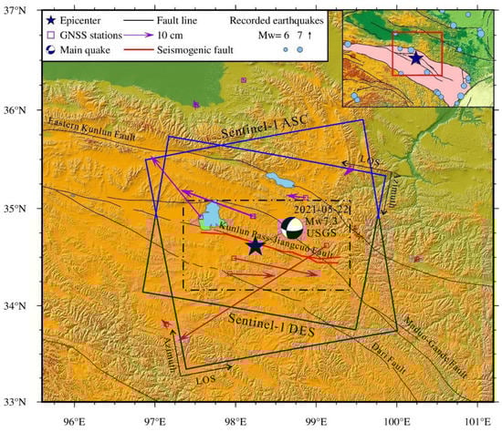
Figure 1.
The record of historic earthquakes around the 2021 Maduo earthquake and the ground coverage of Sentinel-1 data used in this study. The blue star denotes the epicenter of the 2021 Maduo earthquake, black lines denote the known fault lines, blue solid rectangles indicate the ground coverage of the used Sentinel-1 TOPS data, violet arrows represent the coseismic horizontal GNSS deformation caused by the Maduo earthquake (as derived from the work of Li et al. (2021) [27]), red lines represent the surface rupture traces. The coverage of black dashed rectangle is the focused study area.
2.2. Across-Track Displacements Derived from DInSAR and POT Techniques
We used the GAMMA software to process the collected Sentinel-1 acquisitions with the DInSAR, BOI, POT and MAI techniques [28]. In order to ensure high co-registration accuracy of a pair of SAR images, we used a geometrical co-registration method and followed by the enhanced spectral diversity (ESD) to mitigate the residual misregistration [29,30,31,32]. Then we applied a common two-pass DInSAR processing strategy to retrieve the coseismic deformation. The multilook factors were set to 28:7 in range and azimuth directions for improving the signal-to-noise (SNR) and maintaining quality interferometric coherence. The Shuttle Radar Topography Mission (SRTM) digital elevation model with a 30 m resolution (provided by Consortium for Spatial Information (CGIAR-CSI), available at https://srtm.csi.cgiar.org/srtmdata, accessed on 7 June 2021) was employed to model the topographic phase component, and then we removed it from the prior interferograms. After using the Goldstein algorithm [33] to filter noise in the interferograms, the minimum-cost-flow (MCF) method was utilized to unwrap the differential interferograms [34]. Finally, a previously proposed bi-linear algorithm was used to model and mitigate the phase ramps based on the far-field observations with high coherence [4,35]. The coseismic surface displacements derived from the DInSAR method are shown in Figure 2a,b. The azimuth and range patch sizes were set to 256 × 256 pixels and the oversampling factor was set to 2 during POT processing. The range and azimuth offset displacements obtained by the POT approach are shown in Figure 2c,d and Figure 3a,b, respectively.

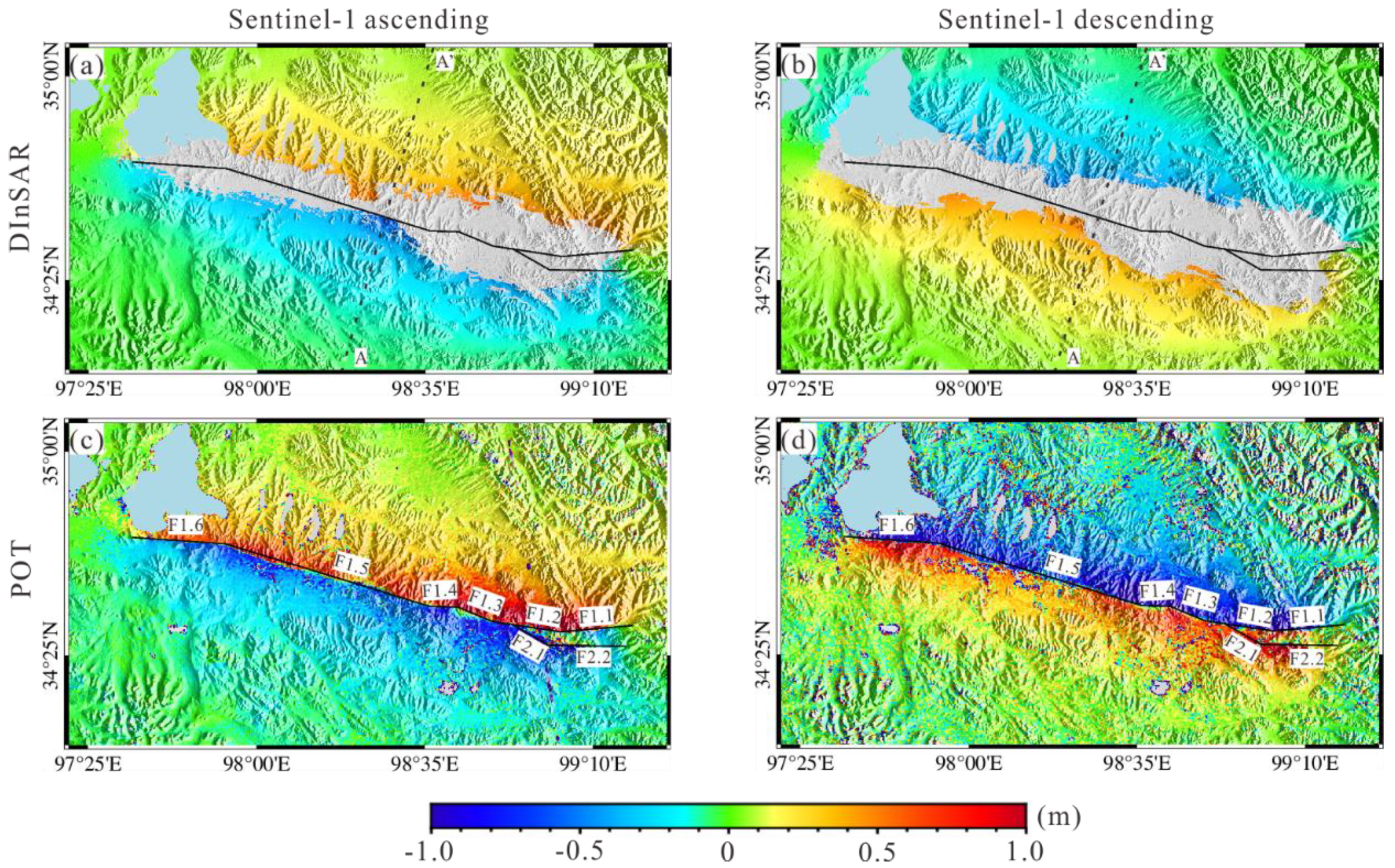
Figure 2.
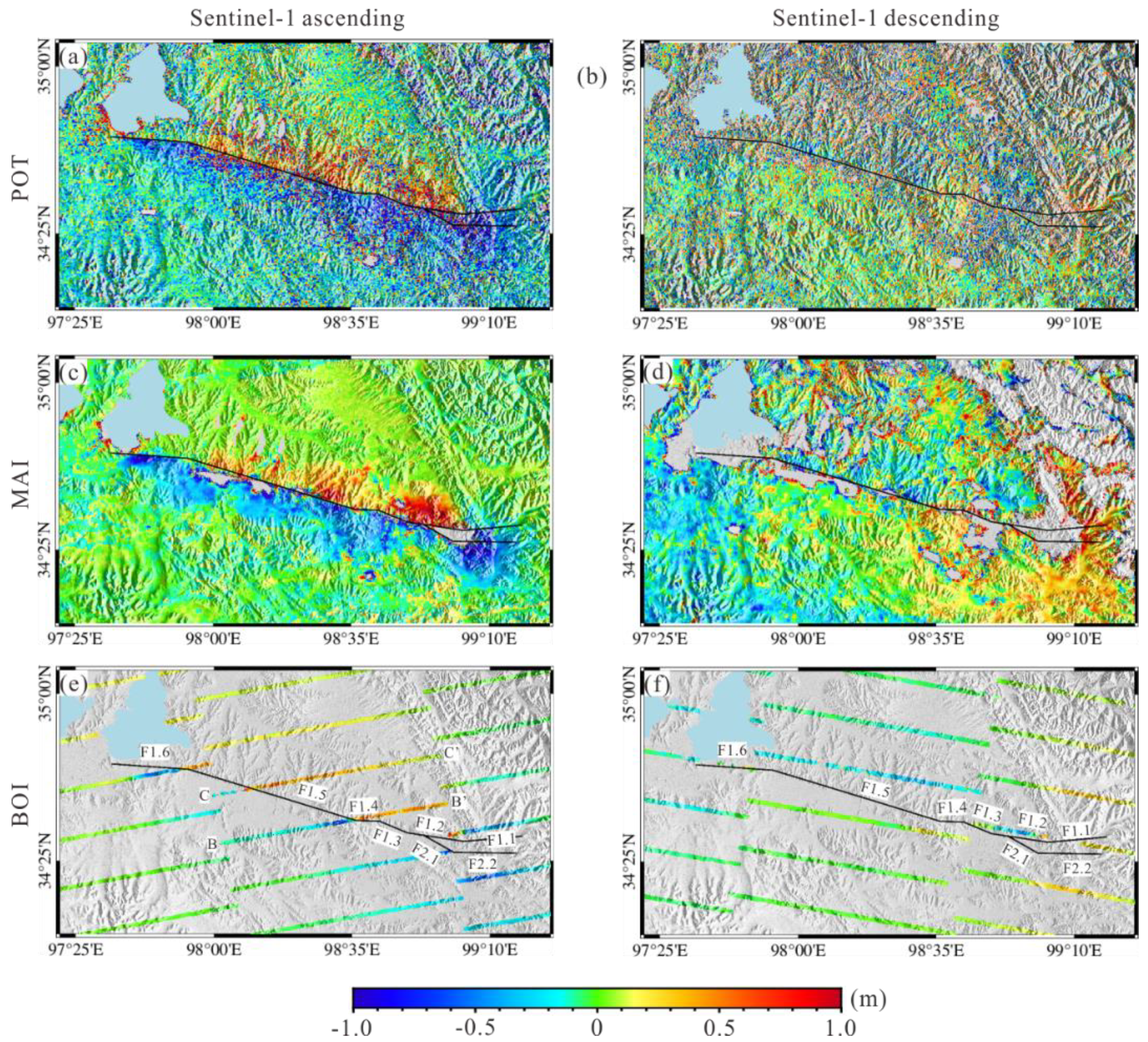
Across-track displacements of the 2021 Maduo earthquake derived from Sentinel-1 TOPS data, utilizing DInSAR for ascending (a) and descending (b) tracks and range offsets derived from ascending (c) and descending (d) tracks. The black solid lines, marked by F1 and F2, indicate the two distinct fault lines extracted with the POT technique. The black dashed line is the AA′ profile, which is used to analyze the across-track displacements in Section 2.4.

Figure 3.
Along-track displacements of the 2021 Maduo earthquake derived from Sentinel-1 TOPS data; we utilized POT method for ascending (a) and descending (b) tracks, azimuth offsets derived from ascending (c) and descending (d) tracks, and BOI for ascending (e) and descending (f) tracks. The black solid lines, marked by F1 and F2, indicated the two distinct fault lines extracted by POT technique. The two black dashed lines indicate the BB′ and CC′ profiles, which are used to analyze the along-track displacements in Section 2.4.
Figure 2 shows that the InSAR data derived from DInSAR measurements were missing in the near-fault zone, likely due to the large displacement gradients, but the coseismic displacement fields mapped with the POT method were nearly complete. We found clear displacement discontinuities between the fault foot wall and the hanging wall in the range offset displacement fields, and it is easy to identify two distinct faults (F1 and F2), marked with solid black lines, in Figure 2. Detailed field investigations conducted by utilizing a Phantom 4 Pro RTK DJI drone revealed that the western segment roughly followed the Jiangcuo fault, and its eastern segment might have been a newborn fault [23]. Our extracted fault lines suggested that the western part of F1 most likely corresponds to part of the Jiangcuo fault, which is consistent with the work of Ren et al. [23]. Additionally, F2 was found to be located on the southern side of the eastern end of fault F1. According to the significant variations of the fault strike, F1 was divided into six segments (see F1.1–F1.6 labeled in Figure 2) and F2 was divided into two segments (see F2.1–F2.2 labeled in Figure 2); the total lengths were 162 km for F1 and ~36 km for F2, respectively. These extracted strike angles and fault segment lengths were used as the initial values for fault geometry parameter inversion.
All the coseismic LOS displacement fields showed antisymmetric distributions with respect to the fault line. For the ascending pair (track 99), the northern wall moved towards the satellite with a maximum deformation of ~1.9 m, while the southern wall moved away from the satellite (Figure 2c). For the descending pair (track 106), the pattern of coseismic deformation was reversed to the ascending track, and the northern wall moved away from the satellite with a maximum deformation of ~1.8 m while the southern wall moved towards the satellite (Figure 2d). The characteristics of the InSAR coseismic deformation suggest that this seismic event was mainly dominated by the sinistral strike-motion of the seismogenic fault.
2.3. Along-Track Displacements Derived from POT, MAI and BOI Techniques
The use of two tracks DInSAR measurements from different viewing geometries alone cannot solve 3D displacements. Therefore, it is necessary to use high-quality along-track displacements to retrieve 3D coseismic displacements of the 2021 Maduo earthquake based on the Sentinel-1 TOPS data. We utilized the above-mentioned techniques to obtain the coseismic displacements in the azimuth direction, respectively. Figure 3a,b shows the azimuth offset displacements derived from the POT method, thus revealing the visible azimuth displacements caused by the Maduo earthquakes in both tracks. However, we found severe speckle noise disturbances in the azimuth offset displacements. It can be seen from Figure 3a that the northern side of the F1 moved towards the along-track direction, while the southern side moves away from the along-track direction. Interestingly, the surface motions around F2 primarily moved away from the along-track direction.
MAI, firstly introduced by Bechor & Zebker (2006), is another approach that can be used to obtain azimuth displacements by relying on the interferometric phase [14]. The critical step of this technique is using split-beam processing to divide full-aperture SLC SAR images into two sub-apertures [15,16]. An interferometric pair contains two SLC images that can generate a total of four sub-apertures SLCs. Those four sub-apertures SLCs are used to produce two interferograms via the standard two-pass DInSAR approach. Then the azimuth displacements can be retrieved by employing double-difference processing for forward- and backward-looking interferograms as follows:
where and denote the forward- and backward-looking reference images, and represent the forward- and backward-looking secondary images.
We set the multilook factors to 28:7 in range and azimuth directions to improve interferometric coherence. Moreover, we applied an adaptive filter to the double-difference interferogram three times with adaptive filter exponents and window sizes, respectively, of 0.2/64, 0.4/32 and 0.6/16, for reducing phase noise and increasing the accuracy of the interferometric phase [33]. Then we employed polynomial models to correct residual flat-earth and topographic phase distortions [36]. Figure 3c shows clear coseismic displacement signals in the ascending track, which indicates that the pattern of azimuth displacements derived from MAI is in line with the POT result (Figure 3a).
In the TOPS mode, each subswath consists of a series of consecutive bursts, these “burst overlap areas” are located between two neighboring bursts to ensure no gap in the final processed images, so pixels in burst overlaps are naturally observed twice in two discrepant squinted views. Therefore, the along-track displacements can be retrieved from double-difference burst overlap interferograms, which benefit from the slight differences in squint angles within those burst overlaps. The principle of the Sentinel-1 TOPS imaging mode can be seen in Figure S1. It should be noted that the residual tropospheric and topographic phases are largely canceled out by the double difference during BOI processing [9]. For the C-band SAR sensor (e.g., Sentinel-1), ionospheric disturbances are generally ignored because they rarely occur in low and middle latitude areas. Therefore, phase differences within burst overlaps can achieve accurate along-track measurements. The phase differences derived from two the two interferograms in the forward and backward views can be formed by:
where Δfovl represents spectral separation and Δtaz is the azimuth time interval.
In order to map the accurate along-track displacements with the BOI technique, we used a geometrical co-registration method to roughly estimate the co-registration parameter, enhanced spectral diversity (ESD) to mitigate the residual misregistration, and the early-multilooking to enhance the coherence in burst overlaps [31]. The remaining steps were the same as those of DInSAR processing; details could be found in Section 2.2. Figure 3e,f shows the along-track displacements derived from the BOI technique based on Sentinel-1 TOPS data. Detailed parameters of two pairs of Sentinel-1 TOPS data can be seen in Tables S1 and S2.
Both ascending and descending interferograms (Figure 3e,f) showed the pure and clearly visible along-track displacement signals, especially the high-quality along-track displacements of descending orbit that was not found in the descending tracks of the MAI and POT results. The azimuth displacement signals in near-fault zones were found to be significant, and we found clear displacement discontinuities between northern and southern wall faults within burst overlaps of the ascending track. The interpretation of azimuth displacement fields derived from the BOI method was basically in accordance with the POT and MAI results. It is interesting to note that the azimuth displacements around the F1.1 and F1.2 exhibit movement both away from and towards the along-track direction movements, which suggested that complex slips occurred on F1.1 and F1.2. Furthermore, the maximum along-track displacements were ~1.0 m for the ascending track and ~0.85 m for the descending track.
2.4. Quality Assessment of the Across- and Along-Track Displacements
Because the accuracies of across- and along-track measurements directly affect the quality of the 3D displacement field, they needed to be appropriately weighed for retrieving the 3D displacements by using the WLS method. To estimate the accuracies of the above InSAR measurements, we first deducted the area including coseismic deformation and then counted the standard deviations and mean values of the displacements within a far-field area; this strategy is proposed by Hu et al. (2012) [36]. The assessments of different InSAR measurements are listed in Table 2, where smaller calculated standard deviations indicate higher displacement accuracies.
Table 2.
The accuracies of the across- and along-track displacements derived from DInSAR, POT, MAI and BOI approaches (unit: cm).
The accuracy of the BOI measurements was 4.3 cm in ascending orbit and 3.6 cm in descending orbit, values that are close to that of the DInSAR technique and significantly better than those of the MAI and POT approaches. In addition, the accuracy of the azimuth displacement via the POT method is the worst of the above-mentioned techniques. We were not surprised by the results because the DInSAR, BOI and MAI methods utilize the interferometric phase but with different Doppler frequency bandwidths, but the POT technique uses amplitude information. Additionally, the azimuth displacement accuracies of descending track of the MAI and POT techniques were not as high as that of the ascending track, which may have been caused by the low SNR and interferometric coherence.
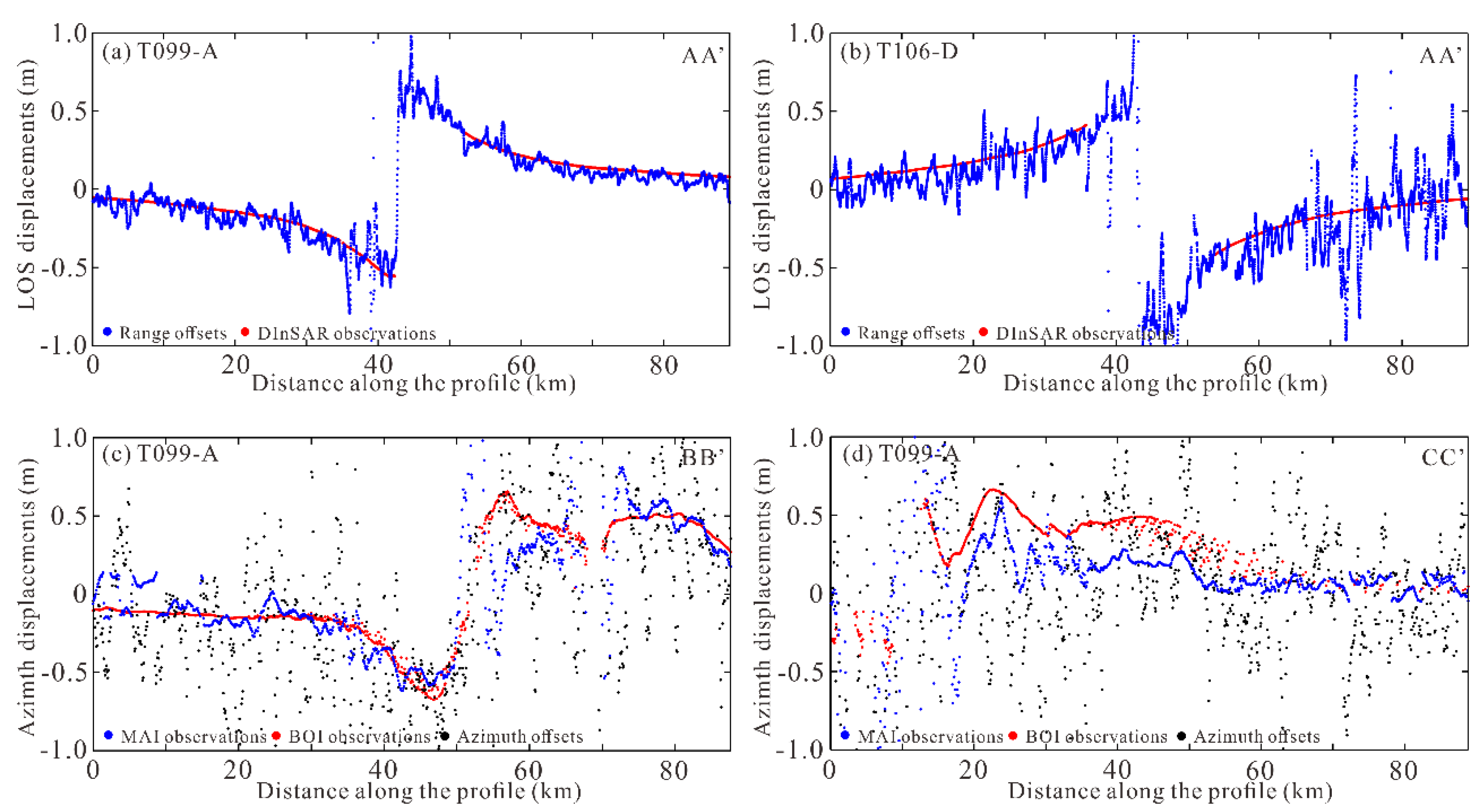
Furthermore, we chose three profiles across the F1 fault to compare the different across- and along-track measurements, as shown in Figure 4a,b. It is clear that the across-track displacements measured with the DInSAR and POT methods were consistent with each other along the AA′ profile, but the range offsets contain more noise. However, the along-track displacements obtained with the MAI, BOI and POT approaches (Figure 4c,d) present significant differences, though the curve trends remained consistent along with the BB′ and CC′ profiles. The along-track displacements from the BOI method were concentrated, but the MAI results were much noisier, and the POT results exhibited oscillations.

Figure 4.
LOS displacements of ascending (a) and descending (b) tracks derived from the DInSAR and POT methods are compared along the AA′ profile. The azimuth displacements of the ascending orbit derived from the MAI, BOI and POT methods are compared along the BB′ (c) and CC′ (d) profiles.
3. Methods
3.1. 3D Displacement Modeling
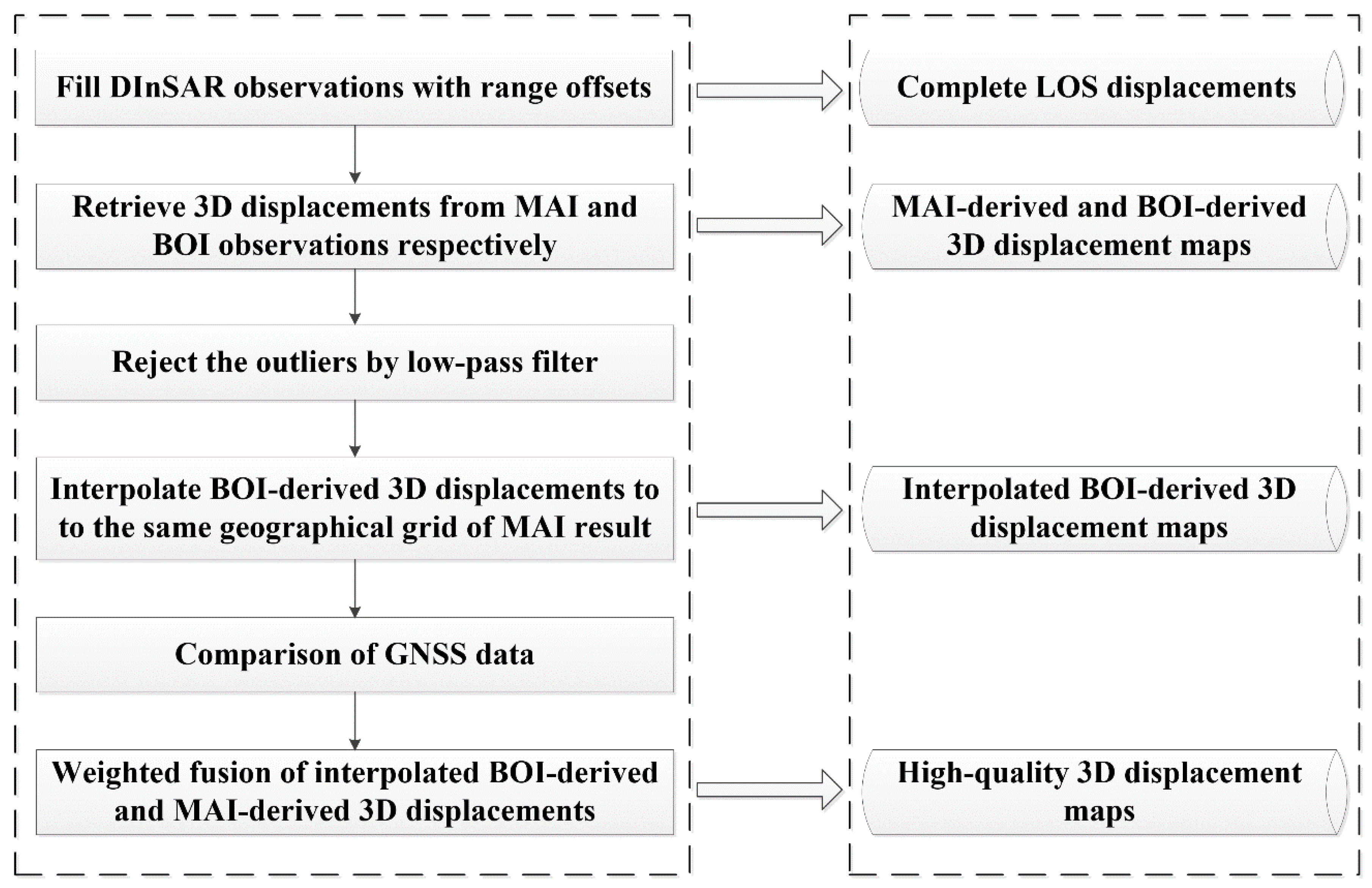
To overcome the disadvantages of the above-mentioned InSAR techniques for retrieving 3D displacement maps from TOPS data, we propose an integrated method to generate high-quality 3D displacements based on the DInSAR, POT, MAI and BOI techniques. The key idea is the comprehensive utilization of the advantages of various InSAR techniques, such as the high precision of DInSAR and BOI measurements, the complete LOS displacement fields that can be obtained by POT technique, and the relatively wider coverage of azimuth displacements that can be derived from the MAI measurements. A flowchart of this integrated method is shown in Figure 5; the crucial step is applying a weighted fusion algorithm to the interpolated BOI-derived and MAI-derived 3D displacements.
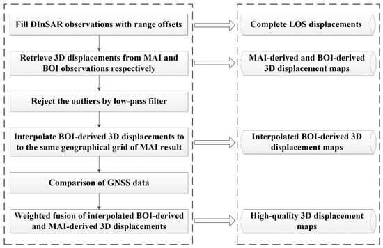
Figure 5.
Flowchart illustrating the process of retrieving high-quality 3D displacement maps based on the integration approach.
Firstly, we filled in the unavailable DInSAR observations of near-field with range offsets derived from the POT technique to obtain complete across-track displacement fields. For an observation target on the ground, across- and along-track displacements could be represented by imaging geometry and 3D surface displacement components as follows [5,7]:
where and are the across- and along-track displacements derived from above-mentioned InSAR measurements, respectively; represents the north–south, east–west and up–down surface deformation components, respectively; is the incidence angle; is the azimuth angle; and denote the noises in the across- and along-track displacements, respectively.
After resampling the across- and along-track displacements to the same geographical location, the MAI-derived and BOI-derived 3D displacements could be solved by combining Equations (3) and (4) through the weighted least square (WLS) method [5,6,7]:
with
where is the weighting matrix, which is the inverse of the covariance matrix of observations, and denote the standard deviations of the across- and along-track displacements, respectively. The standard deviations of each InSAR measurement, which are calculated by the displacements within a far-field area, are listed in Table 2.
Then, the outliers of BOI-derived 3D displacement maps were rejected by a low-pass filter with a cut-off spatial wavelength of 1 km. After that, the BOI-derived 3D displacements were interpolated to the same geographical grid of MAI results (Figure S2). To obtain the weight factors of the InSAR-derived 3D deformation components, the site data (e.g., GNSS and leveling data) were used to calculate the root mean square errors (RMSEs). If there were no situ data, the method proposed by Hu et al. (2014) [5], in which we deducted the area including coseismic deformation and choose a far-field area to calculate the mean values and standard deviations, was adopted. Finally, high-quality 3D displacements were obtained via the simple weighted fusion of the interpolated BOI-derived 3D displacements and MAI-derived 3D displacements :
with
where w denotes the weighting factor, which is calculated by the RMSEs of the InSAR-derived three-dimensional displacements; M and B represent in the MAI and BOI cases, respectively; and are determined via comparisons of GNSS data, as shown in Table 3.
Table 3.
Accuracies of InSAR-derived 3D displacements in comparison to GNSS data (unit: cm).
3.2. Geodetic Modeling
Utilizing the InSAR data for fault slip model inversion involved a highly nonlinear optimization process. It was obvious that the massive data points of observations would result in a severe computing load. Thus, the dense InSAR observations were down-sampled using a quadtree algorithm for enhancing computation efficiency [37]. Before down-sampling, in order to guarantee the quality of the observations, the InSAR observations with interferometric coherence of below 0.6 were abandoned. Finally, 2007 samples of the ascending track and 2230 samples of the descending track were reserved and employed as constraints for determining the fault geometry and slip model.
According to the characteristic of the coseismic InSAR deformation field, F1 was a typically northeast-dipping fault with the left-lateral strike-slip motion. Thus, the extracted strike angles from the POT method for six F1 segments (from southeast to northwest) were set to 264°, 279°, 292°, 269°, 287° and 273°. The extracted strike angles of two F2 segments were 120° and 93°. Based on the USGS solution and field investigations, we set dip and rake angles of 67° and 0°, respectively, as initial values for fault geometry parameter inversion, together with the above-mentioned strike angles.
The along-dip width was set to 30 km for both the F1 and F2 faults. The along-strike lengths of six F1 segments were 23, 22, 12, 9, 68 and 40 km; and the lengths of two F2 segments were set to 13 and 25 km. For the six F1 segments, we set the searching intervals of strike angles to [255°, 275°], [260°, 290°], [285°, 235°], [265°, 275°], [280°, 300°] and [265°, 285°, and those of [110°, 130°] and [85°, 105°] were set for the two F2 segments. All fault segments of F1 and F2 shared the same dip angle interval of [60°, 90°] and rake angle interval of [−40°, 40°]. Furthermore, the top edges of all segments were set to be at the surface based on the interpretation of the field investigations and the coseismic InSAR deformation fields.
We estimated the faulting model of the 2021 Maduo earthquake by using InSAR observations based on the elastic dislocation model [38]. Details of the inversion process detail are discussed in the work of Yang et al. (2019, 2021) [39,40]. Firstly, all the fault planes were discretized into 5 km × 5 km to help us reduce computation costs. Then the simulated annealing algorithm was applied to search for the optimal fault geometry parameters until we obtained a globally minimized misfit between the observed and modeled displacements. To avoid an abrupt variation of slip between adjacent fault patches, the Laplace smoothing constraint was employed in the inversion process. After determining the fault geometry parameters, we discretized the fault planes into a smaller patch with 2 km × 2 km to estimate a more detailed slip distribution.
4. Results
4.1. The 3D Coseismic Displacement Maps of the 2021 Maduo Earthquake
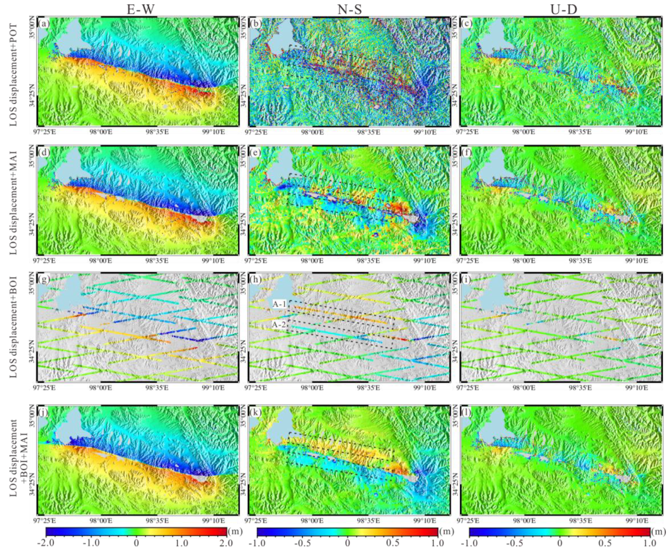
The along-track displacements of descending track were discarded due to the low SNR. We used the above-mentioned datasets to generate 3D displacement maps of the 2021 Maduo earthquake, as shown in Figure 6. The significant east–west (E–W) displacements were distributed along the fault trace, and the north–south (N–S) displacements were relatively small. Additionally, the vertical displacements were concentrated in the near-fault areas, and their magnitudes were the least among the three components. This displacement pattern indicated this seismic event was mainly dominated by the sinistral strike-motion. The displacement pattern of F2 was complex because E–W displacements were significant in the southern side of F2 but slight between the northern side of F2 and the southern side of F1.1–F1.2. Interestingly, all the movements around F2 were directed towards the south in the N–S displacement field. Furthermore, the 3D displacements obtained with the MAI method are decorrelation in the near-fault regions, while those obtained with the POT method are more complete but contain more noise.

Figure 6.
The 3D coseismic displacement maps of the 2021 Maduo earthquake. (a–c) are obtained by integrating complete LOS displacements and POT measurements. (d–f) are obtained by integrating complete LOS displacements and MAI measurements. (g–i) are obtained by integrating complete LOS displacements and BOI measurements. (j–l) are obtained by MAI-derived and interpolated BOI-derived 3D displacements. The color bars are set on the same scale for each displacement component for easier comparison. To enable the comparison of N–S component details, the two black rectangles located in northern and southern walls of the fault are marked “A-1” and “A-2”, respectively.
The high-quality 3D displacement maps derived from BOI measurements (Figure 6g–i) helped reveal detailed surface movements, especially for the north–south component. However, each burst overlap area only covered ~1.5 km in the azimuth direction, which was occupied about 10% of each burst length. The burst overlap area marked "A-1" in Figure 6h, in which the BOI results showed clear northward surface movements, was located on the northern side of F1. However, the POT and MAI results indicated that the north-south displacements of “A-1” were not clear and significant. The maximum horizontal displacements of the BOI result were ~2.3 m of westward movement and ~1.0 m of downward movement, which were located around the eastern end of F1. Figure 6j–l shows the high-quality 3D displacement maps derived from the weighted fusion of MAI and BOI results, and it was clear that the north–south displacement field was cleaner and more continuous than that of the MAI and POT results alone. The north–south displacement pattern of “A-2” was consistent with the MAI results, but that of “A-1” obviously contained more northward movements. A comparison of the 3D coseismic displacement fields obtained with different strategies indicated that the 3D coseismic displacements derived from our proposed method retained not only the high-precision of the BOI measurements but also the wide coverage of the MAI measurements.
In order to quantitatively assess the 3D displacement fields derived from different datasets, the coseismic GNSS displacements (see Figure 1) were used to assess the qualities of those 3D displacements; details regarding GNSS data can be seen in the work of Li et al. (2021) [27]. The RMSEs between GNSS data and the aforementioned InSAR-derived 3D displacements were calculated, as shown in Table 3. The RMSEs of the north–south component were the largest of three displacement components, with 21.3, 13.6, 6.3 and 5.5 cm for the POT, MAI, the weighted fusion case and BOI results, respectively. The accuracies of the north-south component agreed well with the corresponding accuracies of the different azimuth measurement techniques. The RMSEs of the 3D displacement fields derived from the weighted fusion method were 5.8, 6.3 and 1.7 cm in east–west, north–south and up–down directions, respectively, suggesting that our proposed method can retrieve high-quality 3D displacement. Furthermore, because the vertical displacements caused by the 2021 Maduo earthquake were small, the vertical component accuracies of the four results were similar.
4.2. Fault Geometry and Slip Model
After finishing the steps of Section 3.2, the fault geometry parameters were determined, as shown in Table 4. The best-fitting strike angles were 263.9° for F1.1, 280.5° for F1.2, 287.2° for F1.3, 271.3° for F1.4, 288.0° for F1.5 and 275.0° for F1.6. The estimated fault geometry indicated a north-dipping fault of F1 with an average best-fitting strike angle of 277.6°, which was different from the USGS solution of 92° but in agreement with the GCMT solution of 282°. The estimated average dip angle of F1 was 79.5°, which was between the USGS solution of 67° and the GCMT solution of 83°. F2 was a south-dipping fault with strike angles of 126.4° and 93.2° for its two segments, and its average dip angle was 77.85°.
Table 4.
Fault parameters of the 2021 Maduo earthquake solved by DInSAR observations.
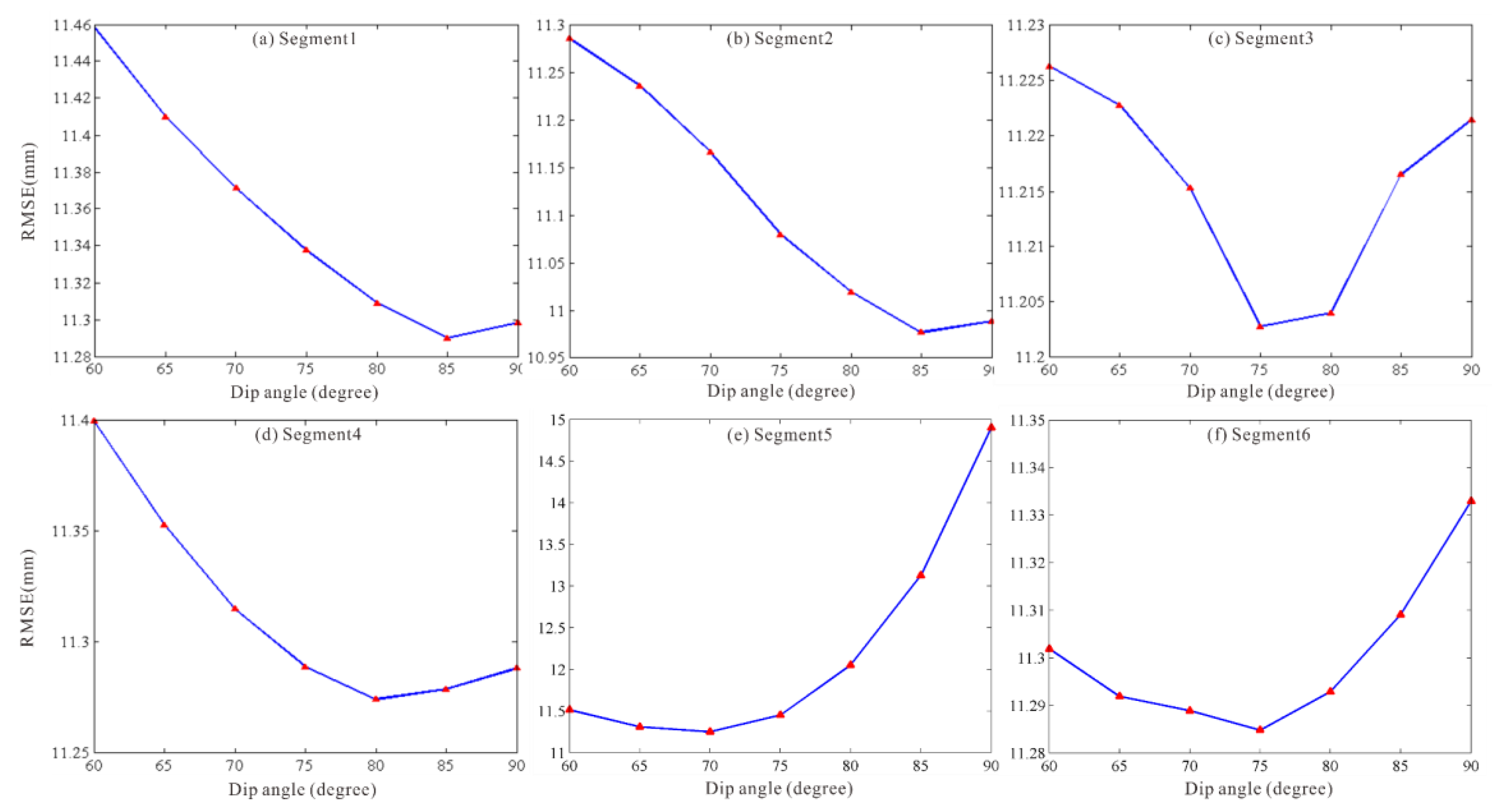
In addition, we repeated the searching process one hundred times with random initial values and random subsets of 95% of the down-sampled InSAR data to estimate the 1-sigma standard derivation of each parameter estimate, as shown in Table 4. The estimated uncertainties of the slip distributions were based on the inferred fault geometry model, as shown in Figure 7. The trade-off curves between the model RMSEs and dip angles for the six segments of F1 are shown in Figure 8. The model misfits were 1.0 and 1.1 cm for the Sentinel-1 ascending and descending DInSAR observations, respectively. The slip model could explain 99.7% and 99.7% of the Sentinel-1 ascending and descending DInSAR observations, respectively, which indicated consistency between the observed and predicted data. The modeled displacements of the ascending and descending DInSAR observations and the surface projection of constructed faults can be seen in Figure S3.

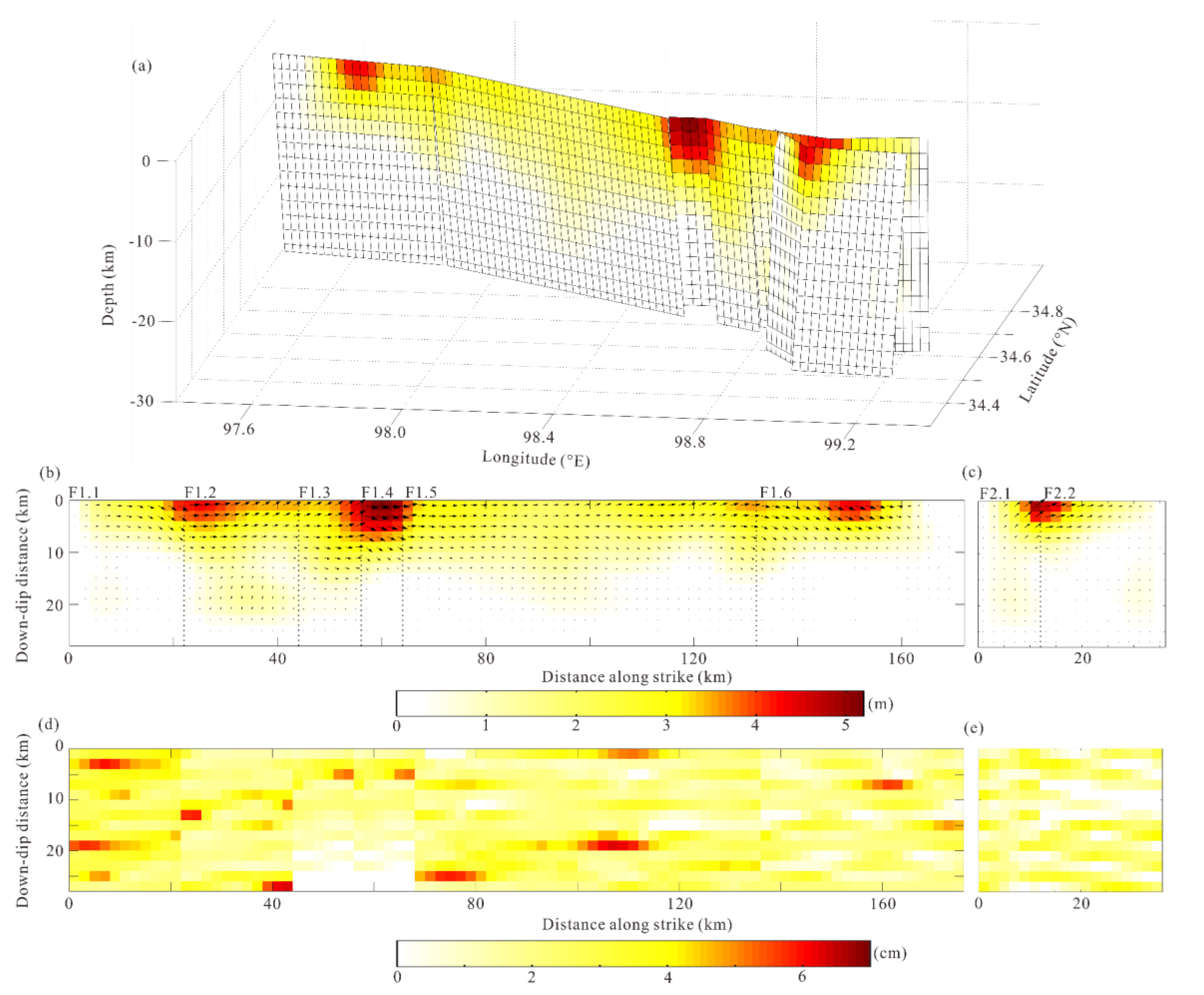
Figure 7.
Fault slip model of the 2021 Maduo earthquake constrained by DInSAR observations. (a) F1 and F2 faulting model with three-dimensional view. Slip distribution on F1 (b) and F2 (c) and the corresponding error distributions on the F1 (d) and F2 (e) fault planes.

Figure 8.
The trade-off curves between the model RMSEs and dip angles for the six segments of F1.
Figure 7 shows the fault slip of the 2021 Maduo earthquake constrained by DInSAR observations, it can be observed that the ruptures of both F1 and F2 were mainly predominated by the sinistral strike-slip motion. In agreement with the field investigations, both of the faults ruptured to the surface. The maximum slip occurred on F1.4 with a magnitude of ~5.1 m. Three slip asperities could be easily distinguished on F1; all of them were located at depths of 0–10 km. Additionally, there was a clear slip asperity on F2 that was concentrated at depths of 0–8 km and distances of 6–20 km along the strike direction, with a peak slip of ~5.2 m. Moreover, the slip on F1.5 was a nearly pure left-strike slip at depths of 0–10 km and at distances of 64–134 km along the strike direction, this slip pattern of F1.5 results in the modeled displacements toward the south direction at the northern side of F1.5 being slightly small, more details were discussed in next section. Furthermore, the seismic moment derived from inferred faulting model was found to be 1.69 × 10²⁰ Nm, equivalent to a moment magnitude of Mw 7.42. The moment magnitude of the inferred source model was slightly larger than that of the USGS and GCMT solutions because the InSAR data contained more post-seismic deformation information due to the long 6/12-day revisit time of the SAR satellite.
4.3. Coulomb Failure Stress Change
Previous investigations have revealed that strong earthquakes, such as the Maduo earthquake partially release long-term accumulated stress and strain, and they routinely follow a fast stress modulation process that is directly related to the faulting of this earthquake [41,42]. Around the seismogenic fault of the Maduo earthquake, there were three major faults: the eastern Kunlun fault, the Maduo–Gande fault and the Dari fault (Figure 1). In order to investigate the effects of the Maduo earthquake on the adjacent major faults, we calculated the static CFS changes on the three above-mentioned fault planes. We set the dip and rake angles of the eastern Kunlun fault and the Maduo–Gande fault to 80° and 0°, respectively. Additionally, the dip and rake angles of the Dari fault were set to 60° and 60°, respectively. The locations and strike angles of the three faults are obtained from the database of Styron and Marco (2020) [43]; the detailed parameters of the adjacent major faults are presented in Table S3.
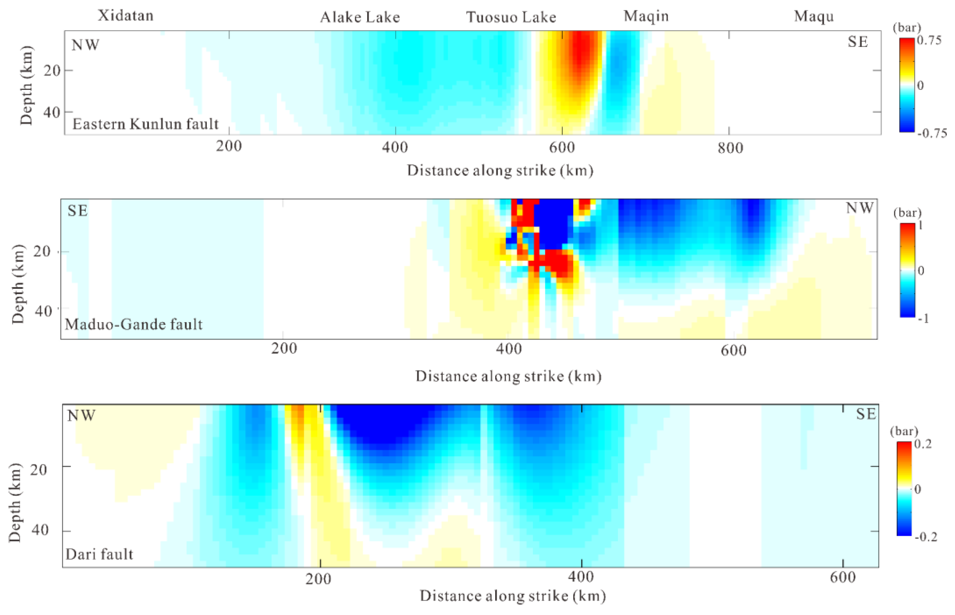
Figure 9 shows the static CFS change on the Alake Lake–Maqin region was significant, but there was little stress change on the northwest of the Xidatan–Alake Lake region and the southeast of the Maqin–Maqu region. A region of clearly significant stress increase could be seen in the Tuosuo Lake–Maqin segment, with a maximum of 0.75 bar and an average of 0.21 bar. There was little effect on the southeastern segment of the Maduo–Gande fault (Figure 9) since the calculated CFS change was approximate zero. However, on the northwestern segment of the Maduo–Gande fault, a negative CFS change zone with an average of 0.52 bar was found to be located at depths of 0–20 km and distances of 500–650 km from the southeastern fault plane. For the Dari fault (Figure 9), the faulting of the Maduo earthquake appeared to cause little effect on the whole fault plane. Consequently, we infer that the Tuosuo Lake–Maqu segment of the Eastern Kunlun fault could be a zone at high risk of future earthquake rupture.

Figure 9.
Static Coulomb failure stress (CFS) change caused by the Maduo earthquake on the three major faults.
5. Discussion
5.1. Fault Slip Model Estimated by the Joint Utilization of DInSAR and BOI
To investigate the advantage of high accuracy azimuth displacement measurements for slip model inversion, we estimated the slip model of the 2021 Maduo earthquake jointly constrained by DInSAR and BOI observations using the same method and initial values mentioned in Section 3.2. The best-fitting fault geometry parameters and the corresponding uncertainties are shown in Table 5. The estimated strike angles were 262.0° for F1.1, 278.3° for F1.2, 289.8° for F1.3, 272.8° for F1.4, 286.3° for F1.5 and 277.1° for F1.6 The average dip and rake angles of F1 were 79.3° and 5.8°, respectively. The fault geometry parameters of F1 determined with the two different datasets were similar. The strike angles of two F2 segments were separately 124.8° and 92.3°, which was basically consistent with the inversion result of DInSAR observations. The model misfits were 1.2 and 1.3 cm for ascending and descending DInSAR observations, respectively, and 3.0 and 3.9 cm for ascending and descending BOI observations respectively. For ascending and descending tracks, the slip model could explain 99.6%, 99.6%, 94.9% and 80% of the DInSAR and BOI observations, respectively. The modeled displacements and residuals of the ascending and descending DInSAR and BOI observations can be seen in Figure S4.
Table 5.
Fault parameters of the 2021 Maduo earthquake solved by DInSAR and BOI observations.
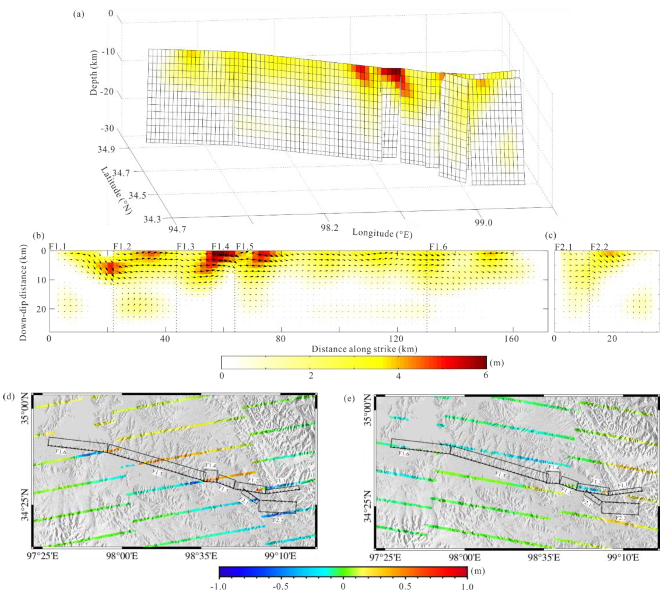
In Figure 10d,e, one could be observed some burst overlap areas across the fault lines, especially the BOI observations of the ascending track. However, the DInSAR observations (Figure 2a,b) were missing in the near-fault zone, likely due to the interferometric decorrelation. Thus, the inferred slip model constrained by the high-quality azimuth displacements showed that a more detailed and complex slip distribution occurred on F1. There were three slip asperities that could be easily distinguished on F1. The faulting pattern of F1.2 was predominated by the sinistral strike-slip motion and with some thrusting at depths of 0–8 km, and then it progressively transformed into a mixed-mode of left-lateral strike-slip and normal dip-slip motion on F1.3. The slip pattern of F1.5 was a mixed mode of left-lateral strike-slip and dip-slip motion. The slip pattern of the F2 fault entirely comprised left-lateral strike-slip motion on F2.1, and then it transformed into a mixed mode of left-lateral strike-slip and normal dip-slip motion on F2.2. The maximum slip occurred on F1.4 with a magnitude of ~6.0 m. The faulting motion on the F1 and F2 segments released 87.5% and 12.5% of the whole seismic moment, respectively. Furthermore, the total geodetic moment estimated from our inferred faulting model was 1.75 × 10²⁰ Nm, equivalent to a moment magnitude of Mw 7.44.

Figure 10.
Fault slip model of the 2021 Maduo earthquake constrained by DInSAR and BOI observations: (a) F1 and F2 faulting model with three-dimensional view; slip distribution on F1 (b) and F2 (c) with planar view; inferred fault models projected onto the ascending (d) and descending (e) azimuth displacement fields derived from the BOI technique. Black rectangles indicate the surface projection of the constructed faults.
5.2. Synthetic 3D Displacement Maps
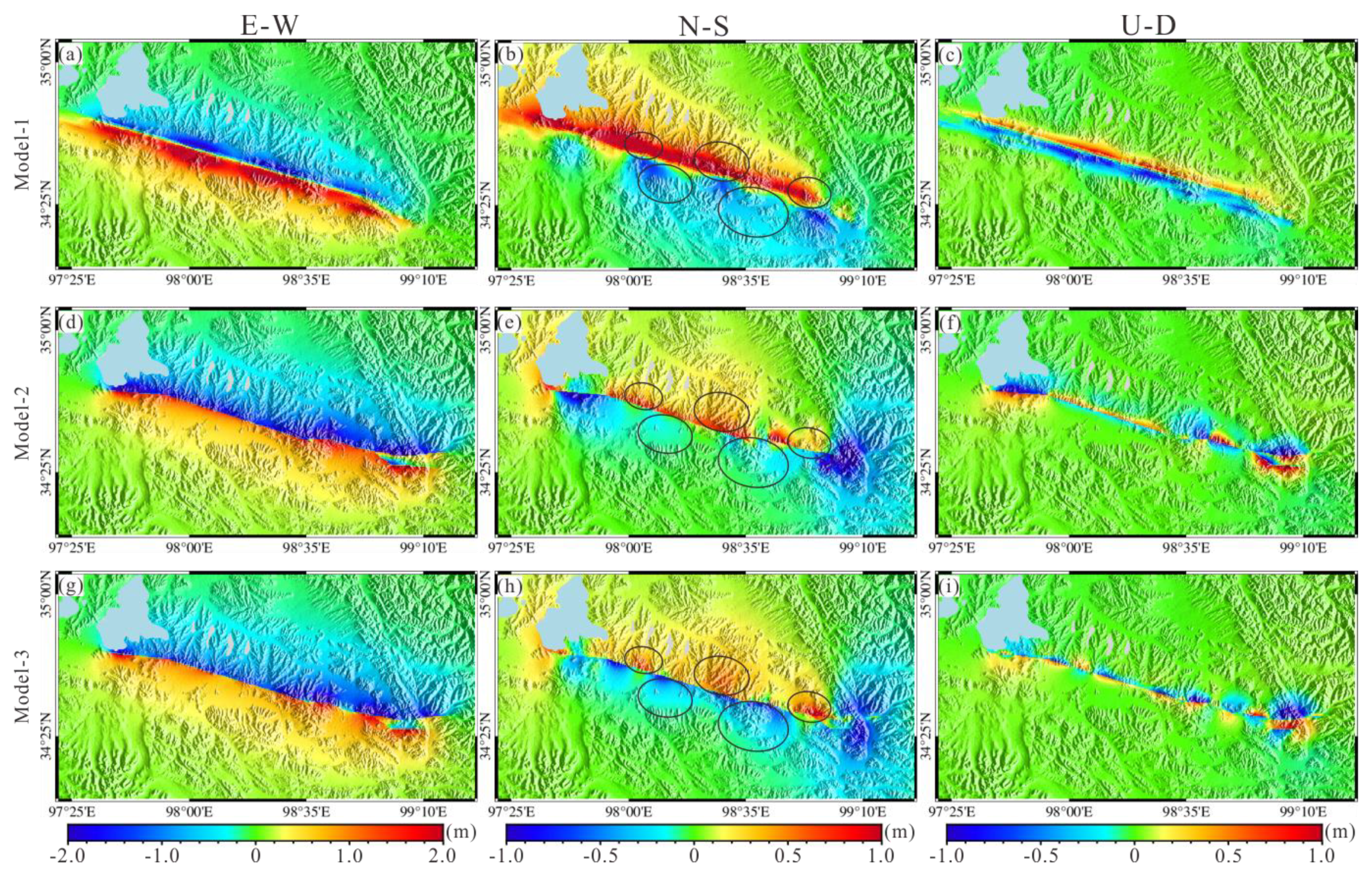
To further analyze the retrieved 3D coseismic displacement fields from the across- and along-track measurements of Sentinel-1 TOPS data, synthetic 3D coseismic displacements were calculated from the three slip models constrained by different datasets. The first slip model of the 2021 Maduo earthquake was available from USGS (it is available at (https://earthquake.usgs.gov/earthquakes/eventpage/us7000e54r/finite-fault, accessed on 7 June 2021). Figure 11a–c shows the synthetic 3D displacements derived from the slip model of USGS (named Model-1), we could find that the overall deformation pattern was in agreement with the observed 3D displacement fields, though the magnitude and detailed spatial distribution were clearly different. The discrepancies may have resulted from the use of teleseismic data with low spatial resolution, which does not have robust constraints for the fault geometry inversion.
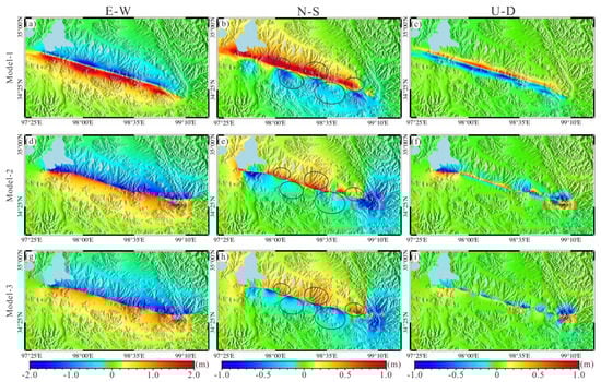
Figure 11.
Synthetic 3D coseismic displacement maps from the source models are constrained by different datasets. Model–1 was modeled from the slip model of USGS (a–c), Model–2 was modeled from the slip model only constrained by DInSAR observations (d–f), Model–3 was modeled from the slip model jointly constrained by DInSAR and BOI observations (g–i). The three panels from left to right indicate the east–west, north–south and up–down displacement components, respectively.
In contrast to teleseismic data, the use of InSAR measurement allowed us to provide a detailed map of crustal deformation with high spatial resolution. We obtained the synthetic 3D displacement map from the slip model (Figure 7b) only constrained by DInSAR observations (Model-2), as shown in Figure 11d–f. These synthetic 3D displacements were basically consistent with observed results, especially the E–W displacements, but there were still some discrepancies in the N–S displacement field. It could be seen from Figure 11e that surface movements around the southern side of the fault (as marked in black ellipses) were underestimated, though the results were obviously better than those of Model-1. Model-3 was jointly constrained by DInSAR and BOI observations, as shown in Figure 11g–i. The E–W and N–S displacement components were both modeled well and very similar to the observed results. The N–S displacements of Model-3 in the southern side of the fault clearly contained more details, and the deformation pattern of those black ellipse areas (Figure 11h) was consistent with the observed N–S displacements. The differences between Model-2 and Model-3 were due to the fact that the slip model includes more normal dip-slip motion on the F1.5 (Figure 10b). An analysis of the 3D synthetic displacement maps of the three models indicated that source model inversion was necessary to introduce the high-quality BOI observations as constraints, and it will be helpful to understand the characteristics of the focal mechanisms to obtain more detailed slip distributions.
6. Conclusions
In this study, we propose an integrated approach for mapping three-dimensional coseismic displacement fields by utilizing the DInSAR, POT, MAI and BOI techniques. In a case study of the 2021 Maduo earthquake, ascending and descending Sentinel-1 TOP data were employed to map the across and along-track coseismic displacements. We used the DInSAR and POT techniques to obtain the across-track displacements and utilized the POT, MAI and BOI methods to obtain along-track displacements. Then, we quantitatively assessed different displacements by calculating the standard deviations of the far-field areas. The accuracies of DInSAR and BOI measurements were similar, both of them between 2.8 and 4.3 cm. The RMSEs between the GNSS data and the high-quality 3D displacement fields are 5.8, 6.3 and 1.7 cm in east–west, north–south and up–down directions, respectively. Furthermore, two coseismic faulting models were separately estimated with just DInSAR data and a combination of DInSAR and BOI observations, both of which suggested that this seismic event was predominated by left-lateral strike-slip motion mixed with some dip-slip movements. The total geodetic moment estimated from the faulting model constrained by the DInSAR and BOI observations was 1.75 × 10²⁰ Nm, corresponding to a Mw 7.44 event. A comparison of the two slip models indicated that finer slip distribution could be estimated by introducing high-quality BOI measurements of near-fault areas. The calculated static CFS indicated that the Tuosuo Lake–Maqu segment of the Eastern Kunlun fault could be a zone at high risk of future earthquake rupture.
Supplementary Materials
The following are available online at https://www.mdpi.com/article/10.3390/rs13234847/s1, Figure S1. Principle of Sentinel-1 TOPS imaging mode; Figure S2. The interpolated BOI-derived 3-D displacement fields of the 2021 Maduo earthquake; Figure S3. Modeled DInSAR displacements based on the faulting model constrained by only DInSAR observations; Figure S4. Modeled DInSAR and BOI displacements based on the faulting model jointly estimated by DInSAR and BOI measure-ments; Table S1. Parameters of ascending Sentinel-1TOPS data used in this study (track 99); Table S2. Parameters of descending Sentinel-1TOPS data used in this study (track 106); Table S3. Parameters for the adjacent major faults’ Table S4 Root-mean-square errors (RMSEs) of each model.
Author Contributions
Conceptualization, L.X.; methodology and software, L.X. and Y.-H.Y.; validation, Q.X. and J.-J.Z.; resources, Y.-H.Y. and Q.C.; writing–original draft preparation, L.X.; writing–review and editing, X.-W.L. and L.X.; visualization, Q.X. and J.-J.Z.; supervision, Q.C.; funding acquisition, Q.C. and Y.-H.Y. All authors have read and agreed to the published version of the manuscript.
Funding
This work is supported by the National Key Research and Development Program of China (Grant No. 2017YFB0502700), the Fund for Creative Research Groups of China (41521002), the Applied Basic Research Program of Science & Technology Department of Sichuan Province (2020YJ0116) and the Open Funding Project of State Key Laboratory of Geohazard Prevention and Geoenvironment Protection (SKLGP2020K019).
Data Availability Statement
The generated datasets including those of the ascending and descending coseismic across- and along-track displacement fields, and the InSAR-derived faulting model are available from the corresponding author on reasonable request. The original Sentinel images can be acquired from the website of the ESA (European Space Agency).
Acknowledgments
We appreciate the encouraging and constructive suggestions from editors and reviewers for significantly improving the manuscript. The Sentinel-1 SAR images were provided by the ESA (European Space Agency). Most of the figures were plotted with the Generic Mapping Tool (GMT) software provided by Wessel and Smith (1998).
Conflicts of Interest
The authors declare no conflict of interest.
References
- Biggs, J.; Wright, T.J. How satellite InSAR has grown from opportunistic science to routine monitoring over the last decade. Nat. Commun. 2020, 11, 3863. [Google Scholar] [CrossRef] [PubMed]
- Bischoff, C.A.; Ferretti, A.; Novali, F.; Uttini, A.; Giannico, C.; Meloni, F. Nationwide deformation monitoring with SqueeSAR using Sentinel-1 data. Proc. Int. Assoc. Hydrol. Sci. 2020, 382, 31–37. [Google Scholar] [CrossRef] [Green Version]
- Morishita, Y.; Lazecky, M.; Wright, T.J.; Weiss, J.R.; Elliott, J.R.; Hooper, A. LiCSBAS: An open-source InSAR time series analysis package integrated with the LiCSAR automated Sentinel-1 InSAR processor. Remote. Sens. 2020, 12, 424. [Google Scholar] [CrossRef] [Green Version]
- Wright, T.J.; Parsons, B.E.; Lu, Z. Toward mapping surface deformation in three dimensions using InSAR. Geophys. Res. Lett. 2004, 31, L01607. [Google Scholar] [CrossRef] [Green Version]
- Hu, J.; Li, Z.W.; Ding, X.L.; Zhu, J.J.; Zhang, L.; Sun, Q. Resolving three-dimensional surface displacements from InSAR measurements: A review. Earth-Sci. Rev. 2014, 133, 1–17. [Google Scholar] [CrossRef]
- He, P.; Wen, Y.; Xu, C.; Chen, Y. High-quality three-dimensional displacement fields from new-generation SAR imagery: Application to the 2017 Ezgeleh, Iran, earthquake. J. Geod. 2019, 93, 573–591. [Google Scholar] [CrossRef]
- Fialko, Y.; Simons, M.; Agnew, D. The complete (3-D) surface displacement field in the epicentral area of the 1999 Mw7. 1 Hector Mine earthquake, California, from space geodetic observations. Geophys. Res. Lett. 2001, 28, 3063–3066. [Google Scholar] [CrossRef] [Green Version]
- Wang, X.; Liu, G.; Yu, B.; Dai, K.; Zhang, R.; Ma, D.; Li, Z. An integrated method based on DInSAR, MAI and displacement gradient tensor for mapping the 3D coseismic deformation field related to the 2011 Tarlay earthquake (Myanmar). Remote. Sens. Environ. 2015, 170, 388–404. [Google Scholar] [CrossRef]
- Grandin, R.; Klein, E.; Métois, M.; Vigny, C. Three-dimensional displacement field of the 2015 Mw8. 3 Illapel earthquake (Chile) from across-and along-track Sentinel-1 TOPS interferometry. Geophys. Res. Lett. 2016, 43, 2552–2561. [Google Scholar] [CrossRef] [Green Version]
- Michel, R.; Avouac, J.P.; Taboury, J. Measuring near field coseismic displacements from SAR images: Application to the Landers earthquake. Geophys. Res. Lett. 1999, 26, 3017–3020. [Google Scholar] [CrossRef] [Green Version]
- Jiang, H.; Feng, G.; Wang, T.; Bürgmann, R. Toward full exploitation of coherent and incoherent information in Sentinel-1 TOPS data for retrieving surface displacement: Application to the 2016 Kumamoto (Japan) earthquake. Geophys. Res. Lett. 2017, 44, 1758–1767. [Google Scholar] [CrossRef] [Green Version]
- Casu, F.; Manconi, A.; Pepe, A.; Lanari, R. Deformation time-series generation in areas characterized by large displacement dynamics: The SAR amplitude pixel-offset SBAS technique. IEEE Trans. Geosci. Remote. Sens. 2011, 49, 2752–2763. [Google Scholar] [CrossRef]
- Chen, Q.; Luo, R.; Yang, Y.H.; Yong, Q. Method and Accuracy of Ex tracting Surface Deformation Field from SAR Image Coregistration. Acta Geod. Cartogr. Sin. 2015, 44, 301–308. (In Chinese) [Google Scholar] [CrossRef]
- Bechor, N.B.; Zebker, H.A. Measuring two-dimensional movements using a single InSAR pair. Geophys. Res. Lett. 2006, 33, L16311. [Google Scholar] [CrossRef] [Green Version]
- Jung, H.S.; Won, J.S.; Kim, S.W. An improvement of the performance of multiple-aperture SAR interferometry (MAI). IEEE Trans. Geosci. Remote. Sens. 2009, 47, 2859–2869. [Google Scholar] [CrossRef]
- Jung, H.S.; Lu, Z.; Zhang, L. Feasibility of along-track displacement measurement from Sentinel-1 interferometric wide-swath mode. IEEE Trans. Geosci. Remote. Sens. 2012, 51, 573–578. [Google Scholar] [CrossRef]
- De Zan, F.; Guarnieri, A.M. TOPSAR: Terrain observation by progressive scans. IEEE Trans. Geosci. Remote. Sens. 2006, 44, 2352–2360. [Google Scholar] [CrossRef]
- Liu, J.; Hu, J.; Li, Z.; Ma, Z.; Wu, L.; Jiang, W.; Zhu, J. Complete three-dimensional coseismic displacements related to the 2021 Maduo earthquake in Qinghai Province, China from Sentinel-1 and ALOS-2 SAR images. Sci. Bull. 2021. [Google Scholar] [CrossRef]
- Hooper, A. Large-scale, high-resolution maps of interseismic strain accumulation from Sentinel-1, and incorporation of along-track measurements. In Proceedings of the EGU General Assembly 2021, online, 19–30 April 2021. [Google Scholar] [CrossRef]
- Li, X.; Jónsson, S.; Cao, Y. Interseismic Deformation from Sentinel-1 Burst-Overlap Interferometry: Application to the Southern Dead Sea Fault. Geophys. Res. Lett. 2021, 48, e2021GL093481. [Google Scholar] [CrossRef]
- Li, P.; Liao, L.; Feng, J.; Liu, P. Numerical simulation of relationship between stress evolution and strong earthquakes around the Bayan Har block since 1900. Chin. J. Geophys. 2019, 62, 4170–4188. (In Chinese) [Google Scholar] [CrossRef]
- Pan, J.; Bai, M.; Li, C.; Liu, F.; Li, H.; Liu, D.; Li, C. Coseismic surface rupture and seismogenic structure of the 2021-05-22 Maduo (Qinghai) MS 7.4 earthquake. Acta Geol. Sin. 2021, 95, 1655–1670. [Google Scholar]
- Ren, J.; Zhang, Z.; Gai, H.; Kang, W. Typical Riedel shear structures of the coseismic surface rupture zone produced by the 2021 Mw 7.3 Maduo earthquake, Qinghai, China, and the implications for seismic hazards in the block interior. Nat. Hazards Res. 2021. [Google Scholar] [CrossRef]
- Zhan, Y.; Liang, M.; Sun, X.; Huang, F.; Zhao, L.; Gong, Y. Deep structure and seismogenic pattern of the 2021.5.22 Madoi (Qinghai) Ms7.4 earthquake. Chin. J. Geophys. 2021, 64, 2232–2252. (In Chinese) [Google Scholar] [CrossRef]
- Wang, W.; Fang, L.; Wu, J.; Tu, H.; Chen, L.; Lai, G. Aftershock sequence relocation of the 2021 MS7.4 Maduo Earthquake, Qinghai, China. Sci. China Earth Sci. 2021, 64, 1371–1380. [Google Scholar] [CrossRef]
- U.S. Geological Survey (USGS). M7.3-Southern Qinghai, China. 2021. Available online: https://earthquake.usgs.gov/earthquakes/eventpage/us7000e54r/executive (accessed on 7 June 2021).
- Li, Z.C.; Ding, K.H.; Zhang, P.; Wen, Y.; Zhao, L.; Chen, J. Co-seismic deformation and slip distribution of 2021 M W 7.4 Madoiearthquake from GNSS observation. Geomat. Inf. Sci. Wuhan Univ. 2021, 46, 1489–1497. [Google Scholar] [CrossRef]
- Wegmüller, U.; Werner, C. Gamma SAR Processor and Interferometry Software; ESA SP (Print); ESA Publications Division: Noordwijk, The Netherlands, 1997; pp. 1687–1692. [Google Scholar]
- Scheiber, R.; Moreira, A. Coregistration of interferometric SAR images using spectral diversity. IEEE Trans. Geosci. Remote. Sens. 2000, 38, 2179–2191. [Google Scholar] [CrossRef]
- Liu, G.X.; Ding, X.L.; Li, Z.L.; Chen, Y.Q.; Zhang, G.B. Co-registration of satellite SAR complex images. Acta Geod. Cartogr. Sin. 2001, 30, 60–66. [Google Scholar]
- Prats-Iraola, P.; Scheiber, R.; Marotti, L.; Wollstadt, S.; Reigber, A. TOPS interferometry with TerraSAR-X. IEEE Trans. Geosci. Remote. Sens. 2012, 50, 3179–3188. [Google Scholar] [CrossRef] [Green Version]
- Ma, Z.F.; Jiang, M.; Huang, T. A sequential approach for Sentinel-1 TOPS time-series co-registration over low coherence scenarios. IEEE Trans. Geosci. Remote. Sens. 2020, 59, 4818–4826. [Google Scholar] [CrossRef]
- Goldstein, R.M.; Werner, C.L. Radar interferogram filtering for geophysical applications. Geophys. Res. Lett. 1998, 25, 4035–4038. [Google Scholar] [CrossRef] [Green Version]
- Chen, C.W.; Zebker, H.A. Network approaches to two-dimensional phase unwrapping: Intractability and two new algorithms. JOSA A 2000, 17, 401–414. [Google Scholar] [CrossRef]
- Simons, M.; Fialko, Y.; Rivera, L. Coseismic deformation from the 1999 M w 7.1 Hector Mine, California, earthquake as inferred from InSAR and GPS observations. Bulletin of the Seismological. Soc. Am. 2002, 92, 1390–1402. [Google Scholar] [CrossRef]
- Hu, J.; Li, Z.W.; Ding, X.L.; Zhu, J.J.; Zhang, L.; Sun, Q. 3D coseismic displacement of 2010 Darfield, New Zealand earthquake estimated from multi-aperture InSAR and D-InSAR measurements. J. Geod. 2012, 86, 1029–1041. [Google Scholar] [CrossRef]
- Welstead, S.T. Fractal and Wavelet Image Compression Techniques; SPIE Optical Engineering Press: Bellingham, WA, USA, 1999. [Google Scholar]
- Okada, Y. Surface deformation to shear and tensile fault in a half-space. Bull. Seismol. Soc. Am. 1985, 75, 1135–1154. [Google Scholar] [CrossRef]
- Yang, Y.; Chen, Q.; Xu, Q.; Liu, G.; Hu, J.C. Source model and Coulomb stress change of the 2015 Mw 7.8 Gorkha earthquake determined from improved inversion of geodetic surface deformation observations. J. Geod. 2019, 93, 333–351. [Google Scholar] [CrossRef]
- Yang, Y.H.; Chen, Q.; Xu, Q.; Zhao, J.J.; Hu, J.C.; Li, H.L.; Xu, L. Comprehensive Investigation of Capabilities of the Left-Looking InSAR Observations in Coseismic Surface Deformation Mapping and Faulting Model Estimation Using Multi-Pass Measurements: An Example of the 2016 Kumamoto, Japan Earthquake. Remote. Sens. 2021, 13, 2034. [Google Scholar] [CrossRef]
- Hanks, T.H. Earthquake stress-drops, ambient tectonic stresses, and the stresses that drive plates. Pure Appl. Geophys. 1997, 115, 441–458. [Google Scholar] [CrossRef]
- Harris, R.A. Introduction to special session: Stress triggers, stress shadows, and implications for seismic hazard. J. Geophys. Res. 1998, 103, 24347–24358. [Google Scholar] [CrossRef]
- Styron, R.; Marco, P. The GEM Global Active Faults Database. Earthq. Spectra 2020, 36, 160–180. [Google Scholar] [CrossRef]

Publisher’s Note: MDPI stays neutral with regard to jurisdictional claims in published maps and institutional affiliations. |
© 2021 by the authors. Licensee MDPI, Basel, Switzerland. This article is an open access article distributed under the terms and conditions of the Creative Commons Attribution (CC BY) license (https://creativecommons.org/licenses/by/4.0/).