Application of Deep Learning Architectures for Satellite Image Time Series Prediction: A Review

Abstract

Satellite image time series (SITS) is a sequence of satellite images that record a given area at several consecutive times. The aim of such sequences is to use not only spatial information but also the temporal dimension of the data, which is used for multiple real-world applications, such as classification, segmentation, anomaly detection, and prediction. Several traditional machine learning algorithms have been developed and successfully applied to time series for predictions. However, these methods have limitations in some situations, thus deep learning (DL) techniques have been introduced to achieve the best performance. Reviews of machine learning and DL methods for time series prediction problems have been conducted in previous studies. However, to the best of our knowledge, none of these surveys have addressed the specific case of works using DL techniques and satellite images as datasets for predictions. Therefore, this paper concentrates on the DL applications for SITS prediction, giving an overview of the main elements used to design and evaluate the predictive models, namely the architectures, data, optimization functions, and evaluation metrics. The reviewed DL-based models are divided into three categories, namely recurrent neural network-based models, hybrid models, and feed-forward-based models (convolutional neural networks and multi-layer perceptron). The main characteristics of satellite images and the major existing applications in the field of SITS prediction are also presented in this article. These applications include weather forecasting, precipitation nowcasting, spatio-temporal analysis, and missing data reconstruction. Finally, current limitations and proposed workable solutions related to the use of DL for SITS prediction are also highlighted.

1. Introduction

Numerous satellites orbit the Earth and provide users with a large quantity of data such as optical and radar images. According to the Union of Concerned Scientists Satellite Database, more than 4000 satellites were operational on 30 April 2021 and approximately 24% of them were dedicated to the observation of the Earth. This category of satellites produces images that are used for several purposes, such as climate and precipitation studies, land use and land cover monitoring, military reconnaissance, and agricultural and forestry applications [1]. With the short revisiting time of satellites above an area, it will be soon possible to obtain free satellite images with excellent spatial resolution every day for any area in the world [2]. In 2001, the European Union and the European Space Agency launched a program called Global Monitoring for Environment and Security (GMES) to equip Europe with the autonomous capacity for observing and monitoring the Earth. In 2012, the GMES became the Copernicus program, which has been providing data from a constellation of six families of satellites called the “Sentinel” mission (Sentinel 1 to Sentinel 6) since 2014. Each of these missions has its own objective and ambition to provide free data accessible on the Internet. Another great project dedicated to Earth observation is the Landsat program, developed by the National Aeronautics and Space Administration (NASA) after the request of the United State Geological Survey (USGS). It is the first such program intended for civil purposes. The Landsat series consists of eight operational missions (Landsat 1 to Landsat 8). The Landsat 1 satellite was launched in 1972 and Landsat 8 was put into orbit in February 2013. Landsat 9 is the latest satellite in the Landsat series. It was successfully launched on 27 September 2021 and will continue working towards the Landsat program purposes, as mentioned on the NASA website: https://landsat.gsfc.nasa.gov/landsat-9 (accessed on 3 November 2021).

With the acquired images, it is possible to constitute series of images representing a given area over time. Such sequences are called satellite image time series (SITS) and are used for multiple real-world applications, such as classification, segmentation, anomaly detection, and prediction [1,3]. Among these applications, prediction is the one most studied and considered to be the most difficult. Unlike simple classification tasks, prediction in time series must consider the complexity of order and dependence between observations [4]. In fact, the main goal of predictive models in time series is to estimate, with the best possible accuracy, the future values of the occurrences in the sequence from the observation of past values. In other words, in this context, the prediction task refers to the forecasting of data [4]. Thus, depending on the range of the predictions, the terms forecasting or nowcasting are used in the literature. However, predictions are not only related to future estimated data but can also be used for the reconstruction of missing values and for data fusion. Several techniques have been developed and applied to time series for predictions. For example, classical methods such as the Markov and cellular automata [5], the random forest [6], or the autoregressive integrated moving average (ARIMA) [7] have shown quite satisfactory results for many problems. However, these methods have some limitations in certain situations. For example, when there is missing or corrupt data in the sequence, input variables are multiple and the relationship between observations are complex and non-linear; these classical techniques do not produce satisfactory results. To overcome these issues, machine learning (ML) algorithms, which are part of artificial intelligence (AI), have been proposed. However, ML also has shortcomings in solving complex tasks. It has been noted that it is necessary to first extract important features and to linearize data or use auxiliary data for optimal performance in some situations. ML methods sometimes require the intervention of an expert in the domain and can be expensive. Thus, more efficient state-of-the-art tools are introduced to achieve better results, namely deep learning (DL) algorithms [4,8,9].

DL is a part of ML that allows computers to learn autonomously from examples and make predictions. It mostly consists of artificial neural networks inspired by human brain neurons. In recent years, this technique has been widely used to solve many types of problems [8,10]. In the field of SITS analysis, applications may include weather forecasting [11], land use and land cover change detection, precision agriculture, deforestation monitoring, and others [12].

Reviews of ML and DL methods for time series prediction problems have been conducted in previous studies. However, these reviews do not focus on the special case of the application of DL approaches for SITS prediction. In fact, some surveys concern the use of DL in general, without emphasizing the type of data used in the models. In other papers, although the reviews concern works using SITS as a dataset, the studied techniques are diverse, including classical ML methods. For instance, in [1,12,13,14], the authors surveyed the use of ML and DL techniques for time series analysis and forecasting. Research results for remote sensing applications using ML methods are reviewed in [10,15,16,17,18]. The authors of [19,20] reviewed studies that involve the use of SITS for data fusion or missing data reconstruction. More recently, in [8], authors reviewed the DL concepts, especially the convolutional neural networks. An overview of previous reviews related to the topic are presented in

Table 1. List of previous reviews related to the topic. Pub. = publication and Pred. = prediction.

Ref.	Title of the Review	Pub. Year	Was the Review Dedicated to
			DL	SITS	Pred.
[20]	Missing information reconstruction of remote sensing data	2015	No	Yes	Yes
[1]	Deep Learning for Time-Series Analysis	2017	Yes	No	Yes
[15]	Deep learning in remote sensing: A comprehensive review and list of resources	2017	Yes	Yes	No
[12]	Time series forecasting using artificial neural networks methodologies: A systematic review	2018	No	No	Yes
[13]	Machine Learning for Spatiotemporal Sequence Forecasting: A Survey	2018	No	Yes	Yes
[18]	Computer vision and artificial intelligence in precision agriculture for grain crops: A systematic review	2018	Yes	No	Yes
[14]	Deep learning for time series classification: a review	2019	Yes	No	No
[10]	Deep learning in remote sensing applications: A meta-analysis and review	2019	Yes	Yes	No
[16]	Deep learning in environmental remote sensing: Achievements and challenges	2020	Yes	Yes	No
[17]	Crop yield prediction using machine learning: A systematic literature review	2020	No	No	Yes
[19]	Machine learning information fusion in Earth observation: A comprehensive review of methods, applications and data sources	2020	No	Yes	No
[9]	A survey of the recent architectures of deep convolutional neural networks	2020	Yes	No	No
[8]	Review of deep learning: Concepts, CNN architectures, challenges, applications, future directions	2021	Yes	No	No
[21]	Deep Learning for Time Series Forecasting: A Survey	2021	Yes	No	Yes

.

The use of DL on satellite images has some specifications that are important to note in a particular study and thus save time for all scientists interested in the field. However, to the best of our knowledge, there is not yet a published study on a review of the specific use of DL for SITS prediction. Thus, the goal of this paper is to examine recent publications related to the application of DL techniques for SITS prediction. Specifically, the aim is to highlight the main applications of SITS prediction using DL techniques and to describe data, methods, the optimizer, and the performance metrics used in the literature.

In sum, the contributions of this review are as follows:

• This paper presents, in a single document, the main elements necessary to design and evaluate DL models for SITS prediction (data, methods, and parameters), and provides an excellent starting point for researchers interested in the field.
• It describes the major applications of SITS prediction using DL methods, including weather forecasting, precipitation nowcasting, spatio-temporal analysis, and missing data reconstruction.
• This review presents most DL-based approaches for SITS prediction, which are grouped into three main types of architecture (recurrent neural networks, feed-forward neural networks, and hybrid architectures).
• The document gives an overview of the optimizer and evaluation metrics used by authors for SITS prediction.
• The paper identifies the major limitations of using DL for SITS prediction and presents proposed solutions to address these issues.

The rest of this paper is structured as follows. Section 2 describes the survey methodology. Section 3 gives an overview of some DL architectures. Section 4 describes satellite images and the SITS prediction problem. The main SITS prediction applications using DL methods are presented in Section 5. In Section 6, DL-based approaches used for SITS prediction are reviewed. Optimizer and evaluation metrics are described in Section 7. In Section 8, the limitations of using DL methods with SITS are presented. Finally Section 9 concludes the paper.

2. Survey Methodology

To conduct this review, we first selected research papers published by Elsivier and then those published by other publishers such as MDPI, IEEE, Springer, and others. Most of the selected documents were journal articles (more than 90%) and some conference papers as well as books were also included in the bibliographic database. As the studied field was quite specific, no restrictions were made on publication dates, the objective being to have a maximum of documents to analyze. The language used for the research and all the selected documents was English.

First, we selected all documents retrieved from the keywords deep learning, artificial intelligence, satellite image time series, remote sensing, prediction, forecasting, nowcasting, and neural networks. Initially, approximately 400 documents were selected based on the keywords search. Then, the entire papers were reviewed one by one and those that did not fit the purpose of the survey were excluded, such as:

• Papers that did not use DL to make predictions;
• Works that used DL for predictions but not from SITS; and
• Publications that focused on the use of DL and SITS but whose applications were not prediction, such as classification, segmentation, and others (in the cope of this study, prediction is related to forecasting or missing data reconstruction).

Moreover, for the comprehension of additionally concepts related to the topic, other documentations were also reviewed as part of this survey. At the end of the literature search step, only 77 documents were retained and analyzed. The publication years of the collected documents cover the period from 2012 to 2021, distributed as shown in Figure 1.

3. Background on Deep Learning

3.1. Generalities

DL is a part of AI and ML that allows a computer to learn from examples and formulate predictions (learning from examples). Among the various common techniques used in ML, the DL algorithms have proven to be extremely powerful due to the availability of a large amount of data and the power of the graphical processor units (GPUs). Today, DL is used for several applications, including automated driving, fraud detection, facial recognition systems, medical research, and others [8,9]. DL models are often called deep neural networks because they are based on neural network architectures, which are structures that consist of nodes (or neurons) designed to reproduce some of the characteristics of biological neurons in computers. Since the neurons are artificial, the network is usually called an artificial neural network (ANN). In its classical form, an ANN consists of an interconnection of neurons divided into three layers (one for input, one for output, and one hidden layer). In deep network architectures, there are more hidden layers and the connections between neurons and layers are also more complex than in classical neural networks [22,23].

Several frameworks are available for the implementation of DL algorithms, each adapted to a particular context. One of the most famous is the TensorFlow library developed by the Google Brain team. In addition, Pytorch and Keras are also frequently used DL frameworks [8].

ML and DL are two concepts that are similar in a number of ways and are often confused. However, they refer to two different methods. For a better understanding,

Table 2. Main differences between ML and DL methods. The tensor processing unit (TPU) is only used for TensorFlow projects.

	Machine Learning	Deep Learning
Input data organization	Structured data	Unstructured data
Output data type	Numerical	Anything: sound, image, text, numerical, etc.
Optimal data volume	Thousands of data points	Millions of data points: Big Data
Features extraction step	Yes	No
Transfer learning	No	Yes
Complexity	Low to medium	Very high to extremely high
Recommended processing unit	CPU	GPU or TPU
Applications	Simple problems: classification, regression, etc.	Complex problems: robotics, computer vision, etc.
Python libraries	Scikit-learn, Scipy, Pandas, etc.	TensorFlow, PyTorch, Keras, etc.

presents the main differences between ML and DL algorithms.

3.2. Main DL Architectures

There are several types of DL architectures and some of the most popular are the multi-layer perceptron (MLP), the convolutional neural network (CNN), the recurrent neural network (RNN), the self-organizing map (SOM), the generative adversarial network (GAN), and the auto-encoders (AE) [24]. Each of these architectures has advantages for specific uses. For example, CNN is suitable for images or videos, and RNN for tasks that involve sequential inputs (time series). However, for more complex problems, some DL architectures are combined or merged to achieve good results. In addition, some authors have developed “hybrid methods” that consist of the combination of different types of architectures (ML and DL, supervised and unsupervised learning algorithm, for example) [25]. This paragraph briefly presents the main DL architectures.

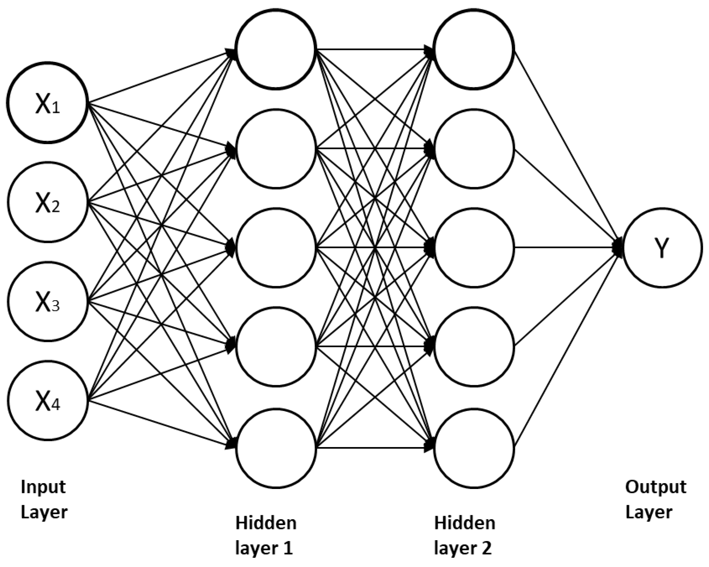
3.2.1. The Multi-Layer Perceptron (MLP)

Called also the multi-layer feed-forward neural network, the MLP is the first and simplest DL architecture. It consists of one input layer to receive the signal, one output layer that makes predictions about the input, and several hidden layers that are the true computational engine of the network. The number of neurons in each layer is variable and neurons are all fully connected. These networks are generally used for regression and classification problems, with a very large amount of training data [26]. The MLP architectures belong to the class of supervised learning algorithms and use the back-propagation for training. It is considered insufficient for advanced computer vision tasks. In fact, since each perceptron is connected with every other perceptron of the network, the total number of parameters can become very high. Another limitation of MLP is that it does not consider spatial information for prediction. It takes flattened vectors as inputs, thus predictions are made pixel by pixel. Figure 2 provides a representation of an MLP with two hidden layers.

3.2.2. The Convolutional Neural Networks (CNN)

To overcome the shortcomings of MLP networks in computer vision tasks, the CNN has been designed. It is a particular type of network used especially for data in 2D or for structures in more dimensions, such as images, videos, or sequences [22]. Its general operating principle is to apply successive convolution operations to the input data in order to automatically extract features (important characteristics) and reduce data sizes. In addition to input and output layers, the CNN network consists of four basic layers that include a convolution layer, pooling layer, flattening layer, and a fully connected layer [23]. The convolutional layers (considered as the core building blocks of the CNN) allow for extracting features from an input by mathematical operations such as the matrix and filter or kernel. The pooling layers (sometimes called subsampling or downsampling) reduce the dimension of each map but retain important information. The matrix are flattened into 1D vectors by the flattening layer and then information are fed into a fully connected layer. Unlike MLP architectures, layers are not fully connected in CNN.

3.2.3. The Recurrent Neural Network (RNN)

These are generally used when input data are sequential, such as in time series, sound, or natural language processing. RNN architectures are suitable for designing predictive models [12,27,28,29]. Indeed, this network includes a feedback loop, which allows for consideration of the information of the previous layers for predictions. However, there are two main issues that may occur during the application of RNN architectures: the problem of vanishing and exploding gradients [8,24]. To overcome these limitations, two variants of RNN have been developed: the long short-term memory (LSTM) [30,31] and, more recently, the gated recurrent unit (GRU) [32,33]. They are recurrent networks with memory units called “cell”. The LSTM architecture has three gates (input, output, and forget gate), while the GRU has the reset and update gates.

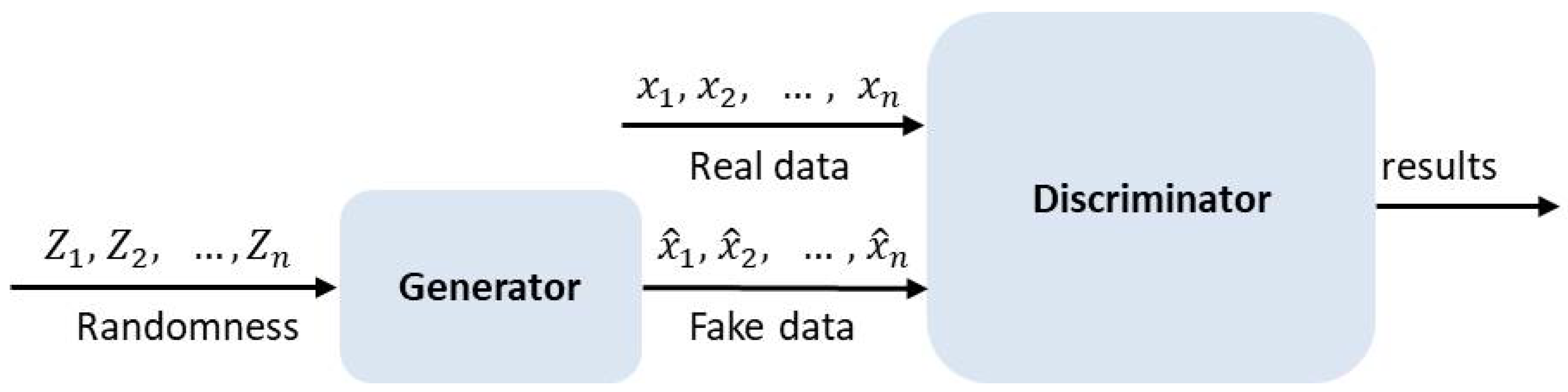
3.2.4. The Generative Adversarial Network (GAN)

This is a very famous architecture that has had impressive success since its creation [34]. The GAN model consists of two opposing networks (generator and discriminator) which oppose each other in order to generate an artificial instance of data strongly resembling that of the real one [34]. The generator aims to create new data received by the discriminator which determines whether they are true or generated due to a database made up of real data. Thus, the first network learns to create more and more realistic elements while the second learns to recognize real data in the best way.

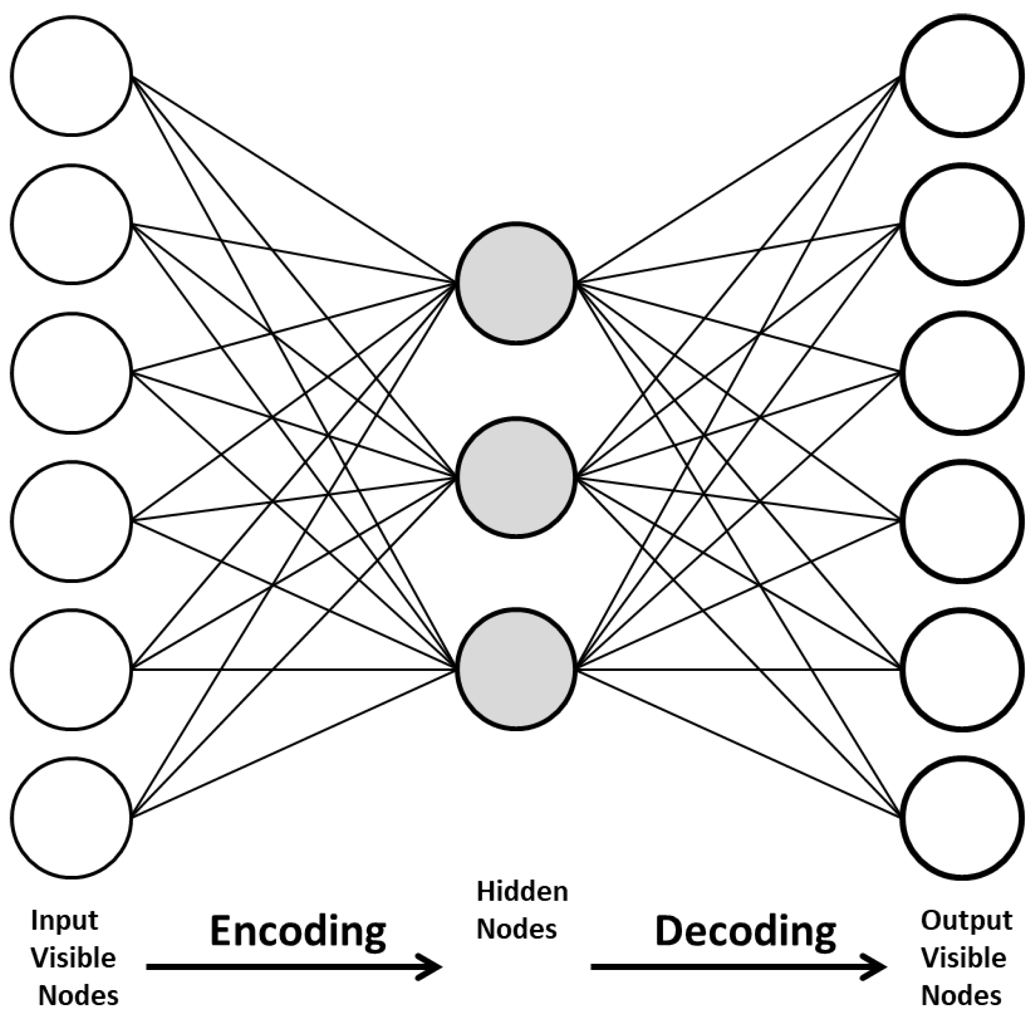
3.2.5. The Auto-Encoders (AE)

The AE are unsupervised algorithms able to deal with unlabeled data. The main objective of these architectures is to reduce the dimension of input variables in order to facilitate their processing and then learn how to reconstruct the same structure of input data for the output layer [35]. In the encoding stage, features are extracted and details are kept as much as possible. There are many variations of AE networks, such as the deep auto-encoder, denoising auto-encoder, contractive auto-encoder, variational auto-encoder, and sparse auto-encoder. They are generally used in association with other architectures. Recommendation systems, anomaly detection, dimension reduction, or image processing are some application cases of AE systems. Figure 3 presents a simple structure of an AE network.

4. Background on SITS

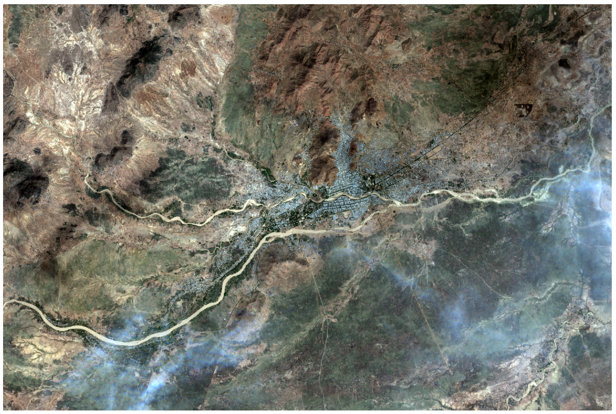
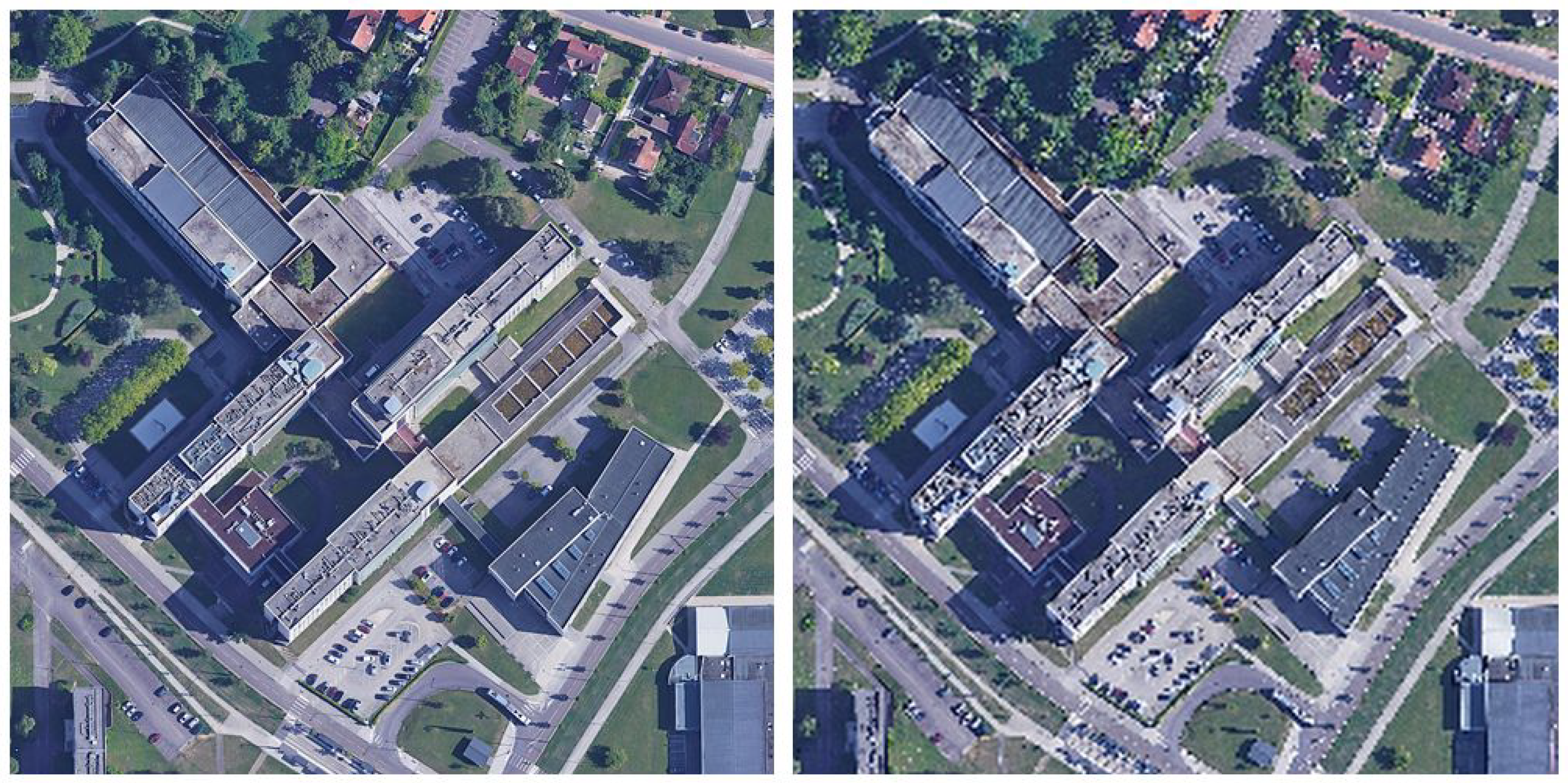
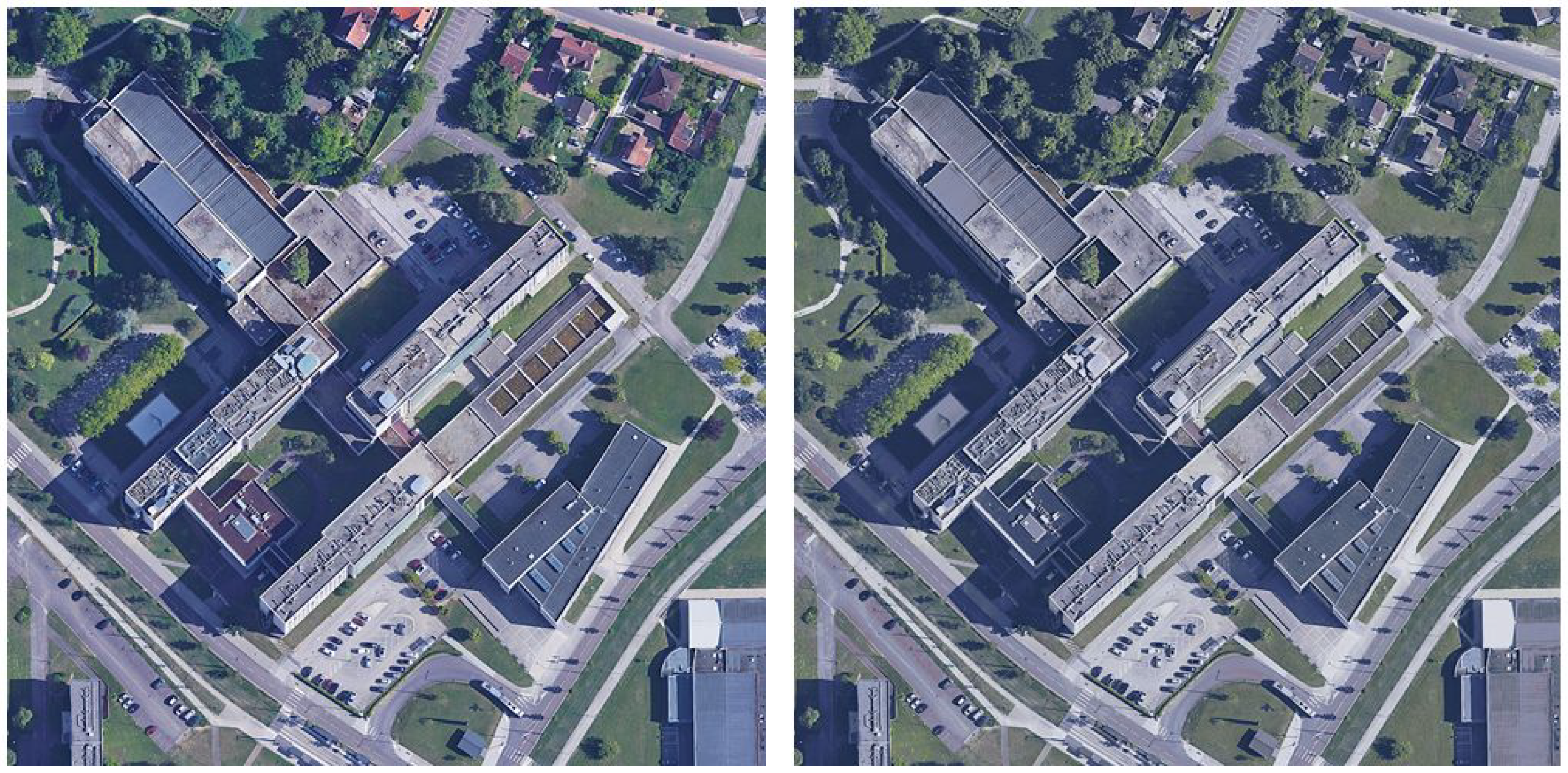
4.1. Description of Satellite Images

Remote sensing can be defined as all the techniques that allow for the acquiring of information about objects without direct contact with them. One of the most common types of remote sensing is remote sensing using satellites as a platform and producing information in the form of images. Today, more than 4000 satellites are orbiting around the Earth. Each satellite has its own sensor which gives specific data. They take pictures of the Earth at a given place and time. Thus, a satellite image (SI) or remote sensing image is an image representing a part of the Earth (or another planet) obtained from data recorded by a sensor installed on a satellite [2]. A list of operational satellites, with their characteristics and main objectives, is available on the satellite database of the Union of Concerned Scientists: https://www.ucsusa.org/resources/satellite-database (accessed on 25 August 2021).

Orbiting satellites carry calibrated sensors to detect various wavelengths along the electromagnetic spectrum, often including visible light. Systems are either active, where the source of energy is part of the sensor (Radar imaging), or passive, where the source of energy is the sun or Earth/atmosphere (optical imaging) [2,36]. Optical remote sensing generally covers the visible (VIS), near infrared (NIR), middle infrared (MIR), and thermal infrared (TIR) range of the electromagnetic spectrum. In near and middle infrared spectra, radiations are reflected like visible light, while thermal radiation is the heat energy emitted by the surface.

As opposed to optical systems, radar systems emit microwaves and measure the back scattered energy. The main advantage of radar systems is that they can take images regardless of the weather conditions or the time. Thus, radar images do not problems regarding cloudy images, like in optical systems, since microwaves pass through the cloud cover [36]. In practice, optical images are widely used and their interpretation as well as the data processing step are considered easier than for radar data. Indeed, the use of radar data for Earth observation is less intuitive and expertise is required to interpret images that look much less like a photo than optical images.

SI are specific data and differ from classical pictures in several respects:

• First, SI usually have many more pixels than a classical image considering that a photograph can already contain thousands of pixels;
• Second, SI and natural images do not have the same number of channels. Natural pictures have three channels: one for the red color, one for the green color, and one for the blue color (RGB). In addition to the three previous channels, SI can contain dozens of other channels; and
• Finally, SI are all geo-referenced.

All information about an SI, such as the resolution, number of channels, sun angle, atmospheric conditions, satellite position, etc., are recorded in the metadata file.

For example, Figure 4 represents the locality of Maroua in the Cameroon view from the satellite Sentinel 2. The image is in a true color (RGB) representation. One can observe the presence of a light cloud cover.

The resolution of images is an important characteristic to consider before choosing the suitable data for a specific project. In fact, there are three main types of resolutions:

• Spatial resolution: the size of the smallest element that can be observed by the sensor. Satellite image resolutions range from low to high and very high spatial resolution.
• Spectral resolution: refers to the bandwidth of each channel.
• Radiometric resolution: describes the ability to differentiate fine nuances in magnitudes of the electromagnetic energy (coding).
• Temporal resolution: the time between the acquisition of two images representing the same scene (satellite revisiting time).

Images with a high spatial resolution usually have low temporal resolution and vice versa. Figure 5 and Figure 6 illustrate the notions of the spatial and radiometric resolution of SI. One can observe in Figure 5 that the objects in the image with the smallest spatial resolution are more precise. Concerning the radiometric resolution (Figure 6), each pixel of the left image is coded on 8 bits, thus the image has more color than the right image.

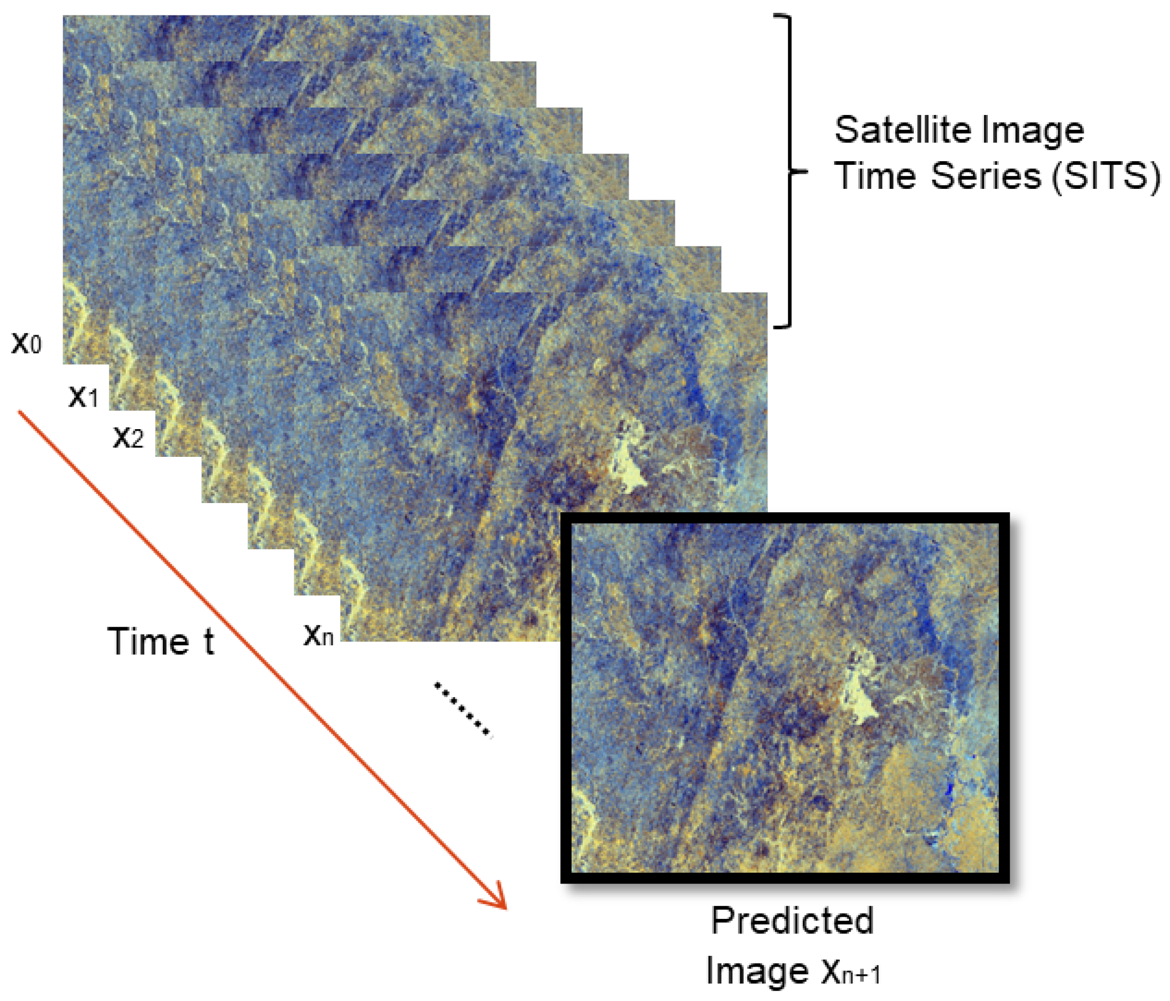
4.2. Description of the SITS Prediction Problem

Let $X_t$ be a satellite image representing a given area acquired at time t. A satellite image time series (SITS) is a sequence of images at different consecutive times [37]. Images may come from different sources but always represent the same scene. Thus, a SITS can be formulated by the series described in Equation (1):

$$SITS=X_1,X_2,\dots ,X_{t-1},X_t,\dots ,X_{t+1},\dots ,X_{t+n}$$

(1)

where $X_t$ represents the image X at time t.

When talking about Earth observation SITS, the term Earth observation data cube is widely used by scientists [38].

Prediction in SITS not only consists of the forecast future or unseen event. In some cases, it is related to data fusion or missing data reconstruction in sequences. When the predicted data concern future events, the term “forecasting” is generally used while the term “nowcasting” is used for very short-range forecasting. Overall, prediction problems in times series can be divided into three main types:

• “one-to-sequence”: from one input, the model generates many outputs. For instance, from one image provided as input, a sequence of words are generated as output (image captioning);
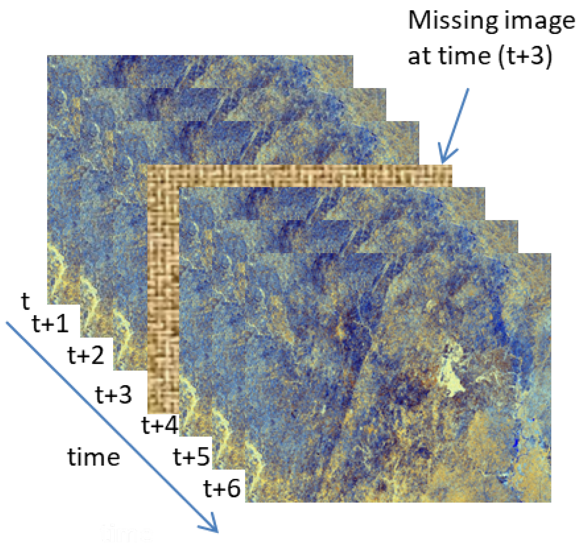
• “sequence-to-one”: here, inputs are a sequence and only one occurrence is produced as an output. That is, for example, the case of the next frame forecasting problem in time series, as illustrated in Figure 7; and
• “sequence-to-sequence”: in this case, both of the inputs and outputs are sequences, as in text translation tasks, for instance.

5. Major Applications of SITS Prediction Using DL

DL techniques are used for several types of SITS prediction problems. This paragraph presents the main applications mentioned in the literature.

5.1. Weather Forecasting

Weather forecasting tasks consist of predicting future conditions of the atmosphere (namely the temperature, humidity, and wind) for a given location and time. It is an important issue for disaster management. With the development of meteorological satellite technology, satellite cloud images allow for the characterization of the distribution of clouds on the image and are used to track the evolution of large-scale weather systems [39]. In addition to the classical numerical weather prediction (NWP) approach, DL techniques are used today by data scientists for weather forecasting and achieve more accurate results due to the availability of massive weather observation data and the advent of both information and computer technology [39]. Figure 8 illustrates the two concepts for weather forecasting: the theory-driven and the data-driven approaches. The theory-driven approach is focused on the understanding of physical mechanisms and uses NWP-based models for predictions, while the data-driven approach uses the spatial and temporal relationships between meteorological data and DL techniques. One can observe in the figure that the theory-driven method consists of three steps (data assimilation, execution of the NWP model, and visualization), while the data-driven approach directly uses data and DL algorithms to make predictions.

5.2. Precipitation Nowcasting

Precipitation nowcasting is an important and essential part of the weather forecasting problem. Its goal is to predict the future intensity of rain/snow in a local region over a relatively short period of time (e.g., 0–6 h) [40]. To achieve this goal, sequences of observed radar echo maps are used to forecast a fixed length of the future radar maps within a given area. Note that the radar echo maps are images which can be converted to rainfall intensity maps using the Marshall–Palmer relationship or Z–R relationship [41].

From the machine learning point of view, this problem is considered as a spatio-temporal sequence forecasting problem. Recently, studies have shown that DL techniques outperformed classical existing methods for precipitation nowcasting, namely NWP-based methods and radar-echo extrapolation-based methods. In fact, the availability of a huge amount of radar echo data and suitable models for end-to-end learning allow for achieving a better performance.

5.3. Spatio-Temporal Analysis

Spatio-temporal or spatial temporal analysis refers to the study of data collected across both space and time dimensions. It describes an event that occurred in a specific place over time. With the development of powerful computational processors, DL techniques are widely used nowadays by data scientists for spatio-temporal data analysis. Specific applications in SITS include the spatio-temporal prediction of snow cover [27], leaf area index [42], sea ice motion [43], vegetation [44], sea surface temperature [45], and others. In general, indices are first extracted from images before their use. In fact, map indices are images calculated from multi-channel images. They highlight a specific phenomenon that is present while mitigating other factors that alter the effects on the image. For example, a healthy vegetation is represented by a light color in the normalized difference vegetation index (NDVI) image, while unhealthy vegetation has lower values.

5.4. Missing Data Reconstruction

Earth observation imagery from remote sensing is one of the most important ways to obtain information of the surface of the Earth. Sometimes, because of some issues such as the internal malfunction of satellite sensors, the low temporal frequency, the poor atmospheric conditions, or other image-specific problems, the acquired satellite images suffer from missing information. For example, data can face the problem of dead pixels on images, thick cloud cover [46], or missing images in a temporal sequence, as in Figure 9. One can observe that in this illustration, according to the description of a SITS as given by Equation (1), the information of the image $X_{t+3}$ recorded at time $(t+3)$ are missing. Thus, the data usability is greatly reduced; it is thus necessary to reconstruct missing data in order to have complete sequence.

To date, several techniques for missing information reconstruction have been proposed. The approaches belong to four main categories, namely spatial based-methods, spectral-based methods, temporal-based methods, and spatio-temporal-spectral-based methods [46].

6. Deep Learning-Based Methods for SITS Prediction

The current part of this review presents the most DL-based approaches used for SITS prediction as well as some examples of their use in real-world problems. Models based on RNN, feed-forward networks, and hybrid architectures are reviewed, as well. Table 3 at the end of this section gives a summary of these methods.

6.1. RNN-Based Models

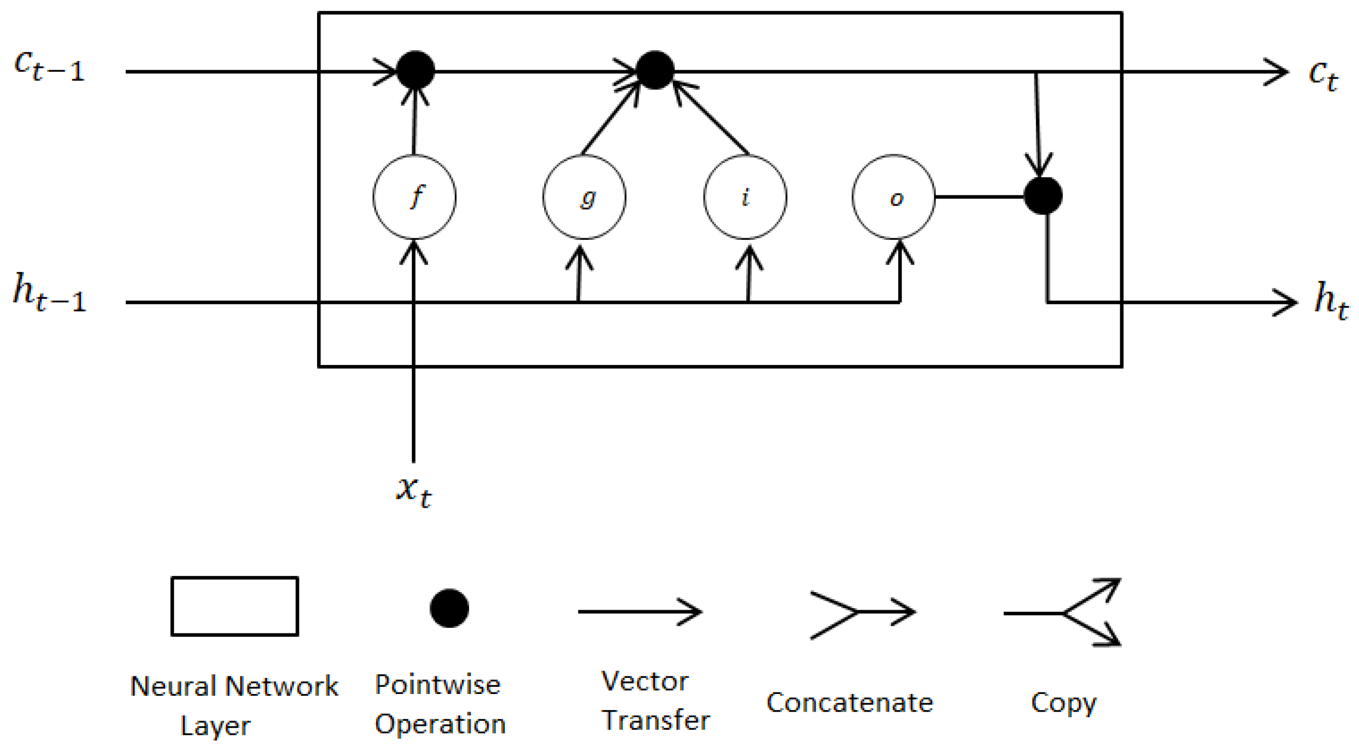
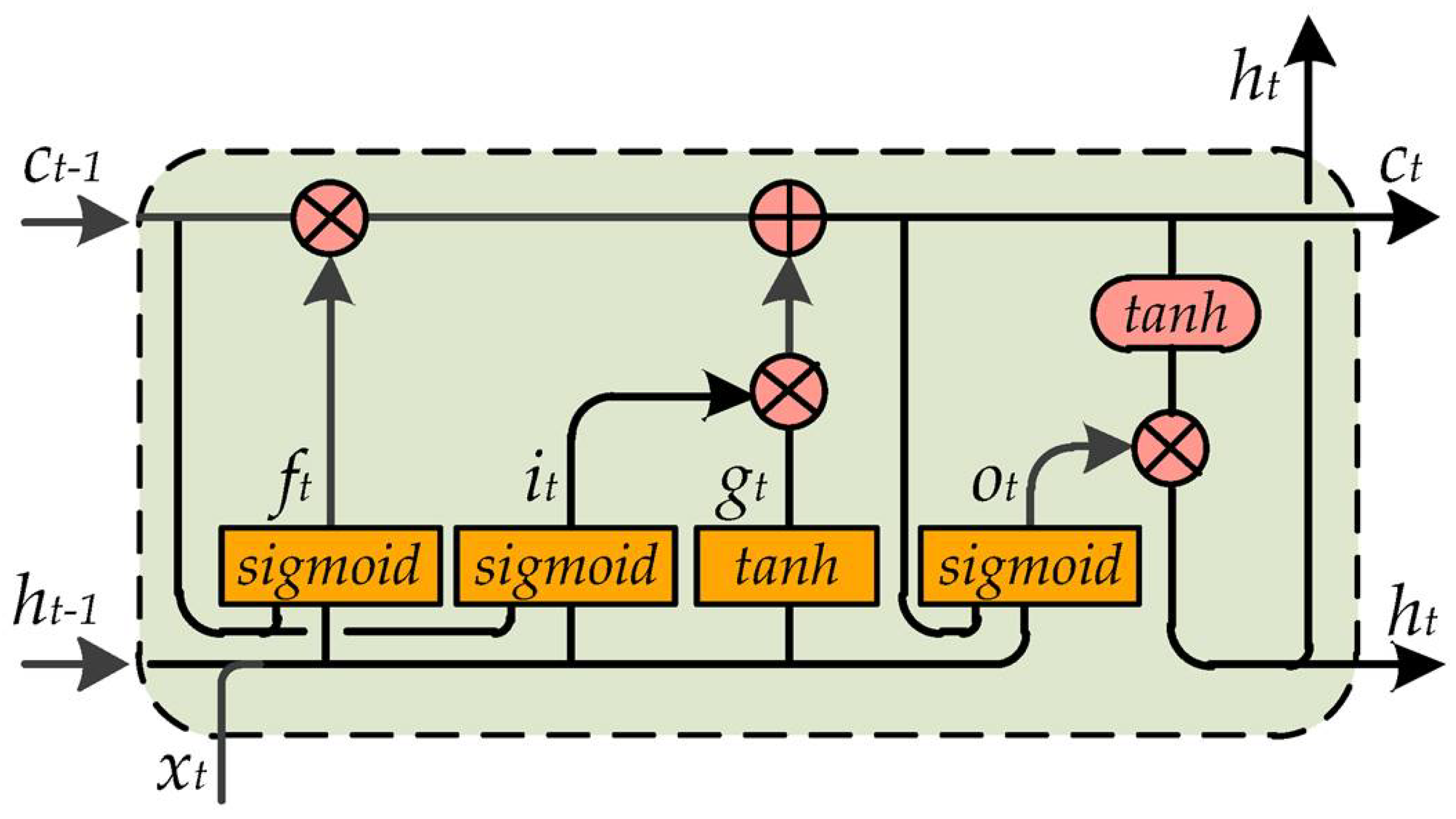
6.1.1. Long/Short-Term Memory

The LSTM network was designed to solve the problem of the vanishing gradient in RNN. Unlike that in standard recurrent networks, which have only one single activation layer, in LSTM architectures, there are four layers that interact in a special way: the information gate, forget gate, input gate, and output gate (note that in real configurations it may have more gates). Figure 10 shows the configuration of a simple LSTM memory block and Equations (2)–(7) describes each component in the memory block. One can observe that the LSTM block takes three data types as inputs.

$$c_t=f_t\odot c_{t-1}+i_t\odot g_t$$

(2)

$$h_t=o_t\odot {\sigma }_c\left(c_t\right)$$

(3)

$$i_t={\sigma }_g(W_i{x}_t+R_i{h}_{t-1}+b_i)$$

(4)

$$f_t={\sigma }_g(W_f{x}_t+R_f{h}_{t-1}+b_f)$$

(5)

$$g_t={\sigma }_c(W_g{x}_t+R_g{h}_{t-1}+b_g)$$

(6)

$${\sigma }_t={\sigma }_g(W_o{x}_t+R_o{h}_{t-1}+b_o)$$

(7)

where:

• $c_t$ and $h_t$ represent the cell state and hidden state at time t, respectively;
• $i_t$, $f_t$, and $o_t$ are the input, the forget, and the output gate at time t, respectively;
• $g_t$ is the cell candidate at time t;
• $x_t$ is the input vector to the LSTM unit;
• $W_{i,f,g,o}$ are the input weights for each component;
• $R_{i,f,g,o}$ represent the recurrent weight for each component;
• $b_{i,f,g,o}$ are the bias parameters for each component;
• ${\sigma }_c$ is the gate activation function (by default sigmoid);
• ${\sigma }_g$ defines the state activation function (by default tanh); and
• ⊙ is the Hadamart product.

Although the LSTM architectures are suitable for 1D data, some researchers have used this approach for SITS prediction. For example, the authors in [47] used a simple LSTM model for the reconstruction of daily missing pixels in optical images covered by cloud. In such a model, image predictions are done pixel by pixel. Since the obtained results were quite satisfactory, it has been concluded that LSTM networks are also usable for this kind of problem.

In a similar manner, multi-layer LSTM networks were used in [48] for sequence-to-sequence weather forecasting. Before the training step, some data were preprocessed. For example, missing values in a sequence were replaced by the last reordered value.

More recently, a new model based on thw LSTM architecture was presented in [49] for the Soybean yield prediction from satellite images and weather data. The authors compared the performance of their model with respect to the performance obtained by multivariate ordinary least squares (OLS) and random forest algorithms. After the analysis of the results obtained by each model, the authors concluded that satellite images combined with weather data can improve the accuracy of Soybean forecast models.

6.1.2. Convolutional LSTM

When solving prediction problems involving time series, RNN and particularly LSTMs are generally used for their ability to store the state from previous layers. However, this type of architecture was basically designed to work with one-dimensional data. For 2D data as images, the best approach is to use CNN-based models. Thus, in order to obtain good predictions using SITS, the capabilities of CNN and LSTM networks are merged to create the convolutional LSTM (ConvLSTM). In this architecture, matrix multiplication at each gate of classical LSTM is replaced with convolution operation and the input dimension of data is kept in the output layer instead of being just a one-dimensional vector. Figure 11 shows a representation of a simple memory block of the ConvLSTM architecture. On the basis of the LSTM block as represented by Figure 10, convolution operation is introduced in each input to capture spatial features. In the ConvLSTM architecture, all the attributes $X_t$, $C_t$, $h_t$, and the gates are 3D tensors [40].

The ConvLSTM architecture was introduced in 2015 by Xingjian shi et al. in [40]. The authors applied the proposed structure for solving a weather forecasting problem, namely the prediction of future precipitation intensities. For the same purposes, authors in [51] designed a new model called DeepRain based on the ConvLSTM architecture for precipitation forecasting using SITS. Models based on the ConvLSTM architecture are also used for other applications such as for the prediction of future satellite cloudage images or for the prediction of short and mid-term sea surface temperatures (described, respectively, in [45,52]).

In general, the results of research studies have shown that the ConvLSTM model outperformed main traditional models, namely the fully-connected LSTM (FC-LSTM), the real-time optical flow by variational methods for echoes of radar (ROVER) information, the linear regression method, and the MLP.

6.1.3. Trajectory-Gated Recurrent Unit (TrajGRU)

To overcome some limitations of ConvLSTM and Convolutional GRU (ConvGRU) models, the authors in [41] designed a new model and benchmark (dataset, training loss, and evaluation protocol) for precipitation nowcasting tasks. They designed a new TrajGRU model based on ConvGRU. It is able to actively learn the location-variant structure for recurrent connections. Unlike in classical convolutional RNN, recurrent connections are dynamically determined over time in the TrajGRU architecture [41], which is defined by Equations (8)–(12).

$$U_t,V_t=\gamma (X_t,H_{t-1})$$

(8)

$$Z_t=\sigma (W_{xz}\ast X_t+\sum _{l=1}^L{W}_{hz}^l\ast warp(H_{t-1},U_{t,l},V_{t,l}))$$

(9)

$$R_t=\sigma (W_{xr}\ast X_t+\sum _{l=1}^L{W}_{hr}^l\ast warp(H_{t-1},U_{t,l},V_{t,l}))$$

(10)

$$\begin{array}{c}\hfill H_t^{{}^{\prime }}=f(W_{xh}\ast X_t+R_t\circ (\sum _{l=1}^L{W}_{hh}^l\ast warp(H_{t-1},U_{t,l},V_{t,l})))\end{array}$$

(11)

$$H_t=(1-Z_t)\circ H_t^{{}^{\prime }}+Z_t\circ H_{t-1}$$

(12)

where:

• L represents the number of allowed links;
• $U_t,V_t\in {\mathbb{R}}^{L\times H\times W}$ denote the flow fields;
• $W_{hz}^l,W_{hr}^l,W_{hh}^l$ are the weights;
• $warp(H_{t-1},U_{t,l},V_{t,l})$ is the function that selects the positions pointed out by $U_{t,l},V_{t,l}$ from $H_{t-1}$;
• $H_t,R_t,Z_t,H_t^{{}^{\prime }}$ represent the memory gate, reset gate, update gate, and new information, respectively;
• $X_t$ is the input;
• f is the activation function; and
• ∘ denotes the Hadamart product.

Experimental results have shown that this new model was more efficient than the classical ConvGRU for precipitation nowcasting. However, to improve prediction accuracy in a realistic data context, some authors proposed a new sequence-to-sequence model based on TrajGRU, ConvGRU, and ConvLSTM [53].

6.2. Hybrid Models

For more complex problems, instead of using only one kind of architecture, scientists often combine two or more methods and expect better results. Sometimes, DL architectures are used in association with classical ML algorithms. Such models are called “hybrid models”. They refer to a category of methods which integrate the advantages of different individual models [54].

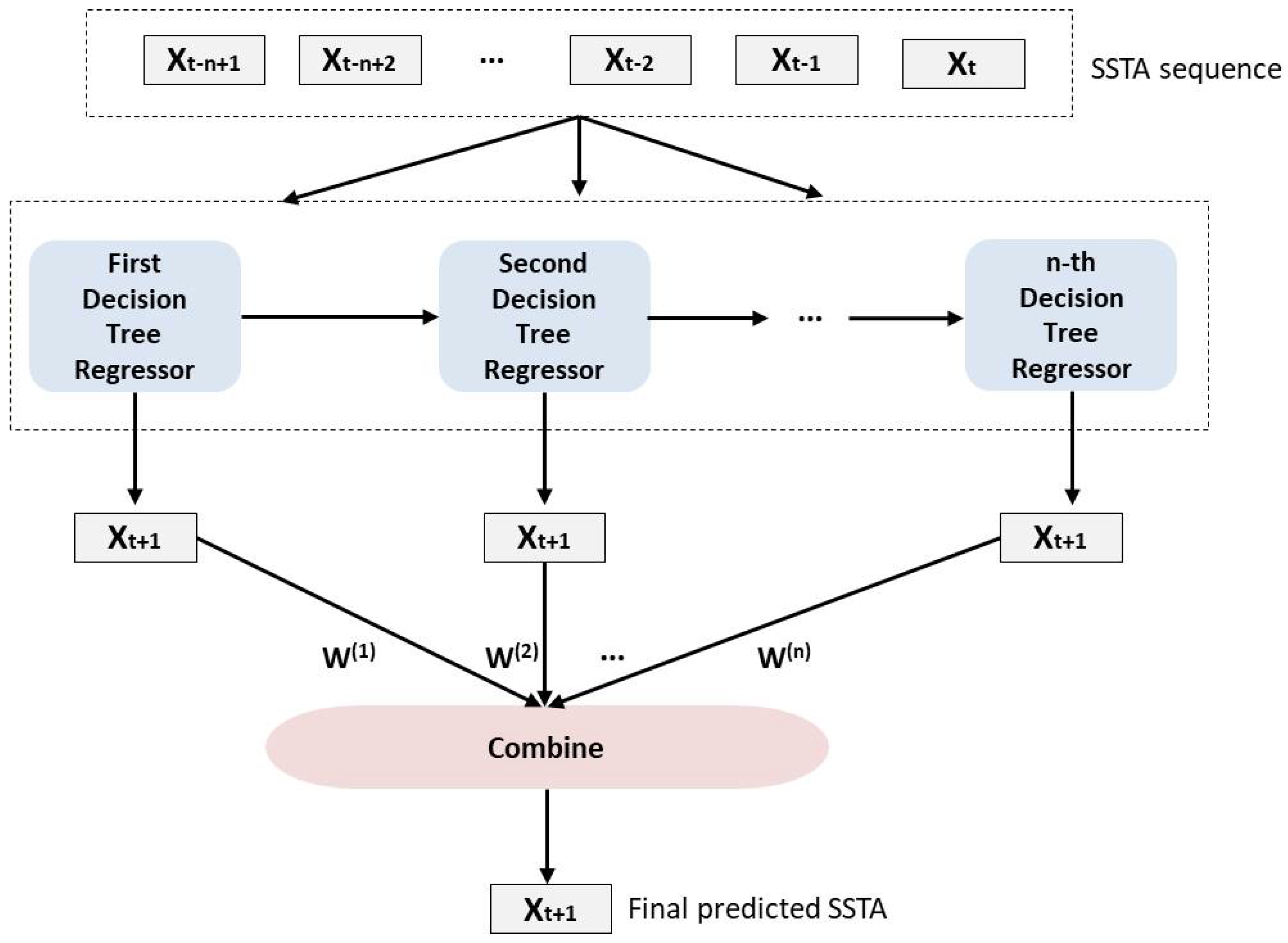
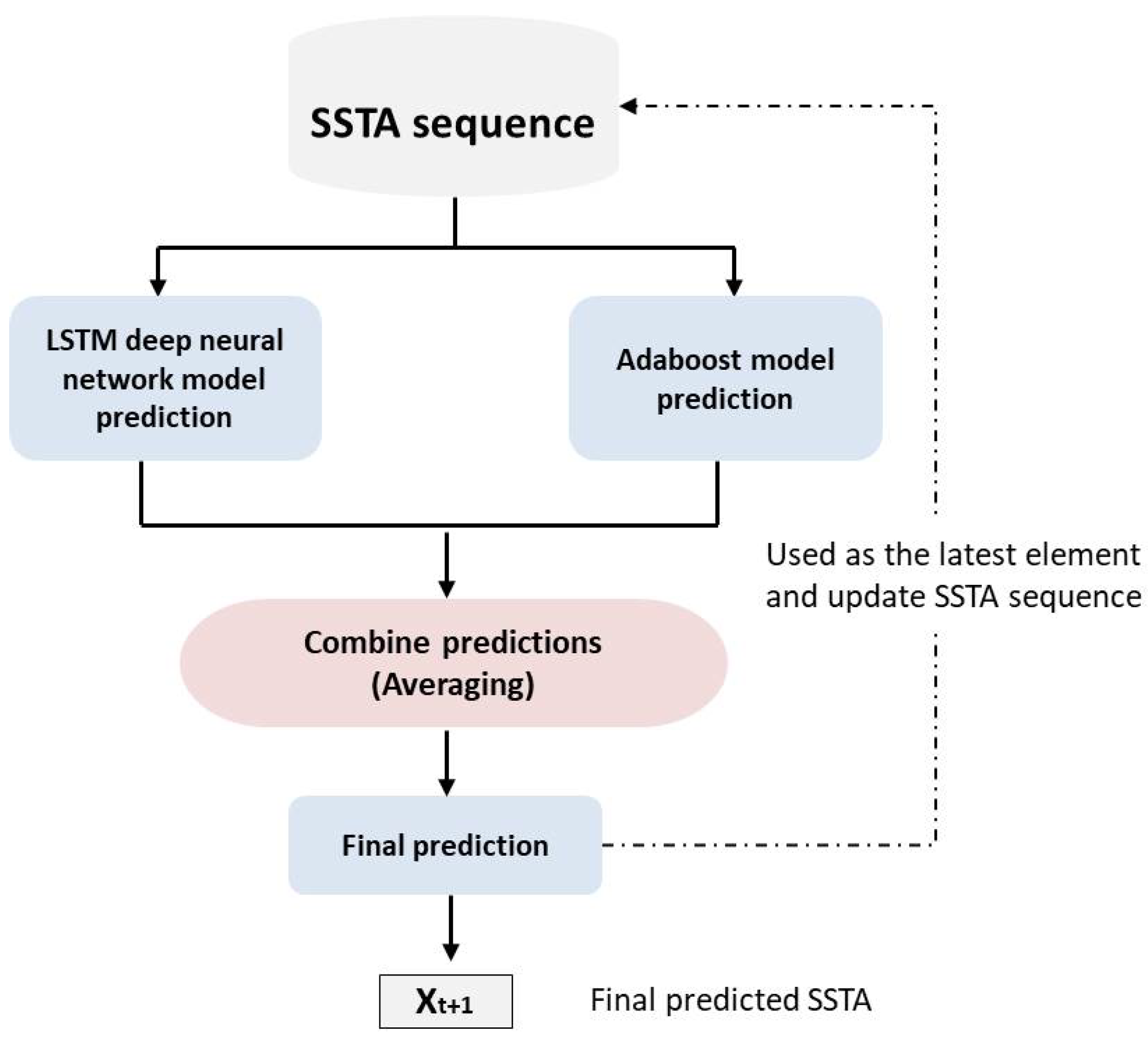
6.2.1. LSTM–AdaBoost

The LSTM–AdaBoost model was designed by Xiao et al. in [55] for the prediction of sea surface temperatures (SST). This model consists of the combination of two different types of architecture, namely the LSTM network and the adaptive boosting model (Adaboost).

AdaBoost is a boosting ML algorithm used as a classifier. It is generally used in combination with many other types of learning algorithms to improve performance. The term “adaptive boosting” is used because weights are re-assigned to each instance. It allocates more weight to hard-to-classify instances and less to those that are already well processed. This algorithm can be used for both regression and classification problems. The basic regressor boosted by AdaBoost as part of the LSTM–AdaBoost model is the decision tree regressor, which has been demonstrated to be powerful for predictions [55]. Figure 12 gives a simple representation of the AdaBoost part of the architecture. The top panel shows the generation of the boosted decision tree regressors. The weights for combining the predicted SSTAs are calculated during the boosting stage based on the produced prediction errors [55].

Before feeding data to this LSTM–AdaBoost network, data sequences need to be deseasonalized and normalized. Experimentation on short and mid-term future SST predictions have shown that the obtained results with the hybrid model outperformed those obtained with LSTM, Adaboost, or SVR (Support Vector Regression) separately. Note that concerning the issue of seasonal series, authors in [56] examined the question of whether the data should be deseasonalized first.

An overview of the whole LSTM–AdaBoost model is illustrated in Figure 13. The input SSTA sequence is first provided to both LSTM and AdaBoost networks for independent predictions. Then, each of their predictions are combined through averaging to produce the final prediction, which is used as the latest element of the input sequence [55].

6.2.2. Generative Adversarial Network–LSTM (GAN–LSTM)

The GAN–LSTM architecture consists of a combination of a supervised learning architecture with an unsupervised architecture, namely the LSTM and GAN networks, respectively. This method, as proposed in [57], combined the generator skills provided by the GAN and the forecast ability of the LSTM network for satellite image prediction. The GAN part of the model, which is represented by Figure 14, generated images from a set of random data. The generator was trained to fake the discriminator while the discriminator was trained to make the right judgment. Then, the LSTM part of the network provided some information for the hidden variable of the generator [57].

The main challenge to train a GAN model concerns the quality of generated images, which are supposed to be not only low in noise but also diverse. The training process of GAN and GAN–LSTM are detailed in Algorithms 1 and 2, respectively [57].

Algorithm 1 GAN Training Algorithm.

Require:$\alpha$, the learning rate; m, the batch size; and $n_D$, the number of iterations of the discriminator per generator iteration. Require:${\theta }_{d0}$, the initial discriminators parameters, and ${\theta }_{g0}$, the initial generators parameters.     for number of training iterations do       for $t=0$,…, $n_D$ do           sample ${\left\{x^{\left(i\right)}\right\}}_{i=1}^m\sim p_{data}$: a batch from the real data.           sample ${\left\{z^{\left(i\right)}\right\}}_{i=1}^m\sim p_z$: a batch from the noise prior.           $g_{\theta d}\leftarrow {\Delta }_{\theta d}\left[\frac{1}{m}{\sum }_{i=1}^m{L}_D(x^{\left(i\right)},z^{\left(i\right)};{\theta }_d,{\theta }_g)\right]$           ${\theta }_d\leftarrow {\theta }_d-\alpha .Optimizer({\theta }_d,g_{\theta g})$       end for       sample ${\left\{z^{\left(i\right)}\right\}}_1^m\sim p_z$: a batch from the noise prior.       $g_{\theta g}\leftarrow {\Delta }_{\theta g}\left[\frac{1}{m}{\sum }_{i=1}^m{L}_G(z^{\left(i\right)};{\theta }_d,{\theta }_g)\right]$       ${\theta }_g\leftarrow {\theta }_g-\alpha .Optimizer({\theta }_d,g_{\theta g})$     end for

Algorithm 2 GAN–LSTM Training Algorithm.

Require:$\alpha$, the learning rate, and m, the batch size. Require:${\theta }_{f0}$, the initial LSTM’s parameters.     Train GAN with Algorithm 1     Cut the generator $\left(G\right)$ of the trained GAN and attach it to the LSTM $\left(f_{lstm}\right).$     for number of training iterations do         sample ${\left\{v^{\left(i\right)}\right\}}_{i=1}^m\sim p_{data}$: a batch from the real data.         where $v^{\left(i\right)}={\stackrel{\sim }{v}}_{i-j+1},{\stackrel{\sim }{v}}_{i-j+2},\dots ,{\stackrel{\sim }{v}}_i$.         $g_{\theta f}\leftarrow {\Delta }_{\theta f}\left[\frac{1}{m}{\sum }_{i=1}^{m}MSE\right(G(f_{lstm}\left(v^{\left(i\right)}\right),{\stackrel{\sim }{v}}_{i+1}]$         ${\theta }_f\leftarrow {\theta }_f-\alpha .Optimizer({\theta }_f,g_{\theta f})$     end for

In a similar manner, in order to ameliorate the performance of the classical ConvGRU for precipitation nowcasting tasks, a hybrid architecture similar to the GAN–LSTM model was designed in [58]: the Generative Adversarial–ConvGRU (Ga–ConvGRU). The proposed model has two adversarial learning systems: a ConvGRU-based generator and a convolution neural network-based discriminator. The two systems of the model allow for more realistic and more accurate yield extrapolation [58].

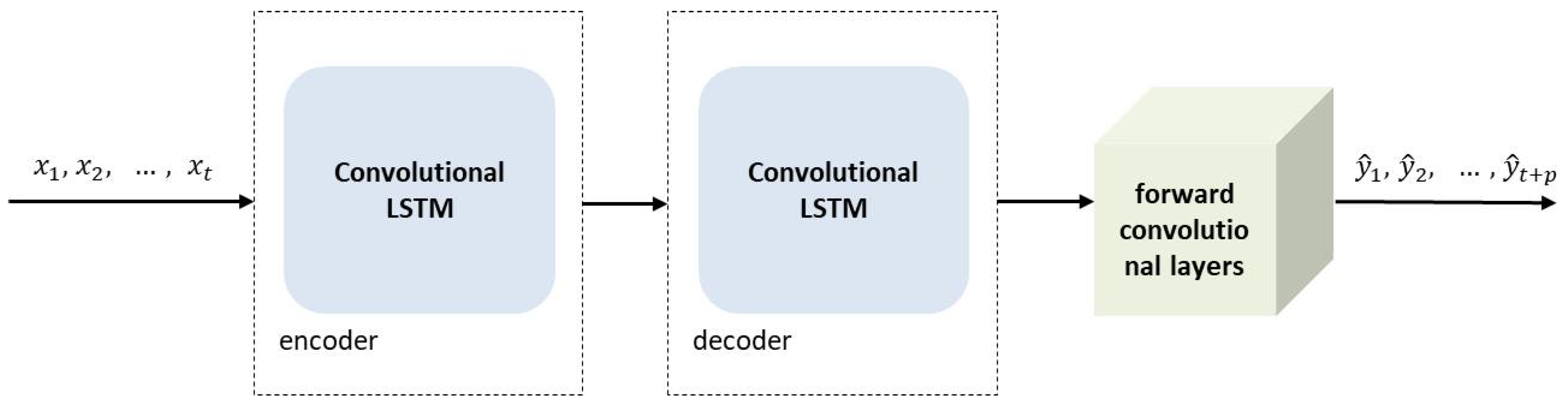
6.2.3. Convolutional LSTM Auto-Encoder

This architecture consists of two RNNs using an encoder–decoder framework. First, the encoder part of the model receives historical data and reduces information through time. Then, the encoded data and network states are used by the decoder to forecast values one by one. This approach was suggested, for example, in [59], to predict the next sequence of satellite images. To achieve better results, convolutional LSTM cells were introduced into both the encoder and the decoder. Since the quality of the predicted images in terms of resolution was not very good, the authors planned to improve the model by introducing a GAN into the model as a perspective to their study.

Similarly, a deep learning model composed of an encoder–decoder network with convolutional LSTM units was also proposed by authors in [43] for the prediction of future sea ice motion. The proposed model had an encoder–decoder structure with convolutional LSTM units. As shown in Figure 15, the last states and output cell of the encoder are copied to the decoder network. The encoder and decoder can consist of multiple layers of LSTM units stacked together, with the output of one layer being the input of the next one [43].

6.3. Feed-Forward-Based Models

6.3.1. DeepstepFE

The MLP or feed-forward multi-layer neural network is the first and simplest DL architecture. Numbers of neurons in each layer are variable and neurons are all fully connected. These networks are generally used for regression and classification problems, with a very large amount of training data.

Due to the presence of clouds on the optical images or the malfunctions that may occur on satellite engines, for example, data sequences are often incomplete. To solve the problem of missing data in a sequence of images, Monidipa Das and Soumaya Ghoh proposed in [60] a DL framework based on MLP architecture (DeepstepFE). The authors applied the model based on deep-step [44] for the reconstruction of missing NDVI images considering all available data (the previous and following images) in the sequence. The deep-step model was designed by the same authors in [44] and derived from the DSN model (deep stacking network).

According to the results obtained by the DeepstepFE model and by the other classical DL approaches for missing data prediction, the proposed DeepstepFE showed the best performance and had both a competitive and reasonable execution time.

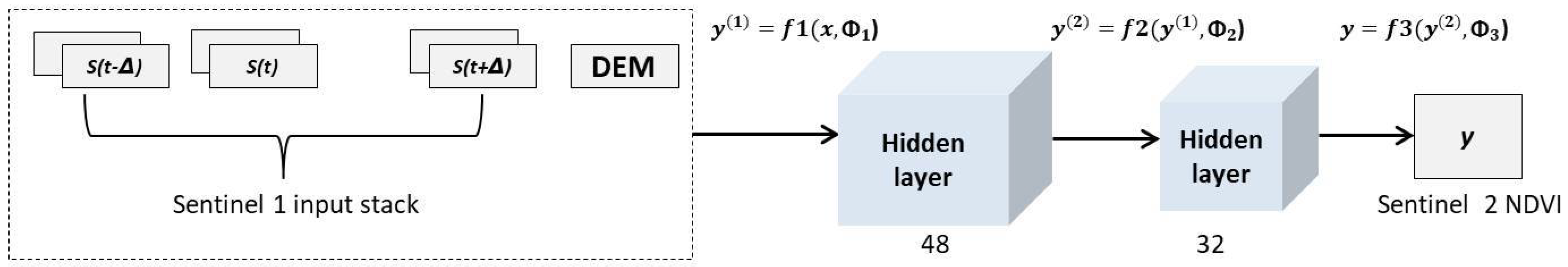
6.3.2. CNN-Based Approaches

To overcome the shortcomings of MLP networks in computer vision tasks, the CNN architecture has been designed by scientists. They are specially used for data in two or more dimensions. When working on image processing problems, the CNN consists of four basics layers: the convolution, pooling, flattening, and fully connected layer. Unlike MLP, layers are not fully connected in CNN. In SITS prediction problems, one can notice that the CNN is generally used for data fusion or missing data reconstruction.

For example, in [61], the authors explored the fusion of optical and radar images time series(Sentinel 2 and Sentinel 1) for the reconstruction of missing NDVI from synthetic aperture radar (SAR) data. To this end, they proposed a CNN-based model. The results of their study showed that there is a strong relationship between the radar data and the NDVI, which can be captured by a CNN model. The configuration of this architecture is presented in Figure 16. One can observe that the Sentinel 1 image time series, acquired every 12 days, passes through the CNN architecture, which outputs the corresponding Sentinel 2 NDVI image.

The overall CNN function is defined by Equation (13).

$$y=f(x,\Phi )=f_L(f_{L-1}(\dots f_1(x,{\Phi }_1),\dots ,{\Phi }_{L-1}),{\Phi }_L)$$

(13)

where $x=x^{\left(1\right)}$ is the input stack, $y=y^{\left(L\right)}$ is the estimated NDVI, and $\Phi \stackrel{\Delta }{=}({\Phi }_1,\dots ,{\Phi }_L)$ is the whole set of parameters to learn [61].

Another use case of the CNN is presented in [46] wherein a spatial–temporal–spectral framework based on CNN architecture is proposed for the reconstruction of missing data encountered in satellite images.Three main reconstruction tasks were considered in [46], namely the problem of dead lines in the Aqua MODIS band, the Landsat ETM + Scan Line Corrector (SCL)-off problem, and thick cloud removal. The Experimentatal results showed that the deep model performed well for the reconstruction of dead-lines in Aqua MODIS band 6. However, for the two other tasks, the authors encountered some limitations to solve in future works.

Table 3. Summary of the reviewed DL-based methods for SITS prediction. FF = feed-forward; TS-X = TERRA SAR-X; SP4-5 = SPOT4-5; F-2 = FORMOSAT-2; S1, S2 = Sentinel 1, 2; Corr. = correlation; and OA = overall accuracy.

Method Class	Ref.	Architecture	Dataset	Weakness	Advantage	Result
FF	[46]	CNN	MODIS and Landsat 7	Presence of spectral distortion and blurring	Use of multi-source data	$CC=0.97$
	[61]	CNN	S1 and S2	Presence of residual blur	Use of multi-source data	$SSIM=0.59$
	[62]	CNN	MODIS	Necessity to choose data for input	Accurate predictions	$RMSE=0.81$
	[60]	MLP	Landsat 7	Not working with raw satellite imagery	Use of the earlier and subsequent data	$PSNR=31.70$
	[44]	MLP	Landsat 7	Needs to create the NDVI map first	Good execution time	2118 seconds
	[63]	FFNN	TS-X, SP4-5, F-2, and RSAT2	Does not perform well on optical images	Use of multi-source data	$RMSE=7.00$
	[64]	FFNN	Meteosat 7	Not optimal for operational uses	High prediction accuracy	$RMSE=6.66$
RNN	[47]	LSTM	MODIS	Depends on the time of day	Accurate predictions	$R^2=0.90$
	[49]	LSTM	MODIS	Depends on weather conditions	Can be applied to other regions	$RMSE=0.68$
	[51]	ConvLSTM	Radar echo	Can not perform many-to-many prediction	Applied on four-channel data	$RMSE=11.31$
	[40]	ConvLSTM	Radar echo	Not suitable for long series	Accurate predictions of future rainfull	$Corr.=0.908$
	[45]	ConvLSTM	OISST2	Adapted to restricted cases	Can capture both the spatial and temporal correlations	$R=0.99$
	[52]	ConvLSTM	FY-2Y	Blur effect on the predicted images	Good accuracy	$SSIM=0.98$
	[53]	Radar echo	ConvGRU and TrajGRU	Needs to be trained several times	Cheap and effective solution	$SSIM=0.52$
Hybrid	[55]	LSTM–Adaboost	AVHRR	Series need to be deseasonalized first	Less overfitting	$MAE$: $+3.73\%$
	[65]	ConvGRU–CNN	S1 and S2	Requires many radar images	Transferable to other study areas	$OA=91.03$
	[57]	GAN–LSTM	FY-2F	Only one channel of the images is considered	Robust solution	$CR=0.78$
	[25]	ESS–MLP	Radar echo	Many steps before predictions	Good accuracy	$R^2=0.9$
	[43]	CNN–LSTM	AMSR E2	Only one channel of the images is considered	Can perform predictions several days in the future	$xRMSE=4.2$
	[42]	RNN–NARX	HJ-1A/1BCCD	Needs to create the index map first	Robust solution	$R^2=0.88$
	[66]	RNN–LSTM	Radar echo	Tested on small images	Performs well on videos	$MSE=44.2$
	[59]	ConvLSTM–AE	COMS1	Resolution of predicted images is not good	Predicts unseen weather situations	$MSE=197.2$

Table 3. Summary of the reviewed DL-based methods for SITS prediction. FF = feed-forward; TS-X = TERRA SAR-X; SP4-5 = SPOT4-5; F-2 = FORMOSAT-2; S1, S2 = Sentinel 1, 2; Corr. = correlation; and OA = overall accuracy.

Method Class	Ref.	Architecture	Dataset	Weakness	Advantage	Result
FF	[46]	CNN	MODIS and Landsat 7	Presence of spectral distortion and blurring	Use of multi-source data	$CC=0.97$
	[61]	CNN	S1 and S2	Presence of residual blur	Use of multi-source data	$SSIM=0.59$
	[62]	CNN	MODIS	Necessity to choose data for input	Accurate predictions	$RMSE=0.81$
	[60]	MLP	Landsat 7	Not working with raw satellite imagery	Use of the earlier and subsequent data	$PSNR=31.70$
	[44]	MLP	Landsat 7	Needs to create the NDVI map first	Good execution time	2118 seconds
	[63]	FFNN	TS-X, SP4-5, F-2, and RSAT2	Does not perform well on optical images	Use of multi-source data	$RMSE=7.00$
	[64]	FFNN	Meteosat 7	Not optimal for operational uses	High prediction accuracy	$RMSE=6.66$
RNN	[47]	LSTM	MODIS	Depends on the time of day	Accurate predictions	$R^2=0.90$
	[49]	LSTM	MODIS	Depends on weather conditions	Can be applied to other regions	$RMSE=0.68$
	[51]	ConvLSTM	Radar echo	Can not perform many-to-many prediction	Applied on four-channel data	$RMSE=11.31$
	[40]	ConvLSTM	Radar echo	Not suitable for long series	Accurate predictions of future rainfull	$Corr.=0.908$
	[45]	ConvLSTM	OISST2	Adapted to restricted cases	Can capture both the spatial and temporal correlations	$R=0.99$
	[52]	ConvLSTM	FY-2Y	Blur effect on the predicted images	Good accuracy	$SSIM=0.98$
	[53]	Radar echo	ConvGRU and TrajGRU	Needs to be trained several times	Cheap and effective solution	$SSIM=0.52$
Hybrid	[55]	LSTM–Adaboost	AVHRR	Series need to be deseasonalized first	Less overfitting	$MAE$: $+3.73\%$
	[65]	ConvGRU–CNN	S1 and S2	Requires many radar images	Transferable to other study areas	$OA=91.03$
	[57]	GAN–LSTM	FY-2F	Only one channel of the images is considered	Robust solution	$CR=0.78$
	[25]	ESS–MLP	Radar echo	Many steps before predictions	Good accuracy	$R^2=0.9$
	[43]	CNN–LSTM	AMSR E2	Only one channel of the images is considered	Can perform predictions several days in the future	$xRMSE=4.2$
	[42]	RNN–NARX	HJ-1A/1BCCD	Needs to create the index map first	Robust solution	$R^2=0.88$
	[66]	RNN–LSTM	Radar echo	Tested on small images	Performs well on videos	$MSE=44.2$
	[59]	ConvLSTM–AE	COMS1	Resolution of predicted images is not good	Predicts unseen weather situations	$MSE=197.2$

7. Optimizer and Evaluation Metrics Used for SITS Prediction

Depending on the problem, different elements are used for prediction in SITS. This section presents the optimizers and the performance metrics used in the reviewed studies.

Table 4 gives an overview of these elements according to the studied field.

7.1. Optimizer

During the learning step in neural networks, special methods or algorithms called optimizers are used to minimize the difference between the predicted output and the real one. This optimization is made by the readjustment or update of weights in order to obtain the most accurate predictions. In the literature, several types of optimizers exist and the choice of the most suitable algorithm for a DL model is crucial.

Gradient descent is one of the most popular algorithms to perform optimization and the most common way to optimize neural networks. There are three basic kinds of variants of gradient descent depending on the amount of data used for the gradient descent: batch gradient descent, stochastic gradient descent (SGD), and mini-batch gradient descent. Although SGD proved itself as an efficient and effective optimization method for DL algorithms, there are some variants that have been introduced, namely the adaptive moment (Adam) and the root mean square propagation (RMSProp) [67,68]. In the reviewed studies, the aforementioned SGD, Adam, and RMSProp algorithms have been used to train models.

7.1.1. The Stochastic Gradient Descent (SGD)

In the SGD, all the parameters are updated for each occurrence individually instead of computing the gradient of the cost function for the entire training dataset. The core of this approach is to minimize a function that can be written as the sum of differentiable functions. It is suitable for unconstrained optimization problems and has proven to be very effective in a variety of deep neural networks [44,46,49].

Equation (14) describes the SGD update rule.

$$W_{k+1}=W_k-\eta \Delta J\left(W_k\right)$$

(14)

where $W_{k+1}$ is the updated value after the k-th iteration, $W_k$ is the initial value before the k-th iteration, $\eta$ is the step size, and $\Delta J$ is the gradient of J.

7.1.2. The Root Mean Square Propagation (RMSProp)

The RMSProp function developed by Geoffrey Hinton is usually a suitable choice for RNN [43,58].

In the RMSProp algorithm, the learning rate for each parameter is automatically adjusted by an exponentially decaying average of squared gradients. The author of the RMSProp suggests to set the default value for the learning rate to $\eta =0.001$.

Equations (15) and (16) define the RMSProp optimizer.

$$E\left[g^2\right]\left(t\right)=\beta E\left[g^2\right](t-1)+(1-\beta ){(\frac{\delta c}{\delta w})}^2$$

(15)

$$w_{ij}\left(t\right)=w_{ij}(t-1)-\frac{\eta }{\sqrt{E\left[g^2\right]}}\frac{\delta c}{\delta w_{ij}}$$

(16)

where $E\left[g\right]$ is the moving average of squared gradients, $\frac{\delta c}{\delta w}$ is the gradient of the cost function with respect to the weight, $\eta$ is the learning rate, and $\beta$ is the moving average parameter.

7.1.3. The Adaptive Moment (Adam)

The Adam optimizer is by far one of the most preferred optimizers for DL algorithms. This algorithm of estimation combines capabilities of both the RMSProp and Momentum optimizers [69]. In the literature, most studies use the Adam optimizer for SITS prediction. In fact, the Adam optimizer is simple to implement, computationally efficient, require little memory and tuning, and is appropriate for problems with very noisy or sparse gradients.

The Adam function is defined by Equations (17)–(20).

$$v_t={\beta }_1\ast v_{t-1}-(1-{\beta }_1)\ast g_t$$

(17)

$$s_t={\beta }_2\ast s_{t-1}-(1-{\beta }_2)\ast g_t^2$$

(18)

$$\Delta w_t=-\eta \frac{v_t}{\sqrt{s_t+ϵ}}\ast g_t$$

(19)

$$w_{t+1}=w_t+\Delta w_t$$

(20)

where:

• $\eta$ denotes the initial learning rate;
• $g_t$ is the gradient at time t;
• $v_t$ represents the exponential average of the gradient;
• $s_t$ represents the exponential average of the square of the gradient;
• ${\beta }_1$ and ${\beta }_2$ are hyperparameters; and
• and each parameter $w^j$ is replaced by w for more clarity.

7.2. Evaluation Metrics

The choice of the appropriate evaluation metrics for models is a crucial step for any DL project. In fact, depending on the used metric, the evaluated model may or may not provide satisfying results. It is therefore very important to test multiple measures. In the literature, different metrics are tested to evaluate models. One can classify these measures in six main groups:

7.2.1. Regression Metrics

In most of the reviewed publications, one can observe that at least one of the following regression metrics is used for the evaluation of the designed models: the mean squared error (MSE), the mean absolute error (MAE), and the coefficient of determination (equivalent to the square of the Pearson correlation coefficient $R^2$). In fact, these metrics are considered to be the best for the evaluation of regression models. In addition, some derived versions, such as root mean square error (RMSE), mean absolute percentage error (MAPE), normalized-RMSE, and normalized mean bias error (nMBE), are also used to evaluate the performance of the models. More details on regressions metrics are in [70].

7.2.2. Computer Vision Metrics

The following metrics, generally used in computer vision problems, have been chosen by some authors: the peak signal-to-noise ratio (PSNR), the structural similarity index (SSIM), the spectral angle mapper (SAM), and the difference image (DI) [46,47,60,61].

The PSNR calculates the peak signal-to-noise ratio in decibels between two images. Its goal is to evaluate the quality between the original and the compressed image by the ratio value. The higher the PSNR, the better the quality of the reconstructed image.

With regard to the SSIM index, this allows for measuring the structural similarity between the predicted images and original ones. Values close to 1 indicate good similarities.

Regarding the SAM, this is based on a physical concept that measures the angular similarity between the spectrum of each pixel of the image and the reference spectra. Finally, the DI results from the subtraction operations between the values of each pixel of the input image and the values of the pixels corresponding to the predicted image. A dark DI with values close to 0 indicates that the prediction is good.

Table 4. Optimizer and categories of evaluation metrics used in the reviewed studies. Ref.: reference; NA: not available; CV: computer vision; Class.: classification; Proc.: processing; Prop.: proposed; Regres.: regression; and Stat.: statistical.

Prediction Domain	Ref.	Dataset	Architecture	Optimizer			Categories of Evaluation Metrics
				Adam	RMSProp	SGD	Class.	CV	Proc.	Prop.	Regres.	Stat.
Missing data	[65]	Sentinel 1 and Sentinel 2	ConvGRU + CNN	NA	NA	NA	√
	[46]	MODIS and Landsat 7	CNN			√		√				√
	[61]	Sentinel 1 and Sentinel 2	CNN	NA	NA	NA		√				√
	[60]	Landsat 7	Deep MLP	NA	NA	NA		√	√		√
	[47]	MODIS	LSTM	√				√			√
Precipitation	[53]	Radar echo	ConvLSTM, Conv, and Traj–GRU	NA	NA	NA						√
	[51]	Radar echo	ConvLSTM	√							√
	[40]	Radar echo	ConvLSTM	NA	NA	NA					√	√
	[58]	Radar echo	GAN + ConvGRU	NA	NA	NA						√
	[48]	Radar echo	LSTM	√						√	√
	[64]	Meteosat 7	Deep FFNN	NA	NA	NA					√	√
	[25]	Radar echo	SOM and ESS + MLP	NA	NA	NA					√
Spatio-temp	[45]	OISST2	ConvLSTM	√							√	√
	[44]	Landsat 7	Deep MLP			√			√		√
	[43]	AMSR E-2	CNN + LSTM		√				√		√
	[42]	HJ-1A/1B CCD	RNN + NARX	NA	NA	NA					√	√
	[27]	MODIS	RNN + NARX	NA	NA	NA					√	√
	[66]	Radar echo	RNN + LSTM	√					√		√
Weather	[59]	COMS-1	ConvLSTM + AE	√							√
	[57]	FY-2F	GAN + LSTM	NA	NA	NA
	[52]	FY-2F	ConvLSTM	√				√		√	√
	[55]	AVHRR	AdaBoost + LSTM	NA	NA	NA					√
Crop yield	[62]	MODIS	CNN	NA	NA	NA					√
	[49]	MODIS	LSTM			√					√
	[63]	T.SAR-X and FORMOSAT2	Deep FFNN	NA	NA	NA					√

Table 4. Optimizer and categories of evaluation metrics used in the reviewed studies. Ref.: reference; NA: not available; CV: computer vision; Class.: classification; Proc.: processing; Prop.: proposed; Regres.: regression; and Stat.: statistical.

Prediction Domain	Ref.	Dataset	Architecture	Optimizer			Categories of Evaluation Metrics
				Adam	RMSProp	SGD	Class.	CV	Proc.	Prop.	Regres.	Stat.
Missing data	[65]	Sentinel 1 and Sentinel 2	ConvGRU + CNN	NA	NA	NA	√
	[46]	MODIS and Landsat 7	CNN			√		√				√
	[61]	Sentinel 1 and Sentinel 2	CNN	NA	NA	NA		√				√
	[60]	Landsat 7	Deep MLP	NA	NA	NA		√	√		√
	[47]	MODIS	LSTM	√				√			√
Precipitation	[53]	Radar echo	ConvLSTM, Conv, and Traj–GRU	NA	NA	NA						√
	[51]	Radar echo	ConvLSTM	√							√
	[40]	Radar echo	ConvLSTM	NA	NA	NA					√	√
	[58]	Radar echo	GAN + ConvGRU	NA	NA	NA						√
	[48]	Radar echo	LSTM	√						√	√
	[64]	Meteosat 7	Deep FFNN	NA	NA	NA					√	√
	[25]	Radar echo	SOM and ESS + MLP	NA	NA	NA					√
Spatio-temp	[45]	OISST2	ConvLSTM	√							√	√
	[44]	Landsat 7	Deep MLP			√			√		√
	[43]	AMSR E-2	CNN + LSTM		√				√		√
	[42]	HJ-1A/1B CCD	RNN + NARX	NA	NA	NA					√	√
	[27]	MODIS	RNN + NARX	NA	NA	NA					√	√
	[66]	Radar echo	RNN + LSTM	√					√		√
Weather	[59]	COMS-1	ConvLSTM + AE	√							√
	[57]	FY-2F	GAN + LSTM	NA	NA	NA
	[52]	FY-2F	ConvLSTM	√				√		√	√
	[55]	AVHRR	AdaBoost + LSTM	NA	NA	NA					√
Crop yield	[62]	MODIS	CNN	NA	NA	NA					√
	[49]	MODIS	LSTM			√					√
	[63]	T.SAR-X and FORMOSAT2	Deep FFNN	NA	NA	NA					√

7.2.3. Statistical Metrics

These metrics are generally used in statistic or probability problems. The false alarm rate (FAR), the probability of detection (POD), the critical success index (CSI), the heidke skill score (HSS), the correlation coefficient (CC), and the Pearson correlation are statistical metrics computed to evaluate the performance of proposed DL-based models for SITS prediction. The POD, FAR, and CSI metrics, which are the most commonly used by authors in the literature, are defined by the following equations:

$$POD=\frac{TP}{TP+FP}$$

(21)

$$FAR=\frac{FN}{TP+FN}$$

(22)

$$CSI=\frac{TP}{TP+FP+FN}$$

(23)

where $TP$, $FP$, and $FN$ represent the number of true-positive predictions, the number of false-positive predictions, and the number of false-negative predictions, respectively.

7.2.4. Processing Metrics

In addition to classical measures used in DL problems, some authors recorded other values such as the model’s training time, the execution time, or the computer memory consumption during the training step. These values, in this paper, are called “processing metrics”. They have been used in [43,44,66].

7.2.5. Classification Metrics

To evaluate the performance of the data fusion model, authors in [65] used the commonly employed measures appropriate for classification problems (accuracy, Kappa, and f-measure).

7.2.6. Proposed Metrics

In [48,52], authors proposed new evaluation metrics and obtained a better performance compared to those obtained with classical ones.

8. Limitations in the Use of DL for SITS Prediction

Deep learning techniques are used today in most real-life applications and the remote sensing domain is not an exception. However, studies regarding the use of DL algorithms for SITS are still recent and present some particular challenges. This section summarizes the major factors that limit the use of DL for SITS prediction.

8.1. Limits Related to Training Dataset Availability

It is necessary to use a large training dataset to obtain satisfactory results with DL algorithms. However, contrary to models that use conventional images, there is a significant lack of labeled remote sensing data. Even if some training datasets are available for the remote sensing community, the problem regarding the quantity of elements in these databases persists. This issue of limited training samples is more important for working with Earth observation SITS. It is important to constitute a long time series of images to achieve accurate predictions [71].

There are several satellite missions that provide a large quantity of data. However, the collection and preprocessing of remote sensing images to build a usable dataset for SITS prediction is not a simple task [38]. In addition, Earth observation images are complex and varied (particularly because of the geographical metadata). The images are large, unlike traditional imagery datasets that are constituted of relatively small amounts of data. Thus, the download and storage costs are two aspects that make data availability difficult [71]. Considering there is a lack of preprocessed training datasets for SITS prediction, other types of images are often used for model validation in the literature. These include, for example, the MNIST, the Moving MNIST, and the KTH Action databases. Low resolution images such as meteorological series and radar echo datasets are, therefore, most often used in the domain of SITS prediction. To solve this problem, scientists are encouraged to publish methods and algorithms for downloading automatic Earth observation images. Databases of preprocessed SITS should also be made public to facilitate and promote experimentation.

Table 5. List of the main free tools used for SITS processing. GIS = geographic information system.

Tool	Description	Hyperlink
MAJA (MACCS ATCOR Joint Algorithm)	A cloud detection and atmospheric correction chain. It is adapted to the processing of high resolution image time series.	https://logiciels.cnes.fr/fr/node/57?type=desc (accessed on 3 November 2021)
OTB (Orfeo toolbox)	An open-source project for state-of-the-art remote sensing.	https://www.orfeo-toolbox.org/ (accessed on 3 November 2021)
Monteverdi	A satellite image viewer.	https://www.orfeo-toolbox.org/CookBook/Monteverdi.html (accessed on 3 November 2021)
SNAP (Sentinel Application Platform)	A software for Sentinel image processing.	http://step.esa.int/main/download/ (accessed on 3 November 2021)
NEST (Next ESA SAT Toolbox)	A software for the processing and analysis of radar and optical spatial data.	http://step.esa.int/main/ (accessed on 3 November 2021)
Emmah tools	A tool for image validations.	https://www6.paca.inrae.fr/emmah/ (accessed on 3 November 2021)
ILWIS (Integrated Land and Water Information System)	A remote sensing and GIS software that integrates image, vector, and thematic data in one unique and powerful package.	http://52north.org/communities/ilwis (accessed on 3 November 2021)
ImageJ	A tool for SI processing and analysis in Java.	http://rsbweb.nih.gov/ij/ (accessed on 3 November 2021)
GRASS GIS (Geographic Resources Analysis Support System)	A GIS technology built for vector and raster geospatial data management, geoprocessing, spatial modeling, and visualization.	https://grass.osgeo.org/ (accessed on 3 November 2021)
Quantum GIS	A GIS that allows to view, edit, and print maps.	http://qgis.org/ (accessed on 3 November 2021)
GuidosToolbox (GTB)	Contains a wide variety of generic raster image processing routines.	https://forest.jrc.ec.europa.eu/en/activities/lpa/gtb/ (accessed on 3 November 2021)
SPRING	This represents the latest in GIS, remote sensing, and image processing systems with an object-oriented data model that allows for the integration of vector and raster data representations in a simple environment.	http://www.dpi.inpe.br/spring/francais/index.html (accessed on 3 November 2021)

lists some free software that can be used to process SI.

8.2. Preprocessing of Datasets

Due to the satellites that orbit the Earth, it is possible to obtain images with excellent temporal resolutions. In their initial state, these SITS contain a great deal of information. However, thsse images are not all free and, in practice, it is not possible to use them in their raw state with DL algorithms. In fact, each image of the final sequence must be downloaded and preprocessed to extract useful information the end user can work with [72]. For example, various indexes and classifications are performed before the images are used as input datasets. Figure 17 presents the entire remote sensing data processing flow [72]. First, images are acquired and recorded from Earth observation satellites. Then, data are processed through three main operations, including the preprocessing step (radiometric, atmospheric, or geometric corrections, etc.), value-added processing step (fusion, mosaic, fine correction, etc.), and the information abstraction stage (classification, segmentation, feature extraction, etc.). Finally, processed data are used for large thematic remote sensing applications (Global change, forest fire detection, land use classification, drought monitoring, etc.) [72].

Since satellite images are complex and varied, the processing step requires a significant amount of time and an intervention of an expert in the remote sensing field. In fact, for example, the expert knows what information to extract depending on the problem that needs solving. These operations are costly and must be automatized to avoid wasting time.

When optical images are used to build the time series, the presence of clouds on the images is a significant issue. Although there are some techniques to overcome these limitations, the quality of the resulting data is often altered. This also leads to decreased prediction accuracy. Therefore, an alternative to cloudy images is the use of radar images. However, this solution is also a challenge for the community because the prepossessing steps for radar images seem to be more complex than those for optical images and SAR images are also noisy and grainy [73]. Thus, precise workflows and scripts should be made public to facilitate the preprocessing step of satellite images.

8.3. Architecture of DL-Networks

In some cases, deeper architectures with a large amounts of training data allow models to achieve satisfactory results on complex problems and to generalize well. However, SITS are made up of extremely large images. A significant resizing of these images will decrease the quality of the predicted data. However, the quality of output images in terms of resolution is important, for example, in land change predictions. In fact, for a better understanding of the studied phenomenon, output images must maintain the maximum amount of information and have the best resolution possible. Therefore, the use of some DL architectures with SITS could be an issue regarding the computing resource consumption. For example, it has been shown in [74] that the use of the ConvLSTM architecture is not advisable when the size of images and length of sequences increase. It is, therefore, necessary to design adequate models suitable for SITS and able to produce good prediction accuracy. Preprocessing and postprocessing strategies must also be in place to restore the quality of output images. It would be also interesting to design several DL algorithms to be integrated into open-source image processing libraries such as the Orfeo Toolbox to facilitate SITS predictions.

8.4. Complexity of SI

The conditions of acquisition of SI (such as atmospheric conditions, the effect of sunlight, the angle of view of the sensor, the type of sensor (radar, optical, etc.), and the complexity of the images in terms of the numbers of pixels and channels) make the exploitation of SITS very difficult [73]. In addition, from one geographical area to another, objects do not have the same appearance on the images, and over seasons, images of the same area can appear different because of the effect of seasonality. This makes it difficult to build linear datasets and to design DL models capable of learning how changes occur over time. As a solution, it is therefore necessary to design powerful frameworks capable of taking into account these diversities to produce good predictions. One way to deal with large image sizes is often to divide the images into smaller areas that are used as input datasets for the model training.

8.5. Generalization of DL Models

Concerning natural images, DL models are generally reusable without too much difficulty regardless of the type of image. However, this is not the case with SI. For example, a model trained on optical images having 30 m of resolution will not be able to produce the same results with radar images of different resolutions. Moreover, models trained on the same type of data but corresponding to different geographical areas will not produce the same results. To this end, it is necessary first to design frameworks dedicated to the preprocessing of SITS for prediction. Then, meta-learning concepts have to be applied [75,76], which will allow for the consideration of different geographical areas as different spots and to design models that can be reused for new areas.

9. Conclusions

In this article, we reviewed recent publications that involve the use of DL algorithms for satellite image time series prediction. The main applications, including weather forecasting, precipitation nowcasting, spatio-temporal analysis, prediction, and missing data reconstruction, were discussed first. After an analysis of the reviewed studies, the DL methods used for SITS prediction can be categorized into three main groups, namely RNN-based models, hybrid models, and feed-forward-based models (CNN and MLP). The designed models are optimized by the SGD, Adam, and RMSProp optimizers during the learning step. Different evaluation metric measures used by the authors fall under one of the following categories: computer vision metrics, statistical metrics, classification metrics, and processing metrics.

Despite the promising results obtained with the proposed models, the SITS prediction community is still confronted by many challenges. Some examples of the issues encountered are the lack of available training datasets, the complexity of satellite images, the need to first preprocess images, the difficulty to generalize and reuse the models, and the configuration of DL networks.

DL algorithms have been shown to be effective for predictions in several areas. For applications such as future land cover change prediction (deforestation forecasting, for instance), it will be necessary to design implicit models that generalize well, are capable of using large quantities of Earth observation data, and can address large-scale, real-world problems. Regarding future research directions, one can consider the need to deepen studies and propose new solutions on the following topics:

• Dimensionality reduction;
• Few-shot learning for SITS prediction;
• Meta-learning and transfer-learning;
• Future land cover change prediction using DL;
• Application of DL method to raw SITS; and
• Data augmentation techniques for SITS.

References

1. Gamboa, J.C.B. Deep learning for time-series analysis. arXiv 2017, arXiv:1701.01887. [Google Scholar]
2. Purnamasayangsukasih, P.R.; Norizah, K.; Ismail, A.A.; Shamsudin, I. A review of uses of satellite imagery in monitoring mangrove forests. IOP Conf. Ser. Earth Environ. Sci. 2016, 37, 012034. [Google Scholar] [CrossRef]
3. Huang, Y.; Chen, Z.X.; Tao, Y.; Huang, X.Z.; Gu, X.F. Agricultural remote sensing big data: Management and applications. J. Integr. Agric. 2018, 17, 1915–1931. [Google Scholar] [CrossRef]
4. Brownlee, J. Deep Learning for Time Series Forecasting: Predict the Future with MLPs, CNNs and LSTMs in Python; Machine Learning Mastery: New York, NY, USA, 2018. [Google Scholar]
5. El Jazouli, A.; Barakat, A.; Khellouk, R.; Rais, J.; El Baghdadi, M. Remote sensing and GIS techniques for prediction of land use land cover change effects on soil erosion in the high basin of the Oum Er Rbia River (Morocco). Remote Sens. Appl. Soc. Environ. 2019, 13, 361–374. [Google Scholar] [CrossRef]
6. Fauvel, M.; Lopes, M.; Dubo, T.; Rivers-Moore, J.; Frison, P.L.; Gross, N.; Ouin, A. Prediction of plant diversity in grasslands using Sentinel-1 and-2 satellite image time series. Remote Sens. Environ. 2020, 237, 111536. [Google Scholar] [CrossRef]
7. Oancea, B.; Ciucu, Ş.C. Time series forecasting using neural networks. arXiv 2014, arXiv:1401.1333. [Google Scholar]
8. Alzubaidi, L.; Zhang, J.; Humaidi, A.J.; Al-Dujaili, A.; Duan, Y.; Al-Shamma, O.; Santamaría, J.; Fadhel, M.A.; Al-Amidie, M.; Farhan, L. Review of deep learning: Concepts, CNN architectures, challenges, applications, future directions. J. Big Data 2021, 8, 53. [Google Scholar] [CrossRef] [PubMed]
9. Khan, A.; Sohail, A.; Zahoora, U.; Qureshi, A.S. A survey of the recent architectures of deep convolutional neural networks. Artif. Intell. Rev. 2020, 53, 5455–5516. [Google Scholar] [CrossRef] [Green Version]
10. Ma, L.; Liu, Y.; Zhang, X.; Ye, Y.; Yin, G.; Johnson, B.A. Deep learning in remote sensing applications: A meta-analysis and review. ISPRS J. Photogramm. Remote Sens. 2019, 152, 166–177. [Google Scholar] [CrossRef]
11. Chi, J.; Kim, H.c. Prediction of arctic sea ice concentration using a fully data driven deep neural network. Remote Sens. 2017, 9, 1305. [Google Scholar] [CrossRef] [Green Version]
12. Tealab, A. Time series forecasting using artificial neural networks methodologies: A systematic review. Future Comput. Inform. J. 2018, 3, 334–340. [Google Scholar] [CrossRef]
13. Shi, X.; Yeung, D.Y. Machine learning for spatiotemporal sequence forecasting: A survey. arXiv 2018, arXiv:1808.06865. [Google Scholar]
14. Fawaz, H.I.; Forestier, G.; Weber, J.; Idoumghar, L.; Muller, P.A. Deep learning for time series classification: A review. Data Min. Knowl. Discov. 2019, 33, 917–963. [Google Scholar] [CrossRef] [Green Version]
15. Zhu, X.X.; Tuia, D.; Mou, L.; Xia, G.S.; Zhang, L.; Xu, F.; Fraundorfer, F. Deep learning in remote sensing: A comprehensive review and list of resources. IEEE Geosci. Remote Sens. Mag. 2017, 5, 8–36. [Google Scholar] [CrossRef] [Green Version]
16. Yuan, Q.; Shen, H.; Li, T.; Li, Z.; Li, S.; Jiang, Y.; Xu, H.; Tan, W.; Yang, Q.; Wang, J.; et al. Deep learning in environmental remote sensing: Achievements and challenges. Remote Sens. Environ. 2020, 241, 111716. [Google Scholar] [CrossRef]
17. van Klompenburg, T.; Kassahun, A.; Catal, C. Crop yield prediction using machine learning: A systematic literature review. Comput. Electron. Agric. 2020, 177, 105709. [Google Scholar] [CrossRef]
18. Patrício, D.I.; Rieder, R. Computer vision and artificial intelligence in precision agriculture for grain crops: A systematic review. Comput. Electron. Agric. 2018, 153, 69–81. [Google Scholar] [CrossRef] [Green Version]
19. Salcedo-Sanz, S.; Ghamisi, P.; Piles, M.; Werner, M.; Cuadra, L.; Moreno-Martínez, A.; Izquierdo-Verdiguier, E.; Muñoz-Marí, J.; Mosavi, A.; Camps-Valls, G. Machine learning information fusion in Earth observation: A comprehensive review of methods, applications and data sources. Inf. Fusion 2020, 63, 256–272. [Google Scholar] [CrossRef]
20. Shen, H.; Li, X.; Cheng, Q.; Zeng, C.; Yang, G.; Li, H.; Zhang, L. Missing information reconstruction of remote sensing data: A technical review. IEEE Geosci. Remote Sens. Mag. 2015, 3, 61–85. [Google Scholar] [CrossRef]
21. Torres, J.F.; Hadjout, D.; Sebaa, A.; Martínez-Álvarez, F.; Troncoso, A. Deep Learning for Time Series Forecasting: A Survey. Big Data 2021, 9, 3–21. [Google Scholar] [CrossRef] [PubMed]
22. Goodfellow, I.; Bengio, Y.; Courville, A. Deep Learning; MIT Press: Cambridge, MA, USA, 2016. [Google Scholar]
23. LeCun, Y.; Bengio, Y.; Hinton, G. Deep learning. Nature 2015, 521, 436–444. [Google Scholar] [CrossRef] [PubMed]
24. Patterson, J.; Gibson, A. Deep Learning: A Practitioner’s Approach; O’Reilly Media, Inc.: Newton, MA, USA, 2017. [Google Scholar]
25. Dong, Z.; Yang, D.; Reindl, T.; Walsh, W.M. Satellite image analysis and a hybrid ESSS/ANN model to forecast solar irradiance in the tropics. Energy Convers. Manag. 2014, 79, 66–73. [Google Scholar] [CrossRef]
26. Lago, J.; De Brabandere, K.; De Ridder, F.; De Schutter, B. Short-term forecasting of solar irradiance without local telemetry: A generalized model using satellite data. Sol. Energy 2018, 173, 566–577. [Google Scholar] [CrossRef] [Green Version]
27. Sauter, T.; Weitzenkamp, B.; Schneider, C. Spatio-temporal prediction of snow cover in the Black Forest mountain range using remote sensing and a recurrent neural network. Int. J. Climatol. 2010, 30, 2330–2341. [Google Scholar] [CrossRef]
28. Alzahrani, A.; Shamsi, P.; Dagli, C.; Ferdowsi, M. Solar irradiance forecasting using deep neural networks. Procedia Comput. Sci. 2017, 114, 304–313. [Google Scholar] [CrossRef]
29. Stepchenko, A.; Chizhov, J.; Aleksejeva, L.; Tolujew, J. Nonlinear, non-stationary and seasonal time series forecasting using different methods coupled with data preprocessing. Procedia Comput. Sci. 2017, 104, 578–585. [Google Scholar] [CrossRef]
30. Hochreiter, S.; Schmidhuber, J. Long short-term memory. Neural Comput. 1997, 9, 1735–1780. [Google Scholar] [CrossRef] [PubMed]
31. Khokhlova, M.; Migniot, C.; Morozov, A.; Sushkova, O.; Dipanda, A. Normal and pathological gait classification LSTM model. Artif. Intell. Med. 2019, 94, 54–66. [Google Scholar] [CrossRef] [PubMed]
32. Chung, J.; Gulcehre, C.; Cho, K.; Bengio, Y. Empirical evaluation of gated recurrent neural networks on sequence modeling. arXiv 2014, arXiv:1412.3555. [Google Scholar]
33. Ballas, N.; Yao, L.; Pal, C.; Courville, A. Delving deeper into convolutional networks for learning video representations. arXiv 2015, arXiv:1511.06432. [Google Scholar]
34. Goodfellow, I.; Pouget-Abadie, J.; Mirza, M.; Xu, B.; Warde-Farley, D.; Ozair, S.; Courville, A.; Bengio, Y. Generative adversarial nets. Adv. Neural Inf. Process. Syst. 2014, 27, 2672–2680. [Google Scholar]
35. Mao, W.; Feng, W.; Liu, Y.; Zhang, D.; Liang, X. A new deep auto-encoder method with fusing discriminant information for bearing fault diagnosis. Mech. Syst. Signal Process. 2021, 150, 107233. [Google Scholar] [CrossRef]
36. Eibedingil, I.G.; Gill, T.E.; Van Pelt, R.S.; Tong, D.Q. Combining Optical and Radar Satellite Imagery to Investigate the Surface Properties and Evolution of the Lordsburg Playa, New Mexico, USA. Remote Sens. 2021, 13, 3402. [Google Scholar] [CrossRef]
37. Petitjean, F.; Inglada, J.; Gançarski, P. Satellite image time series analysis under time warping. IEEE Trans. Geosci. Remote Sens. 2012, 50, 3081–3095. [Google Scholar] [CrossRef]
38. Simoes, R.; Camara, G.; Queiroz, G.; Souza, F.; Andrade, P.R.; Santos, L.; Carvalho, A.; Ferreira, K. Satellite Image Time Series Analysis for Big Earth Observation Data. Remote Sens. 2021, 13, 2428. [Google Scholar] [CrossRef]
39. Ren, X.; Li, X.; Ren, K.; Song, J.; Xu, Z.; Deng, K.; Wang, X. Deep Learning-Based Weather Prediction: A Survey. Big Data Res. 2021, 23, 100178. [Google Scholar] [CrossRef]
40. Xingjian, S.; Chen, Z.; Wang, H.; Yeung, D.Y.; Wong, W.K.; Woo, W.C. Convolutional LSTM network: A machine learning approach for precipitation nowcasting. In Proceedings of the 28th International Conference on Neural Information Processing Systems, Montreal, QC, Canada, 7–12 December 2015; Volume 1, pp. 802–810. [Google Scholar]
41. Shi, X.; Gao, Z.; Lausen, L.; Wang, H.; Yeung, D.Y.; Wong, W.K.; Woo, W.C. Deep learning for precipitation nowcasting: A benchmark and a new model. In Proceedings of the 31st Conference on Neural Information Processing Systems (NIPS 2017), Long Beach, CA, USA, 4–9 December 2017; pp. 5617–5627. [Google Scholar]
42. Chen, B.; Wu, Z.; Wang, J.; Dong, J.; Guan, L.; Chen, J.; Yang, K.; Xie, G. Spatio-temporal prediction of leaf area index of rubber plantation using HJ-1A/1B CCD images and recurrent neural network. ISPRS J. Photogramm. Remote Sens. 2015, 102, 148–160. [Google Scholar] [CrossRef]
43. Petrou, Z.I.; Tian, Y. Prediction of Sea Ice Motion with Convolutional Long Short-Term Memory Networks. IEEE Trans. Geosci. Remote Sens. 2019, 57, 6865–6876. [Google Scholar] [CrossRef]
44. Das, M.; Ghosh, S.K. Deep-STEP: A deep learning approach for spatiotemporal prediction of remote sensing data. IEEE Geosci. Remote Sens. Lett. 2016, 13, 1984–1988. [Google Scholar] [CrossRef]
45. Xiao, C.; Chen, N.; Hu, C.; Wang, K.; Xu, Z.; Cai, Y.; Xu, L.; Chen, Z.; Gong, J. A spatiotemporal deep learning model for sea surface temperature field prediction using time-series satellite data. Environ. Model. Softw. 2019, 120, 104502. [Google Scholar] [CrossRef]
46. Zhang, Q.; Yuan, Q.; Zeng, C.; Li, X.; Wei, Y. Missing data reconstruction in remote sensing image with a unified spatial–temporal–spectral deep convolutional neural network. IEEE Trans. Geosci. Remote Sens. 2018, 56, 4274–4288. [Google Scholar] [CrossRef] [Green Version]
47. Arslan, N.; Sekertekin, A. Application of Long Short-Term Memory neural network model for the reconstruction of MODIS Land Surface Temperature images. J. Atmos. Sol.-Terr. Phys. 2019, 194, 105100. [Google Scholar] [CrossRef]
48. Zaytar, M.A.; El Amrani, C. Sequence to sequence weather forecasting with long short-term memory recurrent neural networks. Int. J. Comput. Appl. 2016, 143, 7–11. [Google Scholar]
49. Schwalbert, R.A.; Amado, T.; Corassa, G.; Pott, L.P.; Prasad, P.V.; Ciampitti, I.A. Satellite-based soybean yield forecast: Integrating machine learning and weather data for improving crop yield prediction in southern Brazil. Agric. For. Meteorol. 2020, 284, 107886. [Google Scholar] [CrossRef]
50. Li, Y.; Xu, H.; Bian, M.; Xiao, J. Attention based CNN-ConvLSTM for pedestrian attribute recognition. Sensors 2020, 20, 811. [Google Scholar] [CrossRef] [Green Version]
51. Kim, S.; Hong, S.; Joh, M.; Song, S.K. Deeprain: Convlstm network for precipitation prediction using multichannel radar data. arXiv 2017, arXiv:1711.02316. [Google Scholar]
52. Tan, C.; Feng, X.; Long, J.; Geng, L. FORECAST-CLSTM: A new convolutional LSTM network for cloudage nowcasting. In Proceedings of the 2018 IEEE Visual Communications and Image Processing (VCIP), Taichung, Taiwan, 9–12 December 2018; pp. 1–4. [Google Scholar]
53. Tran, Q.K.; Song, S.K. Computer Vision in Precipitation Nowcasting: Applying Image Quality Assessment Metrics for Training Deep Neural Networks. Atmosphere 2019, 10, 244. [Google Scholar] [CrossRef] [Green Version]
54. Xie, S.; Wu, W.; Mooser, S.; Wang, Q.; Nathan, R.; Huang, Y. Artificial neural network based hybrid modeling approach for flood inundation modeling. J. Hydrol. 2021, 592, 125605. [Google Scholar] [CrossRef]
55. Xiao, C.; Chen, N.; Hu, C.; Wang, K.; Gong, J.; Chen, Z. Short and mid-term sea surface temperature prediction using time-series satellite data and LSTM-AdaBoost combination approach. Remote Sens. Environ. 2019, 233, 111358. [Google Scholar] [CrossRef]
56. Nelson, M.; Hill, T.; Remus, W.; O’Connor, M. Time series forecasting using neural networks: Should the data be deseasonalized first? J. Forecast. 1999, 18, 359–367. [Google Scholar] [CrossRef]
57. Xu, Z.; Du, J.; Wang, J.; Jiang, C.; Ren, Y. Satellite Image Prediction Relying on GAN and LSTM Neural Networks. In Proceedings of the ICC 2019–2019 IEEE International Conference on Communications (ICC), Shanghai, China, 20–21 May 2019; pp. 1–6. [Google Scholar]
58. Tian, L.; Li, X.; Ye, Y.; Xie, P.; Li, Y. A Generative Adversarial Gated Recurrent Unit Model for Precipitation Nowcasting. IEEE Geosci. Remote Sens. Lett. 2019, 17, 601–605. [Google Scholar] [CrossRef]
59. Hong, S.; Kim, S.; Joh, M.; Song, S.K. Psique: Next sequence prediction of satellite images using a convolutional sequence-to-sequence network. arXiv 2017, arXiv:1711.10644. [Google Scholar]
60. Das, M.; Ghosh, S.K. A deep-learning-based forecasting ensemble to predict missing data for remote sensing analysis. IEEE J. Sel. Top. Appl. Earth Obs. Remote Sens. 2017, 10, 5228–5236. [Google Scholar] [CrossRef]
61. Mazza, A.; Gargiulo, M.; Scarpa, G.; Gaetano, R. Estimating the NDVI from SAR by Convolutional Neural Networks. In Proceedings of the IGARSS 2018-2018 IEEE International Geoscience and Remote Sensing Symposium, Valencia, Spain, 22–27 July 2018; pp. 1954–1957. [Google Scholar]
62. Terliksiz, A.S.; Altỳlar, D.T. Use Of Deep Neural Networks For Crop Yield Prediction: A Case Study Of Soybean Yield in Lauderdale County, Alabama, USA. In Proceedings of the 2019 8th International Conference on Agro-Geoinformatics (Agro-Geoinformatics), Istanbul, Turkey, 16–19 July 2019; pp. 1–4. [Google Scholar]
63. Fieuzal, R.; Baup, F. Forecast of wheat yield throughout the agricultural season using optical and radar satellite images. Int. J. Appl. Earth Obs. Geoinf. 2017, 59, 147–156. [Google Scholar] [CrossRef]
64. Rivolta, G.; Marzano, F.; Coppola, E.; Verdecchia, M. Artificial neural-network technique for precipitation nowcasting from satellite imagery. Adv. Geosci. 2006, 7, 97–103. [Google Scholar] [CrossRef] [Green Version]
65. Ienco, D.; Interdonato, R.; Gaetano, R.; Minh, D.H.T. Combining Sentinel-1 and Sentinel-2 Satellite Image Time Series for land cover mapping via a multi-source deep learning architecture. ISPRS J. Photogramm. Remote Sens. 2019, 158, 11–22. [Google Scholar] [CrossRef]
66. Wang, Y.; Long, M.; Wang, J.; Gao, Z.; Philip, S.Y. Predrnn: Recurrent neural networks for predictive learning using spatiotemporal lstms. In Proceedings of the 31st International Conference on Neural Information Processing Systems, Long Beach, CA, USA, 4–9 December 2017; pp. 879–888. [Google Scholar]
67. Kingma, D.P.; Ba, J. Adam: A method for stochastic optimization. arXiv 2014, arXiv:1412.6980. [Google Scholar]
68. Tieleman, T.; Hinton, G. Neural Networks for Machine Learning. (Lect. 65-Rmsprop); Coursera. 2012. Available online: https://www.youtube.com/watch?v=defQQqkXEfE (accessed on 15 January 2021).
69. Kathuria, A. Intro to Optimization in Deep Learning: Momentum, Rmsprop and Adam. 2018. Available online: https://blog.paperspace.com/intro-to-optimization-momentum-rmsprop-adam/ (accessed on 12 January 2021).
70. Botchkarev, A. Performance metrics (error measures) in machine learning regression, forecasting and prognostics: Properties and typology. arXiv 2018, arXiv:1809.03006. [Google Scholar]
71. Balti, H.; Abbes, A.B.; Mellouli, N.; Farah, I.R.; Sang, Y.; Lamolle, M. A review of drought monitoring with big data: Issues, methods, challenges and research directions. Ecol. Inform. 2020, 60, 101136. [Google Scholar] [CrossRef]
72. Ma, Y.; Wu, H.; Wang, L.; Huang, B.; Ranjan, R.; Zomaya, A.; Jie, W. Remote sensing big data computing: Challenges and opportunities. Future Gener. Comput. Syst. 2015, 51, 47–60. [Google Scholar] [CrossRef] [Green Version]
73. Ball, J.E.; Anderson, D.T.; Chan Sr, C.S. Comprehensive survey of deep learning in remote sensing: Theories, tools, and challenges for the community. J. Appl. Remote Sens. 2017, 11, 042609. [Google Scholar] [CrossRef] [Green Version]
74. Moskolaï, W.; Abdou, W.; Dipanda, A.; Kolyang, D.T. Application of LSTM architectures for next frame forecasting in Sentinel-1 images time series. arXiv 2020, arXiv:2009.00841. [Google Scholar]
75. Osco, L.P.; Junior, J.M.; Ramos, A.P.M.; de Castro Jorge, L.A.; Fatholahi, S.N.; de Andrade Silva, J.; Matsubara, E.T.; Pistori, H.; Gonçalves, W.N.; Li, J. A review on deep learning in UAV remote sensing. arXiv 2021, arXiv:2101.10861. [Google Scholar] [CrossRef]
76. Hospedales, T.; Antoniou, A.; Micaelli, P.; Storkey, A. Meta-learning in neural networks: A survey. arXiv 2020, arXiv:2004.05439. [Google Scholar] [CrossRef]
Figure 1. The distribution of the reviewed papers by year.
Remotesensing 13 04822 g001
Figure 2. MLP with two hidden layers.
Remotesensing 13 04822 g002
Figure 3. Simple structure of an AE network.
Remotesensing 13 04822 g003
Figure 4. The locality of Maroua in the Cameroon view from the satellite Sentinel 2.
Remotesensing 13 04822 g004
Figure 5. Campus of the University of Burgundy in Dijon with two spatial resolutions; (left): 0.1 m and (right): 1 m.
Remotesensing 13 04822 g005
Figure 6. Campus of the University of Burgundy in Dijon with two radiometric resolutions; (left): 8 bits (256 levels) and (right): 4 bits (16 levels).
Remotesensing 13 04822 g006
Figure 7. Sequence-to-one prediction in satellite image time series.
Remotesensing 13 04822 g007
Figure 8. Two paradigms for weather forecasting described in [39].
Remotesensing 13 04822 g008
Figure 9. Missing image in the sequence.
Remotesensing 13 04822 g009
Figure 10. A simple LSTM block memory.
Remotesensing 13 04822 g010
Figure 11. A simple ConvLSTM block memory [50].
Remotesensing 13 04822 g011
Figure 12. The simple representation of the decision tree regression architecture boosted by AdaBoost proposed in [55].
Remotesensing 13 04822 g012
Figure 13. The simplified LSTM–AdaBoost configuration designed in [55].
Remotesensing 13 04822 g013
Figure 14. The basic structure of GAN proposed in [57].
Remotesensing 13 04822 g014
Figure 15. Overview of the encoder–decoder structure of the convolutional LSTM auto-encoder prediction network proposed in [43]. X i represents the ith optical flow array of the input sequence X and Y ^ j represents the jth predicted flow array.
Remotesensing 13 04822 g015
Figure 16. The proposed CNN architecture for data fusion used in [61].
Remotesensing 13 04822 g016
Figure 17. Analysis of the entire remote sensing data processing flow.
Remotesensing 13 04822 g017