Article

Forest Structural Estimates Derived Using a Practical, Open-Source Lidar-Processing Workflow

1
Center for Spatial Ecology and Restoration, Florida Agricultural & Mechanical University, Tallahassee, FL 32307, USA
2
U.S. Forest Service, National Forests in Florida, Tallahassee, FL 32303, USA
*
Author to whom correspondence should be addressed.
Remote Sens. 2021, 13(23), 4763; https://doi.org/10.3390/rs13234763
Submission received: 18 October 2021 / Revised: 19 November 2021 / Accepted: 22 November 2021 / Published: 24 November 2021
(This article belongs to the Special Issue Advances in LiDAR Remote Sensing for Forestry and Ecology)

Abstract

:
Lidar data is increasingly available over large spatial extents and can also be combined with satellite imagery to provide detailed vegetation structural metrics. To fully realize the benefits of lidar data, practical and scalable processing workflows are needed. In this study, we used the lidR R software package, a custom forest metrics function in R, and a distributed cloud computing environment to process 11 TB of airborne lidar data covering ~22,900 km2 into 28 height, cover, and density metrics. We combined these lidar outputs with field plot data to model basal area, trees per acre, and quadratic mean diameter. We compared lidar-only models with models informed by spectral imagery only, and lidar and spectral imagery together. We found that lidar models outperformed spectral imagery models for all three metrics, and combination models performed slightly better than lidar models in two of the three metrics. One lidar variable, the relative density of low midstory canopy, was selected in all lidar and combination models, demonstrating the importance of midstory forest structure in the study area. In general, this open-source lidar-processing workflow provides a practical, scalable option for estimating structure over large, forested landscapes. The methodology and systems used for this study offered us the capability to process large quantities of lidar data into useful forest structure metrics in compressed timeframes.

Graphical Abstract

1. Introduction

Light detection and ranging (lidar) is an active remote-sensing technique that uses laser light ranging to record the distance from the sensor to the surface of the object it strikes. Discrete-return lidar systems are increasingly used in forestry and natural resource fields [1]. Lidar data are increasingly accessible over larger spatial extents. For example, the USGS 3D Elevation Program is acquiring complete lidar coverage over the United States while providing open access through data download portals [2]. Simultaneously, collection platforms and sensor technology have become cheaper and more compact, which allows for new platforms to procure lidar data from drones and terrestrial scanning devices. Consequently, this has resulted in greater ability to collect lidar quickly at finer spatial resolution. This increase in availability and abundance of lidar data provides opportunities for land managers to create and use fine spatial resolution and large spatial extent vegetation information to inform and monitor their management activities. However, exploiting this increasing volume of data presents major processing challenges that require the use of open-source, flexible software; and the development of practical implementation workflows [3].
When combined with field plots, lidar data can be used to estimate forest stand density, basal area, vegetation biomass [4,5,6,7], and understory canopy structure [8], which gives lidar data a distinct advantage over passive spectral sensors that cannot observe structure under dense-canopied forests. Some recent studies have shown that fine-resolution remotely sensed imagery can be as, or more, accurate than lidar at estimating some common forest structure metrics [6,9]. However, in structurally diverse forests in the Southeastern U.S., lidar’s ability to observe multiple forest canopy layers has the potential to significantly improve estimation of forest metrics. Mid- and understory forest canopies are also important in the Southeastern U.S. for longleaf pine ecosystem condition assessments [10,11], midstory delineation to determine endangered species habitat conditions [12], evapotranspiration calculations [13], and prescribed fire planning and management [14,15]. Previous studies have also shown the potential for combining imagery and lidar data in forest metric models to improve forest metric estimation [16].
However, to gain these benefits from lidar data, land managers must have the ability to process lidar point cloud data quickly and efficiently to produce vegetation and forest stand metric derivatives [17]. Currently, there are several software options for processing lidar point cloud datasets, including LAStools [18], Whitebox GAT [19], FUSION [20], Laserchicken [3], rLidar package [21], and lidR [22], among others. These software programs each have their own unique advantages and disadvantages. The most common disadvantage is that most were not designed for the computational scaling that is required to process landscape or regional scale lidar datasets [3]. Additionally, all require some programming skill to be used effectively, and even greater proficiency is necessary if users require custom outputs. This creates barriers for some land managers and/or land management agencies. Furthermore, processing and distributing large lidar datasets requires additional logistical and computational support, even when the processing software supports this functionality.
The primary purpose of this study was to lower these production barriers by demonstrating a rapid, accurate, open-source, scalable, and transferrable discreet lidar-data-processing workflow for forestry applications. Second, we demonstrated this workflow by creating spatial forest structural estimates from lidar data that contained estimates of understory canopy structure, which are important for categorizing habitat in the Southeastern U.S. Finally, we demonstrated the improvement lidar data can provide to models of forest metrics by comparing lidar-derived models to models derived from spectral imagery and models created from a combination of lidar data and spectral imagery.

2. Materials and Methods
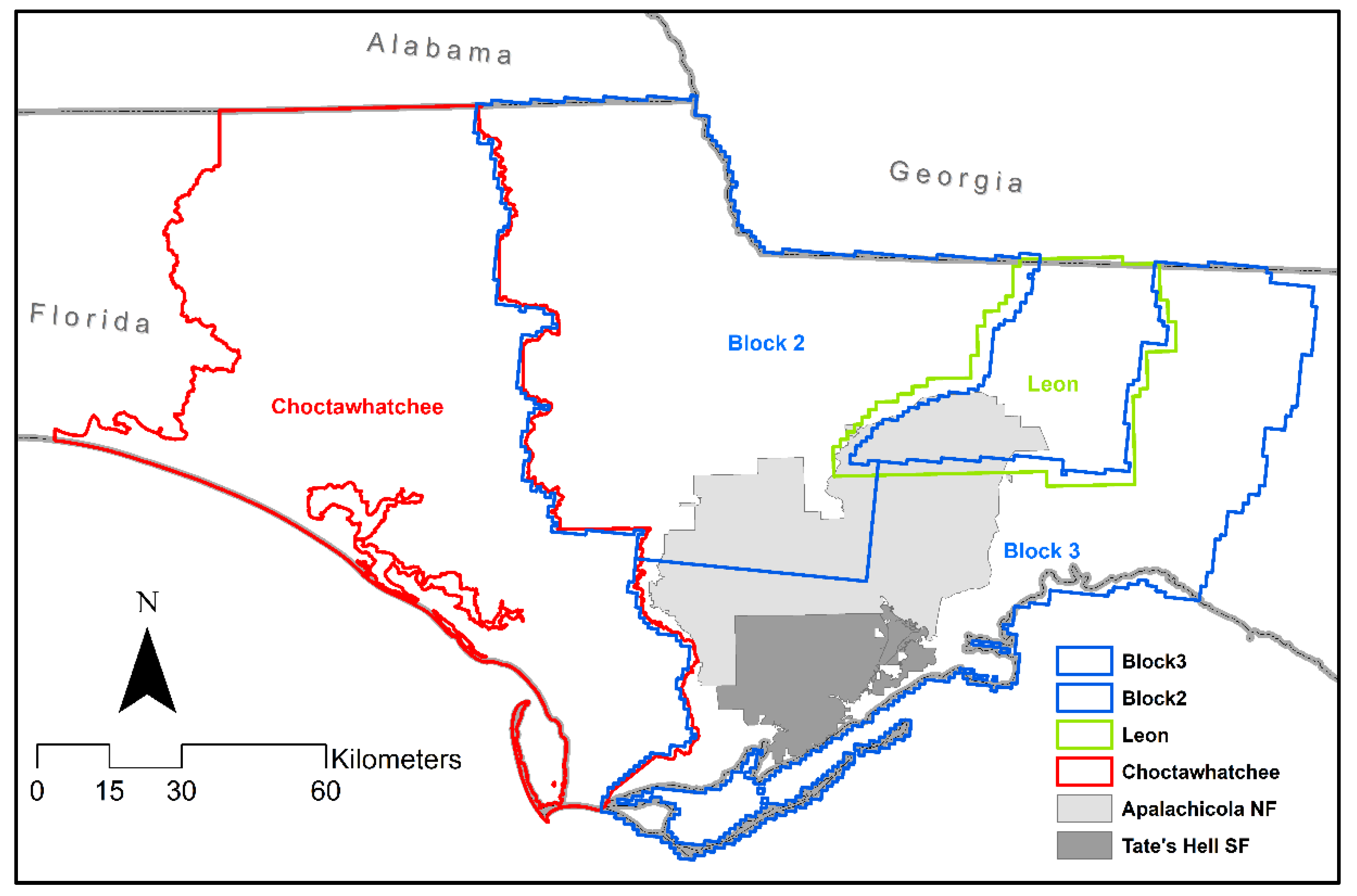
2.1. Study Area

The area of interest in this study consisted of 11 contiguous counties in the Florida Panhandle totaling about 22,900 km2. This area contains various publicly held lands, including the Apalachicola National Forest and Tate’s Hell State Forest (Figure 1). Forested lands, both public and private, are a key component to this area’s status as a North American biodiversity hotspot [23]. This area is also the focus of multiagency long-term restoration projects [24] related to the presence of the threatened longleaf pine ecosystem [25] and the downstream Apalachicola Bay, which was impacted by the Deepwater Horizon oil spill [26]. This area was also heavily impacted by category 5 Hurricane Michael on 7 October 2018; however, all the data presented here were collected prior to Michael’s landfall.

2.2. Forestry Plot Data

The 246 forested field plots used in this study were established between December 2017 and March 2018. These plots were designed to be related to remotely sensed data following recommendations from Hogland et al., 2020 [27]. The plots were 36 m square plots containing four 9 m diameter nonoverlapping subplots. The area of the subplots, where observations were taken, represented 78.5% of the total area of the plot. Subplot observation data consisted of tree species, tree condition, and diameter at breast height (DBH) for each tree within the subplots, as well as vegetation cover for the entire subplot and subplot tree counts. These plots covered 27 unique natural communities as defined by the Florida Natural Areas Inventory [28], of which the most common were pine plantations, wet and mesic flatwoods, and sandhills.
Forest structural metrics produced in this study were trees per hectare (TPH), basal area, and quadratic mean diameter (QMD) for living trees. TPH was the number of tree stems in a hectare area; basal area was the cross-sectional area of trees at breast height with the units of meters squared per hectare (m2/ha). Within each subplot, individual tree’s DBH were measured in square inches; this measurement was used to calculate the basal area in square feet using Equation (1):
BA = 0.005454 × DBH2
The basal area for each tree was converted to square meters and then summed to the subplots; an expansion factor of 9.8 was used to convert from square meters per subplot to meters square per hectare. QMD is a commonly used measure of central tendency in forestry, and was calculated using (Equation (2)):
QMD = D i 2 n
where Di is the diameter at breast height in centimeters of the ith tree and n is the number of trees in the plot. Summary statistics from our forested field plots are shown in Table 1.

2.3. Lidar Data

Lidar data for this study were obtained from the United States Geological Survey 3D Elevation (3DEP) Program [2]. Lidar was delivered as four collections of classified LAS version 1.4 files. We refer to these collections as Leon, Block 2, Block 3, and Choctawhatchee (Figure 1). The Leon lidar collection consisted of 876 (5000 ft × 5000 ft) tiles covering all of Leon County. Leon data had a nominal pulse spacing (NPS) of 0.35 m and was acquired between 5 February 2018 and 25 April 2018 [29]. Blocks 2 and 3 consisted of 6845 and 6598 (1 km × 1 km) tiles, respectively, and covered the western and southern counties surrounding Leon County (Figure 1). Block 2 and Block 3 lidar were collected in early 2018 and had an NPS of 0.7 m [30]. The Choctawhatchee data were acquired in early 2017, and had an NPS of 0.7 m. The Choctawhatchee lidar collection consisted of 3893 (1 km × 1 km) tiles [31].

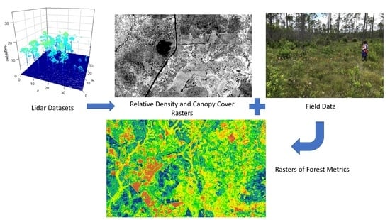
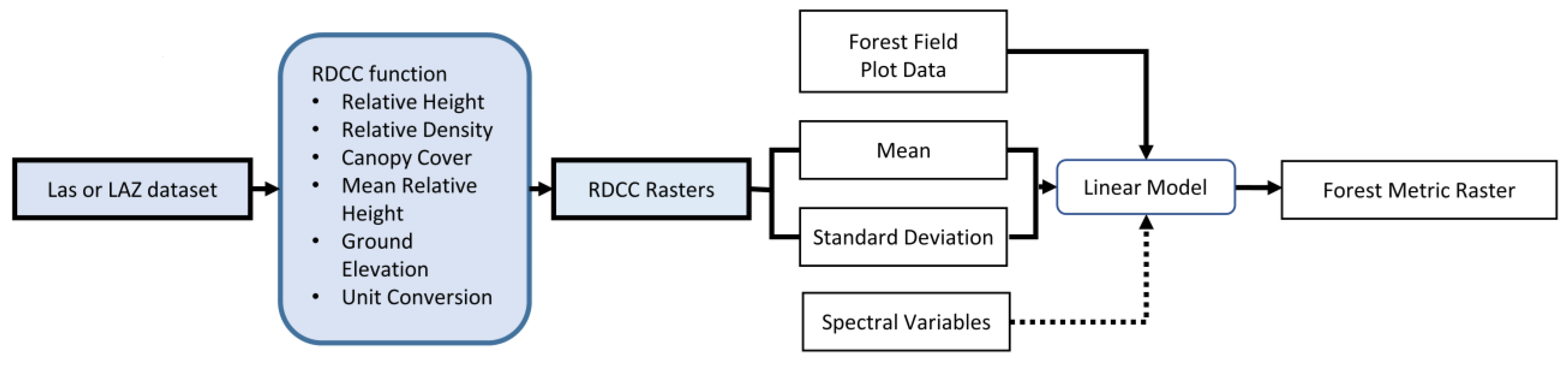
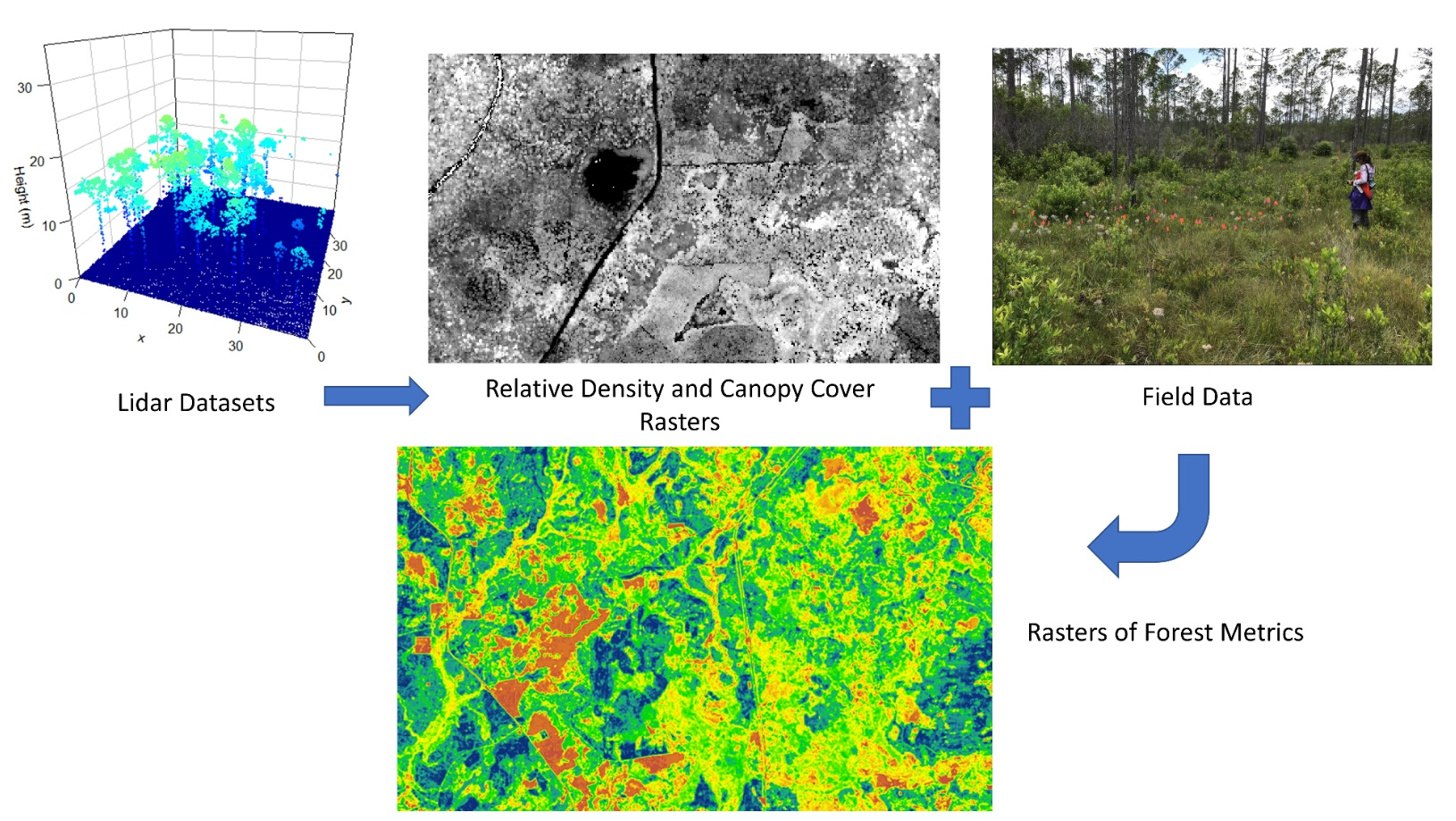
2.4. Relative Density Canopy Cover Function

Analysis was conducted using the R statistical software [32], and the R package lidR (version 3.1.2) [22,33]. This software package is free, open source, and available for multiple operating systems. In addition, lidR is readily customizable and provides many advanced functions for working with lidar data for forestry applications. For correlation analysis and figure production, the following R packages were utilized: PerformanceAnalytics [34], corrplot [35], and Hmisc [36].
The relative density canopy cover function (RDCC) is a custom forest metric function we built using tools provided in the lidR package [22,33]. This function provided specific forest metric outputs (Table 2) identified as useful for quantifying tree volume, density, and canopy cover in previous work [5,11]. Additionally, cover and density metrics specific to multiple forest canopy layers (shrub, low midstory, high midstory, and upper canopy) were produced using the RDCC function, as these have been identified as important for multiple forest management objectives [8,11,12].
We applied the RDCC function to our four lidar datasets in R version 4.0.1 using lidR’s “LAScatalog processing engine” [33], which is a tool to manage large numbers of lidar point cloud files. LidR’s LAScatalog processing engine handles buffering, merging, and parallel processing required to efficiently process large LAS collections [33]. The RDCC function also includes vertical and horizontal unit checks of the LAS data, and automatically converts units to meters from feet, as was the case for Leon County and Choctawhatchee LAS files. The adjustable output raster horizontal grid cell size was set to 5 m. The RDCC function’s multiband TIF raster output was reprojected to UTM Zone 16N using a separate R function.
The RDCC function took LAS or LAZ file inputs and outputted 2D multiband raster .tiff files containing 28 variable bands (Table 2) at a user-defined cell size. The first four variable band outputs from the RDCC function were general point cloud summary metrics useful for QA/QC and the generation of the proceeding 24 variable bands. Band 1 was the total number of returns in a cell, and was used as the denominator in the relative density variable bands. Band 3 was the number of first returns in a cell, and was used in the canopy cover calculations. Band 2 was the number of ground returns, and band 4 was the ground elevation. These bands defined ground points in one of two ways. If point clouds were classified following the American Society for Photogrammetry and Remote Sensing LAS classification format 1.4 (or previous versions) [37], RDCC defined ground points as any points of code 2 (ground), 7 (low points), 9 (water), or 11 (road surface). If there was at least one ground point in a cell, the ground elevation (variable band 4) was defined as the mean elevation of ground points. If there were no classified ground points within a cell, then ground elevation was defined as the mean elevation of the lower 5% of all points. Ground elevation was then used to normalize the height of remaining cell points (i.e., height above ground) to derive the canopy metrics shown in Table 2.
This memory-resident method of normalizing point clouds is atypical, but was used in this study to address several issues that arose when processing large LAS datasets. The first issue with normalizing point cloud data using traditional LAS functions, even those included in the lidR package, is that they roughly double the size of LAS datasets by writing new normalized LAS files to disk. This process would have increased data storage requirements from ~10.7 TB to ~21 TB, and significantly increased processing time. In addition, processing time can be compounded due to error handling in edge cases. This method avoided those issues; however, ground point and normalization routines currently used in the RDCC function should only be deployed with fine spatial resolution cell sizes and in areas without significant topography. This study area did not have severe topographical changes, as can be seen in Table 1. When LAS file height normalization was run prior to processing the RDCC function had to be modified to account for this prior normalization. The R code for the RDCC function is provided in Appendix A.
RDCC output bands 5 and 6 provided means and standard deviations, respectively, for all relative heights within the cell. Bands 7 through 13 were the relative height bands at set height percentile increments. Relative height was the height above ground elevation at which the indicated percentage of returns was reached. Bands 14 to 28 used set height breaks that were meant to reflect the canopy layers of interest in the study area based off [11]. These layers were the shrub layer at a 0.6096 m to 3.048 m height, the high shrub or low midstory layer at 3.048 m to 6.096 m, the high midstory layer of 6.096 m to 14.935 m, and the upper canopy layer with returns greater than 14.935 m. Bands 14 to 16 were relative density within the shrub, low, and high midstory layers. Bands 17 to 20 were relative density greater than the lower range of each canopy height break and lower than the upper range of each canopy height break. The equation for relative density is shown as Equation (3):
R D = a ϵ r e t u r n s [ L H a < U H ] a ϵ r e t u r n s [ a ]
where RD is relative density, a is all returns in a cell, LH is the lower height break, and UH is the upper height break. Bands 21 to 24 were canopy cover greater than the lower range of each canopy height break and lower than the upper range of each canopy height break. The equation for canopy cover is shown as Equation (4):
C C = f ϵ r e t u r n s [ L H f < U H ] f ϵ r e t u r n s [ f ]
where CC is canopy cover, f is first returns in a cell, LH is the lower height break, and UH is the upper height break. The final four bands, 25 to 28, were the mean of all relative heights greater than the lower range of each of the four canopy height breaks.

2.5. Cloud Processing

This study used a Microsoft Azure cloud computing environment for data processing as part of an AI for Earth grant. A Linux virtual machine running Ubuntu server 20.04 LTS with 32 GB RAM was deployed in our Azure cloud environment and loaded with R Studio software (version 1.4) package. Our custom lidR function RDCC was run in parallel on this virtual machine using 30 logical cores. Four lidar datasets, totaling 18,212 LAS files and ~10.77 terabytes (TB), were processed separately. The lidar data, as LAS 1.4 files, were stored in blob storage in our Azure environment and were accessed from our Linux virtual machine; raster outputs were also saved back to this blob storage container, and links to these output folders were shared directly with project partners.

2.6. Forest Metric Models and Raster Outputs
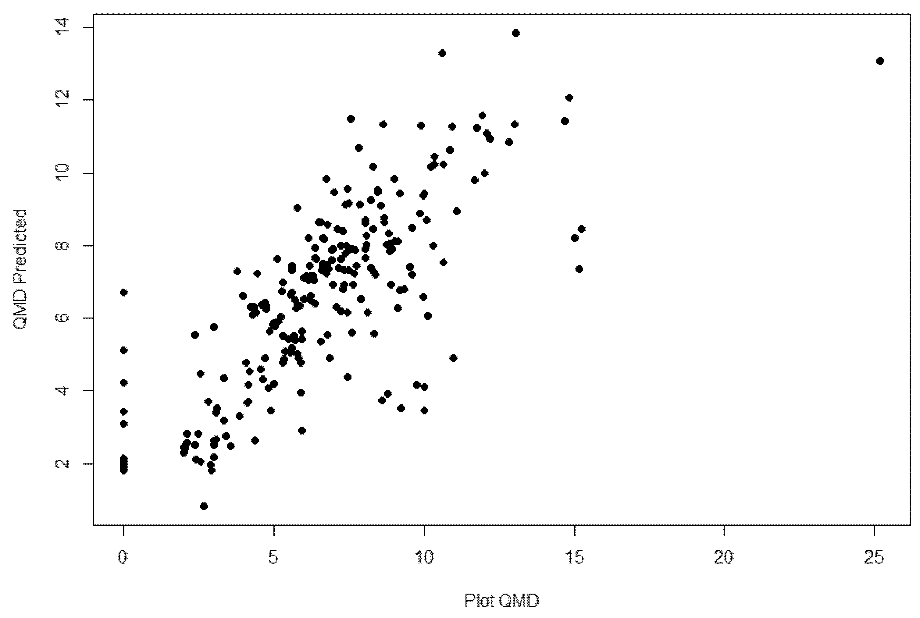
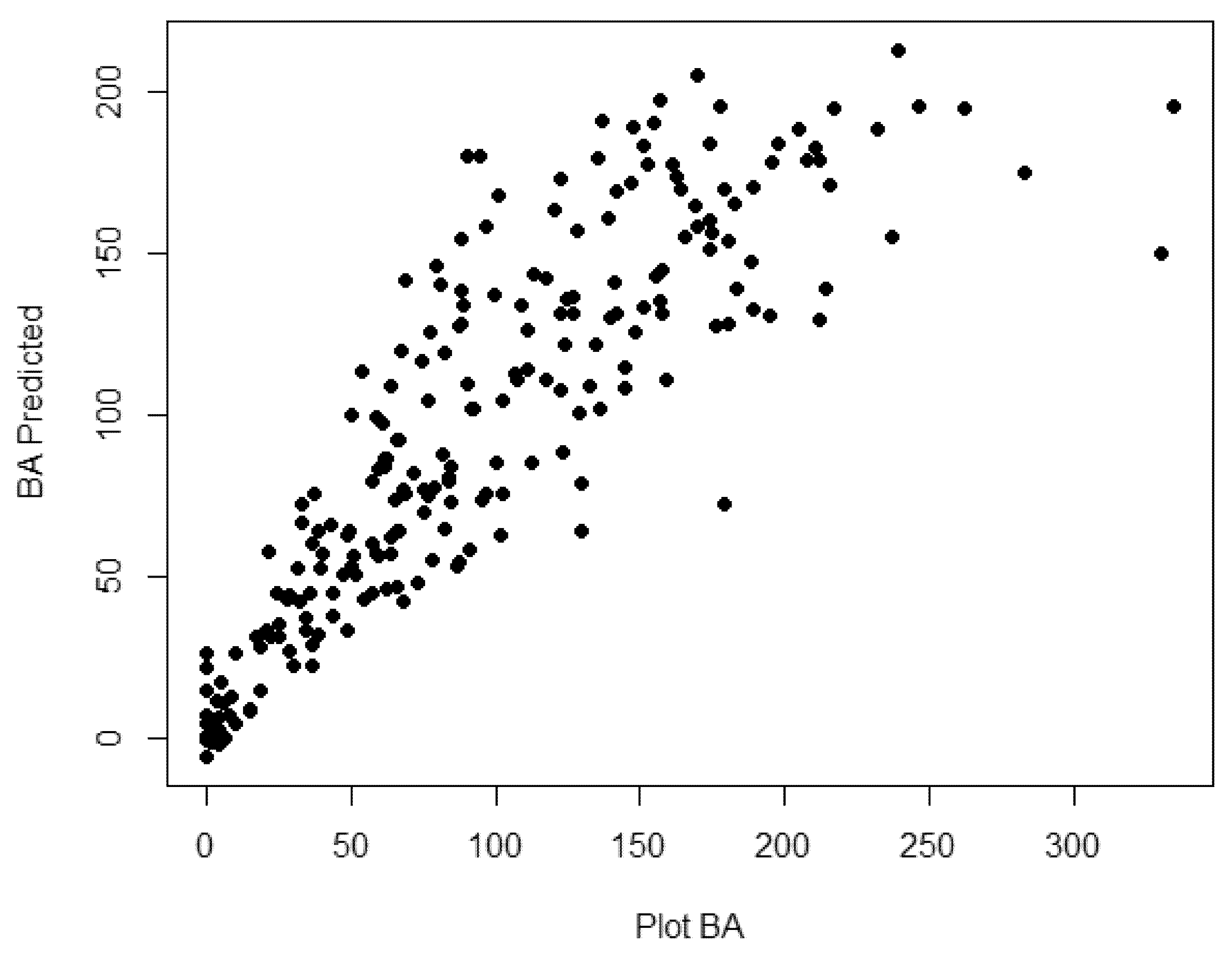
Model development and raster analysis were performed using R statistical software (R Core Team, 2021), ESRI geographic information system (ArcGIS), and the ArcGIS plug-in RMRS Raster Utility toolbar [38]. RDCC output rasters of lidar data were transformed into predictive rasters with 5 m cell resolution, which represented the values at that point as if it was the center of a 40 m × 40 m forest plot. This was done using the tools provided in the RMRS Raster Utility toolbar, specifically the ‘Extract Bands’, ‘Focal Analysis’ using the mean and standard deviation and an 8 × 8 multiplier, and ‘Create Composite’ tools [38]. These tools calculated the plot-level mean and standard deviation of bands 5 through 24 of the RDCC outputs, a total of 40 variables, across the study area. The cell values of this 40-band raster were extracted at the forest plot locations, using the ‘Sample Values’ tool found in the RMRS Raster Utility toolbar [38]. These values were appended to the forest plot summary tables that were subsequently used in the R statistical software for model development.
Predictor variables were selected from the 40 available variables to create general linear models of BAH, TPH, and QMD following the R script sequential general additive model (GAM) routine detailed in Hogland et al., 2019 [39], using the gaussian family and identity link distribution, alpha of 1, and increases in percent deviance threshold set to 0.005. These conservative thresholds, especially the alpha value, were set to allow for the least number of variables to be removed from the model at this step. The second variable selection step was to create a general linear model using all the variables selected in the first step and then to manually perform a reverse stepwise selection using the significance of each variable. This step was used to remove non-significant variables while maximizing the models’ overall adjusted r2 value. Once this step was complete, further variable selection was performed by comparing models with different variables using their Akaike information criterion (AIC) [40], root mean square error (RMSE), and mean absolute error (MAE) scores, with the emphasis on selecting the most parsimonious model for each forest metric.
For the imagery-only models and the combined imagery and lidar models, we used pre-Hurricane Michael Sentinel-2 data from previous work in this study area [41]. This imagery data consisted of the blue, green, red, and near-infrared spectral bands with a spatial resolution of 10 m, and was a combination of images taken in two phenological time periods, winter and spring, with individual scene acquisition dates in 2017 and 2018. Sentinel-2-only models of BAH that were presented in [41] were used directly for comparison here, while Sentinel-2 models of TPH and QMD were created in R using the spectral data values of our field plots from the same study. These models had variables designated following the same forward stepwise GAM selection, and backwards manual selection processes as the RDCC (lidar-only) models, the exception being that combination models required at least one predictor variable from both lidar and Sentinel-2 imagery-derived data. Figure 2 displays our general workflow.

3. Results

The RDCC function output resulted in a multiband raster dataset of 18,212 ~1 km × 1 km files (1524 m × 1524 m for Leon) of 5 m spatial-resolution-summarized lidar variables. This process took 28.5 h to complete for the entire ~22,900 km2 study area. These multiband rasters provided useful outputs without further processing. However, a linear artifact was noted in the raster outputs from Blocks 2 and 3 in the 50% percentile relative height band and shrub relative density bands. This linear gap of no data correlated to the edge of flight lines and was generally as wide as the raster’s 5 m cell size, but extended over the edge of the entire flight line. We determined that this midstory gap was due to an extreme scan angle at the scan overlap juncture. We attempted to fix this artifact by using all points, and not excluding the points categorized as withheld by the original contractor and using the scan angle of the returns to individually exclude points in the point cloud by their scan angle. By doing this, we were able to remove the linear gaps in our rasters; however, this also created different artifacts in our other RDCC bands, and therefore this method was not used.
Combined models and lidar-only models showed very similar results (Table 3), while the Sentinel-2 imagery-only models had the highest measure of errors and lowest adjusted r2 across all response variables when compared with the models that used lidar data. Combination models had the highest adjusted r2 values and lowest AIC scores, except for the TPH models and the MAE for QMD models, where the RDCC models performed slightly better. The Sentinel-2 basal area model used here varied slightly from the one presented in [41], as that study used a hurdle modeling approach to exclude field plots with zero basal area (n = 2), while this study included the zero basal area plots.
The full list of the variables selected for use in these general linear models is shown in Appendix B. The most selected variable was the relative density 3.048 m to 6.096 m variable (RD_10to20ft), followed by the canopy cover greater than 3.048 m variable (CC_gt10ft). RD_10to20ft was selected in every single model when it was available, while the CC_gt10ft was selected in all the RDCC and combo BAH and TPH models. These two variables were moderately correlated, but still provided complimentary information about the forest structure. The correlation chart of the four variables used in the BAH RDCC model is presented in Figure 3, and shows the variables’ distribution in the diagonal boxes, as well as their bivariate correlation scatterplots, correlation scores, and significance.
As seen in Figure 3, RD_10to20ft was only slightly correlated with one of the other two variables selected in the model besides CC_gt10ft, while CC_gt10ft was strongly correlated with both. The correlation plot of the BAH combo model, which included the Sentinel-2-derived PCA variables and is shown in Figure 4, demonstrates that the RD_10to20ft variable was also not significantly correlated with the Sentinel-2 variables selected in that model. This pattern continued across all models and variables (see Figure A1, Figure A2, Figure A3, Figure A4, Figure A5 and Figure A6), suggesting that RD_10to20ft was capturing unique information about forest structure that other variables were not, including the Sentinel-2 imagery-derived variables. CC_gt10ft contained much of the same information that the other variables provided, leading to these two combined variables capturing much of the information provided in all RDCC variables as they related to basal area, trees per area, and quadratic mean diameter.
Using the RMRS Raster Utility Arc plugin [38], the RDCC models from Table 3 (also see Figure A7, Figure A8 and Figure A9) were used to produce raster surface outputs of BAH, TPH, and QMD. These raster outputs were shared with forestry professionals in the study area to assess their practical and qualitative value, and were given a positive assessment. Sharing was facilitated by providing weblinks to cloud-stored raster data given to practitioners. Figure 5 shows the BAH raster that was produced from our RDCC model and distributed over the entire ~22,900 km2 study area.

4. Discussion

In this study, we used the lidR R package and our lidR user-extension function, referred to as RDCC (Appendix A), to rapidly process a very large (~11 TB) lidar point cloud dataset into multiband rasters of height, relative density, and canopy cover forest structure metrics. This process was relatively user friendly; and used free, open-source, and scalable software, lowering the barriers for using lidar data at regional scales. It was also a robust and transferable process that worked with lidar datasets with different units, without classified ground points, and even from different lidar platforms. This transferability allowed us to rapidly create products for forest managers without first needing to classify the point cloud, which could be very important in time-sensitive scenarios such as during postdisaster forest-damage assessments.
The free, open-source, and scalable design allows this workflow to be used on local computers, a hybrid cloud computing environment, or a fully cloud-based environment using any modern operating system. We chose to use a distributed cloud computing environment because of the advantages such a setup could provide, specifically scalability and processing efficiency [42]. The lidR package’s parallel-processing capabilities allowed this workflow to be easily scalable [33]. Scalability in the cloud environment refers to the ability to easily increase the number of our virtual machine’s logical cores, the number of virtual machines, and increases in data storage without ever having to buy or maintain hardware [42]. For example, by reading lidar point cloud data directly from a blob storage container (and writing raster products back to this container), we were able to reduce storage costs compared to adding large, high-speed solid-state drives, and still gained the processing benefit of collocating our data with computational resources. However, we did not have to rely heavily on the scalability of the cloud environment to process our data efficiently. The R studio, lidR software package, and our RDCC function were efficient enough at processing large lidar datasets that we did not encounter a processing bottleneck when using our moderately equipped VM, which had the processing power equivalent to our physical workstations. To process much larger extents, or much higher density lidar datasets, such as state or regional scale projects, additional scaling of the cloud environment would be required for timely processing.
As a general comparison, this study processed lidar data covering 22,900 km2 into 28 band 5 m cell GeoTIFFs in 28.5 h, while the equivalent processing software ‘Laserchicken’ reported processing a 30,000 km2 lidar dataset into 22-band, 10 m cell GeoTIFFs over 96 h [3]. This is not a direct comparison, as ‘Laserchicken’ calculates several process-intensive lidar features, such as eigenvalues, that our RDCC function does not. However, it demonstrated that this workflow performed well compared to other lidar-processing studies.
Our forest metric model results also compared favorably with previous studies. For example, Sousa da Silva et al., 2019 modeled basal area in Eucalyptus plantations with r2 values ranging from 0.67 to 0.81 [43]; Pearse et al., 2018’s basal area model had an r2 value of 0.58 [6]; and Woods et al., 2008 had r2 values of basal area of 0.79 to 0.85 and QMD of 0.68 to 0.83 [44]; and van Ewijk et al., 2011 had QMD r2 = 0.68. However, van Ewijk et al., 2011 used field data in combination with lidar data to estimate QMD, and not just to train their model [45]. Ahl et al., 2019 used random forest (RF) to model basal area and QMD from lidar, with RMSEs of 9.0 and 11.7, respectively [9]. These studies had higher lidar point densities and covered smaller study areas with a smaller range of forest types than our study, yet our best model results for BAH and QMD had similar or better r2 and RMSE values (adj. r2 = 0.80, adj. r2 = 0.58; and RMSE = 7.59, RMSE = 5.428, respectively).
In this study, we showed that lidar-derived canopy metrics produced better models of forest structure when compared with Sentinel-2-only models, though this is not always that case, as [9] demonstrated. Additionally, when we combined imagery and lidar variables in our forest metric models, we created marginally better estimates for two out of our three forest metrics. However, our model comparison results were possibly influenced more by spatial resolution then data type, as the Sentinel-2 imagery data had a 10 m cell size, meaning only 16 cells were within each field plot. The lidar-data-derived raster’s cell size was 5 m, allowing for 64 cells for each field plot, and therefore contained more textural information. Our correlation matrix of variables (Figure 3 and Figure 4) did show that the lidar data contained important midstory variables that the spectral imagery alone did not. The degree of difference in our model results due to spatial resolution and observations between lidar and spectral imagery is yet to be determined.
We chose to use easily interpretable general linear models for our forest metric models. General additive models (GAMs) were also explored to create the BAH, TPH, and QMD model estimates, but were not found to add significant predictive power over the general linear models. The interpretability of general linear models, over more ‘black box’ models such as RF, allowed us to easily identify the selection of the low midstory relative-density variable in all RDCC and combination forest metric models, and some studies have found that linear models outperformed RF when modeling forest metrics from lidar data [43]. Our variable correlation results (Figure 3, Figure 4, Figure A1, Figure A2, Figure A3, Figure A4, Figure A5 and Figure A6) indicated that the relative density of low midstory was a variable that captured unique data in our study area that was important for estimating several forest metrics. We are not aware of any other studies that have shown the importance of a lidar-derived midstory metric for estimating a broader forestry metric such as BAH, TPH, or QMD. We also discovered a linear artifact in some datasets that affected points at the edges of flight lines related to this important low midstory metric. This was the result of high scan angles at the flight line overlaps. High scan angles were shown to impact forest metrics estimates in at least one other study [46]. Future airborne lidar contracts should address this issue by incorporating stricter limits on allowable scan angles, which will help avoid gaps in the midstory canopy at flight line overlaps.
This study focused on estimating forest metrics using an area-based approach. A potential next step would be to develop similar workflows focused on individual tree observations from high-resolution point clouds that currently face the same processing bottleneck that we addressed in this study. Previous studies have already shown the value of lidar data from drone platforms, such as Dalla Corte et al., 2020, who estimated tree diameter and height from drone-based lidar using R software packages [47]. Processing these individual tree metrics from lidar datasets is becoming more accessible using free and open-source R software packages [48]. To process large-extent lidar datasets using an individual tree approach efficiently will require the creation of workflows such as that presented in this study.

5. Conclusions

While lidar data is increasingly available, analysis of lidar data for forest structure is not yet ubiquitous. This can lead to natural resource managers being data rich, but information poor. In this study, we presented a practical, scalable, and free workflow to help derive useful information from large lidar datasets. We used free, open-source, and user-extendable software in a cloud-based environment to efficiently process ~11 TB of lidar point cloud data covering 22,900 km2 of a diverse landscape containing at least 27 natural communities. Our lidar processing workflow outputted 28-band, 5 m cell spatial resolution height normalized GeoTIFFs, containing relative height, relative density, and canopy cover data. These outputs were used to develop general linear models of BAH, TPH, and QMD, which outperformed Sentinel-2 imagery-based models in our study area, and performed as well or better than previous studies using higher-density point clouds in much smaller, less structurally diverse landscapes. This ability to quickly process landscape scale lidar data, with user-created functions, into forest metrics has only recently been possible, as analysis software such as the lidR [22] package have become available. We overcame the processing bottlenecks that large lidar datasets present by using software designed for parallel processing (lidR) coupled with a distributed cloud computing environment. In creating our models of BAH, TPH, and QMD, we discovered the importance of our relative density of low midstory lidar variable (RD_10to20ft). This variable was shown to contain information that was not captured in other lidar and Sentinel-2 variables.
Having refined and readily available workflows that extract forest metrics from lidar data, similar to the standardization of DEM production from lidar, that overcome big data processing bottlenecks will provide land managers, researchers, and the general public with valuable information about landscapes at fine spatial resolutions. This will allow for precise, efficient, and relatively inexpensive habitat and ecosystem monitoring, as well as rapid disaster response and mitigation, and prescribed fire management. Future work can also be done to extend these workflows to include and be integrated with individual tree metrics from drones or terrestrial-based lidar systems, which may further improve the information for landscape-level monitoring and management.

Author Contributions

Conceptualization, J.S.P., J.D., and P.M.; methodology, J.S.P., and J.D.; software, J.D., and J.S.P.; validation, P.M., J.D., and J.S.P.; formal analysis, J.S.P.; investigation, J.S.P.; resources, V.I., P.M., and J.D.; writing—original draft preparation, J.S.P.; writing—review and editing, J.D., P.M., and V.I.; visualization, J.S.P.; supervision, V.I., J.D., and P.M.; project administration, J.D., P.M., and V.I.; funding acquisition, V.I., J.D., and P.M. All authors have read and agreed to the published version of the manuscript.

Funding

This research was funded by the Gulf Coast Ecosystem Restoration Council (RESTORE Council) through an interagency agreement with the USDA Forest Service (17-IA-11083150-001) for the Apalachicola Tate’s Hell Strategy 1 project; as well as a subscript grant for Microsoft AI for Earth (CSER AI for Earth Sponsorship).

Acknowledgments

We thank Marck Vaisman for supporting our cloud infrastructure and Jordan Vernon for her editorial and technical advice.

Conflicts of Interest

The authors declare no conflict of interest. The funders had no role in the design of the study; in the collection, analyses, or interpretation of data; in the writing of the manuscript; or in the decision to publish the results.

Appendix A

The following is the custom code used within the lidR R package to process the lidar data in this study. It includes three functions: two to check and adjust the vertical and horizontal units to meters if they are in feet, and the metrics custom function that created the RDCC outputs discussed in this study and used the lidR tools. Finally, this code contains lines demonstrating how to call these functions in R.
## Example LAS files can be obtained at: https://apps.nationalmap.gov/downloader/#/ (accessed on 18 November 2021) in the data section check the Elevation
## Source Data (3DEP)—Lidar, lfSAR box and the lidar point cloud box. Use the viewer to navigate to your location of interest
## search products then click on download link (LAZ) next to the las files you are interested in, use 2 or more las or laz files
## and place in the same folder so that you can create a las catalog for use with this script, bulk download options are also
## available on the site.
## For lidR help, tutorials and updates visit https://github.com/r-lidar/lidR/wiki (accessed on 18 November 2021)
## Install/Load packages
if (!require(“pacman”)) install.packages(“pacman”)
pacman::p_load(pacman, tidyverse, progress, rgdal, lidR, sf, raster, stringr, future)
 
## This function checks OS and converts file paths to comply
get.paths <- function(paths)
{
 file_names <- strsplit(paths, “;”)[[1]]
 if (Sys.info()[[“sysname”]] != “Windows”)
 {
    file_names <- gsub(‘\\\\’, ‘/’, file_names)
    file_names <- gsub(‘C:/Users/’, ‘/mnt/windows_data/’, file_names)
 }
 file_names
}
# Function to get name of first file in folder, default suffix set to ‘las’, for .lax files provide “laz” for suffix when calling function
firstPath <- function(folder, suffix = “las”){
 file_ls<-list.files(folder, pattern=paste0(‘\\.’, suffix))
 first_las<-get.paths(paste0(folder,“\\”,file_ls[1]))
}
# Function to check if the vertical units are in feet
vertFTcheck <- function(las_file_path){
 las = suppressWarnings(readLAS(las_file_path))
 string_test = wkt(las)
 ht_loc<-stringr::str_locate(string_test, fixed(“height”, ignore_case = TRUE))
 if (is.na(ht_loc[2])){
    ft = FALSE
 } else {
    sub_ht<- substr(string_test, ht_loc[2], ht_loc[2] + 25)
    ft<-str_detect(sub_ht, “ft|feet|FT|Feet”)
 }
 las = NULL
 return(ft)
}
# Function to check if the horizontal units are in feet
horFTcheck <- function(las_file_path){
 library(stringr)
 las = suppressWarnings(readLAS(las_file_path))
 string_test = wkt(las)
 if(string_test == ”){
    print(“Empty wkt file, no hor unit check done”)
 }
 else{
    ## now search the wkt for the northing keyword ignoring case
    hor_loc<-str_locate(string_test, fixed(“false_northing”, ignore_case = TRUE))
    sub_hor<- substr(string_test, hor_loc[2]+10, hor_loc[2] + 35)
    ft_hor<-str_detect(sub_hor, “foot|Foot|ft|FT|Feet|feet”)
    las = NULL
    return(ft_hor)
 }
}
rdcc_metrics <- function(z, Classification, RetNum, folder, ft_yes = FALSE) {
 n = length(z) #Total number of returns in cell
 zq = stats::quantile(z, probs = seq(0.05, 0.95, 0.05)) #Quantiles of all elevations within cell
 zqnum <- as.numeric(zq) #Removing names from quantile output, just array of numeric values
 grndpts<- z[Classification==2 | Classification==7 |Classification==9 | Classification==11]
 ngrndpts =length(grndpts)
 if (ngrndpts >= 1)
 {
    grndelev <- mean(grndpts) #Calc mean elevation of ground return pts
    zqnumrel = zqnum - grndelev #Normalize all quantile elevations to be relative above ground level
    zrel = z -grndelev #Normalize ALL return elevations to be to be relative above ground level
 }
 else
 {
    grndelev <- zqnum[1] #use 5% elev as a proxy ground elevation
    zqnumrel = (zqnum - grndelev) #Normalize all quantile elevations to be relative above ground level
    zrel = z -grndelev #Normalize ALL return elevations to be to be relative above ground level
 }
 ## now use result of ft_yes to adjust heights to meter
 if (ft_yes==TRUE){
   grndelev <- grndelev/3.28084
   zqnumrel <- zqnumrel/3.28084
   zrel <- zrel/3.28084
 }
 ht_breaks<-c(0.6096,3.048,6.096,14.9352)
 zrelmax <- max(zrel)
 #Now create a RasterBrick of all outputs
 list(
    nreturns <- n,
    ngrndreturns <- ngrndpts,
    nfirstreturns <- length(zrel[RetNum==1]),
    grndelev,
    MnRH <- mean(zrel),
    SDRH <- stats::sd(zrel),
    RH95 <- zqnumrel[19],
    RH90 <- zqnumrel[18],
    RH75 <- zqnumrel[15],
    RH50 <- zqnumrel[10],
    RH25 <- zqnumrel[5],
    RH10 <- zqnumrel[2],
    RH05 <- zqnumrel[1],
    RD2to10ft <- length(zrel[zrel<ht_breaks[2] & zrel >=ht_breaks[1]])/n,
    RD10to20ft <- length(zrel[zrel<ht_breaks[3] & zrel >=ht_breaks[2]])/n,
    RD20to49ft <- length(zrel[zrel<ht_breaks[4] & zrel >=ht_breaks[3]])/n,
    RDgt2ft <- length(zrel[zrel>=ht_breaks[1]])/n,
    RDgt10ft <- length(zrel[zrel>=ht_breaks[2]])/n,
    RDgt20ft <- length(zrel[zrel>=ht_breaks[3]])/n,
    RDgt49ft <- length(zrel[zrel >=ht_breaks[4]])/n,
    CCgt2ft <- length(zrel[zrel >=ht_breaks[1] & RetNum==1])/length(zrel[RetNum==1]),
    CCgt10ft <- length(zrel[zrel >=ht_breaks[2] & RetNum==1])/length(zrel[RetNum==1]),
    CCgt20ft <- length(zrel[zrel >=ht_breaks[3] & RetNum==1])/length(zrel[RetNum==1]),
    CCgt49ft <- length(zrel[zrel >=ht_breaks[4] & RetNum==1])/length(zrel[RetNum==1]),
    if (zrelmax > ht_breaks[1]) {MnRHgt2ft <- mean(zrel[zrel >=ht_breaks[1]])} else {MnRHgt2ft <- numeric(0)},
    if (zrelmax > ht_breaks[2]) {MnRHgt10ft <- mean(zrel[zrel >=ht_breaks[2]])} else {MnRHgt10ft <- numeric(0)},
    if (zrelmax > ht_breaks[3]) {MnRHgt20ft <- mean(zrel[zrel >=ht_breaks[3]])} else {MnRHgt20ft <- numeric(0)},
    if (zrelmax > ht_breaks[4]) {MnRHgt49ft <- mean(zrel[zrel >=ht_breaks[4]])} else {MnRHgt49ft <- numeric(0)}
    )
}
## User Input for folder of las files
folder<- readline(prompt = “Enter las directory path: ”)
out_dir<- readline(prompt = “Enter output directory path: ”)
user_out_suffix <- readline(prompt = “Enter output tif file suffix for example Block1: ”)
out_suffix <- gsub(“ ”, “”, gsub(“/”,“”, user_out_suffix))
user_cell_size <- as.numeric(readline(prompt = “Enter output cell size in meters: ”))
## Creating a LAScatalog, filter values are only suggestions please use filters that are appropriate for your data
ctg = readLAScatalog(folder, progress = TRUE, filter=“-drop_withheld -drop_class 18 -drop_z_below -5”)
opt_select(ctg) <- “xyzciReturnNumber”
## make output file name
opt_output_files(ctg)<-get.paths(paste0(out_dir, “\\”, out_suffix, “_{ORIGINALFILENAME}”))
## Deciding whether ft or meter for horizontal, relies on keywords in first las file’s wkt
first_las<-firstPath(folder)
ft_hor <- horFTcheck(first_las)
if (ft_hor==TRUE){
 cell_size<-user_cell_size*3.28084
} else {
 cell_size<-user_cell_size
}
## ft_yes function deciding whether ft or meter for vertical using first las file in folder
ft_yes = vertFTcheck(first_las)
##Parallel computation, number of workers is how many las files in the catalog will be processed, set lidr threads is the
##number of cores working on each file at a time. future::availableCores() uses the future package to automatically select
## the number of available cores, this number is then divided by two which is the number used in set lidr threads and
##subtracted by one so some logical cores are available for work outside this function. All these settings can be changed
##manually these are just defaults
plan(multisession, workers = (future::availableCores()/2)-1)
set_lidr_threads(2L)
## Running the rdcc function – named ‘rdcc_metrics’
RDCCmetrics <- grid_metrics(ctg, ~rdcc_metrics(z=Z, Classification = Classification, RetNum = ReturnNumber, folder=folder, ft_yes = ft_yes), cell_size)

Appendix B

The following is the full list of the predictive variables and their descriptions used in the final general linear models of basal area per hectare, trees per acre, and quadratic mean diameter. For details on production and interpretation of Sentinel-2 principal component analysis (PCA) variables, see St. Peter et al., 2020. Variables beginning with the ‘Sent’ came from Sentinel-2 imagery; all other variables were derived from the Lidar RDCC function described in this paper.
BAH Sentinel-2 Model variables:
Sent_Pred_Band2 = Plot Mean of PCA 2
Sent_Pred_Band5 = Plot Mean of PCA 5
Sent_Pred_Band6 = Plot Mean of PCA 6
Sent_Pred_Band8 = Plot Mean of PCA 8
Sent_Pred_Band18 = Plot Standard Deviation of PCA band 8
BAH RDCC Model variables:
Pred_Band5 = Plot Mean of Relative Height 75%
Pred_Band11 = Plot Mean of Relative Density 10 to 20 ft (High shrub/low midstory)
Pred_Band18 = Plot Mean of Canopy Cover greater than 10 ft (based only on first returns)
Pred_Band20 = Plot Mean of Canopy Cover greater than 49 ft (based only on first returns)
BAH Combo Model variables:
Pred_Band11 = Plot Mean of Relative Density 10 to 20 ft (High shrub/low midstory)
Pred_Band18 = Plot Mean of Canopy Cover greater than 10 ft (based only on first returns)
Sent_Pred_Band4 = Plot Mean of PCA 4
Sent_Pred_Band7 = Plot Mean of PCA 7
TPH Sentinel-2 Model variables:
Sent_Pred_Band2 = Plot Mean of PCA 2
Sent_Pred_Band3 = Plot Mean of PCA 3
Sent_Pred_Band5 = Plot Mean of PCA 5
Sent_Pred_Band6 = Plot Mean of PCA 6
Sent_Pred_Band10 = Plot Mean of PCA band 10
Sent_Pred_Band13 = Plot Standard Deviation of PCA band 3
Sent_Pred_Band19 = Plot Standard Deviation of PCA band 9
TPH RDCC Model variables:
Pred_Band1 = Plot Mean of Mean of all Relative Heights
Pred_Band5 = Plot Mean of Relative Height 75%
Pred_Band6 = Plot Mean of Relative Height 50%
Pred_Band11 = Plot Mean of Relative Density of all returns 10 to 20 ft
Pred_Band18 = Plot Mean of Canopy Cover greater than 10 ft (based only on first returns)
Pred_Band21 = Plot Standard Deviation of Mean of all Relative Height
Pred_Band33 = Plot Standard Deviation of Relative Density all returns greater than 2 ft
TPH Combo Model variables:
Pred_Band6 = Plot Mean of Relative Height 50% (50th percentile height above ground level)
Pred_Band11 = Plot Mean of Relative Density of all returns 10 to 20 ft
Pred_Band18 = Plot Mean of Canopy Cover greater than 10 ft (based only on first returns)
Pred_Band21 = Plot Standard Deviation of Mean of all Relative Height
Pred_Band33 = Plot Standard Deviation of Relative Density all returns greater than 2 ft
Sent_Pred_Band5 = Plot Mean of PCA 5
QMD Sentinel-2 Model variables:
Sent_Pred_Band1 = Plot Mean of PCA 1
Sent_Pred_Band2 = Plot Mean of PCA 2
Sent_Pred_Band3 = Plot Mean of PCA 3
Sent_Pred_Band7 = Plot Mean of PCA 7
Sent_Pred_Band10 = Plot Mean of PCA band 10
QMD RDCC Model variables:
Pred_Band1 =Plot Mean of Mean of all Relative Heights
Pred_Band2 = Plot Mean of Std. Dev of all Relative heights
Pred_Band4 = Plot Mean of Relative Height 90%
Pred_Band11 = Plot Mean of Relative Density 10 to 20 ft
Pred_Band23 = Plot Standard Deviation of Relative Height 95%
QMD Combo Model variables:
Pred_Band2 = Plot Mean of Std. Dev of all Relative heights
Pred_Band11 = Plot Mean of Relative Density 10 to 20 ft
Pred_Band23 = Plot Standard Deviation of Relative Height 95%
Sent_Pred_Band11 = Plot Standard Deviation of PCA band 1
Figure A1. Correlation chart of TPH RDCC model variables. The variable name and distribution are shown in the diagonal boxes. Below the diagonal are the bivariate scatter plots, with fitted lines showing the relationship between the variables in that column and row. Above the diagonal line are boxes showing the bivariate correlation and the significance of that correlation between the variables in the corresponding column and row; the larger the font, the higher the correlation. For significance, the p-values of 0.001, 0.01, 0.05, and 0.1 correspond to the symbols “***”, “**”, “*”, and “.”.
Remotesensing 13 04763 g0a1
Figure A2. Correlation chart of TPH combination model variables. The variable name and distribution are shown in the diagonal boxes. Below the diagonal are the bivariate scatter plots, with fitted lines showing the relationship between the variables in that column and row. Above the diagonal line are boxes showing the bivariate correlation and the significance of that correlation between the variables in the corresponding column and row; the larger the font, the higher the correlation. For significance, the p-values of 0.001, 0.01, 0.05, and 0.1 correspond to the symbols “***”, “**”, “*”, and “.”.
Remotesensing 13 04763 g0a2
Figure A3. Correlation chart of QMD RDCC model variables. The variable name and distribution are shown in the diagonal boxes. Below the diagonal are the bivariate scatter plots, with fitted lines showing the relationship between the variables in that column and row. Above the diagonal line are boxes showing the bivariate correlation and the significance of that correlation between the variables in the corresponding column and row; the larger the font, the higher the correlation. For significance, the p-values of 0.001, 0.01, 0.05, and 0.1 correspond to the symbols “***”, “**”, “*”, and “.”.
Remotesensing 13 04763 g0a3
Figure A4. Correlation chart of QMD combination model variables. The variable name and distribution are shown in the diagonal boxes. Below the diagonal are the bivariate scatter plots, with fitted lines showing the relationship between the variables in that column and row. Above the diagonal line are boxes showing the bivariate correlation and the significance of that correlation between the variables in the corresponding column and row; the larger the font, the higher the correlation. For significance, the p-values of 0.001, 0.01, 0.05, and 0.1 correspond to the symbols “***”, “**”, “*”, and “.”.
Remotesensing 13 04763 g0a4
Figure A5. Correlation chart of BAH combination model variables. The variable name and distribution are shown in the diagonal boxes. Below the diagonal are the bivariate scatter plots, with fitted lines showing the relationship between the variables in that column and row. Above the diagonal line are boxes showing the bivariate correlation and the significance of that correlation between the variables in the corresponding column and row; the larger the font, the higher the correlation. For significance, the p-values of 0.001, 0.01, 0.05, and 0.1 correspond to the symbols “***”, “**”, “*”, and “.”.
Remotesensing 13 04763 g0a5
Figure A6. Correlation matrix of all RDCC output variables. Positive correlations are in blue and negative correlations are in red; the larger the circle, the farther from 0 the correlation value was. Correlations with p-values above 0.01 were left blank.
Remotesensing 13 04763 g0a6
Figure A7. Histogram of observed versus predicted QMD from the RDCC-only QMD model, the adj. R-squared value of which was 0.593.
Remotesensing 13 04763 g0a7
Figure A8. Histogram of observed versus predicted basal area from the RDCC-only BAH model, the adj. R-squared value of which was 0.774. Basal area in this figure is in square feet per acre.
Remotesensing 13 04763 g0a8
Figure A9. Histogram of observed versus predicted trees per acre from the RDCC-only TPH model, the adj. R-squared value of which was 0.779.
Remotesensing 13 04763 g0a9

References

  1. Beland, M.; Geoffrey, P.; Sparrow, B.; Harding, D.; Chasmer, L.; Phinn, S.; Antonarakis, A.; Strahler, A. On promoting the use of lidar systems in forest ecosystem research. For. Ecol. Manag. 2019, 450, 117484. [Google Scholar] [CrossRef]
  2. USGS 3D Elevation Program. Available online: https://www.usgs.gov/core-science-systems/ngp/3dep (accessed on 1 August 2019).
  3. Meijer, C.; Grootes, M.; Koma, Z.; Dzigan, Y.; Gonçalves, R.; Andela, B.; van den Oord, G.; Ranguelova, E.; Renaud, N.; Kissling, W. Laserchicken-A tool for distributed feature calculation from massive Lidar point cloud datasets. SoftwareX 2020, 12, 100626. [Google Scholar] [CrossRef]
  4. Bouvier, M.; Durrieu, S.; Fournier, R.A.; Renaud, J.P. Generalizing predictive models of forest inventory attributes using an area-based approach with airborne Lidar data. Remote Sens. Environ. 2015, 156, 322–334. [Google Scholar] [CrossRef]
  5. Drake, J.B.; Knox, R.G.; Dubayah, R.O.; Clark, D.B.; Condit, R.; Blair, J.B.; Hofton, M. Above-ground biomass estimation in closed canopy Neotropical forests using lidar remote sensing: Factors affecting the generality of relationships. Glob. Ecol. Biogeogr. 2003, 12, 147–159. [Google Scholar] [CrossRef]
  6. Pearse, G.D.; Dash, J.P.; Persson, H.J.; Watt, M.S. Comparison of high-density Lidar and satellite photogrammetry for forest inventory. ISPRS J. Photogramm. Remote Sens. 2018, 142, 257–267. [Google Scholar] [CrossRef]
  7. Yao, W.; Krzystek, P.; Heurich, M. Tree Species classification and estimation of stem volume and DBH based on single tree extraction by exploiting airborne full-waveform Lidar data. Remote Sens. Environ. 2012, 123, 368–380. [Google Scholar] [CrossRef]
  8. Jarron, L.R.; Coops, N.C.; MacKenzie, W.H.; Tompalski, P.; Dykstra, P. Detection of sub-canopy forest structure using airborne Lidar. Remote Sens. Environ. 2020, 244, 111770. [Google Scholar] [CrossRef]
  9. Ahl, R.; Hogland, J.; Brown, S. A Comparison of Standard Modeling Techniques Using Digital Aerial Imagery with National Elevation Datasets and Airborne Lidar to Predict Size and Density Forest Metrics in the Sapphire Mountains MT, USA. Int. J. Geo.-Inf. 2019, 8, 24. [Google Scholar] [CrossRef] [Green Version]
  10. Nordman, C.; White, R.; Wilson, R.; Ware, C.; Rideout, C.; Pyne, M.; Hunter, C. Rapid Assessment Metrics to Enhance Wildlife Habitat and Biodiversity within Southern Open Pine Ecosystems; U.S. Fish and Wildlife Service and NatureServe, for the Gulf Coastal Plains and Ozarks Landscape Conservation Cooperative: Tallahassee, FL, USA, 2016. [Google Scholar]
  11. Trager, M.D.; Drake, J.B.; Jenkins, A.M.; Petrick, C.J. Mapping and Modeling Ecological Conditions of Longleaf Pine Habitats in the Apalachicola National Forest. For. Ecol. 2018, 116, 304–311. [Google Scholar] [CrossRef]
  12. Garabedian, J.; Moorman, C.; Peterson, M.N.; Kilgo, J. Use of Lidar to define habitat thresholds for forest bird conservation. For. Ecol. Manag. 2017, 399, 24–36. [Google Scholar] [CrossRef]
  13. Cohen, M.; McLaughlin, D.; Kaplan, D.; Acharya, S. Managing Forest for Increase Regional Water Availability; Florida Department of Agriculture and Consumer Services: Tallahassee, FL, USA, 2017. Available online: https://www.fdacs.gov/content/download/76293/file/20834_Del_7.pdf (accessed on 9 August 2021).
  14. Darracq, A.K.; Boone, W.W.; McCleery, R.A. Burn regime matters: A review of the effects of prescribed fire on vertebrates in the longleaf pine ecosystem. For. Ecol. Manag. 2016, 378, 214–221. [Google Scholar] [CrossRef]
  15. Young, J.A.; Mahan, C.G.; Forder, M. Integration of Vegetation Community Spatial Data into a Prescribed Fire Planning Process at Shenandoah National Park Virginia (USA). Nat. Areas J. 2017, 37, 394–405. [Google Scholar] [CrossRef]
  16. Zald, H.S.; Wulder, M.A.; White, J.C.; Hilker, T.; Hermosilla, T.; Hobart, G.W.; Coops, N.C. Integrating Landsat pixel composites and changemetrics with lidar plots to predictively map forest structure and aboveground biomass in Saskatchewan, Canada. Remote Sens. Environ. 2015, 176, 188–201. [Google Scholar] [CrossRef] [Green Version]
  17. White, J.C.; Coops, N.C.; Wulder, M.A.; Vastaranta, M.; Hilker, T.; Tompalski, P. Remote Sensing Technologies for Enhancing Forest Inventories: A Review. Can. J. Remote Sens. 2016, 42, 619–641. [Google Scholar] [CrossRef] [Green Version]
  18. Isenburg, M. LASzip: Lossless compression of Lidar data. Photogramm. Eng. Remote Sens. 2013, 79, 209–217. [Google Scholar] [CrossRef]
  19. Lindsay, J.; Whitebox Geospatial Inc. Whitebox Geo. 2021. Available online: https://www.whiteboxgeo.com/ (accessed on 17 September 2021).
  20. McGaughey, R.J. FUSION/LDV LIDAR Analysis and Visualization Software. Pacific Northwest Research Station USDA Fortest Service. Available online: http://forsys.cfr.washington.edu/FUSION/fusion_overview.html (accessed on 1 September 2019).
  21. Silva, C.A.; Crookston, N.L.; Hudak, A.T.; Vierling, L.A.; Klauberg, C.; Cardil, A.; Hamamura, C. rLidar: An R Package for Reading, Processing and Visualizing Lidar (Light Detection and Ranging) Data. R Package Version 0.1.5. 2021. Available online: https://cran.r-project.org/web/packages/rLidar/index.html (accessed on 18 October 2021).
  22. Roussel, J.; Auty, D.; Coops, N.; Tompalski, P.; Goodbody, T.; Meador, A.; Bourdon, J.; de Boissieu, F.; Achim, A. lidR: An R package for analysis of Airborne Laser Scanning (ALS) data. Remote Sens. Environ. 2020, 251, 112061. [Google Scholar] [CrossRef]
  23. Stein, B.A.; Kutner, L.S.; Adams, J.S. Precious Heritage: The Status of Biodiversity in the United States; Oxford University Press: New York, NY, USA, 2000. [Google Scholar]
  24. U.S. Department of Agriculture. USDA RESTORE Council to Invest 31 million for Priority Restoration Work. U.S. Dep. Agric. Press Releases. Available online: https://www.usda.gov/media/press-releases/2021/04/29/usda-restore-council-invest-31-million-priority-restoration-work (accessed on 10 May 2021).
  25. Noss, R.F. Longleaf pine and wiregrass: Keystone components of an endangered Ecosystem. Nat. Areas J. 1989, 9, 211–213. [Google Scholar]
  26. Florida Sea Grant. Apalachicola Bay Oyster Situation Report (TP-200). 2013. Available online: https://www.flseagrant.org/wp-content/uploads/tp200_apalachicola_oyster_situation_report.pdf (accessed on 10 March 2020).
  27. Hogland, J.; Affleck, D.L.; Anderson, N.; Seielstad, C.; Dobrowski, S.; Graham, J.; Smith, R. Estimating Forest Characteristics for Longleaf Pine. Forests 2020, 11, 426. [Google Scholar] [CrossRef]
  28. Florida Natural Areas Inventory. Natural Communities Guide; FNAI: Tallahassee, FL, USA. Available online: https://www.fnai.org/naturalcommguide.cfm (accessed on 24 June 2021).
  29. OCM Partners. 2018 TLCGIS Lidar: Leon County, FL. NOAA Fisheries. Available online: https://www.fisheries.noaa.gov/inport/item/60045 (accessed on 25 June 2021).
  30. OCM Partners. 2018 TLCGIS Lidar: Florida Panhandle. NOAA Fisheries. Available online: https://www.fisheries.noaa.gov/inport/item/58298 (accessed on 25 June 2021).
  31. OCM Partners. 2017 NWFWMD Lidar: Lower Choctawhatchee. NOAA Fisheries. Available online: https://www.fisheries.noaa.gov/inport/item/55725 (accessed on 25 June 2021).
  32. R Core Team. R: A Language and Environment for Statistical Computing. R Foundation for Statistical Computing; R Core Team: Vienna, Austria, 2021; Available online: https://www.R-project.org/ (accessed on 25 June 2021).
  33. Roussel, J.; Auty, D. Airborne Lidar Data Manipulation and Visualization for Forestry Applications. R Package Version 3.1.4. 2021. Available online: https://cran.r-project.org/package=lidR (accessed on 25 June 2021).
  34. Brian, G.P.; Peter, C. Performance Analytics: Econometric Tools for Performance and Risk Analysis. R Package Version 2.0.4. 2020. Available online: https://CRAN.R-project.org/package=PerformanceAnalytics (accessed on 25 June 2021).
  35. Wei, T.; Simko, V. Corrplot: Visualization of a Correlation Matrix. R Package Version 0.88. 2021. Available online: https://github.com/taiyun/corrplot (accessed on 25 June 2021).
  36. Harrell, F.E., Jr.; Dupont, C. Hmisc: Harrell Miscellaneous. R Package Version 4.5-0. 2021. Available online: https://CRAN.R-project.org/package=Hmisc (accessed on 25 June 2021).
  37. American Society for Photogrammetry & Remote Sensing. LAS Specification 1.4-R15; ASPRS The Imaging & Geospatial Information Society: Bethesda, MD, USA, 2019. [Google Scholar]
  38. Hogland, J.; Anderson, N. Function Modeling Improves the Efficiency of Spatial Modeling Using Big Data from Remote Sensing. Big Data Cogn. Comput. 2017, 1, 3. [Google Scholar] [CrossRef] [Green Version]
  39. Hogland, J.; Anderson, N.; Affleck, D.L.; St. Peter, J. Using Forest Inventory Data with Landsat 8 Imagery to Map Longleaf Pine Forest Characteristics in Georgia, USA. Remote Sens. 2019, 11, 1803. [Google Scholar] [CrossRef] [Green Version]
  40. Akaike, H. A new look at the statistical model identification. IEEE Trans. Autom. Control 1974, 19, 716–723. [Google Scholar] [CrossRef]
  41. St. Peter, J.; Anderson, C.; Drake, J.; Medley, P. Spatially Quantifying Forest Loss at Landscape-scale Following a Major Storm Event. Remote Sens. 2020, 12, 1138. [Google Scholar] [CrossRef] [Green Version]
  42. Yang, C.; Huang, Q. Spatial Cloud Computing: A Practical Approach; CRC Press: Bacon Raton, FL, USA, 2013. [Google Scholar]
  43. Da Silva, V.S.; Silva, C.A.; Silva, E.A.; Klauberg, C.; Mohan, M.; Dias, I.M.; Rex, F.E.; Loureiro, G.H. Effects of Modeling Methods and Sample Size for Lidar-Derived Basal Area Estimation in Eucalyptus Forest. In Proceedings of the Anais do XIX Simpósio Brasileiro de Sensoriamento Remoto, São José dos Campos, Brazil, 2019; Available online: https://proceedings.science/sbsr-2019/papers/effects-of-modeling-methods-and-sample-size-for-lidar-derived-basal-area-estimation-in-eucalyptus-forest?lang=en (accessed on 25 June 2021).
  44. Woods, M.; Lim, K.; Treitz, P. Predicting Forest stand variables from Lidar data in the Great Lakes-St. Lawrence forest of Ontario. For. Chron. 2008, 84, 827–839. [Google Scholar] [CrossRef] [Green Version]
  45. Van Ewijk, K.Y.; Treitz, P.M.; Scott, N.A. Characterizing Forest Succession in Central Ontario using Lidar-derived Indices. Photogramm. Eng. Remote Sens. 2011, 77, 261–269. [Google Scholar] [CrossRef]
  46. Van Lier, O.R.; Luther, J.E.; White, J.C.; Fournier, R.A.; Côté, J.-F. Effect of scan angle on ALS metrics and area-based predictions of forest attributes for balsam fir dominated stands. Forestry 2021, 1–24. [Google Scholar] [CrossRef]
  47. Dalla Corte, A.; Rex, F.; Almeida, D.; Sanquetta, C.; Silva, C.; Moura, M.; Wilkinson, B.; Almeyda Zombrano, A.M.; da Cunha Neto, E.M.; Veras, H.F.P.; et al. Measuring Individual Tree Diameter and Height Using GatorEye High-Density UAV-Lidar in an Integrated Crop-Livestock-Forest System. Remote Sens. 2020, 12, 863. [Google Scholar] [CrossRef] [Green Version]
  48. Mohan, M.; Leite, R.V.; Broadbent, E.N.; Jaafar, W.S.; Srinivasan, S.; Bajaj, S.; Dalla Corte, A.P.; do Amaral, C.H.; Gopan, G.; Saad, S.N.M.; et al. Individual tree detection using UAV-lidar and UAV-SfM data: A tutorial for beginners. Open Geosci. 2021, 13, 1028–1039. [Google Scholar] [CrossRef]
Figure 1. Study area in the Florida panhandle (~22,900 km2). Areas of each lidar dataset are shown in different colors and labelled accordingly. Block2 and Block3 are shown using the same color, as these datasets were collected at the same time and separated during postprocessing. The Apalachicola National Forest and Tate’s Hell State Forest are shown in gray.
Remotesensing 13 04763 g001
Figure 2. Workflow diagram with our RDCC open-source r function workflow shaded in blue on the left. The secondary raster processing took the rasters produced from the RDCC function and turned them into forest metric rasters. This portion of the overall workflow can be conducted using any geographic or spatial software, and uses complimentary independent data such as the spectral variables we used in this study.
Remotesensing 13 04763 g002
Figure 3. Correlation chart (Peterson & Carl, 2020) of BAH RDCC model variables. The variable name and distribution are shown in the diagonal boxes. Below the diagonal are the bivariate scatter plots, with fitted lines showing the relationship between the variables in that column and row. Above the diagonal line are boxes showing the bivariate correlation and the significance of that correlation between the variables in the corresponding column and row. For significance, the p-values of 0.001 and 0.05 correspond to the symbols “***” and “*”.
Remotesensing 13 04763 g003
Figure 4. Correlation matrix of all BAH combo model variables. Positive correlations are in blue and negative correlations are in red; the larger the circle, the farther from 0 the correlation value was. Correlations with p-values above 0.01 are marked with an x.
Remotesensing 13 04763 g004
Figure 5. Quadratic mean diameter (QMD) estimate raster from the RDCC model (lidar-only variables). The upper half of the figure shows the entire extent of the raster with the bottom insert area bordered in red. The spatial resolution of the raster was 5 m.
Remotesensing 13 04763 g005
Table 1. Summary statistics from forest plots (n = 246).
BA (m2/ha)TPHQMD (cm)Elevation (m)
Min0000.34
Mean20.071032.9516.7215.11
Median17.66756.4916.789.35
Max76.875943.7463.9775.35
SD16.11179.558.6115.17
Table 2. List of the relative density canopy cover (RDCC) function output bands, variable names, and descriptions of the output variables. These variables were forest metrics derived from LAS point cloud input files.
BandVariableDescription
1Num_ReturnsTotal number of returns in cell
2Num_GrndRetNumber of ground returns in cell
3Num_1stRetNumber of first returns in cell
4Grnd_ElevGround elevations
5Mn_RHMean of all relative heights
6SD_RHStd. dev of all relative heights
7RHt_95thRelative height 95%
8RHt_90thRelative height 90%
9RHt_75thRelative height 75%
10RHt_50thRelative height 50%
11RHt_25thRelative height 25%
12RHt_10thRelative height 10%
13RHt_05thRelative height 5%
14RD_2to10ftRelative density 0.6096-m to 3.048-m (shrubs)
15RD_10to20ftRelative density 3.048-m to 6.096-m (low midstory)
16RD_20to49ftRelative density 6.096-m to 14.935-m (high midstory)
17RD_gt2ftRelative density all returns ≥ 0.6096 m
18RD_gt10ftRelative density all returns ≥ 3.048 m
19RD_gt20ftRelative density all returns ≥ 6.096 m
20RD_gt49ftRelative density all returns ≥ 14.935 m
21CC_gt2ftCanopy cover ≥ 0.6096-m (based only on first returns)
22CC_gt10ftCanopy cover ≥ 3.048-m (based only on first returns)
23CC_gt20ftCanopy cover ≥ 6.096-m (based only on first returns)
24CC_gt49ftCanopy cover ≥ 14.935-m (based only on first returns)
25MnRHgt2ftMean of all relative heights ≥ 0.6096 m
26MnRHgt10ftMean of all relative heights ≥ 3.048 m
27MnRHgt20ftMean of all relative heights ≥ 6.096 m
28MnRHgt49ftMean of all relative heights ≥ 14.935 m
Table 3. Model results for basal area per hectare (BAH), trees per hectare (TPH), and quadratic mean diameter (QMD). Variables were either from only lidar (RDCC), only satellite spectral imagery (Sentinel-2), or a combination of both (Combo); v is the number of variables used in the model, RMSE is the root mean squared error, MAE is the mean absolute error, and AIC is the Akaike information criterion. Best model results for each response variable are in bold.
ResponseVariablesAdj. R2 vRMSEMAEAIC
Sentinel-20.428512.0349.5532660.07
BAHRDCC0.77447.5905.1182431.31
Combo0.79547.2245.0902406.99
Sentinel-20.203736.20123.8951821.59
TPHRDCC0.779710.0335.5701505.89
Combo0.773610.3535.6181511.61
Sentinel-20.19367.6235.8041254.85
QMDRDCC0.59355.4283.7471085.76
Combo0.59645.4153.7801082.55
Publisher’s Note: MDPI stays neutral with regard to jurisdictional claims in published maps and institutional affiliations.

