Article

Reconstruction of All-Weather Daytime and Nighttime MODIS Aqua-Terra Land Surface Temperature Products Using an XGBoost Approach

1
School of Geography and Planning, Sun Yat-Sen University, Guangzhou 510275, China
2
Southern Marine Science and Engineering Guangdong Laboratory (Zhuhai), Zhuhai 519080, China
3
Geography and Environment, University of Southampton, Southampton SO17 1BJ, UK
*
Author to whom correspondence should be addressed.
Remote Sens. 2021, 13(22), 4723; https://doi.org/10.3390/rs13224723
Submission received: 12 October 2021 / Revised: 16 November 2021 / Accepted: 17 November 2021 / Published: 22 November 2021

Abstract

:
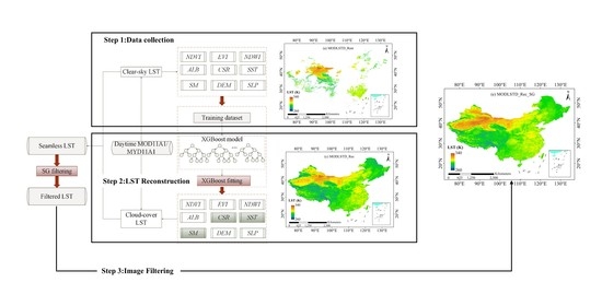
Generating spatiotemporally continuous land surface temperature (LST) data is in great demand for hydrology, meteorology, ecology, environmental studies, etc. However, the thermal infrared (TIR)-based LST measurements are prone to cloud contamination with missing pixels. To repair the missing pixels, a new XGBoost-based linking approach for reconstructing daytime and nighttime Moderate Resolution Imaging Spectroradiometer (MODIS) LST measurements was introduced. The instantaneous solar radiation and two soil-related predictors from China Data Assimilation System (CLDAS) 0.0625°/1-h data were selected as the linking variables to depict the relationship with instantaneous MODIS LST data. Other land surface properties, including two vegetation indices, the water index, the surface albedo, and topographic parameters, were also used as the predictor variables. The XGBoost method was used to fit an LST linking model by the training datasets from clear-sky pixels and was then applied to the MODIS Aqua-Terra LSTs during summer time (June to August) in 2017 and 2018 across China. The recovered LST data was further rectified with the Savitzky–Golay (SG) filtering method. The results showed the distribution of the reconstructed LSTs present a reasonable pattern for different land-cover types and topography. The evaluation results using in situ longwave radiation measurements showed the RMSE varies from 3.91 K to 5.53 K for the cloud-free pixels and from 4.42 K to 4.97 K for the cloud-covered pixels. In addition, the reconstructed LST products correlated well with CLDAS LST data with similar LST spatial patterns. The variable importance analysis revealed that the two soil-related predictors and the elevation variable are key parameters due to their great contribution to the XGBoost model performance.

Graphical Abstract

1. Introduction

Land surface temperature (LST) is a key parameter in environmental change, ecological processes and land-atmosphere energy exchange for different spatial scopes [1,2,3,4]. It enables monitoring of agricultural drought, urban heat, surface energy fluxes, and hydrological and meteorological processes [5,6,7,8,9,10,11], etc. In situ measurement is a credible source to acquire accurate LST data, but it is hard to obtain spatiotemporally continuous measurements for large-scale areas [12]. Satellite remote sensing has provided the unique approach to obtaining LST with satisfactory revisit cycle and global coverage [13,14]. Thermal infrared (TIR)-based methods, such as single-channel, split-window, and mono-window algorithms [13,15,16,17,18], have been widely used to retrieve satellite-based LST data. Passive microwave (PMW)-based approaches have also been used for LST estimation with the advantage of better measurements through clouds [19,20]. Compared with LST retrieval from PMW sensors, the TIR-based LST data has attracted more attention due to its finer spatial resolution and higher accuracy [13]. Many TIR-based LST products have been generated from different sensors, such as the Moderate Resolution Imaging Spectroradiometer (MODIS) [21], the FengYun-2 (FY-2) Visible Infrared Spin Scan Radiometer (VISSR) [22], and the Meteosat Second Generation (MSG) Spinning Enhanced Visible and InfraRed Imager (SEVIRI) [23], etc. However, the data availability of TIR-based LST products is hampered by clouds or cloud shadows because TIR signals cannot penetrate thick clouds. The presence of clouds hinders the full spatial coverage of LST measurements, which greatly restricts the subsequent applications in many fields [24].
There have been many approaches to recovering the missing information and to enhancing the usability of incomplete LST products. These approaches are generally categorized into three types based on their different reference sources: (1) spatial information-based, (2) multi-temporal observation-based, and (3) spatial-temporal information-based [25,26]. The most widely-used methods are based on spatial information. For example, Jin [27] proposed a neighboring-pixel (NP) approach for calculating the missing LST information based on the surface energy balance (SEB) theory. Many spatial interpolation approaches, such as geostatistical methods were also proposed to fill cloud-covered pixels [28,29]. However, the recovered regions often yield unsatisfactory accuracy and blurred results when only the spatial information was considered. The multi-temporal information-based methods which utilize the information of time sequence images have also been well developed. These approaches include the linear temporal approaches [30,31], the harmonic analysis of time-series (HANTS) method [32], the Savitzky–Golay (SG) filtering method [33,34,35], the diurnal temperature cycle (DTC) method [36,37], and the annual temperature cycle (ATC) method [38,39], etc. Such approaches are appropriate for LST images with adequate pixels and sufficient multi-temporal information, but generally ignore information from geographically neighboring information and thus are only suitable for the images with regular variation [25]. In other words, such approaches are very sensitive to abrupt changes caused by land-cover change or sudden natural disasters [40]. The third category are the spatiotemporal methods, i.e., hybrid methods, which take both the spatial and temporal information into account. Several temporal NP approaches were developed to reconstruct cloud-contaminated LSTs [41,42]. A two-step MODIS LST reconstruction procedure was also developed by using multiple LST images with vegetation index and the SEB-based correcting procedure [12]. Besides, some spatial-temporal fusion techniques and the convolutional neural network have been introduced to generate high-resolution seamless LSTs [43,44]. The spatiotemporal reconstruction method is suitable for filling large data-missing regions with high accuracy and at reasonable computational cost. However, such methods still underutilize the available spatial and temporal information, thus there is room for further maximizing the availability of all available spatiotemporal information [25]. For example, Yao et al. [45] proposed an enhanced hybrid method that fused spatiotemporal information with information from other similar LST products to recover MODIS and Visible Infrared Imaging Radiometer Suite (VIIRS) LST products.
Despite the achievements made on the reconstruction of satellite-based LST products, limitations still exist. The first one is that most of the studies have paid attention on the reconstruction of daytime LST [26]. Few studies have been performed to recover daytime and nighttime MODIS Aqua-Terra LST products simultaneously. Nighttime LST reconstruction has been limited to a few studies that merged the information from PMW-based data due to its low susceptibility to water vapor and cloud influence [46,47,48,49,50,51,52]. However, a wide scanning gap between orbits for PMW data and its relatively low spatial resolution (tens of kilometers) often lead to the unsatisfactory fusion results [25]. Another limitation is the lack of evaluation for different land-cover types of reconstruction results in previous studies. The spatial pattern of LST is directly affected by different land-cover types [53,54]. Therefore, it is necessary to assess the reconstructed LST products for different land-cover types. Additionally, LST is synthetically affected by many factors, such as land-cover types, topographic parameters, soil parameters, and atmospheric forcing conditions [26,55,56,57]. Nevertheless, the influence of soil parameters (e.g., soil surface temperature (SST) and soil moisture (SM)) on LST or their interrelation has not been evaluated.
To address the abovementioned limitations, the purpose of this study is to develop a more practicable approach for reconstructing all-weather LST for cloud-covered pixels of the MODIS Aqua-Terra LST products. Considering that incident solar radiation is the key factor for the equilibrium between incoming and outgoing energy and determines the final LST values, Zhao et al. [26] used a modified random forest (RF) linking model proposed by Zhao et al. [58] to reconstruct daytime MODIS LST product. The RF linking model was conducted to link daytime LST with the solar radiation factor and other explanatory factors. However, the incident solar radiation made a small contribution in establishing the RF linking model of Zhao et al. [26], thus more appropriate variables need to be adopted to make the model more convincing. On the other hand, their developed RF linking models are only suitable for the reconstruction of daytime LST. In this study, in addition to the solar radiation factor, the instantaneous soil-related properties (SST and SM) were also considered as the key linking variables. The eXtreme Gradient Boosting (XGBoost) machine learning (ML) model, with its capacity of large-scale data modeling, was used to construct the relationship between LST with soil properties and other land surface properties (vegetation indices, water index, surface albedo, solar radiation and topographic parameters). Then, the built model was applied to the missing pixels to acquire the LST estimates and used for spatially continuous LST mapping over China. Finally, the reconstructed results were evaluated against LST measurements from China Meteorological Administration (CMA) and ground measurements in the Heihe River Basin, and additionally compared with China Land Data Assimilation System (CLDAS) LST data.
The major objectives of this study are to: (1) introduce an XGBoost-based algorithm to repair the missing information of daytime and nighttime MODIS Aqua-Terra LST data simultaneously; (2) assess whether the reconstructed LST results present the reasonable patterns for different land-cover types; (3) evaluate whether the accuracy of the reconstructed LST products meets the requirement compared with other studies, and (4) explore variable importance of each predictor and prove the rationality of the variable selection.

2. Study Area and Data

2.1. Study Area

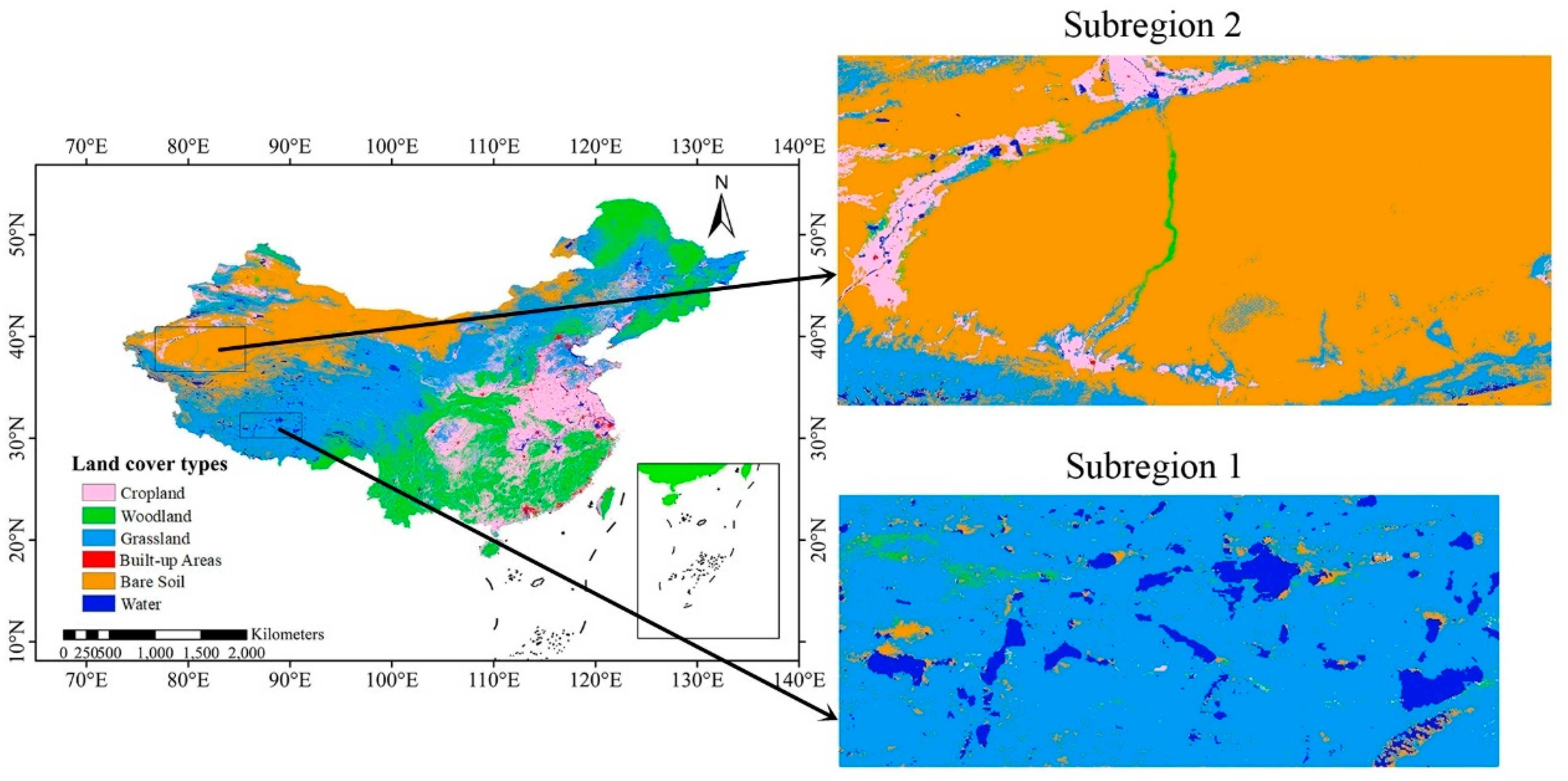
China is selected as the study area (Figure 1). With an area of approximately 9.6 million km2, China lies between latitudes 3° N and 54° N, and between longitudes 73° E and 136° E. The map of land-cover types in China is shown in Figure 1. The 300 m land-use cover product in 2018 generated from European Space Agency (ESA) Climate Change Initiative (CCI) project was used in this study (http://maps.elie.ucl.ac.be/CCI/viewer/index.php). The land-cover data from ESA was resampled to a 1 km resolution by mode resampling and reclassified into six types including water, bare soil, built-up areas, grassland, woodland, and cropland, for the purpose to simplify the evaluation of the impact of different land cover on LST reconstruction performance. China features high spatial heterogeneity in land-cover types, where the plains and basins account for ~33% of the land area, while mountainous areas, hills and plateaus account for the other 67% of area. Due to the complicated terrain, the climate in China varies greatly in space and is mainly dominated by dry seasons and wet monsoon [59].

2.2. Datasets

2.2.1. MODIS Data

In this study, the MODIS Aqua-Terra daily LST products (i.e., MOD11A1/MYD11A1) were selected to reconstruct cloud-covered LSTs. The auxiliary data from MODIS products used as the predictive variables were the normalized difference vegetation index (NDVI), the enhanced vegetation index (EVI), the normalized difference water index (NDWI), and surface albedo.
The 16-day NDVI and EVI products were provided by the MODIS Aqua-Terra Vegetation Indices datasets (MOD13A2/MYD13A2). The NDWI were calculated from the surface reflectance product (MOD09A1) at an 8-day/500 m resolution and are given by
NDWI = ρ n i r ρ s w i r ρ n i r + ρ s w i r
where ρ n i r and ρ s w i r denote band 2 and band 5 of the MOD09A1 product, respectively.
The surface albedo data were derived from the albedo product (MCD43A3) at an 8-day/500 m resolution. The NDWI and surface albedo datasets were upscaled to 1 km resolution by pixel averaging to match MODIS LST data. All MODIS products were acquired from June to August in 2017 and 2018, and were obtained from the NASA Land Processes Distributed Active Archive Center (LPDAAC) (https://ladsweb.modaps.eosdis.nasa.gov/).

2.2.2. Reanalysis Data

The CMA (China Meteorological Administration) China Land Data Assimilation System (CLDAS) started to release the official products (Version 2.0, 0.0625° × 0.0625°) from 2008, and these products cover East Asia (0–65° N, 60–160° E). Meteorological fields used in the CLDAS land surface modeling (LSM) include hourly air temperature, air pressure, humidity, precipitation, solar radiation, surface temperature, shortwave radiation, soil surface temperature, and soil moisture, etc. The CLDAS reanalysis data are derived from LSMs using data fusion and assimilation methods [60,61].
In this study, the hourly CLDAS shortwave radiation, soil surface temperature (0–10 cm), and soil moisture (0–10 cm) were selected as the predictors of LST. As the CLDAS LST product proves to be well consistent with in situ LST [44], the CLDAS LST product was used to evaluate the reconstructed LST. In addition to the shortwave radiation parameter obtained during the daytime, CLDAS soil parameters at 11:00 a.m., 22:00 p.m., 2:00 p.m., and 2:00 a.m. (Beijing time) were selected to match the overpass time of MODIS Aqua-Terra products. These hourly reanalysis data in NetCDF format are publicly accessible from the China Meteorological Data Service Center (CMDC) at http://data.cma.cn.

2.2.3. Topographic Parameters

Topographic parameters affect variations in LSTs because of the varying atmospheric forcing environment and with the effect on the dispersion of incident solar radiation [26,62]. The DEM data was from the Shuttle Radar Topography Mission (SRTM) at a 90 m resolution and obtained from the Geospatial Data Cloud (http://www.gscloud.cn/). Then the slope data was calculated from the SRTM data, and the two topographic datasets were upscaled to 1 km resolution by pixel averaging.

2.2.4. Ground-Measured Data

Two ground-based datasets were used for the evaluation. One in situ measured LST dataset was obtained from “China’s surface climate data daily value data set (V3.0)” (http://data.cma.cn) provided by CMA. This dataset, which has been strictly quality-controlled, contains data from 699 benchmarks and basic automatic weather stations in China and provides daily maximum, minimum, and average land surface temperature (0 cm) measured by platinum resistance temperature sensor. The maximum permissible error is ± 0.2 °C (≤50 °C) or ± 0.5 °C (>50 °C). The advantage of this dataset is that the stations cover the entire study area and can be used to evaluate the overall spatiotemporal characteristics of the reconstructed MODIS LST data. In order to make the station distribution more uniform, 200 automatic weather stations were randomly selected for verification by using the “Create Fishnet” module of ArcMap with a 2° × 2° cell (Figure 1).
Another dataset is the ground-based measurements from the Heihe Watershed Allied Telemetry Experimental Research (HiWATER) [63,64], a comprehensive eco-hydrological experiment conducted in the Heihe River Basin. This dataset measured by Net Radiometer CNR4 with a maximum nonlinear error of 1% has been used to assess the accuracy of the all-weather MODIS LST [49,65]. This dataset also has been quality-controlled. Five HiWATER sites (i.e., DSL, AR, HZZ, HH, and SDQ) provided by National Tibetan Plateau Data Center were used for verification (http://data.tpdc.ac.cn) in this study. Some details of these sites were displayed in Table 1. The ground-measured LSTs at the five sites were calculated from the upwelling and downwelling broadband hemispherical radiances by Stefan–Boltzmann’s law:
T s = [ F ( 1 ε b ) F σ ε b ] 1 / 4
where T s is the estimated LST, F is the downwelling longwave radiation, F is the surface upwelling longwave radiation, σ is the Stefan–Boltzmann constant (5.67 × 10⁻⁸ W m−2 K−4), and ε b is the surface broadband emissivity. The ε b was estimated from MODIS narrowband emissivity products using an empirical linear relationship [66]. Additionally, the “3σ-Hampel identifier” was adopted to reduce the influences from outliers [65,67].
Table 2 gives an overview of the datasets used in this study, including the variable types, dataset name/source, and the spatiotemporal resolution.

3. Methodology

3.1. Theoretical Context

LST is comprehensively affected by multiple factors, such as land-cover types, topographic parameters, soil parameters, atmospheric forcing conditions, etc. [26,55,56,57]. Thus, many studies have considered multiple related factors to express the relationship between LST and these auxiliary factors, and these built relationships have been further used for LST reconstruction [26,50,58], LST downscaling [75], etc. The key of building these models is to find the variables that change synchronously and are closely related to the LST parameter, such as the linking variable (i.e., incident solar radiation) in Zhao et al. [58] and Zhao et al. [26], and the Annual Cycle Parameters (ACPs) in Sismanidis et al. [76]. In this study, we evaluated the utility of several linking variables as proxies for instantaneous LST over China, and reconstructed daytime and nighttime LSTs from MODIS observations.

3.2. Extreme Gradient Boosting (XGBoost) Model

Several studies have successfully used an ensemble learning method (i.e., RF method) to reconstruct cloud-covered LSTs [26,51,52]. The XGBoost algorithm belongs to the Gradient Boosting Decision Tree (GBDT) algorithm, which is an iterative decision tree algorithm consisting of multiple decision trees [77], and the final decision is made by iterating multiple trees together. XGBoost represents an efficient GBDT algorithm enabling gradient boosting “on steroids” [78]. It combines advanced optimization techniques to produce excellent results while using less computing resources than other methods [79]. This study involved LST modeling over a large area (i.e., China), and it was feasible to use XGBoost algorithm modeling with vast amounts of LST pixels.

3.3. LST Reconstruction Based on XGBoost Linking Model

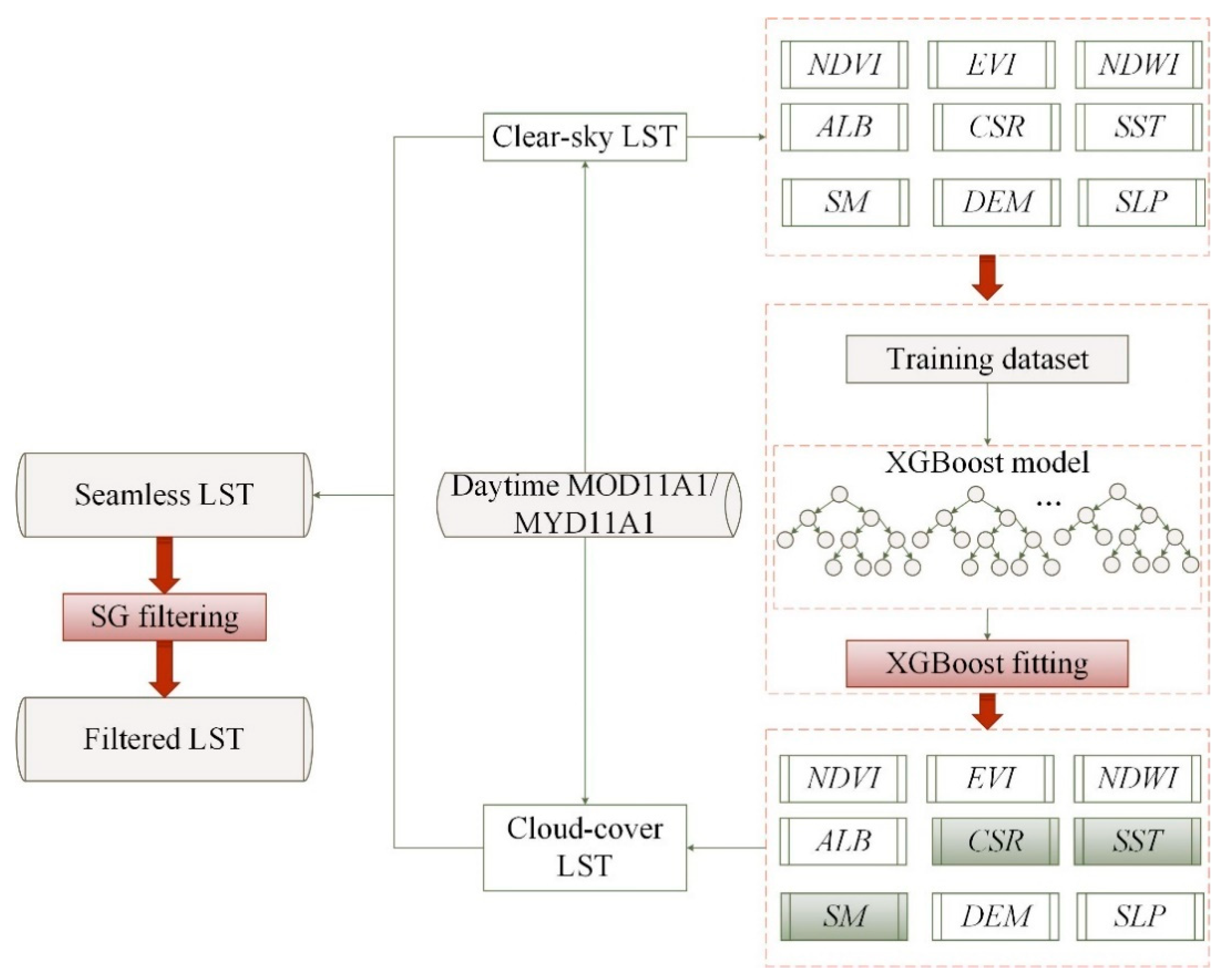
The RF linking model proposed by Zhao et al. [58] and Zhao et al. [26] is based on the assumption that incident solar radiation dominates the morning warming process and this factor can accurately represent the close relationship between the daily LST and surface solar radiation [26,58,80,81]. In this study, for daytime MODIS Aqua-Terra LST’s reconstruction, the incident solar radiation was also taken into account and was estimated by cumulating the CLDAS shortwave radiation data on surface warming process from sunrise time to satellite sunrise time. However, the cumulative incident solar radiation (CSR) is around zero during nighttime, thus the CSR cannot be used as an input to build a nighttime LST linking model, but the instantaneous CLDAS SST and SM data at an hourly resolution can be used as good proxies for daytime and nighttime LSTs due to their close relationships. Combined with other predictors based on Zhao et al. [26], including NDVI, EVI, NDWI, surface albedo (ALB), solar radiation, DEM, and slope (SLP), the proposed LST linking model based on XGBoost is expressed as follows:
{ T a c t _ d a y = T e s t _ d a y + e d a y T e s t _ d a y = F ( N D V I , E V I , N D W I , A L B , C S R , S S T , S M , D E M , S L P )
{ T a c t _ n i g h t = T e s t _ n i g h t + e n i g h t T e s t _ n i g h t = F ( N D V I , E V I , N D W I , A L B , S S T , S M , D E M , S L P )
where Equation (3) is the daytime LST linking model, and Equation (4) is the nighttime LST linking model with the CSR factor removed. T a c t _ d a y and T a c t _ n i g h t denote the actual daytime and nighttime LST respectively, T e s t _ d a y and T e s t _ n i g h t denote the estimated daytime and nighttime LST respectively, e denotes the estimation error of the linking model, and F is the function of an established XGBoost model. The process of the LST reconstruction is described as follows:
(1) Data Preprocessing: Before building the linking model, the quality control (QC) data of the MODIS Aqua-Terra LST products was used to remove pixel errors larger than 2 K to reduce the uncertainty derived from original LST data [26]. The NDVI or EVI data were compiled to generate two new time-series datasets with an 8-day resolution by combing the 16-day MOD13A3/MYD13A3 products. Then, all the MODIS-based datasets with an 8-day resolution (i.e., NDVI, EVI, NDWI, and ALB) were linearly interpolated to generate daily data. As for the hourly CLDAS-based predictors (i.e., SST and SM) with a 0.0625° resolution, they were downscaled to 1 km resolution using a bilinear interpolation method.
(2) LST Linking Model Building: The XGBoost model was adopted to fit the LST linking model and to construct the relationship between clear-sky LSTs and the predictors. It should be noted that the CSR variable was eliminated for the nighttime LST linking model. We used the XGBoost package in scikit-learn, and most parameters were set to the default except that the parameter “max_depth” was tuned from 10 to 20 and the parameter “n_estimators” was tuned from 100 to 250 following the changes of “max_depth” to avoid overfitting according to the root-mean-square error (RMSE) of the training dataset. The mean squared error (MSE) was selected as the loss function because it is commonly used in regression issue. The selected optimal parameters were determined by the trade-off of model accuracy and time consumption for the XGBoost training model.
(3) LST Reconstruction: Among the input datasets for fitting the linking model, the predictors of Equations (3) and (4), except for CSR, SST, and SM, are mostly invariant within a day. The three instantaneous predictors (i.e., CSR, SST, and SM) are used as critical proxy variables to link the clear-sky LST pixels and cloud-covered LST pixels via the established linking model. To produce the reconstructed LST, the built model was applied to the region with missing pixels.
(4) Seamless LST Postprocessing: MODIS data are influenced by undetected clouds and poor atmospheric conditions, which caused discontinuous data existing in MODIS data [82,83]. The change curve of original LST often demonstrates sudden plunges due to cloud and snow cover, which caused sudden drop points that were not in a good agreement with the overall trend [33]. The SG filtering method has been used to smooth and reconstruct the LST time-series data to reduce the noise data. Two key parameters must be determined. The first parameter is m that denotes the half-width window, and the other parameter is d that denotes the degree of the smoothing polynomial. In this study, the two parameters were set to 2 and 3 respectively, and the SG filtering was only applied to the outlier data with values lower than the overall trend [33].
The flowchart of the whole process for daytime LST reconstruction is shown in Figure 2, and the process for nighttime LST reconstruction is similar with the daytime LST reconstruction.

3.4. Validation

In this study, in situ measured LST data were used to evaluate the reconstructed LST results. Besides, the CLADS LST data were also adopted to evaluate the spatial patterns and LST magnitudes of the reconstructed results. Three commonly used criteria were selected for the validation, that is, the coefficient of determination ( R 2 ), the root mean square error ( R M S E ), and the B i a s . The three statistical metrics are calculated as follows:
R 2 = [ i = 1 n ( Y i Y ¯ ) ( O i O ¯ ) ] 2 i = 1 n ( Y i Y ¯ ) 2 i = 1 n ( O i O ¯ ) 2
R M S E = [ i = 1 n ( Y i O i ) 2 ] / n
B i a s = i = 1 n ( Y i O i ) n
where Y i denotes the reconstructed LST value and O i denotes the corresponding in situ measured LST value or CLDAS LST value; Y ¯ and O ¯ are mean values of Y i and O i , respectively.

4. Results

4.1. Building of the LST Linking Model

We reconstructed the daytime and nighttime MOD11A1/MYD11A1 data across China during summer time (June to August) in 2017 and 2018. Separate datasets including the LST data for each satellite overpass time and corresponding auxiliary data were independently imported into an XGBoost-based LST linking model. To verify the accuracy and stability of the model, a hand-out cross validation method was employed by randomly splitting the training datasets into 90% of the total datasets, and the remaining 10% of the datasets as the training dataset and test dataset, respectively. The parameter of “max_depth” was set to 18 and “n_estimators” was set to 200 as the best parameters according to the minimum MSE value for the test dataset and the computation time. Table 3 shows the performances of the training accuracy and test accuracy of the four established XGBoost models on day of year (DOY) 167 of 2018. The XGBoost-based models yield R2 from 0.97 to 0.98, and RMSEs ranging from 1.54 K to 1.79 K for the training dataset. The cross validation results demonstrated that the XGBoost models have comparable accuracy for both the training datasets and test datasets. The high R2 values with low RMSE and Bias for both model fitting and cross validation suggested a good performance of the XGBoost algorithm.

4.2. Demonstration of Reconstructed Daytime and Nighttime LSTs

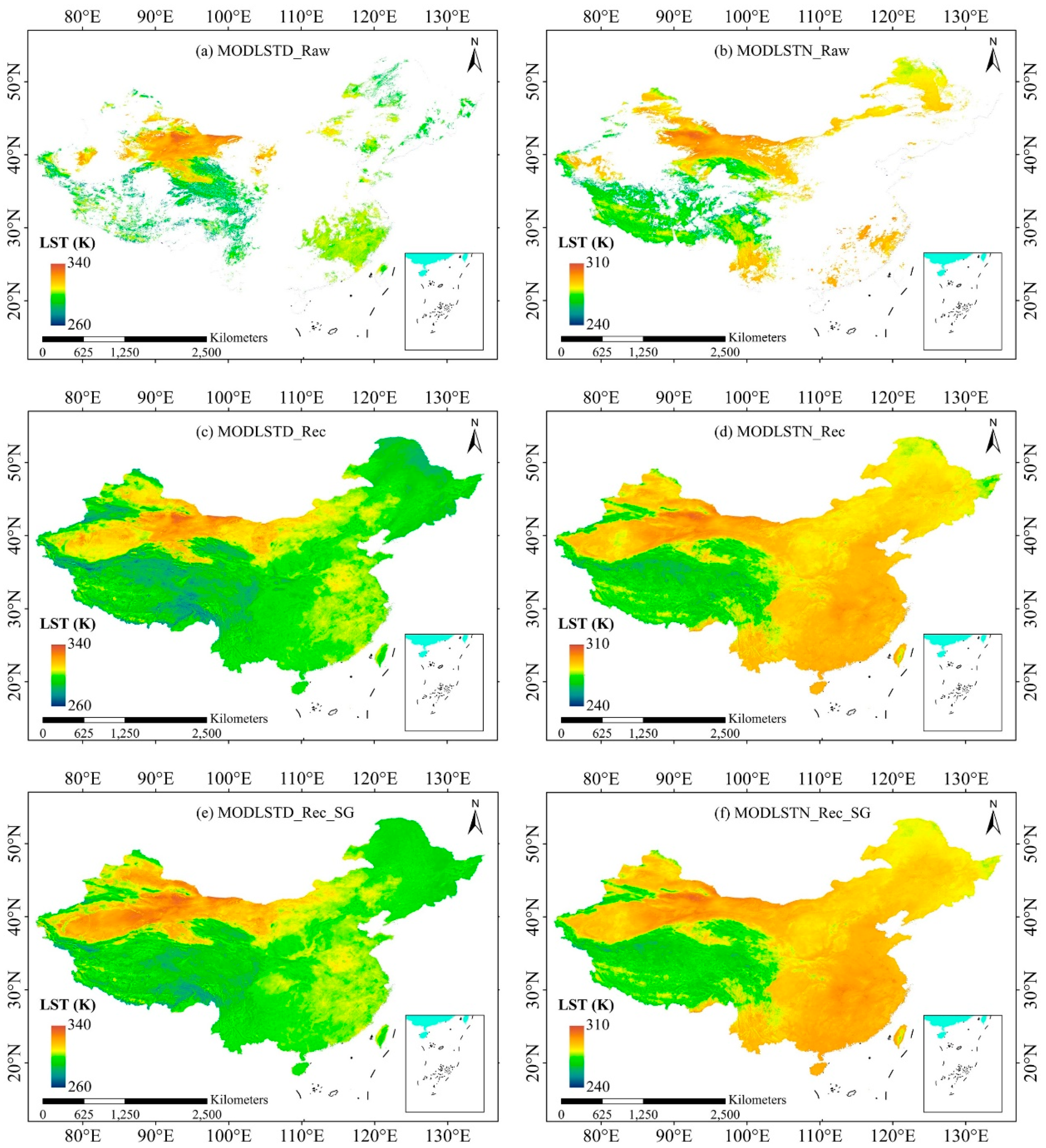
To facilitate the ease of reading, the original daytime LST and nighttime LST of MOD11A1 data, their corresponding reconstructed daytime LST and nighttime LST as well as reconstructed daytime LST and nighttime LST after SG filtering are labeled as MODLSTD_Raw, MODLSTN_Raw, MODLSTD_Rec, MODLSTN_Rec, MODLSTD_Rec_SG, and MODLSTN_Rec_SG, respectively hereafter, and so were the MYD11A1 data.
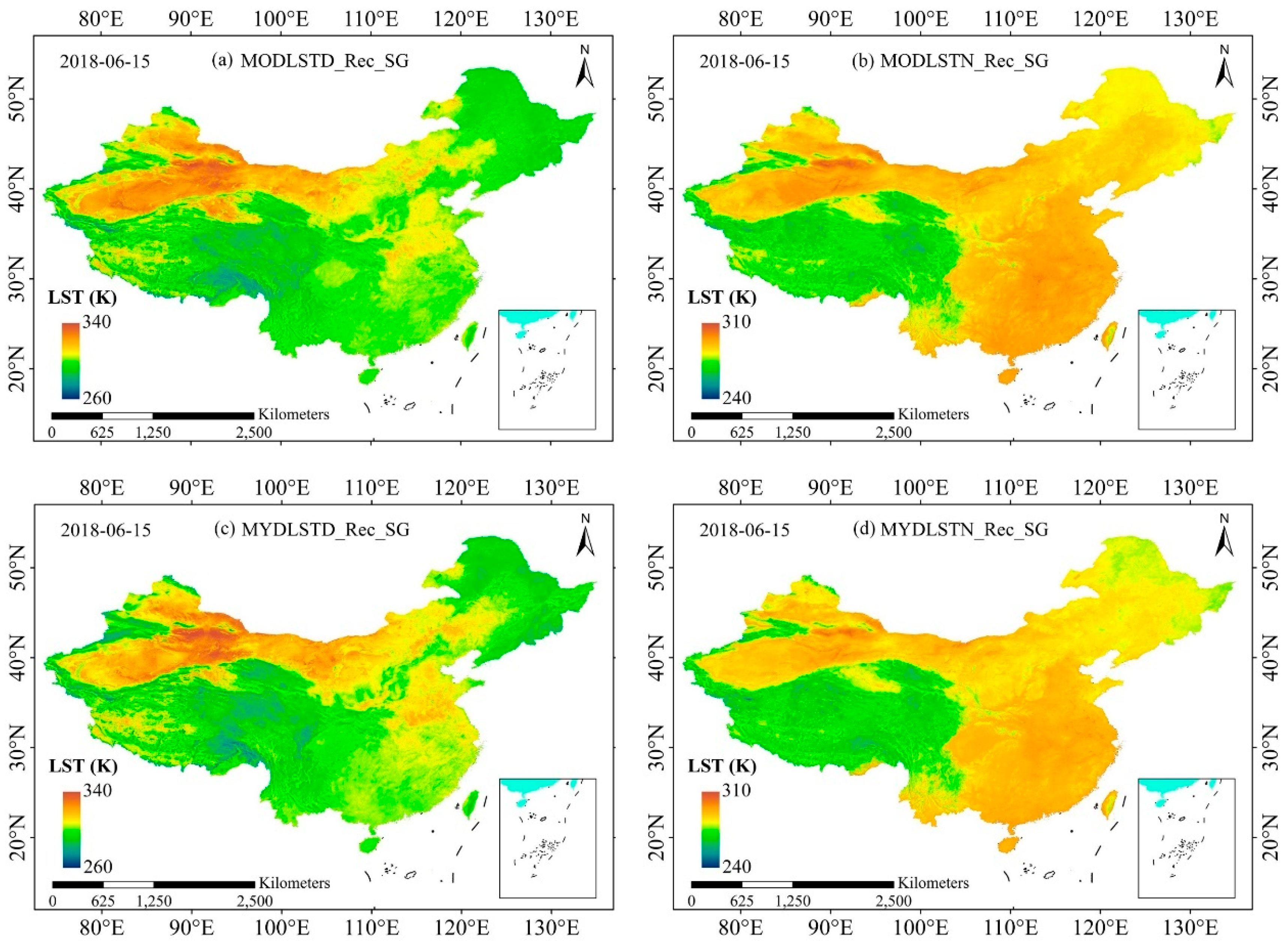
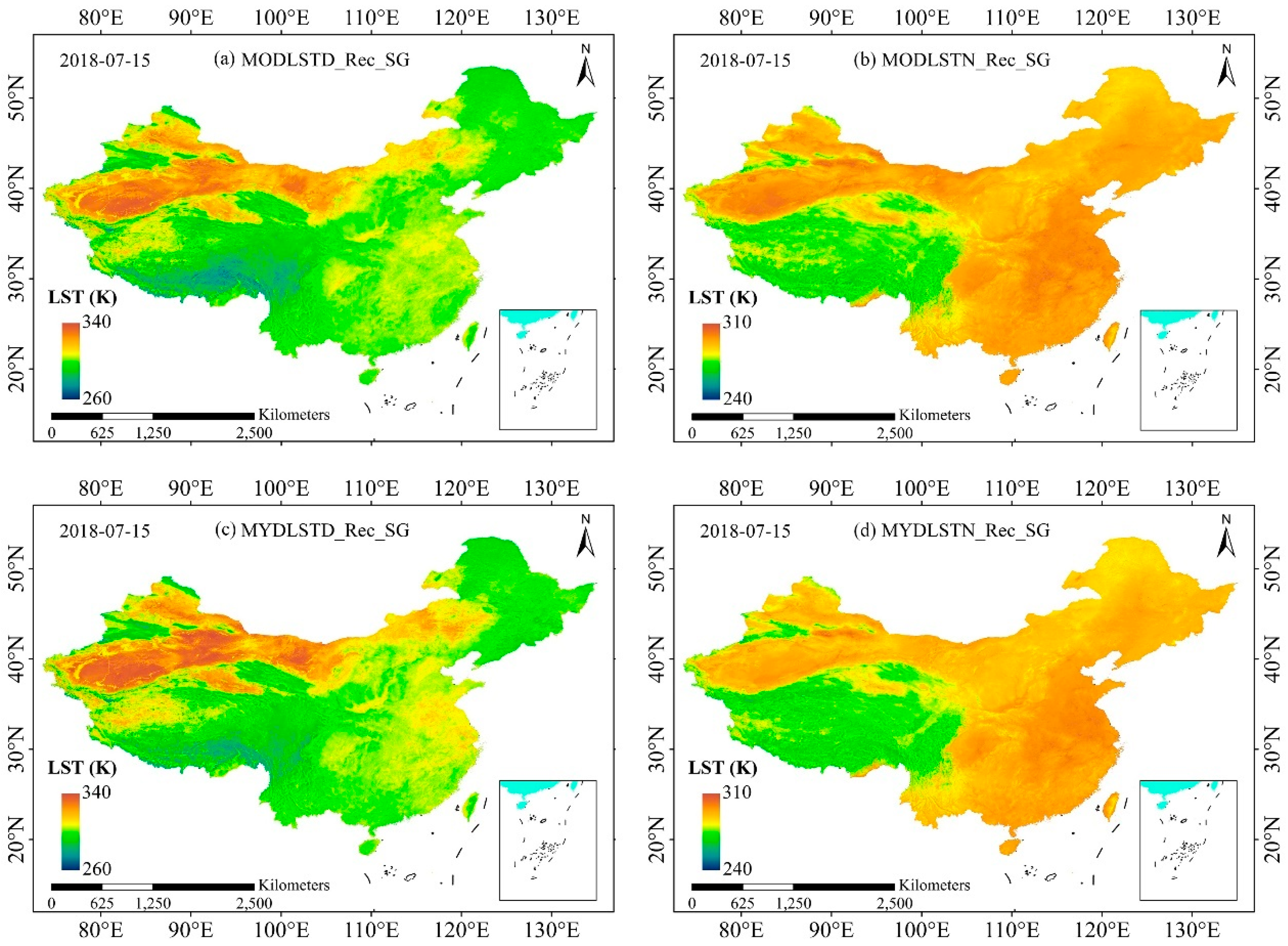
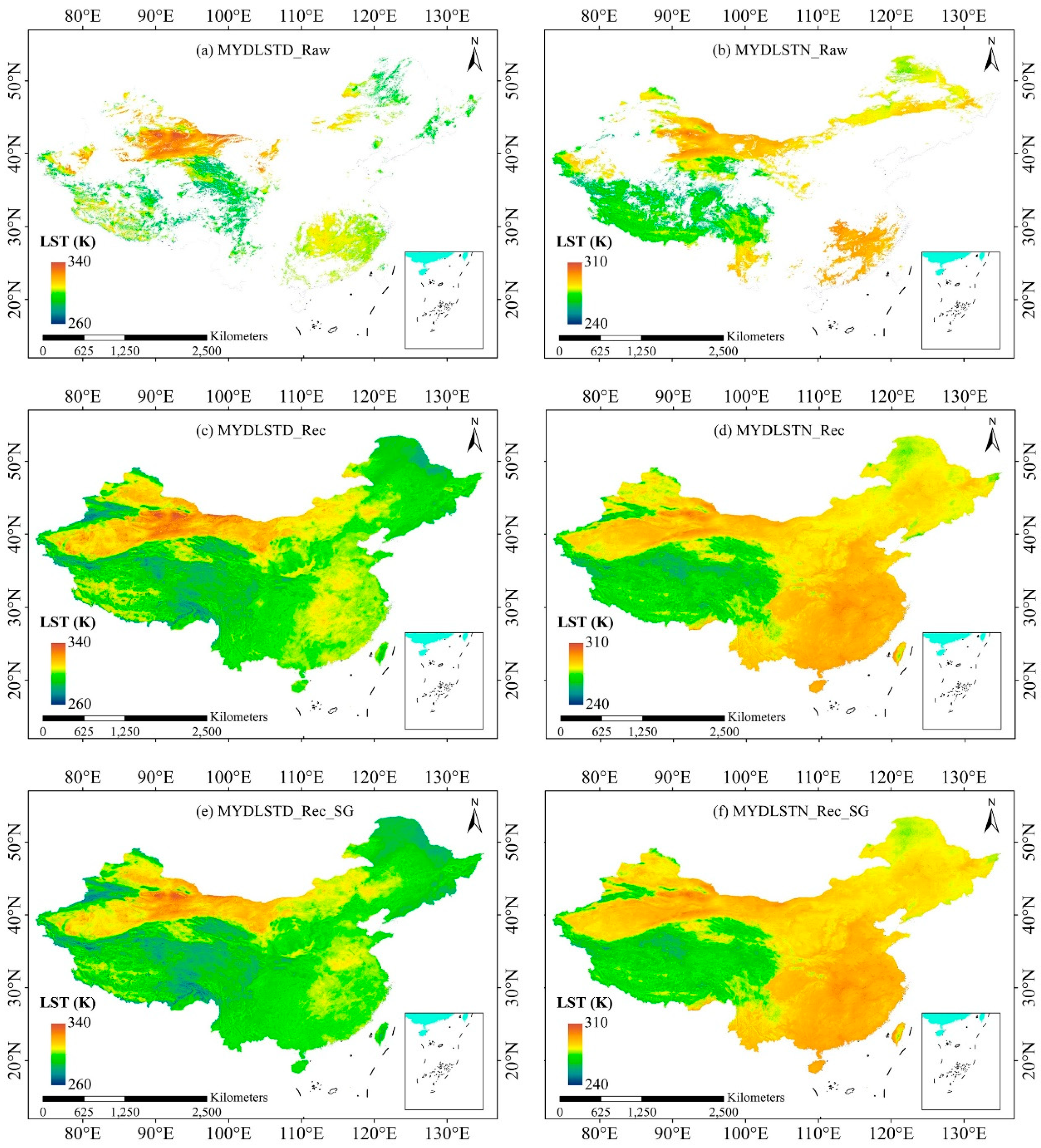
The original cloud-covered LST data of MODLSTD_Raw and MODLSTN_Raw on DOY 167 (June 16) of 2018 were displayed in Figure 3a,b, and their corresponding gap-filled LST data and reconstructed LST data with SG filtering were displayed in Figure 3c,d and Figure 3e,f, respectively. Likewise, the original cloud-covered MYD11A1 LST data and their corresponding reconstructed results were shown in Figure 4. Figure 3 and Figure 4 demonstrated that the XGBoost linking model can effectively fill a lot of missing LST pixels in the original LST images. The overall spatial patterns of the reconstructed LST images were consistent with the original LST data. More examples of reconstructed MODIS LST data on other days were provided in Figure A1, Figure A2 and Figure A3 in the Appendix A.

4.3. Reconstruction Effects for Different Land-Cover Types

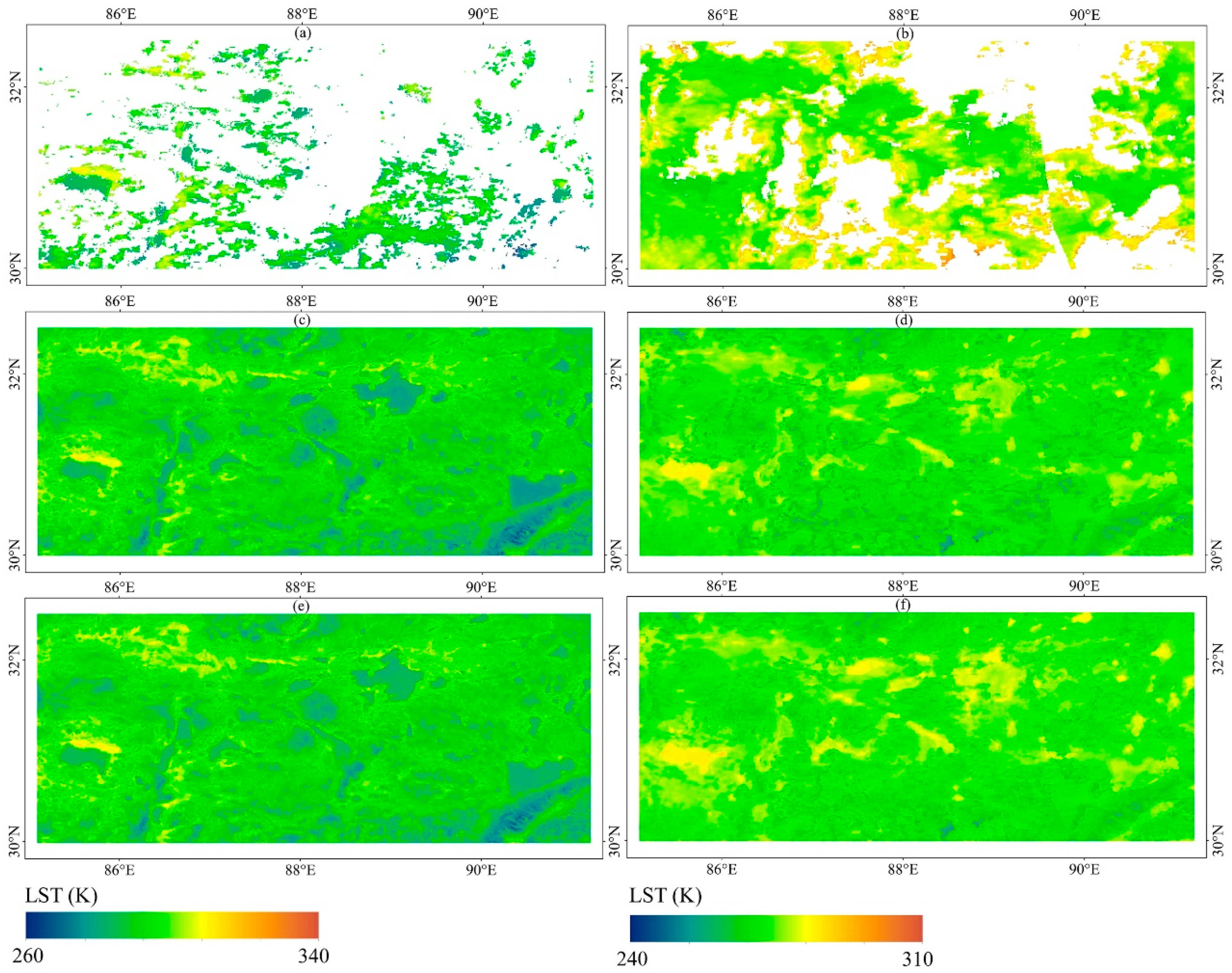
In order to show the reconstructed results in more detail, we selected two representative sub-regions, shown in Figure 5, as examples based on the reclassified land-cover types. Figure 6 shows the original MOD11A1 LST data and the corresponding reconstructed data on DOY 167 of 2018 for sub-region 1 scattered with water bodies. The daytime MODIS LST for pixels covered by water is usually lower than the surrounding pixels, and by contrast, the LSTs of nighttime water pixels are higher than the LSTs of their neighboring pixels. The reconstructed results (Figure 6c,d) can clearly reflect the terrain and land-cover information of the area with no obvious overestimation or underestimation. When the SG filtering was performed (Figure 6e,f), some underestimation and blurred information was rectified, though the improvement is not very evident for this sub-region.
Figure 7 displays the reconstructed results for sub-region 2 covered mostly by bare land, cropland, grassland, and woodland. Figure 7a,b show that the values of LST pixels covered with bare or sparsely vegetated land are higher than that of other land-cover types for both daytime and nighttime. Because of the large blank area in Figure 7a,b covered by bare soil or sparse vegetation, the surrounding relatively low LST pixels were used as input to the XGBoost model and then to estimate those missing pixels. Therefore, the corresponding reconstructed LSTs of Figure 7c,d were not so accurate with the underestimation effects. With the process of SG filtering via using the temporally adjacent LST information, the underestimated pixels were well rectified (refer to Figure 7e,f) by combining with the information of adjacent time-series LST data. Additionally, the step of SG filtering can restore the LST information in areas covered with other land-cover types (e.g., woodland) (Figure 7e vs. Figure 7c).

4.4. Validation with CMA Ground-Measured LST Data

The CMA ground-measured LST (0 cm) daily maximum, minimum, and average LST data was used to assess the reconstructed MODIS LST products. In this study, the daytime MYD11A1 LST and nighttime MYD11A1 LST were taken as proxies for the daily maximum and minimum LST, respectively. Additionally, we average the reconstructed daytime and nighttime MOD11A1 and MYD11A1 LST for each day to match the ground-measured average LST, and the average LST for both before and after SG filter processing were labeled as MODLSTAvg_Rec and MODLSTAvg_Rec_SG, respectively.
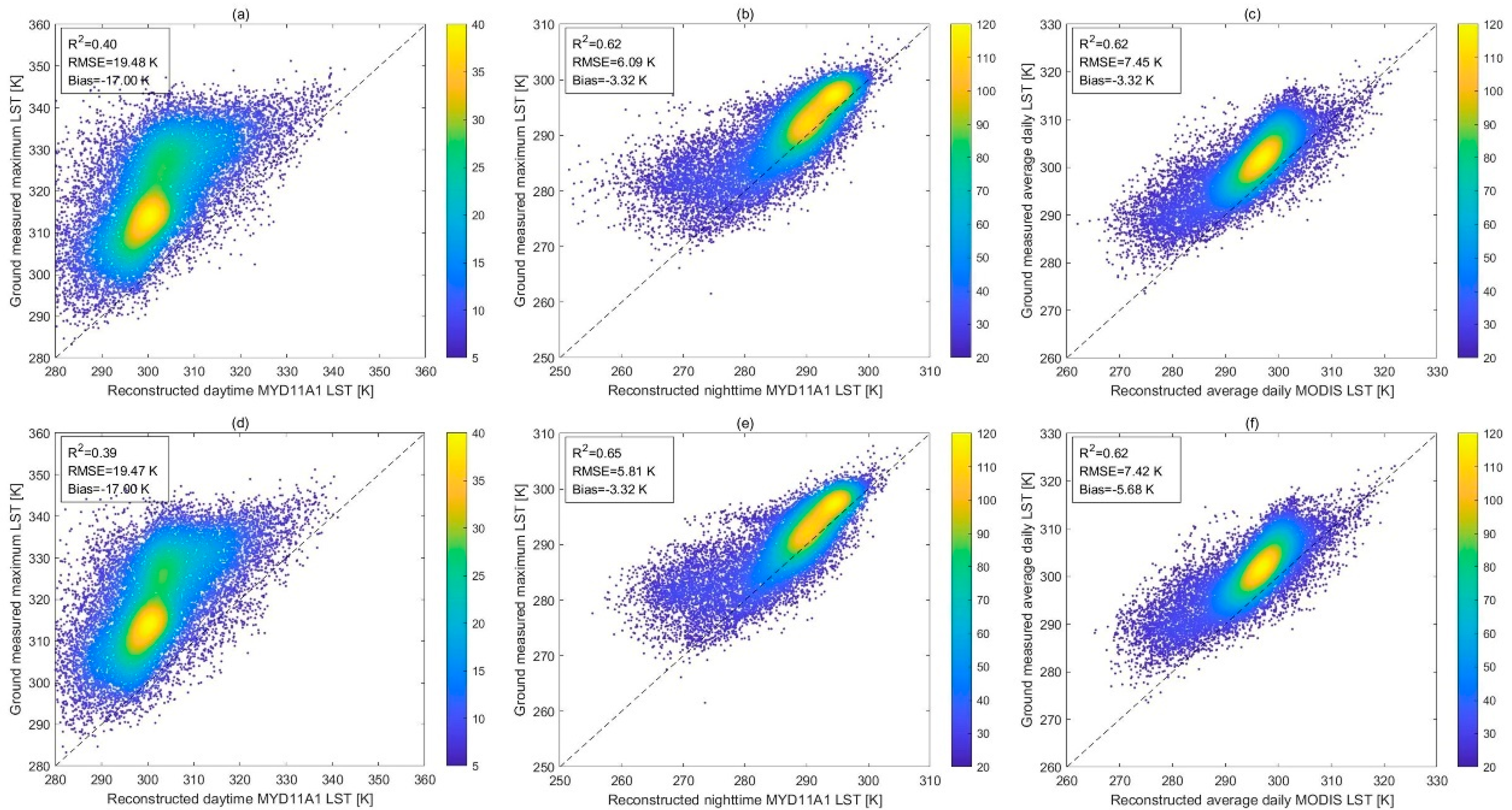
The validation results of the reconstructed MODIS LSTs (from June to August in 2017 and 2018) for both before and after SG filter processing were shown in Figure 8 and Figure 9. The distribution of density scatter points in Figure 8a and Figure 9a indicates that most of the LST values of the MYDLSTD_Rec data were far lower than the values of in situ measured maximum LST data (Bias = −17.00 K to −16.30 K). This suggests that the daytime MYD11A1 LST at local 2:30 p.m. does not give a good approximation of the daily maximum LST with relatively low R2 and high RMSE (R2 = 0.40 to 0.42, RMSE = 18.62 K to 19.48 K). Figure 8b and Figure 9b indicate that the nighttime MYD11A1 LST at local 2:30 a.m. correlated relatively well with the in situ measured daily minimum LST (R2 = 0.62 to 0.65, RMSE = 5.74 K to 6.09 K, Bias = −3.32 K to −3.18 K). The result of Figure 8c and Figure 9c indicate that the reconstructed daily average MODIS LST also has a relatively good correlation with the ground-measured mean LST (R2 = 0.62 to 0.63, RMSE = 7.07 K to 7.45 K, Bias = −5.37 K to −3.32 K). By comparison with the results of reconstructed LSTs with SG filter processing, we found little differences between Figure 8d–f and Figure 8a–c or Figure 9d–f and Figure 9a–c for the three statistical metrics, as the step of SG filter processing did not significantly change the original LST values. The values of RMSE and Bias were slightly altered (Figure 8d–f vs. Figure 8a–c or Figure 9d–f vs. Figure 9a–c), and the R2 value was improved from 0.62 to 0.65 (Figure 8e vs. Figure 8b) or from 0.65 to 0.68 (Figure 9e vs. Figure 9b) because the SG filter processing mainly improved the abnormally low LST values in the reconstructed LST products. From the results of the daily average LST, the R2 value was slightly reduced from 0.63 to 0.61 (Figure 9f vs. Figure 9c) or remained unchanged by comparing Figure 8f and Figure 8c. Thus, the step of SG filtering has little influence on the accuracy of the preliminary reconstructed LST product on the whole.
To further evaluate the accuracy for different land-cover types, Table 4 lists the validation of the reconstructed products for 6 land-cover types. The correlations for the three land-cover types of built-up areas, grassland, and cropland were higher than the other three land-cover types (i.e., water, bare soil, and woodland). In particular, for the reconstructed products of MYDLSTN_Rec_SG and MODLSTAvg_Rec_SG with the three land- cover types of built-up areas, grassland, and cropland, the R2 ranges from 0.59 to 0.80 during summer time in 2017 and 2018, the RMSE ranges from 2.41 K to 8.18 K, and the Bias ranges from −6.24 K to −0.91 K. The R2 for the other three land-cover types were relatively lower, while the RMSE ranges from 2.30 K to 9.21 K and the Bias ranges from −8.58 K to 0.56 K. As for the MYDLSTD_Rec_SG product, the poor validation results for all land- cover types were attributed to the large bias between the reconstructed MYDLSTD_Rec_SG and the in situ measured maximum LST data.

4.5. Validation Using HiWATER Data

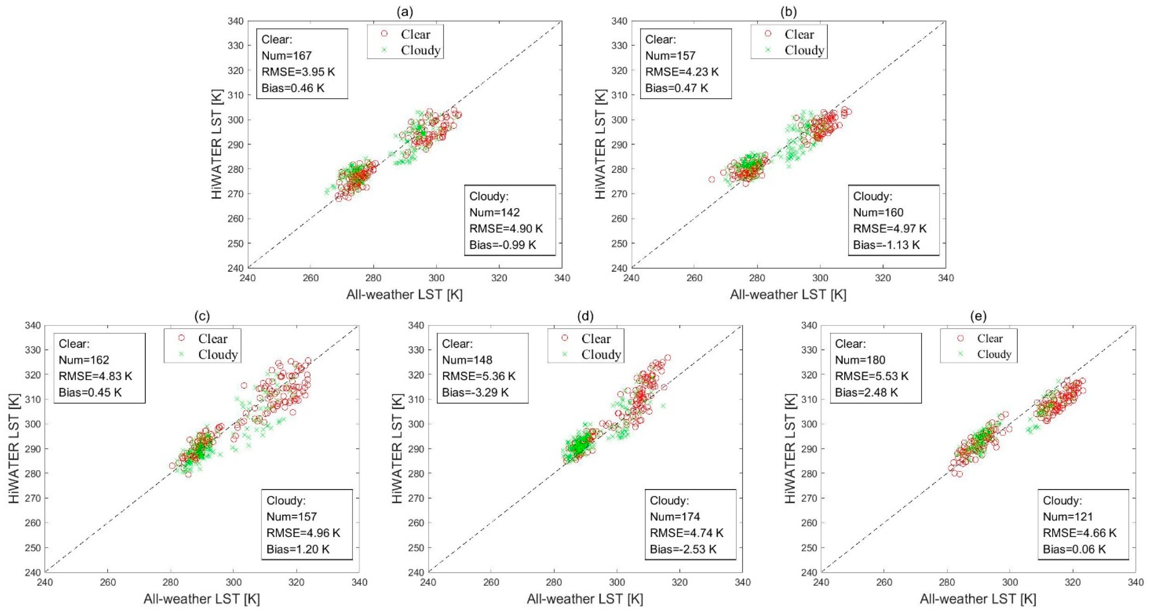
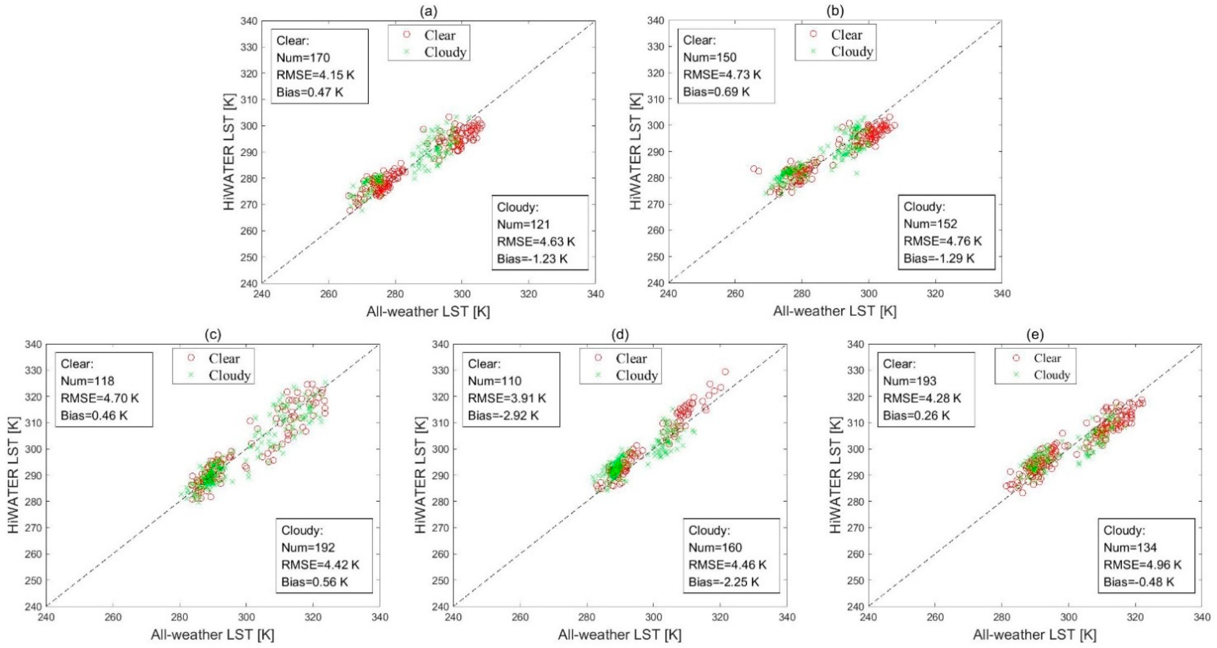
The accuracy of the all-weather LSTs were also evaluated against the HiWATER LST measurements at five sites and the results are shown in Figure 10 and Figure 11. The RMSE of the original cloud-free LST varies from 3.95 K to 5.53 K in 2017 and from 3.91 K to 4.75 K in 2018 at all sites. Duan et al. [49] pointed out that the spatial scale inconsistency between the pixel-wise all-weather LSTs and the point-wise in situ LSTs caused the relatively large RMSE. Another reason for this relatively low accuracy stemmed from the influence of cloud contamination. The accuracy evaluation used nearly all QC data rather than the best QC data (QC = 0) [49]. Thus, the accuracy of the all-weather LST is obviously lower than the nominal accuracy (1 K) of the MODIS LST product. From Figure 10 and Figure 11, the accuracy of the final reconstructed cloud-covered LST shows no distinct difference comparing to that of the cloud-free LST. The RMSE values range from 4.66 K to 4.97 K in 2017 and from 4.42 K to 4.96 K in 2018, and the Bias values range from −2.53 K to 0.06 K in 2017 and from −2.05 K to 0.56 K in 2018. Overall, the validation results demonstrated the consistent performance of the approaches used in this study.

4.6. Comparison with CLDAS LST Data

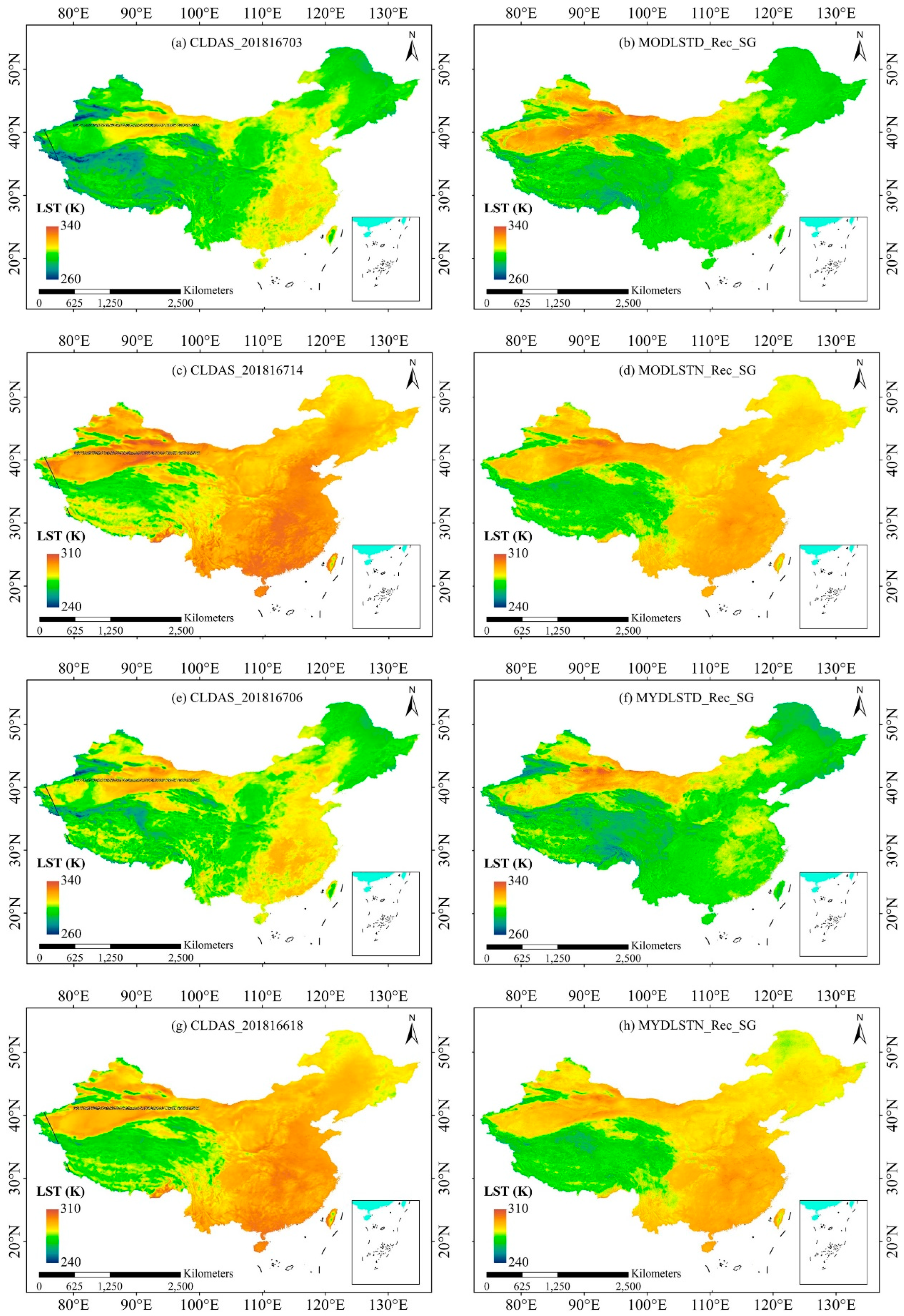
Taking the reconstructed results on DOY 167 of 2018 as an example, we compared them with the corresponding CLDAS LST products with an hourly/0.0625° resolution. The left column of Figure 12 shows the four CLDAS LST products and the right column shows the reconstructed results on DOY 167 of 2018. It is shown that the CLDAS LST products contain some missing pixels and noise data to the west of China. The reconstructed LST products depicted more detailed spatial information than the CLDAS LST, especially in areas with complex terrain (e.g., Tibetan Plateau). Overall, the reconstructed LST data had similar spatial variation with the CLDAS LST data. Differences in the LST magnitude are seen in some areas. For example, the reconstructed daytime MODIS LST data (Figure 12b,f) in northwest China were higher than those of the daytime CLDAS LST data (Figure 12a,e). In contrast, the LST estimates of Figure 12b,f in southeast China were lower than those of Figure 12a,e. For the nighttime LST data, the differences between the reconstructed MODIS LST data (Figure 12d,h) and CLDAS LST data (Figure 12c,g) were much smaller compared to the daytime LST data.
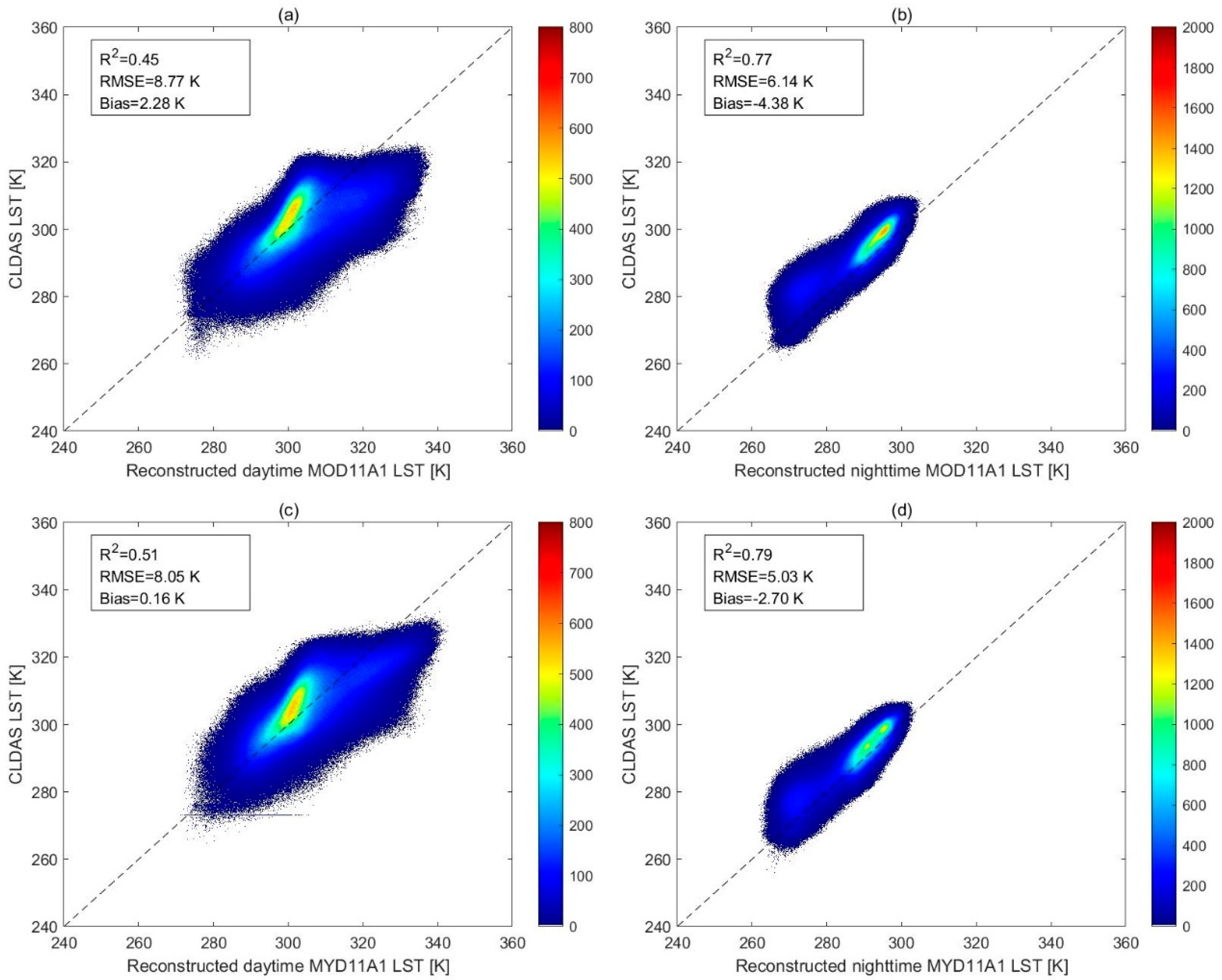
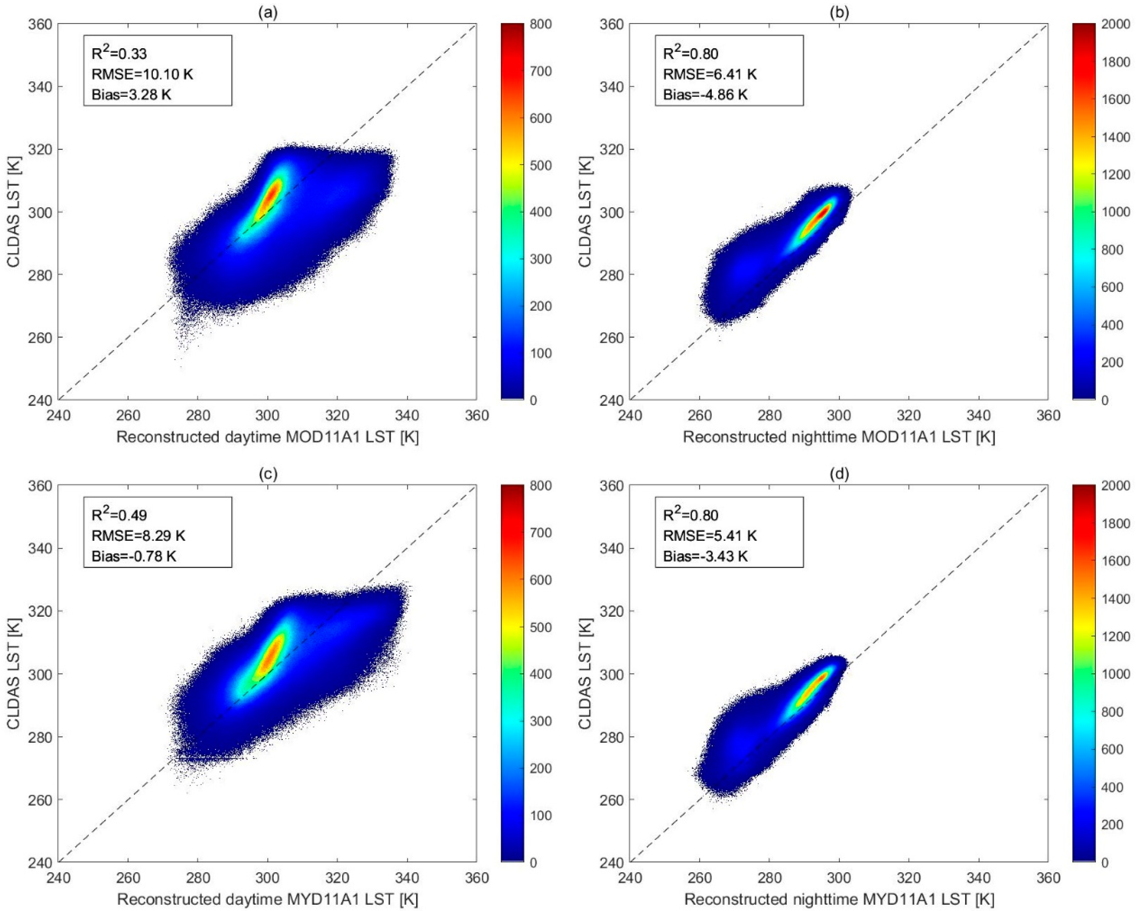
The reconstructed LST products were aggregated to 0.625° and matched-up to the CLDAS LST pixels by average aggregating to further understand the correlation between the reconstructed LST products with the CLADS LST products. Figure 13 and Figure 14 show the density scatter plots for the reconstructed LST data and the CLADS LST data from June to August in 2017 and 2018. From Figure 13 and Figure 14, some high outliers are seen in both daytime and nighttime LST estimates from CLDAS. The correlation between these two LST datasets varies (R2 = 0.33 to 0.80), while the correlation of nighttime LST data (R2 = 0.77 to 0.80) is significantly higher than that of the daytime data (R2 = 0.33 to 0.51). The RMSEs are relatively large for daytime estimates (RMSE = 8.05 K to 10.10 K), while the absolute Bias is smaller than 5 K for both daytime and nighttime estimates.

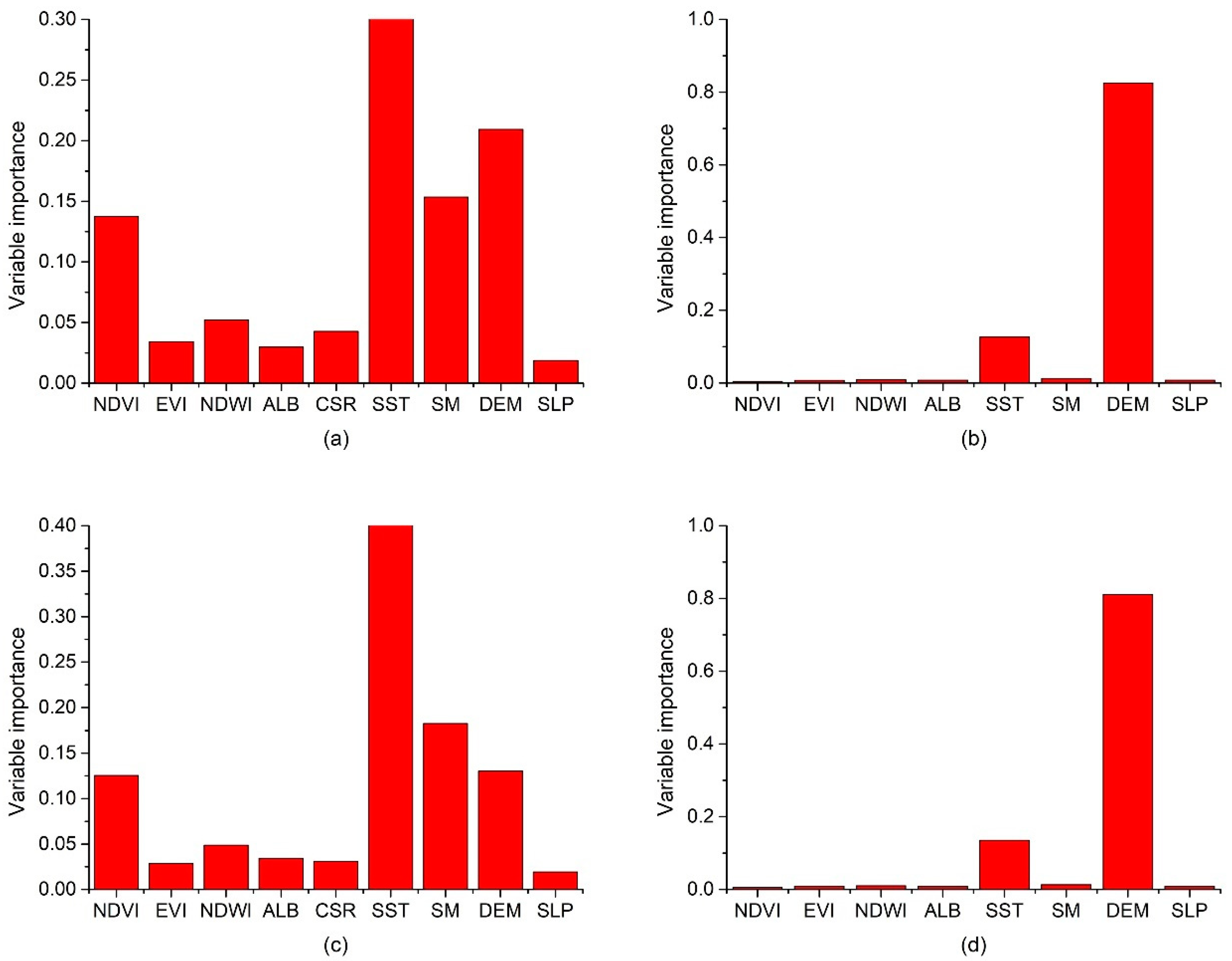
4.7. Variable Importance Analysis

The XGBoost algorithm enables assessment of variable importance to rank their contributions to the established model. The average importance of each predictor for the built XGBoost models during summer time in 2017 and 2018 in this study is shown in Figure 15. Figure 15 demonstrates that the variable importance differs with satellite overpass time. For daytime LST estimation, predictors such as SST, SM, DEM, and NDVI provided significant contributions to the XGBoost models (Figure 15a,c). For nighttime LST estimation, the three variables of DEM, SST, and SM exhibit more importance than the other variables (Figure 15b,d). The variables of SST, SM, and DEM are key inputs in the XGBoost models for both daytime and nighttime LST estimates due to their large contributions. Some studies have explored the relationship between SST and LST to retrieve SST [84,85], and Zhang et al. [51] even used SST data to validate the fused all-weather LST. Sun et al. [56] estimated the effects for SM on the retrieval accuracy of LST, and Jiang et al. [86] estimated hourly SM by using downscaled LST over different urban surfaces. For DEM data, Zhao et al. [26] pointed out there is a notable decreasing trend for surface elevation with LST due to the altitudinal temperature gradients. In the study area, surface elevation is also significantly correlated negatively with LST for both daytime and nighttime.

5. Discussion

5.1. Comparison with Other Studies

The reconstructed MYD11A1 LST data did not agree well with the CMA LST measurements for daytime data. One reason is that there was a difference between the satellite overpass time of MODIS LST data across China and the measurement time for CMA LST data. The gap time inevitably led to the large difference. On the other hand, Jiang et al. [87] compared the 0 cm LST measured by mercury thermometer with the LST retrieved by upward and downward longwave radiation in Tibetan Plateau. Based on the results, the highest difference in daytime is over 16 K so the results in this study were consistent with those of Jiang et al. [87]. The reason is that the measurement error of mercury thermometer is discrete and non-proportional, thus the representation of the LST measured by mercury thermometer is poor, even making the average or integral process [87]. It is essential to popularize the surface temperature measurement method based on the surface radiation to meet the demand of higher accuracy and reliability [87]. However, although this CMA dataset also has inherent systematic bias, the reconstructed nighttime MYD11A1 LST data correlated well with the CMA LST measurements, which demonstrated the good spatiotemporal continuity and relative accuracy of the reconstructed nighttime MODIS LST products.
Validation against radiation-based LST revealed stable performance at all five HiWATER sites, and the accuracy assessment was in line with previous studies. For example, the NP-based approach used by [42] was evaluated with two sites in Africa with the RMSE ranging from 5.11 K to 5.55 K. Duan et al. [49] merged TIR and PMW measurements in China with the RMSE varying from 3.5 K to 4.4 K. The study of Zeng et al. [12] showed the Mean Absolute Error (MAE) ranged from 3–6 K at six sites in America. Pham et al. [88] obtained the gap-filling MYD11C1 LST over Australia with the RMSE ranging from 2 K to 6.4 K at four stations in America. Here, the reconstructed MODIS data using the XGBoost method reached an RMSE between 3.91 K to 4.97 K, demonstrating an overall good performance with respect to the absolute accuracy.
Zhao et al. [58] proposed an RF linking model to reconstruct MODIS LSTs over a 120 km × 200 km study area (24,000 km2), and Zhao et al. [26] developed this initial RF linking model to recover daytime MODIS LSTs over a region of Southwest Europe (approximately 600,000 km2). Like RF, XGBoost can also handle complex nonlinearity relationships and address the multi-collinearity effect with high accuracy [89]. However, presently, it is hard for RF to process with tens of millions of training data by using existing RF packages, while XGBoost combines software and hardware optimization techniques to make it feasible and easier to study such large-scale study areas (i.e., China). Besides, the solar radiation factor variable, as the unique linking variable in Zhao et al. [58] and Zhao et al. [26], only makes a small contribution to the built models and is limited to the daytime as well. In this study, the variable importance analysis demonstrated the rationality of variable selection for the two soil-related linking variables due to their great contributions to the proposed XGBoost models.

5.2. Advantages and Limitations of the Proposed Method

TIR-based LST products are often contaminated by frequent cloud cover with missing pixels in large areas. Thus, we develop an XGBoost-based model to generate spatially continuous MODIS Aqua-Terra LST datasets over a large study area. First, the reconstructed results demonstrated the applicability and effectiveness of the XGBoost linking model to recover both daytime and nighttime LSTs. This reconstructed model is convenient to implement because it does not need much complex and prior parameter knowledge. Second, the XGBoost method had a strong fitting and predictive ability as no obvious fluctuation phenomenon existed in the reconstructed LST values. The proposed model can accurately restore LST with some fine object features such as water bodies (lakes and rivers). Third, the variable importance analysis also revealed the validity for the use of the two instantaneous soil-related variables (i.e., SST and SM) as the linking predictors between cloud-free LSTs and cloud-covered LSTs. The usage of them can facilitate the consideration of soil-related variables when restoring the TIR-based LST parameters.
However, there are still some limitations in this study. First, the preprocessing step for auxiliary variables had some inherent uncertainty. The disaggregation of 8-day MODIS-related auxiliary variables was performed using linear decomposition. Differences exist between the disaggregated results and their true values, though the differences may be ignored. In addition, the soil-related predictors were downscaled by a bilinear interpolation method, which led to relatively smooth results of reconstructed LSTs in areas where a large number of pixels were missing. Second, the SG filter processing cannot fully address the underestimation in the original MODIS LST data. The final reconstructed LST data still have some underestimated values. Third, the spatial scale inconsistency between in situ measured LST data and MODIS LST pixels with a 1 km resolution was not considered in the verification. The in situ measured LST data were required within a very small area while satellite measurements are the integrated responses over a heterogeneous surface. It may cause large uncertainty when the scale inconsistency is ignored in heterogeneous areas.

6. Conclusions

The quality of TIR-based LST data were greatly affected by frequent cloud cover, which severely restricted their applications in many related scientific fields. Therefore, to explore a practical method for the reconstruction of missing data in TIR-based LSTs is of great significance. In this study, an advanced method was adopted to reconstruct the missing information resulting from cloud cover in MODIS Aqua-Terra daytime and nighttime LST products. The instantaneous solar radiation and soil-related predictors obtained from CLDAS data were used as the linking variables to establish the relationship with instantaneous cloud-free LST data. By coupling with other predictors, we developed an XGBoost-based linking model to fit the complex relationship between cloud-free LST and the predictors, and then the constructed linking model was applied to the areas with cloud-covered pixels to generate spatially continuous MODIS LST estimates during summer time (June to August) in 2017 and 2018 across China. The SG filter method was adopted to further improve the quality of the reconstructed LST products.
The reconstructed LST products were validated and compared with daily in situ measured LST observations and CLDAS LST data. The validation results based on CMA stations showed that the nighttime and daily average LSTs agreed well with in situ data, while the daytime LST estimates showed poorer correlation due to the measurement error for platinum resistance temperature sensor. Evaluation for 6 different land-cover types led to similar conclusions. Besides, the validation results based on in situ LST measurements at five sites in the Heihe River Basin showed that the RMSE values ranged from 3.91 K to 5.53 K for the cloud-free LST and from 4.42 K to 4.97 K for the LST under cloud conditions. The accuracy of the reconstructed LST products meets the requirement comparing with other studies. The comparison with CLDAS LST data also showed similar LST spatial patterns, despite some difference in LST magnitudes.
The variable importance analysis revealed that the soil-related predictors (i.e., soil surface temperature and soil moisture) and the DEM variable made great contributions to the XGBoost model for both daytime and nighttime observation data, which could be used as a reference for the selection of predictors in the reconstruction of TIR-based LST data.

Author Contributions

Conceptualization and writing, W.T., C.W. and Y.L.; methodology and validation, W.T.; project administration and funding acquisition, D.X. All authors have participated in the manuscript revision. All authors have read and agreed to the published version of the manuscript.

Funding

This research was funded by the National Natural Science Foundation of China (grant numbers 42001178 and 41930646) and by Innovation Group Project of Southern Marine Science and Engineering Guangdong Laboratory (Zhuhai) (grant number 311021018).

Institutional Review Board Statement

Not applicable.

Informed Consent Statement

Not applicable.

Data Availability Statement

The data set of Heihe Integrated Observatory Network is provided by National Tibetan Plateau Data Center (http://data.tpdc.ac.cn).

Conflicts of Interest

The authors declare no conflict of interest.

Appendix A

Figure A1. Reconstructed MODIS LST results on 15 June 2018.
Remotesensing 13 04723 g0a1
Figure A2. Reconstructed MODIS LST results on 15 July 2018.
Remotesensing 13 04723 g0a2
Figure A3. Reconstructed MODIS LST results on 15 August 2018.
Remotesensing 13 04723 g0a3

References

  1. Trigo, I.F.; Boussetta, S.; Viterbo, P.; Balsamo, G.; Beljaars, A.; Sandu, I. Comparison of model land skin temperature with remotely sensed estimates and assessment of surface-atmosphere coupling. J. Geophys. Res. Atmos. 2015, 120, 12096–12111. [Google Scholar] [CrossRef] [Green Version]
  2. Kustas, W.; Anderson, M. Advances in thermal infrared remote sensing for land surface modeling. Agric. For. Meteorol. 2009, 149, 2071–2081. [Google Scholar] [CrossRef]
  3. Tierney, J.; Russell, J.; Huang, Y.; Sinninghe-Damste, J.; Hopmans, E.; Cohen, A. Northern Hemisphere Controls on Tropical Southeast African Climate During the Past 60,000 Years. Science 2008, 322, 252–255. [Google Scholar] [CrossRef] [Green Version]
  4. Hansen, J.; Ruedy, R.; Sato, M.; Lo, K. Global Surface Temperature Change. Rev. Geophys. 2010, 48, RG4004. [Google Scholar] [CrossRef] [Green Version]
  5. Mildrexler, D.; Yang, Z.; Cohen, W.; Bell, D. A forest vulnerability index based on drought and high temperatures. Remote Sens. Environ. 2015, 173, 314–325. [Google Scholar] [CrossRef] [Green Version]
  6. Zakšek, K.; Oštir, K. Downscaling land surface temperature for urban heat island diurnal cycle analysis. Remote. Sens. Environ. 2012, 117, 114–124. [Google Scholar] [CrossRef]
  7. Stisen, S.; Sandholt, I.; Nørgaard, A.; Fensholt, R.; Jensen, K.H. Combining the triangle method with thermal inertia to estimate regional evapotranspiration—Applied to MSG-SEVIRI data in the Senegal River basin. Remote Sens. Environ. 2008, 112, 1242–1255. [Google Scholar] [CrossRef]
  8. Silvestro, F.; Gabellani, S.; Delogu, F.; Rudari, R.; Boni, G. Exploiting remote sensing land surface temperature in distributed hydrological modelling: The example of the Continuum model. Hydrol. Earth Syst. Sci. 2013, 17, 39–62. [Google Scholar] [CrossRef] [Green Version]
  9. Tomlinson, C.; Chapman, L.; Thornes, J.; Baker, C. Remote sensing land surface temperature for meteorology and climatology: A review. Meteorol. Appl. 2011, 18, 296–306. [Google Scholar] [CrossRef] [Green Version]
  10. Yao, R.; Wang, L.; Huang, X.; Niu, Z.; Liu, F.; Wang, Q. Temporal trends of surface urban heat islands and associated determinants in major Chinese cities. Sci. Total. Environ. 2017, 609, 742–754. [Google Scholar] [CrossRef]
  11. Yao, R.; Wang, L.; Huang, X.; Gong, W.; Xia, X. Greening in Rural Areas Increases the Surface Urban Heat Island Intensity. Geophys. Res. Lett. 2019, 46, 2204–2212. [Google Scholar] [CrossRef]
  12. Zeng, C.; Long, D.; Shen, H.; Penghai, W.; Cui, Y.; Hong, Y. A two-step framework for reconstructing remotely sensed land surface temperatures contaminated by cloud. ISPRS J. Photogramm. Remote Sens. 2018, 141, 30–45. [Google Scholar] [CrossRef]
  13. Li, Z.-L.; Tang, B.-H.; Wu, H.; Ren, H.; Yan, G.; Wan, Z.; Trigo, I.F.; Sobrino, J.A. Satellite-derived land surface temperature: Current status and perspectives. Remote. Sens. Environ. 2013, 131, 14–37. [Google Scholar] [CrossRef] [Green Version]
  14. Wan, Z.; Zhang, Y.; Zhang, Q.; Li, Z.-L. Quality Assessment and Validation of the MODIS Global Land Surface Temperature. Int. J. Remote Sens. 2004, 25, 261–274. [Google Scholar] [CrossRef]
  15. Ndossi, M.I.; Avdan, U. Inversion of Land Surface Temperature (LST) Using Terra ASTER Data: A Comparison of Three Algorithms. Remote Sens. 2016, 8, 993. [Google Scholar] [CrossRef] [Green Version]
  16. Qin, Z.; Dall’Olmo, G.; Karnieli, A.; Berliner, P. Derivation of Split Window Algorithm and Its Sensitivity Analysis for Retrieving Land Surface Temperature from NOAA-Advanced very High Resolution Radiometer Data. J. Geophys. Res. 2001, 106, 22655–22670. [Google Scholar] [CrossRef]
  17. Qin, Z.; Karnieli, A.; Berliner, P. A mono-window algorithm for retrieving land surface temperature from Landsat TM data and its application to the Israel-Egypt border region. Int. J. Remote Sens. 2001, 22, 3719–3746. [Google Scholar] [CrossRef]
  18. Sobrino, J.A.; Jiménez-Muñoz, J.C.; Paolini, L. Land surface temperature retrieval from LANDSAT TM 5. Remote Sens. Environ. 2004, 90, 434–440. [Google Scholar] [CrossRef]
  19. McFarland, M.J.; Miller, R.L.; Neale, C.M.U. Land surface temperature derived from the SSM/I passive microwave brightness temperatures. IEEE Trans. Geosci. Remote Sens. 1990, 28, 839–845. [Google Scholar] [CrossRef]
  20. Holmes, T.; de Jeu, R.; Dolman, H. Land surface temperature from Ka band (37 GHz) passive microwave observations. J. Geophys. Res. 2009, 114. [Google Scholar] [CrossRef] [Green Version]
  21. Wan, Z.; Dozier, J. A generalized split-window algorithm for retrieving land-surface temperature from space. IEEE Trans. Geosci. Remote Sens. 1996, 34, 892–905. [Google Scholar]
  22. Liu, Z.; Wu, P.; Duan, S.; Zhan, W.; Ma, X.; Wu, Y. Spatiotemporal Reconstruction of Land Surface Temperature Derived from FengYun Geostationary Satellite Data. IEEE J. Sel. Top. Appl. Earth Obs. Remote Sens. 2017, 10, 4531–4543. [Google Scholar] [CrossRef]
  23. Sobrino, J.; Romaguera, M. Land surface temperature retrieval from MSG1-SEVIRI data. Remote Sens. Environ. 2004, 92, 247–254. [Google Scholar] [CrossRef]
  24. Yoo, C.; Im, J.; Park, S.; Quackenbush, L. Estimation of daily maximum and minimum air temperatures in urban landscapes using MODIS time series satellite data. ISPRS J. Photogramm. Remote Sens. 2018, 137, 149–162. [Google Scholar] [CrossRef]
  25. Wu, P.; Yin, Z.; Zeng, C.; Duan, S.B.; Gottsche, F.M.; Li, X.; Ma, X.; Yang, H.; Shen, H. Spatially Continuous and High-Resolution Land Surface Temperature Product Generation: A Review of Reconstruction and Spatiotemporal Fusion Techniques. IEEE Geosci. Remote Sens. Mag. 2021, 9, 112–137. [Google Scholar] [CrossRef]
  26. Zhao, W.; Duan, S.-B. Reconstruction of daytime land surface temperatures under cloud-covered conditions using integrated MODIS/Terra land products and MSG geostationary satellite data. Remote Sens. Environ. 2020, 247, 111931. [Google Scholar] [CrossRef]
  27. Jin, M. Interpolation of surface radiative temperature measured from polar orbiting satellites to a diurnal cycle 2. Cloudy-pixel treatment. J. Geophys. Res. 2000, 105, 4061–4076. [Google Scholar] [CrossRef]
  28. Kilibarda, M.; Hengl, T.; Heuvelink, G.; Graeler, B.; Pebesma, E.; Perčec Tadić, M.; Bajat, B. Spatio-temporal interpolation of daily temperatures for global land areas at 1 km resolution. J. Geophys. Res. Atmos. 2014, 119, 2294–2313. [Google Scholar] [CrossRef] [Green Version]
  29. Ke, L.; Ding, X.; Song, C. Reconstruction of Time-Series MODIS LST in Central Qinghai-Tibet Plateau Using Geostatistical Approach. Geosci. Remote Sens. Lett. IEEE 2013, 10, 1602–1606. [Google Scholar] [CrossRef]
  30. Kang, J.; Tan, J.; Jin, R.; Li, X.; Zhang, Y. Reconstruction of MODIS Land Surface Temperature Products Based on Multi-Temporal Information. Remote Sens. 2018, 10, 1112. [Google Scholar] [CrossRef] [Green Version]
  31. Crosson, W.; Al-Hamdan, M.; Hemmings, S.; Wade, G. A daily merged MODIS Aqua—Terra land surface temperature data set for the conterminous United States. Remote Sens. Environ. 2012, 119, 315–324. [Google Scholar] [CrossRef]
  32. Xu, Y.; Shen, Y. Reconstruction of the land surface temperature time series using harmonic analysis. Comput. Geosci. 2013, 61, 126–132. [Google Scholar] [CrossRef]
  33. Wang, F.; Wang, Z.; Yang, H.; Zhao, Y.; Li, Z.; Wu, J. Capability of Remotely Sensed Drought Indices for Representing the Spatio–Temporal Variations of the Meteorological Droughts in the Yellow River Basin. Remote Sens. 2018, 10, 1834. [Google Scholar] [CrossRef] [Green Version]
  34. Li, Y.; Wang, X.; Ding, Z. Spatial and Temporal Variation of Land Surface Temperature in Fujian Province from 2001 TO 2015. Int. Arch. Photogramm. Remote. Sens. Spat. Inf. Sci. 2018, 42, 3. [Google Scholar] [CrossRef] [Green Version]
  35. Savitzky, A.; Golay, M.J.E. Smoothing and differentiation of data by simplified least squares procedures. Anal. Chem. 1964, 36, 1627–1639. [Google Scholar] [CrossRef]
  36. Zhang, X.; Pang, J.; Li, L. Estimation of Land Surface Temperature under Cloudy Skies Using Combined Diurnal Solar Radiation and Surface Temperature Evolution. Remote Sens. 2015, 7, 905–921. [Google Scholar] [CrossRef] [Green Version]
  37. Jin, M.; Dickinson, R. Interpolation of surface radiative temperature measured from polar orbiting satellites to a diurnal cycle 1. Without clouds. J. Geophys. Res. 1999, 104, 2105–2116. [Google Scholar] [CrossRef] [Green Version]
  38. Weng, Q.; Fu, P.; Gao, F. Generating daily land surface temperature at Landsat resolution by fusing Landsat and MODIS data. Remote Sens. Environ. 2014, 145, 55–67. [Google Scholar] [CrossRef]
  39. Quan, J.; Zhan, W.; Ma, T.; Du, Y.; Guo, Z.; Qin, B. An integrated model for generating hourly Landsat-like land surface temperatures over heterogeneous landscapes. Remote Sens. Environ. 2018, 206, 403–423. [Google Scholar] [CrossRef]
  40. Shen, H.; Li, X.; Cheng, Q.; Zeng, C.; Yang, G.; Li, H.; Zhang, L. Missing Information Reconstruction of Remote Sensing Data: A Technical Review. IEEE Geosci. Remote Sens. Mag. 2015, 3, 61–85. [Google Scholar] [CrossRef]
  41. Yu, W.; Ma, M.; Wang, D.; Tan, J. Estimating the land-surface temperature of pixels covered by clouds in MODIS products. J. Appl. Remote Sens. 2014, 8, 083525. [Google Scholar] [CrossRef]
  42. Lu, L.; Venus, V.; Skidmore, A.; Luo, G. Estimating land-surface temperature under clouds using MSG/SEVIRI observations. Int. J. Appl. Earth Obs. Geoinf. 2011, 13, 265–276. [Google Scholar] [CrossRef]
  43. Yin, Z.; Wu, P.; Foody, G.M.; Wu, Y.; Liu, Z.; Du, Y.; Ling, F. Spatiotemporal Fusion of Land Surface Temperature Based on a Convolutional Neural Network. IEEE Trans. Geosci. Remote Sens. 2021, 59, 1808–1822. [Google Scholar] [CrossRef]
  44. Long, D.; Yan, L.; Bai, L.; Zhang, C.; Li, X.; Lei, H.; Yang, H.; Tian, F.; Zeng, C.; Meng, X.; et al. Generation of MODIS-like land surface temperatures under all-weather conditions based on a data fusion approach. Remote Sens. Environ. 2020, 246, 111863. [Google Scholar] [CrossRef]
  45. Yao, R.; Wang, L.; Huang, X.; Sun, L.; Chen, R.; Wu, X.; Zhang, W.; Niu, Z. A Robust Method for Filling the Gaps in MODIS and VIIRS Land Surface Temperature Data. IEEE Trans. Geosci. Remote Sens. 2021. [Google Scholar] [CrossRef]
  46. Kou, X.; Jiang, L.; Bo, Y.; Yan, S.; Chai, L. Estimation of Land Surface Temperature through Blending MODIS and AMSR-E Data with the Bayesian Maximum Entropy Method. Remote Sens. 2016, 8, 105. [Google Scholar] [CrossRef] [Green Version]
  47. Sun, D.; Li, Y.; Zhan, X.; Houser, P.; Yang, C.; Chiu, L.; Yang, R. Land Surface Temperature Derivation under All Sky Conditions through Integrating AMSR-E/AMSR-2 and MODIS/GOES Observations. Remote Sens. 2019, 11, 1704. [Google Scholar] [CrossRef] [Green Version]
  48. Shwetha, H.R.; Kumar, D.N. Prediction of high spatio-temporal resolution land surface temperature under cloudy conditions using microwave vegetation index and ANN. ISPRS J. Photogramm. Remote Sens. 2016, 117, 40–55. [Google Scholar] [CrossRef]
  49. Duan, S.-B.; Li, Z.-L.; Leng, P. A framework for the retrieval of all-weather land surface temperature at a high spatial resolution from polar-orbiting thermal infrared and passive microwave data. Remote Sens. Environ. 2017, 195, 107–117. [Google Scholar] [CrossRef]
  50. Yoo, C.; Im, J.; Cho, D.; Yokoya, N.; Xia, J.; Bechtel, B. Estimation of All-Weather 1 km MODIS Land Surface Temperature for Humid Summer Days. Remote Sens. 2020, 12, 1398. [Google Scholar] [CrossRef]
  51. Zhang, X.; Zhou, J.; Liang, S.; Chai, L.; Wang, D.; Liu, J. Estimation of 1-km all-weather remotely sensed land surface temperature based on reconstructed spatial-seamless satellite passive microwave brightness temperature and thermal infrared data. ISPRS J. Photogramm. Remote Sens. 2020, 167, 321–344. [Google Scholar] [CrossRef]
  52. Zhang, X.; Zhou, J.; Liang, S.; Wang, D. A practical reanalysis data and thermal infrared remote sensing data merging (RTM) method for reconstruction of a 1-km all-weather land surface temperature. Remote Sens. Environ. 2021, 260, 112437. [Google Scholar] [CrossRef]
  53. Deng, Y.; Wang, S.; Bai, X.; Tian, Y.; Wu, L.; Xiao, J.; Chen, F.; Qian, Q. Relationship among land surface temperature and LUCC, NDVI in typical karst area. Sci. Rep. 2018, 8, 641. [Google Scholar] [CrossRef] [PubMed]
  54. Lai, S.; Leone, F.; Zoppi, C. Spatial Distribution of Surface Temperature and Land Cover: A Study Concerning Sardinia, Italy. Sustainability 2020, 12, 3186. [Google Scholar] [CrossRef] [Green Version]
  55. Jin, M.; Dickinson, R.E. Land surface skin temperature climatology: Benefitting from the strengths of satellite observations. Environ. Res. Lett. 2010, 5, 044004. [Google Scholar] [CrossRef] [Green Version]
  56. Sun, D.; Pinker, R.T. Case study of soil moisture effect on land surface temperature retrieval. IEEE Geosci. Remote Sens. Lett. 2004, 1, 127–130. [Google Scholar] [CrossRef]
  57. Huang, R.; Huang, J.-X.; Zhang, C.; Ma, H.-Y.; Zhuo, W.; Chen, Y.-Y.; Zhu, D.-H.; Wu, Q.; Mansaray, L.R. Soil temperature estimation at different depths, using remotely-sensed data. J. Integr. Agric. 2020, 19, 277–290. [Google Scholar] [CrossRef]
  58. Zhao, W.; Duan, S.-B.; Li, A.; Yin, G. A practical method for reducing terrain effect on land surface temperature using random forest regression. Remote Sens. Environ. 2019, 221, 635–649. [Google Scholar] [CrossRef]
  59. Shen, H.; Jiang, Y.; Li, T.; Cheng, Q.; Zeng, C.; Zhang, L. Deep learning-based air temperature mapping by fusing remote sensing, station, simulation and socioeconomic data. Remote Sens. Environ. 2020, 240, 111692. [Google Scholar] [CrossRef] [Green Version]
  60. Shi, C.; Xie, Z.; Qian, H.; Liang, M.; Yang, X. China land soil moisture EnKF data assimilation based on satellite remote sensing data. Sci. China Earth Sci. 2011, 54, 1430–1440. [Google Scholar] [CrossRef]
  61. Qin, Y.; Wu, T.; Wu, X.; Li, R.; Xie, C.; Qiao, Y.; Hu, G.; Zhu, X.; Wang, W.; Shang, W. Assessment of reanalysis soil moisture products in the permafrost regions of the central of the Qinghai—Tibet Plateau. Hydrol. Process. 2017, 31, 4647–4659. [Google Scholar] [CrossRef]
  62. Olson, M.; Rupper, S.; Shean, D.E. Terrain Induced Biases in Clear-Sky Shortwave Radiation Due to Digital Elevation Model Resolution for Glaciers in Complex Terrain. Front. Earth Sci. 2019, 7, 216. [Google Scholar] [CrossRef] [Green Version]
  63. Liu, S.; Li, X.; Xu, Z.; Che, T.; Xiao, Q.; Ma, M.; Liu, Q.; Jin, R.; Guo, J.; Wang, L.; et al. The Heihe Integrated Observatory Network: A Basin-Scale Land Surface Processes Observatory in China. Vadose Zone J. 2018, 17, 180072. [Google Scholar] [CrossRef]
  64. Liu, S.M.; Xu, Z.W.; Wang, W.Z.; Jia, Z.Z.; Zhu, M.J.; Bai, J.; Wang, J.M. A comparison of eddy-covariance and large aperture scintillometer measurements with respect to the energy balance closure problem. Hydrol. Earth Syst. Sci. 2011, 15, 1291–1306. [Google Scholar] [CrossRef] [Green Version]
  65. Duan, S.-B.; Li, Z.-L.; Li, H.; Göttsche, F.-M.; Wu, H.; Zhao, W.; Leng, P.; Zhang, X.; Coll, C. Validation of Collection 6 MODIS land surface temperature product using in situ measurements. Remote Sens. Environ. 2019, 225, 16–29. [Google Scholar] [CrossRef] [Green Version]
  66. Wang, K.; Wan, Z.; Wang, P.; Sparrow, M.; Liu, J.; Zhou, X.; Haginoya, S. Estimation of surface long wave radiation and broadband emissivity using Moderate Resolution Imaging Spectroradiometer (MODIS) land surface temperature/emissivity products. J. Geophys. Res. Atmos. 2005, 110, D11109. [Google Scholar] [CrossRef]
  67. Hong, F.; Zhan, W.; Göttsche, F.-M.; Lai, J.; Liu, Z.; Hu, L.; Fu, P.; Huang, F.; Li, J.; Li, H.; et al. A simple yet robust framework to estimate accurate daily mean land surface temperature from thermal observations of tandem polar orbiters. Remote Sens. Environ. 2021, 264, 112612. [Google Scholar] [CrossRef]
  68. Jarvis, A.; Reuter, H.I.; Nelson, A.; Guevara, E. Hole-Filled Seamless SRTM Data; International Centre for Tropical Agriculture (CIAT): Rome, Italy, 2008; p. 4. [Google Scholar]
  69. National Meteorological Information. Daily meteorological dataset of basic meteorological elements of China National Surface Weather Station (V3.0) (1951–2010). In National Tibetan Plateau Data; National Tibetan Plateau Data Center: Beijing, China, 2019. [Google Scholar]
  70. Liu, S.; Li, X.; Che, T.; Xu, Z.; Zhang, Y.; Tan, J. Qilian Mountains integrated observatory network: Dataset of Heihe integrated observatory network (an observation system of meteorological elements gradient of A’rou Superstation, 2018). In National Tibetan Plateau Data; National Tibetan Plateau Data Center: Beijing, China, 2019. [Google Scholar]
  71. Liu, S.; Li, X.; Che, T.; Xu, Z.; Ren, Z.; Tan, J. Qilian Mountains integrated observatory network: Dataset of Heihe integrated observatory network (an observation system of meteorological elements gradient of Sidaoqiao superstation, 2018). In National Tibetan Plateau Data; National Tibetan Plateau Data Center: Beijing, China, 2019. [Google Scholar]
  72. Tan, J.; Xu, Z.; Li, X.; Che, T.; Liu, S.; Ren, Z. Qilian Mountains integrated observatory network: Dataset of the Heihe River Basin integrated observatory network (automatic weather station of Heihe remote sensing station, 2018). In National Tibetan Plateau Data; National Tibetan Plateau Data Center: Beijing, China, 2019. [Google Scholar]
  73. Liu, S.; Li, X.; Che, T.; Tan, J.; Ren, Z.; Zhang, Y.; Xu, Z. Qilian Mountains integrated observatory network: Dataset of Heihe integrated observatory network (automatic weather station of Dashalong station, 2018). In National Tibetan Plateau Data; National Tibetan Plateau Data Center: Beijing, China, 2019. [Google Scholar]
  74. Liu, S.; Li, X.; Che, T.; Xu, Z.; Ren, Z.; Tan, J. Qilian Mountains integrated observatory network: Dataset of the Heihe River Basin integrated observatory network (automatic weather station of Huazhaizi desert steppe station, 2018). In National Tibetan Plateau Data; National Tibetan Plateau Data Center: Beijing, China, 2019. [Google Scholar]
  75. Yoo, C.; Im, J.; Park, S.; Cho, D. Spatial Downscaling of MODIS Land Surface Temperature: Recent Research Trends, Challenges, and Future Directions. Korean J. Remote Sens. 2020, 36, 609–626. [Google Scholar]
  76. Sismanidis, P.; Keramitsoglou, I.; Bechtel, B.; Kiranoudis, C.T. Improving the downscaling of diurnal land surface temperatures using the annual cycle parameters as disaggregation kernels. Remote Sens. 2017, 9, 23. [Google Scholar] [CrossRef] [Green Version]
  77. Friedman, J.; Hastie, T.; Tibshirani, R. The Elements of Statistical Learning: Springer Series in Statistics; Springer: New York, NY, USA, 2001. [Google Scholar]
  78. Ma, J.; Yu, Z.; Qu, Y.; Xu, J.; Cao, Y. Application of the XGBoost Machine Learning Method in PM2.5 Prediction: A Case Study of Shanghai. Aerosol Air Qual. Res. 2020, 20, 128–138. [Google Scholar] [CrossRef] [Green Version]
  79. Chen, T.; Guestrin, C. Xgboost: A scalable tree boosting system. In Proceedings of the 22nd ACM SIGKDD International Conference on Knowledge Discovery and Data Mining, San Francisco, CA, USA, 13–17 August 2016; Association for Computing Machinery: New York, NY, USA, 2016; pp. 785–794. [Google Scholar]
  80. Makowski, K.; Jaeger, E.B.; Chiacchio, M.; Wild, M.; Ewen, T.; Ohmura, A. On the relationship between diurnal temperature range and surface solar radiation in Europe. J. Geophys. Res. Atmos. 2009, 114–129. [Google Scholar] [CrossRef] [Green Version]
  81. Makowski, K.; Wild, M.; Ohmura, A. Diurnal temperature range over Europe between 1950 and 2005. Atmos. Chem. Phys. 2008, 8, 6483–6498. [Google Scholar] [CrossRef] [Green Version]
  82. Beck, P.S.A.; Atzberger, C.; Høgda, K.A.; Johansen, B.; Skidmore, A.K. Improved monitoring of vegetation dynamics at very high latitudes: A new method using MODIS NDVI. Remote Sens. Environ. 2006, 100, 321–334. [Google Scholar] [CrossRef]
  83. Liu, Y.; Yao, L.; Jing, W.; Di, L.; Yang, J.; Li, Y. Comparison of two satellite-based soil moisture reconstruction algorithms: A case study in the state of Oklahoma, USA. J. Hydrol. 2020, 590, 125406. [Google Scholar] [CrossRef]
  84. Huang, C.; Li, X.; Lu, L. Retrieving soil temperature profile by assimilating MODIS LST products with ensemble Kalman filter. Remote Sens. Environ. 2008, 112, 1320–1336. [Google Scholar] [CrossRef]
  85. Xu, C.; Qu, J.J.; Hao, X.; Zhu, Z.; Gutenberg, L. Surface soil temperature seasonal variation estimation in a forested area using combined satellite observations and in-situ measurements. Int. J. Appl. Earth Obs. Geoinf. 2020, 91, 102156. [Google Scholar] [CrossRef]
  86. Jiang, Y.; Weng, Q. Estimation of hourly and daily evapotranspiration and soil moisture using downscaled LST over various urban surfaces. GISci. Remote Sens. 2017, 54, 95–117. [Google Scholar] [CrossRef]
  87. Jiang, H.; Cheng, G.D.; Wang, K.L. Analyzing and measuring the surface temperature of Qinghai-Tibet Plateau. Chin. J. Geophys. Chin. Ed. 2006, 49, 391–397. [Google Scholar]
  88. Pham, H.T.; Kim, S.; Marshall, L.; Johnson, F. Using 3D robust smoothing to fill land surface temperature gaps at the continental scale. Int. J. Appl. Earth Obs. Geoinf. 2019, 82, 101879. [Google Scholar] [CrossRef]
  89. Zhang, J.; Liu, K.; Wang, M. Downscaling Groundwater Storage Data in China to a 1-km Resolution Using Machine Learning Methods. Remote Sens. 2021, 13, 523. [Google Scholar] [CrossRef]
Figure 1. Land-cover map across China. The dots indicate the location of meteorological stations collected from China Meteorological Administration.
Remotesensing 13 04723 g001
Figure 2. The scheme of the daytime LST reconstruction process. Three instantaneous variables are shaded in green.
Remotesensing 13 04723 g002
Figure 3. Comparison of (a) MODLSTD_Raw; (b) MODLSTN_Raw; (c) MODLSTD_Rec; (d) MODLSTN_Rec; (e) MODLSTD_SGRec, and (f) MODLSTN_SGRec on the 167th day of 2018.
Remotesensing 13 04723 g003
Figure 4. Comparison of (a) MYDLSTD_Raw; (b) MYDLSTN_Raw; (c) MYDLSTD_Rec; (d) MYDLSTN_Rec; (e) MYDLSTD_SGRec, and (f) MYDLSTN_SGRec on the 167th day of 2018.
Remotesensing 13 04723 g004
Figure 5. Two representative sub-regions for comparison in more detail.
Remotesensing 13 04723 g005
Figure 6. Comparison between (a) MODLSTD_Raw; (b) MODLSTN_Raw; (c) MODLSTD_Rec; (d) MODLSTN_Rec; (e) MODLSTD_SGRec, and (f) MODLSTN_SGRec on DOY 167 of 2018 for a subregion covered with water bodies.
Remotesensing 13 04723 g006
Figure 7. Comparison between (a) MODLSTD_Raw; (b) MODLSTN_Raw; (c) MODLSTD_Rec; (d) MODLSTN_Rec; (e) MODLSTD_SGRec, and (f) MODLSTN_SGRec on DOY 167 of 2018 for a subregion covered with most of bare land and small coverage of cropland, grassland and woodland.
Remotesensing 13 04723 g007
Figure 8. Validation results for reconstructed (a) MYDLSTD_Rec; (b) MYDLSTN_Rec_SG; (c) MODLSTAvg_Rec; (d) MYDLSTD_Rec_SG; (e) MYDLSTN_Rec_SG, and (f) MODLSTAvg_Rec_SG using CMA LST data from June to August 2017. Color bar represents the counts of the points falling in each square.
Remotesensing 13 04723 g008
Figure 9. Validation results for reconstructed (a) MYDLSTD_Rec; (b) MYDLSTN_Rec_SG; (c) MODLSTAvg_Rec; (d) MYDLSTD_Rec_SG; (e) MYDLSTN_Rec_SG, and (f) MODLSTAvg_Rec_SG using CMA LST data from June to August 2018. Color bar represents the counts of the points falling in each square.
Remotesensing 13 04723 g009
Figure 10. Scatterplots of the all-weather MODIS LST against the ground-measured LST at 5 HiWATER sites: (a) DSL; (b) AR; (c) HZZ; (d) HH, and (e) SDL in 2017.
Remotesensing 13 04723 g010
Figure 11. Scatterplots of the all-weather MODIS LST against the ground-measured LST at 5 HiWATER sites: (a) DSL; (b) AR; (c) HZZ; (d) HH, and (e) SDL in 2018.
Remotesensing 13 04723 g011
Figure 12. Comparison of the CLDAS LST data at UTC time: (a) CLDAS at 201816703; (c) CLDAS at 201816714; (e) CLDAS at 201816706; (g) CLDAS at 201816618, and the reconstructed MODIS LST data: (b) MODLSTD_Rec_SG; (d) MODLSTN_Rec_SG; (f) MYDLSTD_Rec_SG; (h) MYDLSTN_Rec_SG; 201816703, 201816714, 201816706, and 201816618 (UTC time) denote corresponding time at 11:00 a.m., 22:00 p.m., 2:00 p.m., and 2:00 a.m. on DOY 167 of 2018 (Beijing time) of the four CLDAS LST products, respectively.
Remotesensing 13 04723 g012
Figure 13. Density scatterplots between the reconstructed LSTs of (a) MODLSTD_Rec_SG; (b) MODLSTN_Rec_SG; (c) MYDLSTD_Rec_SG, and (d) MYDLSTN_Rec_SG, and the corresponding CLDAS LSTs from June to August 2017. Color bar represents the counts of the points falling in each square.
Remotesensing 13 04723 g013
Figure 14. Density scatter plots between the reconstructed LSTs of (a) MODLSTD_Rec_SG; (b) MODLSTN_Rec_SG; (c) MYDLSTD_Rec_SG, and (d) MYDLSTN_Rec_SG, and the corresponding CLDAS LSTs from June to August 2018. Color bar represents the counts of the points falling in each square.
Remotesensing 13 04723 g014
Figure 15. Average importance of each predictor in established XGBoost models for (a) MOD11A1 daytime LST; (b) MOD11A1 nighttime LST; (c) MYD11A1 daytime LST, and (d) MYD11A1 nighttime LST during summer time in 2017 and 2018.
Remotesensing 13 04723 g015
Table 1. Detailed information about the five HiWATER sites.
SiteLongitudeLatitudeElevationLand Cover
DSL98.9406° E38.8399° N3739 mAlpine meadow
AR 100.4643° E38.0473° N3033 mAlpine meadow
HZZ 100.3201° E38.7659° N1731 mDesert steppe
HH100.4756° E38.8270° N1560 mGrassland
SDQ101.1374° E42.0012° N873 mWoodland
Table 2. Datasets used to develop and validate the reconstruction algorithm in this study.
VariableDataset Name/SourceSpatiotemporal
Resolution
Reference
Day/night LSTsMOD11A1, MYD11A1Daily/1 km____________
NDVI/EVIMOD13A3, MYD13A316-day/1 km
NDWIMOD09A18-day/500 m
Albedo (ALB)MCD43A38-day/500 m
Shortwave radiation (CSR)CLDAShourly/0.0625°[60]
Soil surface temperature (SST), soil moisture (SM)CLDAShourly/0.0625°
Model-based surface temperatureCLDAShourly/0.0625°
DEM/slope (SLP)SRTM——/90 m[68]
Ground-based surface temperatureCMADaily/point[69]
In situ longwave radiation measurementsHiWATER10 min/point[70,71,72,73,74]
Table 3. Performance of the XGBoost-based linking models on DOY 167 of 2018.
DataFitting PerformanceCross Validation
R2RMSE (K)R2RMSE (K)
MOD11A1 daytime LST0.981.620.962.59
MOD11A1 nighttime LST0.971.620.971.61
MYD11A1 daytime LST0.981.790.952.89
MYD11A1 nighttime LST0.981.540.981.54
Table 4. Validation results of the reconstructed daytime and nighttime MYD11A1 LSTs, and average daily LST data from June to August in 2017 and 2018 for different land-cover types.
DataLand-Cover Type20172018
R2RMSE (K)Bias (K)R2RMSE (K)Bias (K)
MYDLSTD_Rec_SGWater0.4825.77−24.190.4113.25−11.84
Bare soil0.4313.42−10.700.4012.36−9.28
Built-up areas0.5415.70−14.470.5515.43−13.68
Grassland0.3620.62−17.890.4217.89−15.34
Woodland0.3121.19−19.230.2319.45−17.31
Cropland0.4518.77−16.770.4418.04−16.09
MYDLSTN_Rec_SGWater0.214.03−1.160.492.30−1.16
Bare soil0.524.74−0.550.344.37−0.55
Built-up areas0.802.41−0.910.762.51−0.91
Grassland0.597.25−3.330.686.15−3.33
Woodland0.506.40−3.940.526.16−3.94
Cropland0.713.34−1.740.742.78−1.74
MODLSTAvg_Rec_SGWater0.579.21−8.580.504.29−3.57
Bare soil0.624.53−1.130.464.520.56
Built-up areas0.694.89−4.210.734.14−3.11
Grassland0.658.19−6.240.686.18−4.22
Woodland0.548.49−7.380.467.55−6.10
Cropland0.656.43−5.560.605.74−4.70
Publisher’s Note: MDPI stays neutral with regard to jurisdictional claims in published maps and institutional affiliations.