
Unsupervised Deep Learning for Landslide Detection from Multispectral Sentinel-2 Imagery

 ,
,  ,
, 
 ,
,  , and
, and 
Abstract
:1. Introduction
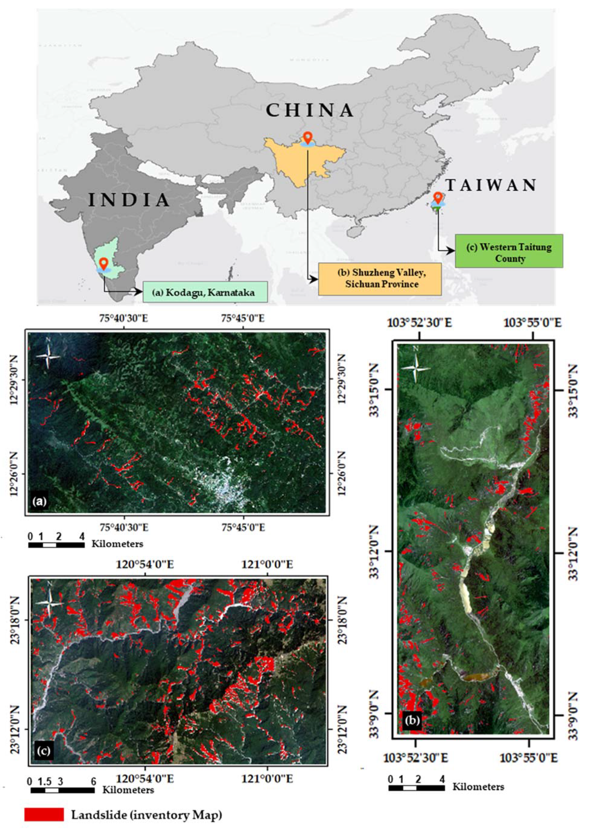
2. Study Areas
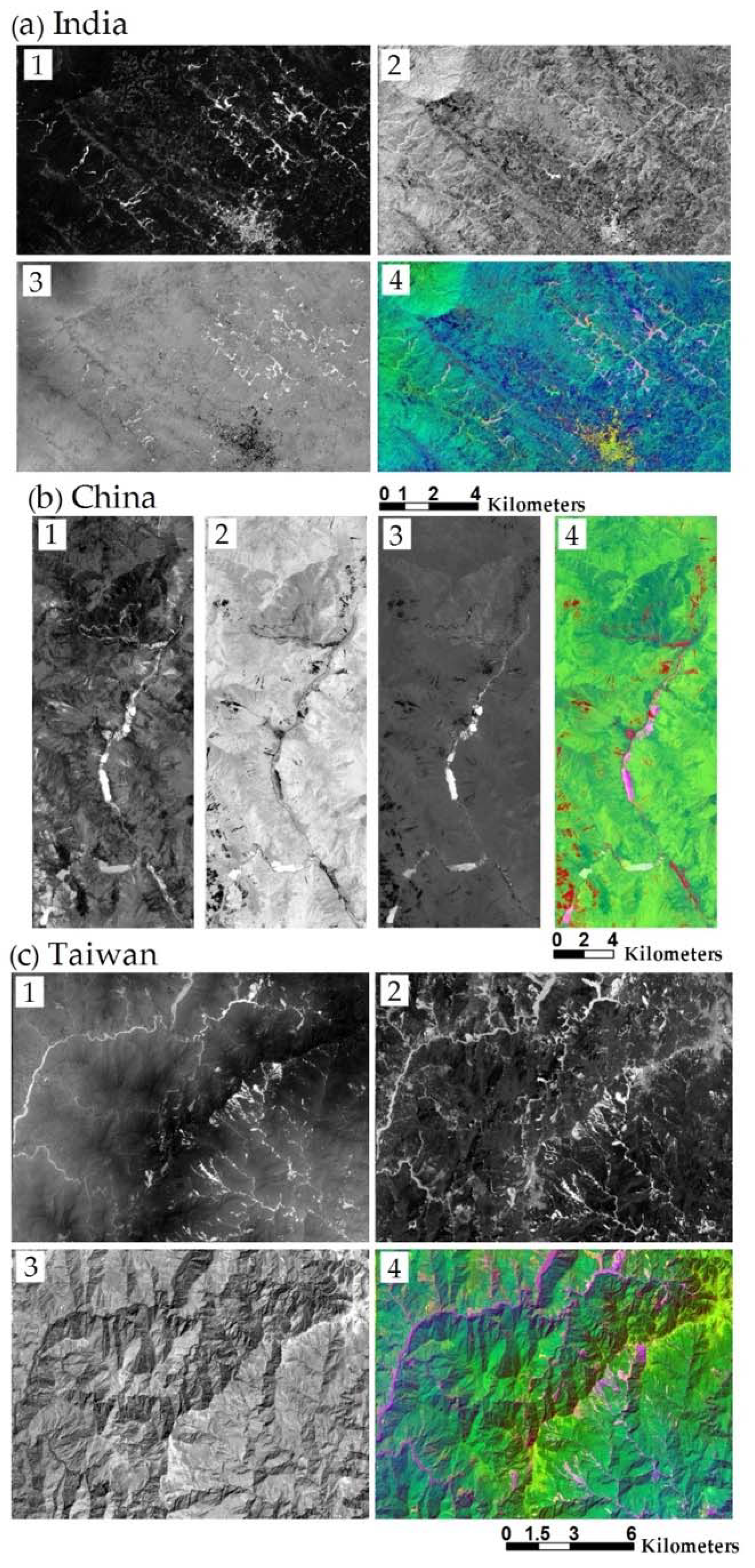
2.1. Kodagu, Karnataka (India)
2.2. Shuzheng Valley, Sichuan Province, (China)
2.3. Western Taitung County (Taiwan)
3. Methodology and Data
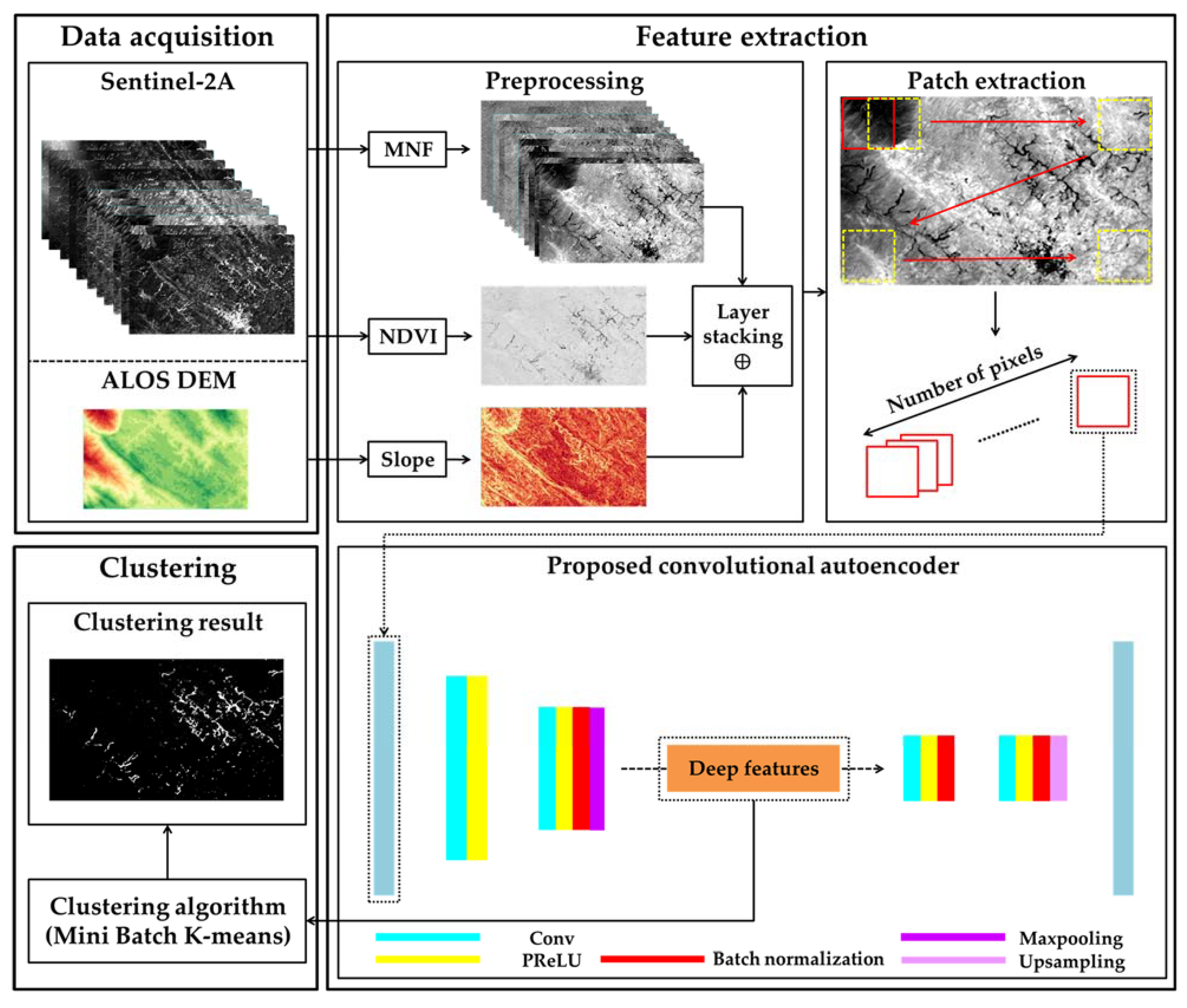
3.1. Overall Workflow
- ▪ Preparing and resampling multispectral images, NDVI, and slope factor;
- ▪ Applying MNF on multispectral images for dimensionality reduction;
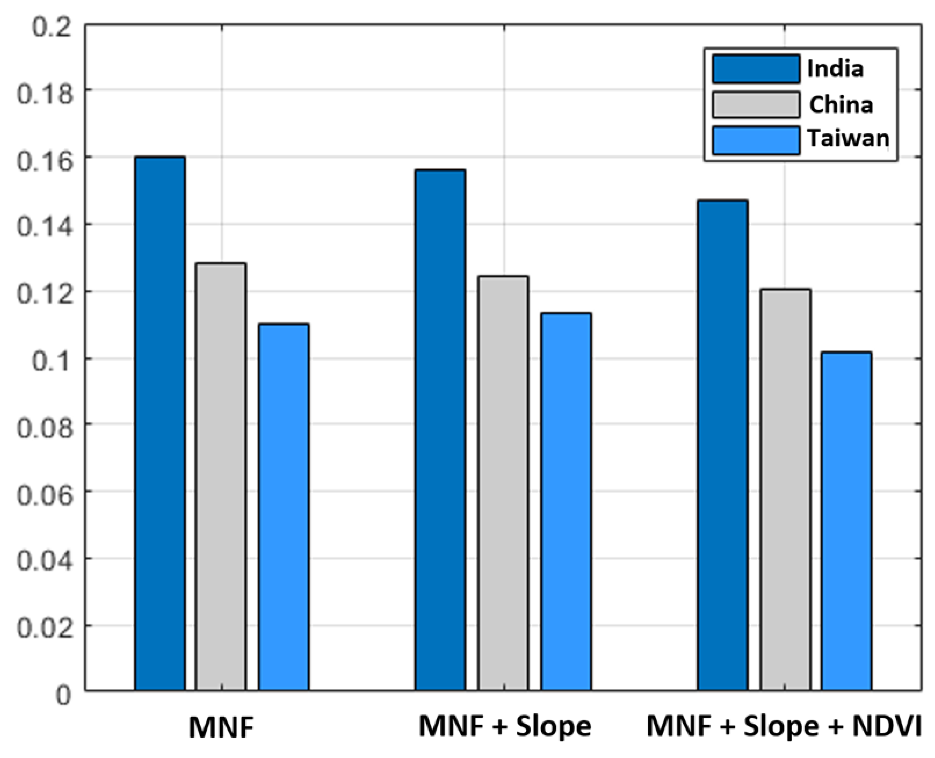
- ▪ Stacking slope factor and NDVI with resulting features from the MNF;
- ▪ Feeding CAE with stacked data;
- ▪ Clustering CAE deep features using mini-batch K-means; and
- ▪ Evaluating clustering results for landslide detection through various accuracy assessment metrics.
3.2. Datasets
3.2.1. Sentinel-2A Data
3.2.2. Landslide Inventory Data
3.2.3. Slope Factor
3.2.4. Normalized Difference Vegetation Index (NDVI)
3.3. Minimum Noise Fraction (MNF) Transformation
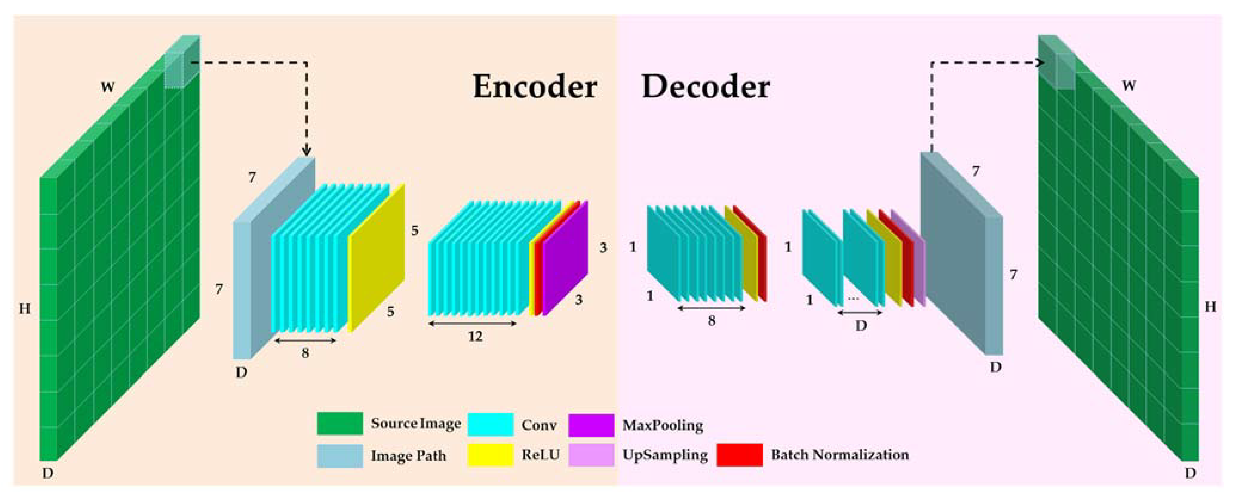
3.4. Convolutional Auto-Encoder (CAE)
3.4.1. Parameter Setting
3.5. Mini-Batch K-Means
4. Results
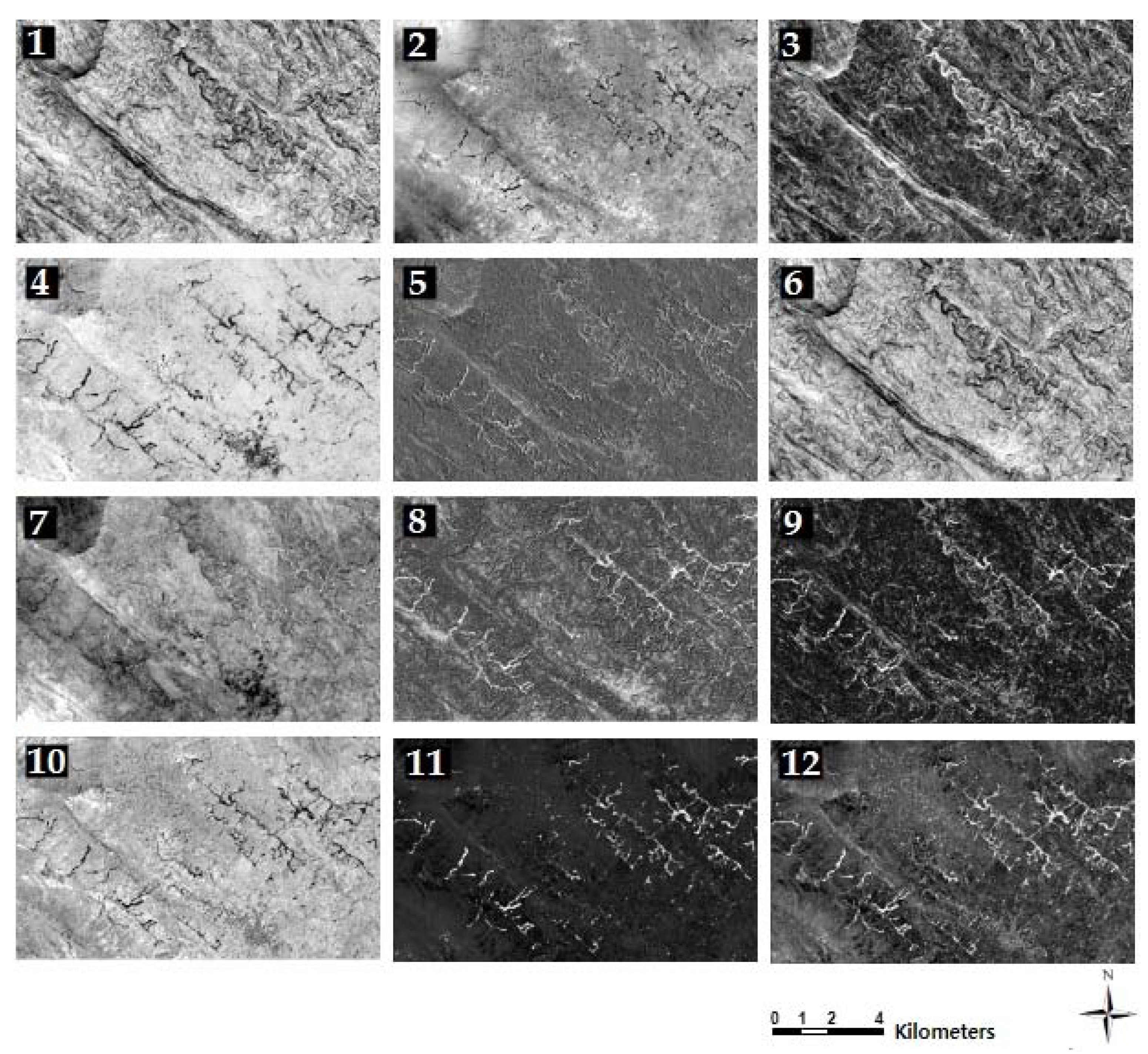
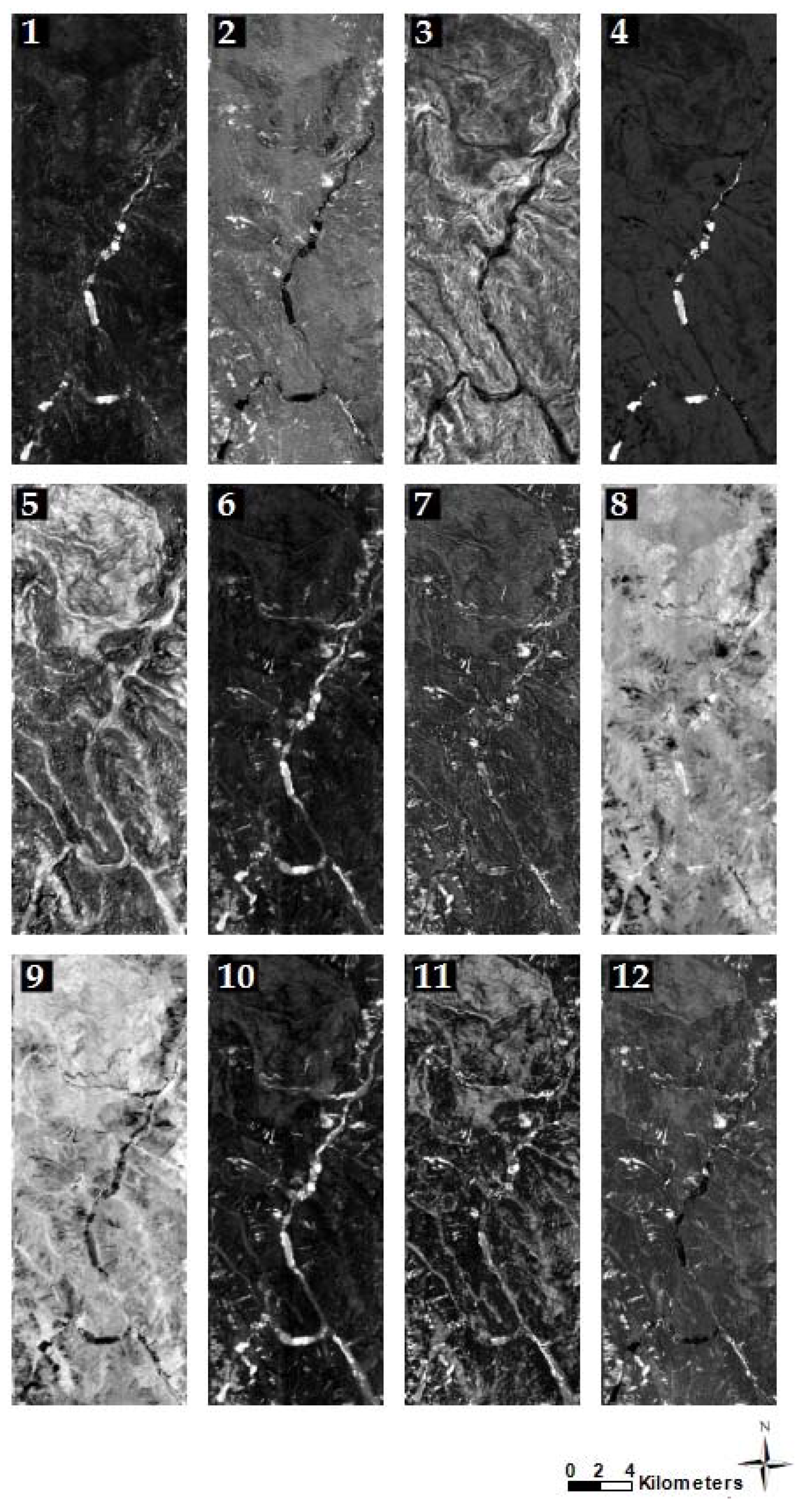
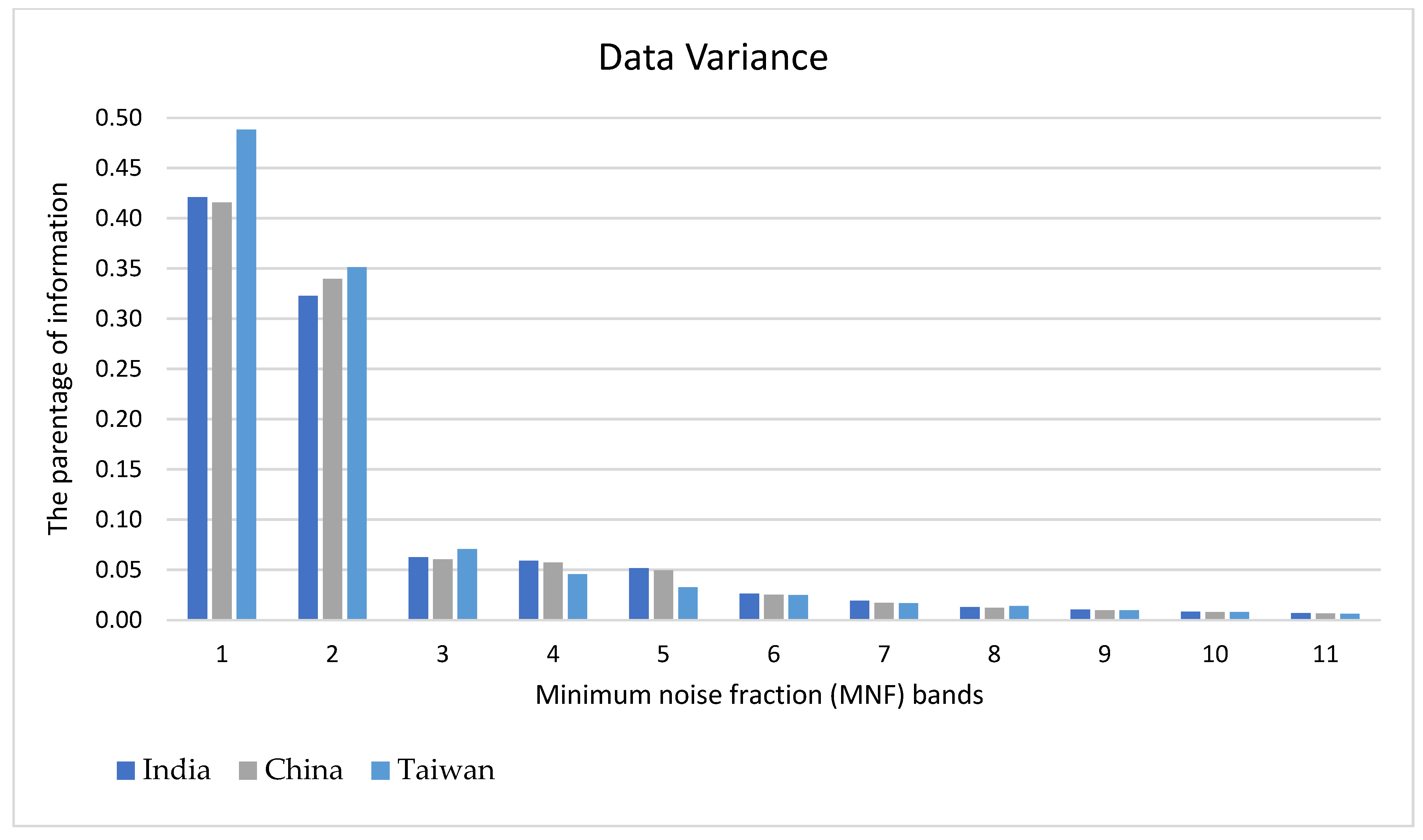
4.1. MNF Transformation
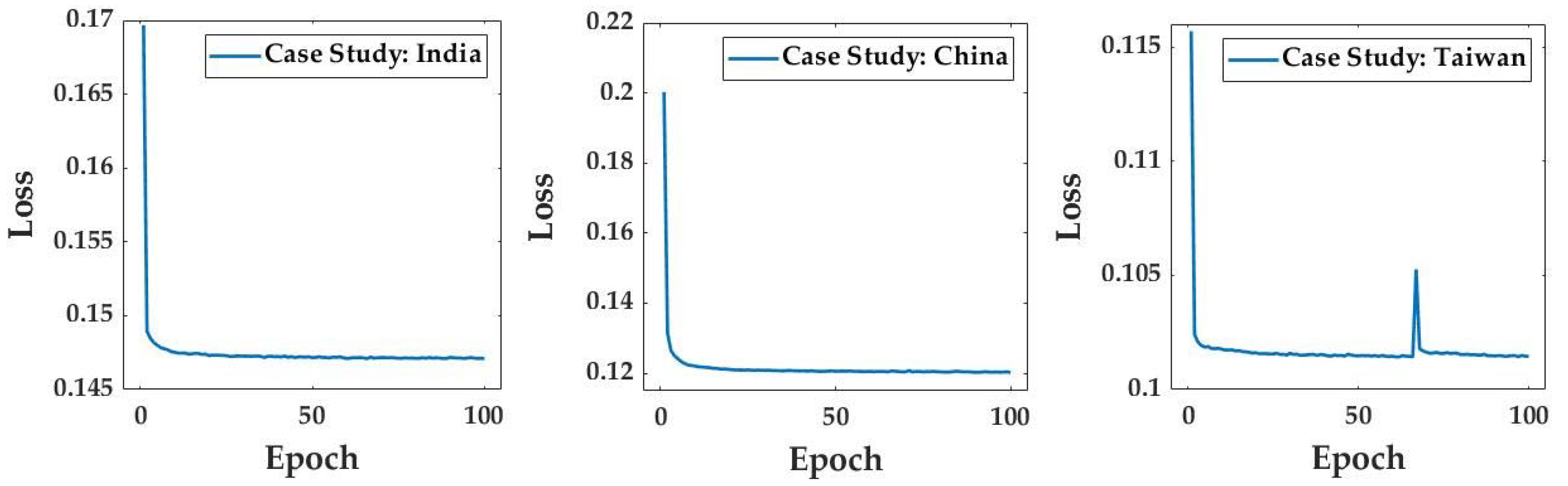
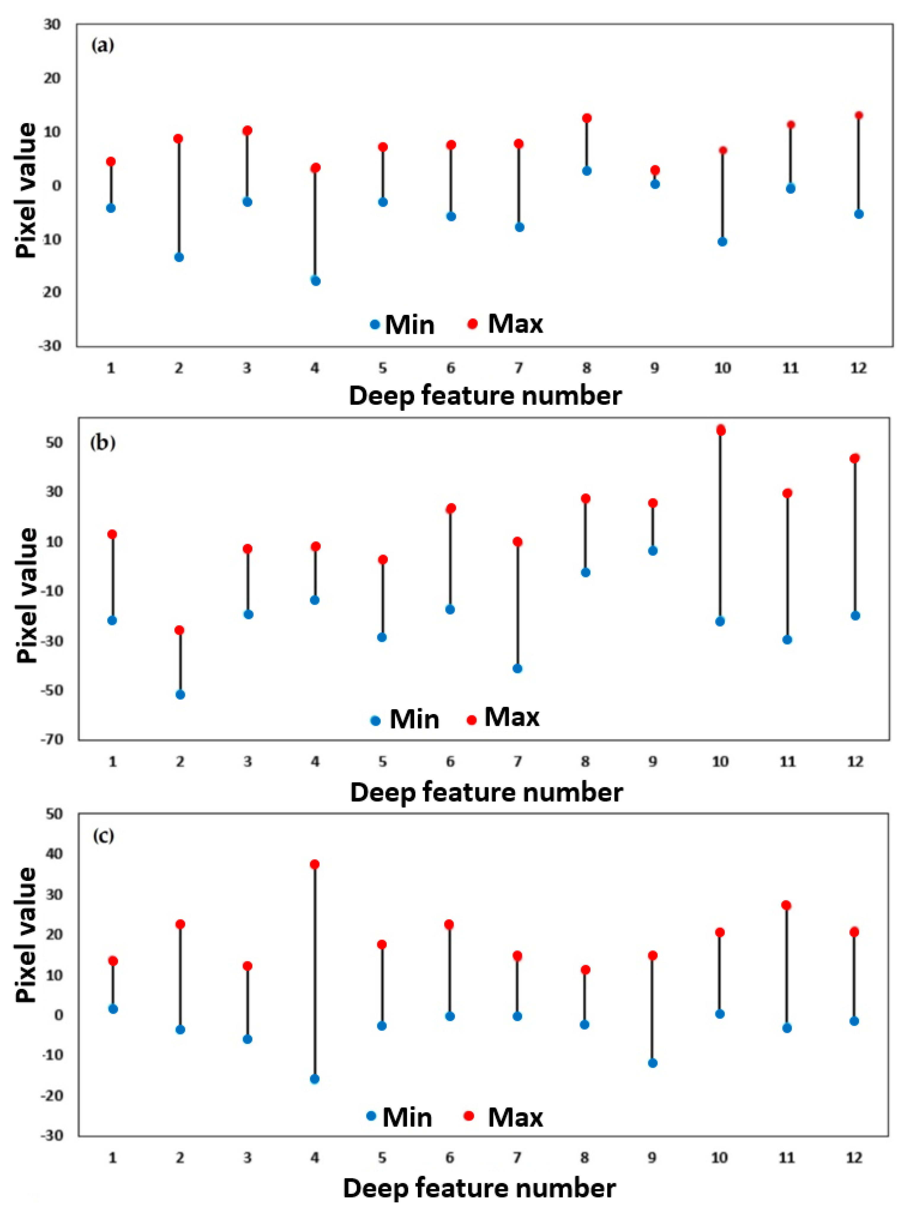
4.2. Experimental Results from the Proposed CAE Model
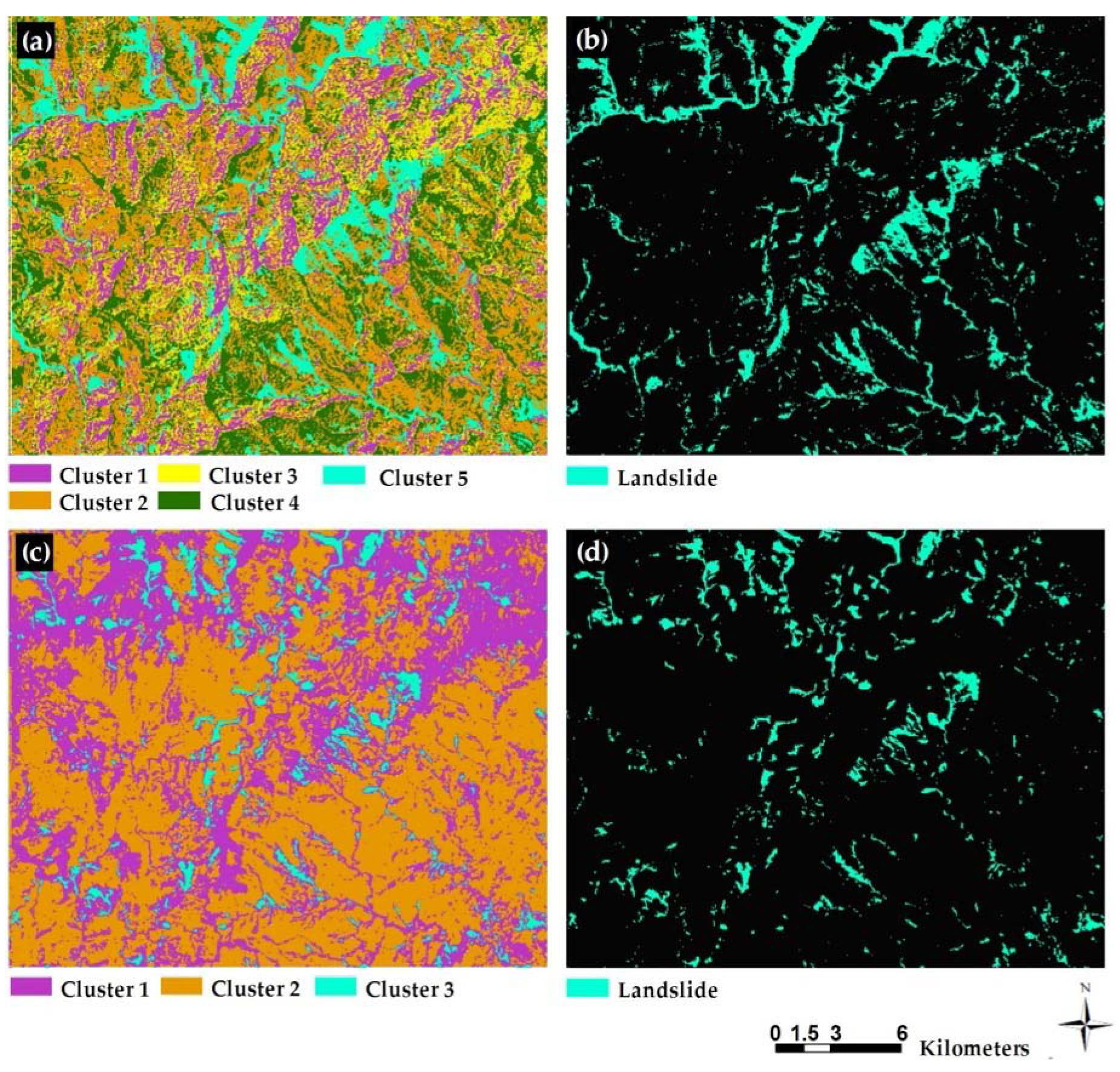
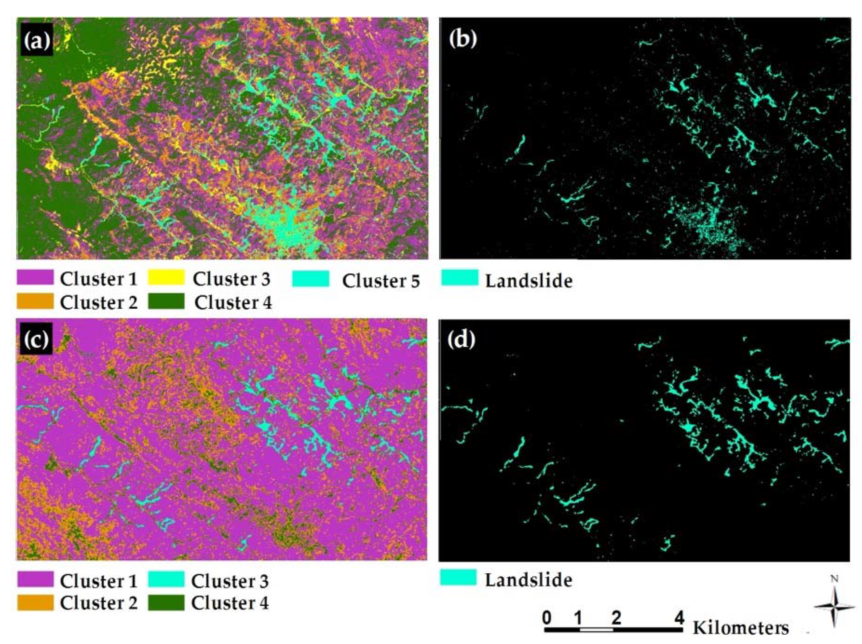
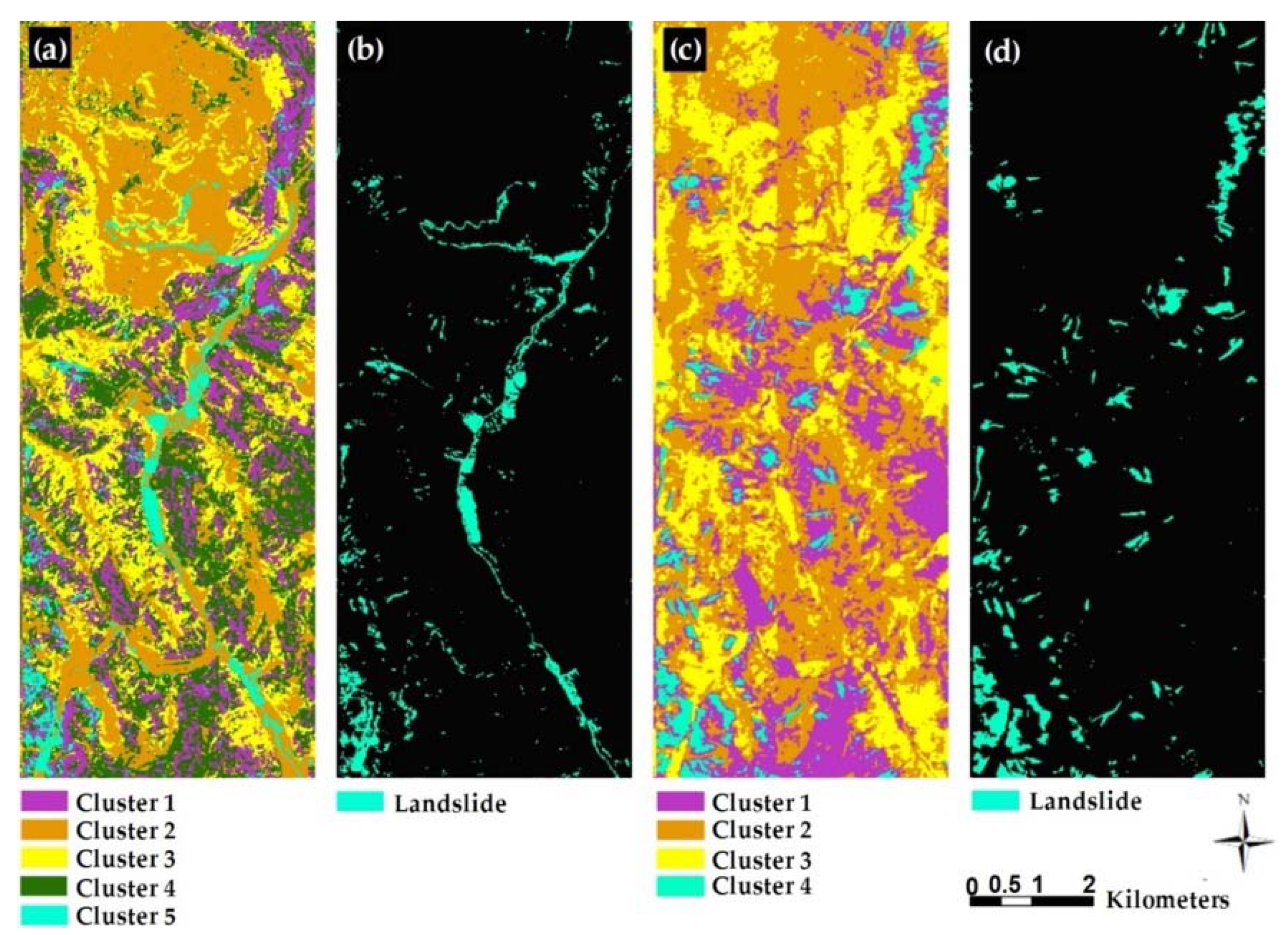
4.3. Clustering Deep Features Using Mini-Batch K-Means
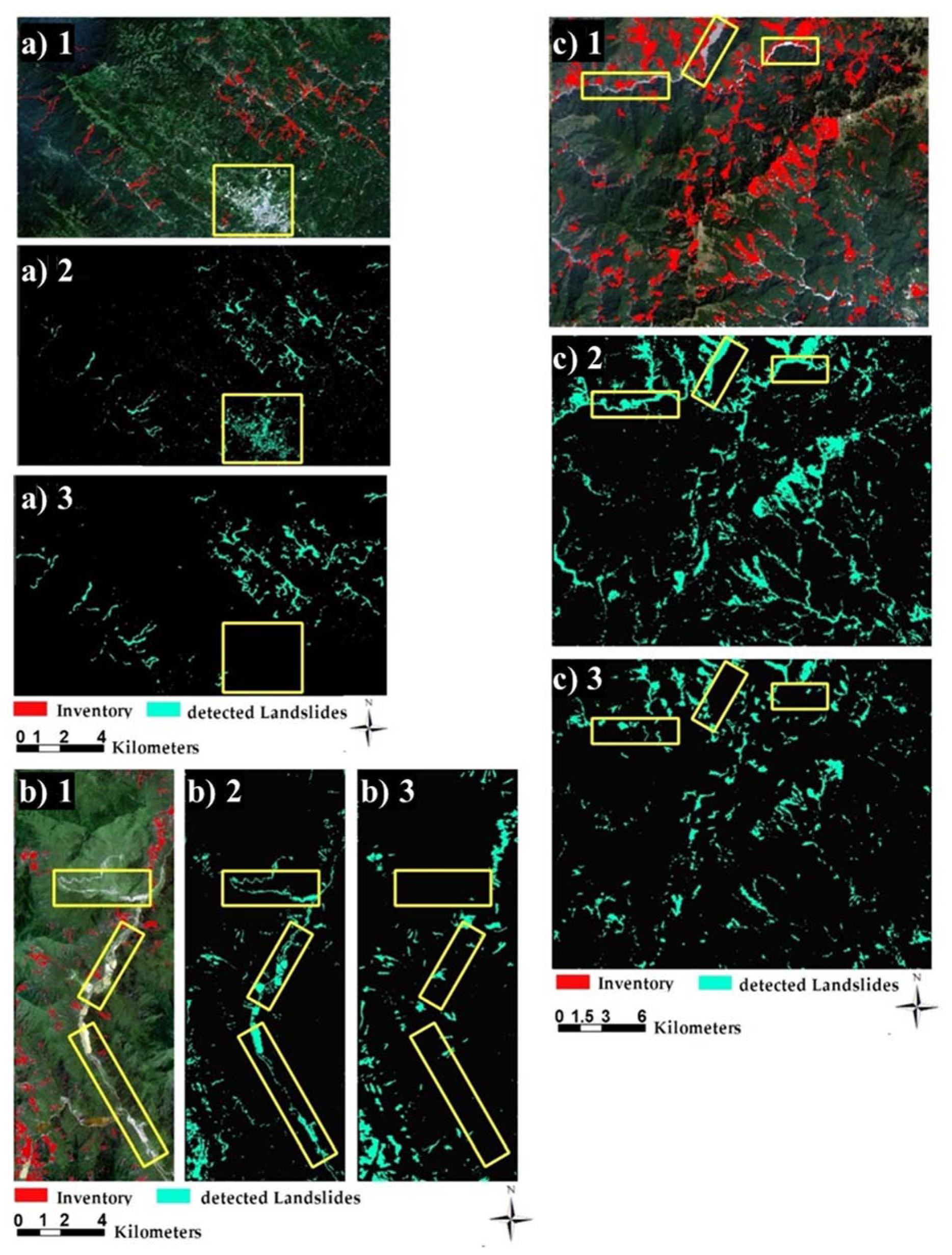
4.4. Accuracy Assessment
5. Discussion
6. Conclusions
Author Contributions
Funding
Institutional Review Board Statement
Informed Consent Statement
Data Availability Statement
Acknowledgments
Conflicts of Interest
References
- Lee, S.; Ryu, J.-H.; Won, J.-S.; Park, H.-J. Determination and application of the weights for landslide susceptibility mapping using an artificial neural network. Eng. Geol. 2004, 71, 289–302. [Google Scholar] [CrossRef]
- Kornejady, A.; Pourghasemi, H.R.; Afzali, S.F. Presentation of RFFR new ensemble model for landslide susceptibility assessment in Iran. In Landslides: Theory, Practice and Modelling; Springer: Berlin/Heidelberg, Germany, 2019; pp. 123–143. [Google Scholar]
- Soares, L.P.; Dias, H.C.; Grohmann, C.H. Landslide Segmentation with U-Net: Evaluating Different Sampling Methods and Patch Sizes. arXiv 2020, arXiv:2007.06672. [Google Scholar]
- Ghorbanzadeh, O.; Blaschke, T.; Gholamnia, K.; Meena, S.R.; Tiede, D.; Aryal, J. Evaluation of Different Machine Learning Methods and Deep-Learning Convolutional Neural Networks for Landslide Detection. Remote Sens. 2019, 11, 196. [Google Scholar] [CrossRef] [Green Version]
- Ambrosi, C.; Strozzi, T.; Scapozza, C.; Wegmüller, U. Landslide hazard assessment in the Himalayas (Nepal and Bhutan) based on Earth-Observation data. Eng. Geol. 2018, 237, 217–228. [Google Scholar] [CrossRef]
- Mondini, A.; Guzzetti, F.; Reichenbach, P.; Rossi, M.; Cardinali, M.; Ardizzone, F. Semi-automatic recognition and mapping of rainfall induced shallow landslides using optical satellite images. Remote Sens. Environ. 2011, 115, 1743–1757. [Google Scholar] [CrossRef]
- Chen, Y.; Wei, Y.; Wang, Q.; Chen, F.; Lu, C.; Lei, S. Mapping Post-Earthquake Landslide Susceptibility: A U-Net Like Approach. Remote Sens. 2020, 12, 2767. [Google Scholar] [CrossRef]
- Chen, W.; Zhang, S.; Li, R.; Shahabi, H. Performance evaluation of the GIS-based data mining techniques of best-first decision tree, random forest, and naïve Bayes tree for landslide susceptibility modeling. Sci. Total Environ. 2018, 644, 1006–1018. [Google Scholar] [CrossRef]
- Dou, J.; Yunus, A.P.; Bui, D.T.; Merghadi, A.; Sahana, M.; Zhu, Z.; Chen, C.-W.; Han, Z.; Pham, B.T. Improved landslide assessment using support vector machine with bagging, boosting, and stacking ensemble machine learning framework in a mountainous watershed, Japan. Landslides 2020, 17, 641–658. [Google Scholar] [CrossRef]
- Tavakkoli Piralilou, S.; Shahabi, H.; Jarihani, B.; Ghorbanzadeh, O.; Blaschke, T.; Gholamnia, K.; Meena, S.R.; Aryal, J. Landslide Detection Using Multi-Scale Image Segmentation and Different Machine Learning Models in the Higher Himalayas. Remote Sens. 2019, 11, 2575. [Google Scholar] [CrossRef] [Green Version]
- Kalantar, B.; Pradhan, B.; Naghibi, S.A.; Motevalli, A.; Mansor, S. Assessment of the effects of training data selection on the landslide susceptibility mapping: A comparison between support vector machine (SVM), logistic regression (LR) and artificial neural networks (ANN). Geomat. Nat. Hazards Risk 2018, 9, 49–69. [Google Scholar] [CrossRef]
- Maxwell, A.E.; Sharma, M.; Kite, J.S.; Donaldson, K.A.; Thompson, J.A.; Bell, M.L.; Maynard, S.M. Slope failure prediction using random forest machine learning and LiDAR in an eroded folded mountain belt. Remote Sens. 2020, 12, 486. [Google Scholar] [CrossRef] [Green Version]
- Yu, B.; Chen, F.; Xu, C.; Wang, L.; Wang, N. Matrix SegNet: A Practical Deep Learning Framework for Landslide Mapping from Images of Different Areas with Different Spatial Resolutions. Remote Sens. 2021, 13, 3158. [Google Scholar] [CrossRef]
- Thi Ngo, P.T.; Panahi, M.; Khosravi, K.; Ghorbanzadeh, O.; Kariminejad, N.; Cerda, A.; Lee, S. Evaluation of deep learning algorithms for national scale landslide susceptibility mapping of Iran. Geosci. Front. 2021, 12, 505–519. [Google Scholar] [CrossRef]
- Tran, C.J.; Mora, O.E.; Fayne, J.V.; Lenzano, M.G. Unsupervised classification for landslide detection from airborne laser scanning. Geosciences 2019, 9, 221. [Google Scholar] [CrossRef] [Green Version]
- Seber, G.A. Multivariate Observations; John Wiley & Sons: Hoboken, NJ, USA, 2009; Volume 252. [Google Scholar]
- Movia, A.; Beinat, A.; Crosilla, F. Shadow detection and removal in RGB VHR images for land use unsupervised classification. ISPRS J. Photogramm. Remote Sens. 2016, 119, 485–495. [Google Scholar] [CrossRef]
- Wang, L.; Sousa, W.P.; Gong, P.; Biging, G.S. Comparison of IKONOS and QuickBird images for mapping mangrove species on the Caribbean coast of Panama. Remote Sens. Environ. 2004, 91, 432–440. [Google Scholar] [CrossRef]
- Solano-Correa, Y.T.; Bovolo, F.; Bruzzone, L. An approach for unsupervised change detection in multitemporal VHR images acquired by different multispectral sensors. Remote Sens. 2018, 10, 533. [Google Scholar] [CrossRef] [Green Version]
- Wan, S.; Chang, S.-H.; Chou, T.-Y.; Shien, C.M. A study of landslide image classification through data clustering using bacterial foraging optimization. J. Chin. Soil Water Conserv. 2018, 49, 187–198. [Google Scholar]
- Abbas, A.W.; Minallh, N.; Ahmad, N.; Abid, S.A.R.; Khan, M.A.A. K-Means and ISODATA clustering algorithms for landcover classification using remote sensing. Sindh Univ. Res. J. Sci. Ser. 2016, 48. Available online: https://sujo-old.usindh.edu.pk/index.php/SURJ/article/view/2358 (accessed on 7 November 2021).
- Ramos-Bernal, R.N.; Vázquez-Jiménez, R.; Romero-Calcerrada, R.; Arrogante-Funes, P.; Novillo, C.J. Evaluation of unsupervised change detection methods applied to landslide inventory mapping using ASTER imagery. Remote Sens. 2018, 10, 1987. [Google Scholar] [CrossRef] [Green Version]
- Mousavi, S.M.; Zhu, W.; Ellsworth, W.; Beroza, G. Unsupervised clustering of seismic signals using deep convolutional autoencoders. IEEE Geosci. Remote Sens. Lett. 2019, 16, 1693–1697. [Google Scholar] [CrossRef]
- Tao, C.; Pan, H.; Li, Y.; Zou, Z. Unsupervised spectral–spatial feature learning with stacked sparse autoencoder for hyperspectral imagery classification. IEEE Geosci. Remote Sens. Lett. 2015, 12, 2438–2442. [Google Scholar]
- Othman, E.; Bazi, Y.; Alajlan, N.; Alhichri, H.; Melgani, F. Using convolutional features and a sparse autoencoder for land-use scene classification. Int. J. Remote Sens. 2016, 37, 2149–2167. [Google Scholar] [CrossRef]
- Ahmad, M.; Khan, A.M.; Mazzara, M.; Distefano, S. Multi-layer Extreme Learning Machine-based Autoencoder for Hyperspectral Image Classification. In Proceedings of the VISIGRAPP (4: VISAPP) 2019, Prague, Czech Republic, 25–27 February 2019; pp. 75–82. [Google Scholar]
- Kalinicheva, E.; Sublime, J.; Trocan, M. Unsupervised Satellite Image Time Series Clustering Using Object-Based Approaches and 3D Convolutional Autoencoder. Remote Sens. 2020, 12, 1816. [Google Scholar] [CrossRef]
- Rahimzad, M.; Homayouni, S.; Alizadeh Naeini, A.; Nadi, S. An Efficient Multi-Sensor Remote Sensing Image Clustering in Urban Areas via Boosted Convolutional Autoencoder (BCAE). Remote Sens. 2021, 13, 2501. [Google Scholar] [CrossRef]
- Rasti, B.; Koirala, B.; Scheunders, P.; Ghamisi, P. Spectral Unmixing Using Deep Convolutional Encoder-Decoder. In Proceedings of the IEEE International Geoscience and Remote Sensing Symposium IGARSS 2021, Brussels, Belgium, 11–16 July 2021; pp. 3829–3832. [Google Scholar]
- Badrinarayanan, V.; Kendall, A.; Cipolla, R. Segnet: A deep convolutional encoder-decoder architecture for image segmentation. IEEE Trans. Pattern Anal. Mach. Intell. 2017, 39, 2481–2495. [Google Scholar] [CrossRef]
- Li, L. Deep Residual Autoencoder with Multiscaling for Semantic Segmentation of Land-Use Images. Remote Sens. 2019, 11, 2142. [Google Scholar] [CrossRef] [Green Version]
- Azarang, A.; Manoochehri, H.E.; Kehtarnavaz, N. Convolutional autoencoder-based multispectral image fusion. IEEE Access 2019, 7, 35673–35683. [Google Scholar] [CrossRef]
- Xu, Y.; Xiang, S.; Huo, C.; Pan, C. Change detection based on auto-encoder model for VHR images. In Proceedings of the MIPPR 2013: Pattern Recognition and Computer Vision, Wuhan, China, 26–27 October 2013; p. 891902. [Google Scholar]
- Lv, N.; Chen, C.; Qiu, T.; Sangaiah, A.K. Deep learning and superpixel feature extraction based on contractive autoencoder for change detection in SAR images. IEEE Trans. Ind. Inform. 2018, 14, 5530–5538. [Google Scholar] [CrossRef]
- Mesquita, D.B.; dos Santos, R.F.; Macharet, D.G.; Campos, M.F.; Nascimento, E.R. Fully Convolutional Siamese Autoencoder for Change Detection in UAV Aerial Images. IEEE Geosci. Remote Sens. Lett. 2019, 17, 1455–1459. [Google Scholar] [CrossRef]
- He, G.; Zhong, J.; Lei, J.; Li, Y.; Xie, W. Hyperspectral Pansharpening Based on Spectral Constrained Adversarial Autoencoder. Remote Sens. 2019, 11, 2691. [Google Scholar] [CrossRef] [Green Version]
- Shao, Z.; Lu, Z.; Ran, M.; Fang, L.; Zhou, J.; Zhang, Y. Residual Encoder-Decoder Conditional Generative Adversarial Network for Pansharpening. IEEE Geosci. Remote Sens. Lett. 2019, 17, 1573–1577. [Google Scholar] [CrossRef]
- Zhao, C.; Li, X.; Zhu, H. Hyperspectral anomaly detection based on stacked denoising autoencoders. J. Appl. Remote Sens. 2017, 11, 042605. [Google Scholar] [CrossRef]
- Chang, S.; Du, B.; Zhang, L. A sparse autoencoder based hyperspectral anomaly detection algorihtm using residual of reconstruction error. In Proceedings of the IGARSS 2019—2019 IEEE International Geoscience and Remote Sensing Symposium, Yokohama, Japan, 28 July–2 August 2019; pp. 5488–5491. [Google Scholar]
- Mukhtar, T.; Khurshid, N.; Taj, M. Dimensionality Reduction Using Discriminative Autoencoders for Remote Sensing Image Retrieval. In Proceedings of the International Conference on Image Analysis and Processing, Trento, Italy, 9–13 September 2019; pp. 499–508. [Google Scholar]
- Song, C.; Liu, F.; Huang, Y.; Wang, L.; Tan, T. Auto-encoder based data clustering. In Proceedings of the Iberoamerican Congress on Pattern Recognition, Havana, Cuba, 20–23 November 2013; pp. 117–124. [Google Scholar]
- Zhang, R.; Yu, L.; Tian, S.; Lv, Y. Unsupervised remote sensing image segmentation based on a dual autoencoder. J. Appl. Remote Sens. 2019, 13, 038501. [Google Scholar] [CrossRef]
- Nalepa, J.; Myller, M.; Imai, Y.; Honda, K.-i.; Takeda, T.; Antoniak, M. Unsupervised segmentation of hyperspectral images using 3-D convolutional autoencoders. IEEE Geosci. Remote Sens. Lett. 2020, 17, 1948–1952. [Google Scholar] [CrossRef]
- Sculley, D. Web-scale k-means clustering. In Proceedings of the 19th International Conference on World Wide Web, Raleigh, NC, USA, 26–30 April 2010; pp. 1177–1178. [Google Scholar]
- Borghuis, A.; Chang, K.; Lee, H. Comparison between automated and manual mapping of typhoon-triggered landslides from SPOT-5 imagery. Int. J. Remote Sens. 2007, 28, 1843–1856. [Google Scholar] [CrossRef]
- Kursa, M.B.; Rudnicki, W.R. Feature selection with the Boruta package. J. Stat. Softw. 2010, 36, 1–13. [Google Scholar] [CrossRef] [Green Version]
- Mezaal, M.R.; Pradhan, B.; Sameen, M.I.; Mohd Shafri, H.Z.; Yusoff, Z.M. Optimized neural architecture for automatic landslide detection from high-resolution airborne laser scanning data. Appl. Sci. 2017, 7, 730. [Google Scholar] [CrossRef] [Green Version]
- Ghorbanzadeh, O.; Meena, S.R.; Abadi, H.S.S.; Piralilou, S.T.; Zhiyong, L.; Blaschke, T. Landslide Mapping Using Two Main Deep-Learning Convolution Neural Network (CNN) Streams Combined by the Dempster—Shafer (DS) model. IEEE J. Sel. Top. Appl. Earth Obs. Remote Sens. 2020, 14, 452–463. [Google Scholar] [CrossRef]
- Stumpf, A.; Kerle, N. Object-oriented mapping of landslides using Random Forests. Remote Sens. Environ. 2011, 115, 2564–2577. [Google Scholar] [CrossRef]
- Su, Z.; Chow, J.K.; Tan, P.S.; Wu, J.; Ho, Y.K.; Wang, Y.-H. Deep convolutional neural network–based pixel-wise landslide inventory mapping. Landslides 2020, 18, 1421–1443. [Google Scholar] [CrossRef]
- Sachin Kumar, M.; Gurav, M.; Kushalappa, C.; Vaast, P. Spatial and temporal changes in rainfall patterns in coffee landscape of Kodagu, India. Int. J. Environ. Sci. 2012, 1, 168–172. [Google Scholar]
- Shreyas, R.; Punith, D.; Bhagirathi, L.; Krishna, A.; Devagiri, G. Exploring Different Probability Distributions for Rainfall Data of Kodagu-An Assisting Approach for Food Security. Int. J. Curr. Microbiol. Appl. Sci. 2020, 9, 2972–2980. [Google Scholar] [CrossRef]
- Thomas, J.J.; Prakash, B.; Kulkarni, P.; MR, N.M. Exploring the psychiatric symptoms among people residing at flood affected areas of Kodagu district, Karnataka. Clin. Epidemiol. Glob. Health 2020, 9, 245–250. [Google Scholar] [CrossRef]
- Hu, X.; Hu, K.; Tang, J.; You, Y.; Wu, C. Assessment of debris-flow potential dangers in the Jiuzhaigou Valley following the August 8, 2017, Jiuzhaigou earthquake, western China. Eng. Geol. 2019, 256, 57–66. [Google Scholar] [CrossRef]
- Zhao, B.; Wang, Y.-S.; Luo, Y.-H.; Li, J.; Zhang, X.; Shen, T. Landslides and dam damage resulting from the Jiuzhaigou earthquake (August 8 2017), Sichuan, China. R. Soc. Open Sci. 2018, 5, 171418. [Google Scholar] [CrossRef] [PubMed] [Green Version]
- Lin, C.-W.; Chang, W.-S.; Liu, S.-H.; Tsai, T.-T.; Lee, S.-P.; Tsang, Y.-C.; Shieh, C.-L.; Tseng, C.-M. Landslides triggered by the August 7 2009 Typhoon Morakot in southern Taiwan. Eng. Geol. 2011, 123, 3–12. [Google Scholar] [CrossRef]
- Lin, C.-W.; Tseng, C.-M.; Tseng, Y.-H.; Fei, L.-Y.; Hsieh, Y.-C.; Tarolli, P. Recognition of large scale deep-seated landslides in forest areas of Taiwan using high resolution topography. J. Asian Earth Sci. 2013, 62, 389–400. [Google Scholar] [CrossRef]
- Sentinel, E. User Handbook; ESA Standard Document 64; ESA: Darmstadt, Germany, 2015. [Google Scholar]
- Main-Knorn, M.; Pflug, B.; Louis, J.; Debaecker, V.; Müller-Wilm, U.; Gascon, F. Sen2Cor for sentinel-2. In Proceedings of the Image and Signal Processing for Remote Sensing XXIII, Warsaw, Poland, 11–13 September 2017; p. 1042704. [Google Scholar]
- Poursanidis, D.; Traganos, D.; Reinartz, P.; Chrysoulakis, N. On the use of Sentinel-2 for coastal habitat mapping and satellite-derived bathymetry estimation using downscaled coastal aerosol band. Int. J. Appl. Earth Obs. Geoinf. 2019, 80, 58–70. [Google Scholar] [CrossRef]
- Makarau, A.; Richter, R.; Schläpfer, D.; Reinartz, P. APDA water vapor retrieval validation for Sentinel-2 imagery. IEEE Geosci. Remote Sens. Lett. 2016, 14, 227–231. [Google Scholar] [CrossRef] [Green Version]
- Team, P. Planet Imagery Product Specifications; Planet Team: San Francisco, CA, USA, 2018. [Google Scholar]
- Nhu, V.-H.; Mohammadi, A.; Shahabi, H.; Ahmad, B.B.; Al-Ansari, N.; Shirzadi, A.; Geertsema, M.; Kress, V.R.; Karimzadeh, S.; Valizadeh Kamran, K. Landslide Detection and Susceptibility Modeling on Cameron Highlands (Malaysia): A Comparison between Random Forest, Logistic Regression and Logistic Model Tree Algorithms. Forests 2020, 11, 830. [Google Scholar] [CrossRef]
- Pourghasemi, H.R.; Rahmati, O. Prediction of the landslide susceptibility: Which algorithm, which precision? Catena 2018, 162, 177–192. [Google Scholar] [CrossRef]
- ASF DAAC. ALOS PALSAR_Radiometric_Terrain_Corrected_low_res. Includes Material© JAXA/METI 2007. Available online: https://asf.alaska.edu:2015 (accessed on 7 November 2021).
- Pettorelli, N. The Normalized Difference Vegetation Index; Oxford University Press: Oxford, UK, 2013. [Google Scholar]
- Cihlar, J.; Laurent, L.S.; Dyer, J. Relation between the normalized difference vegetation index and ecological variables. Remote Sens. Environ. 1991, 35, 279–298. [Google Scholar] [CrossRef]
- Green, A.A.; Berman, M.; Switzer, P.; Craig, M.D. A transformation for ordering multispectral data in terms of image quality with implications for noise removal. IEEE Trans. Geosci. Remote Sens. 1988, 26, 65–74. [Google Scholar] [CrossRef] [Green Version]
- Ghorbanzadeh, O.; Dabiri, Z.; Tiede, D.; Piralilo, S.T.; Blaschke, T.; Lang, S. Evaluation of Minimum Noise Fraction Transformation and Independent Component Analysis for Dwelling Annotation in Refugee Camps Using Convolutional Neural Network. In Proceedings of the 39th Annual EARSeL Symposium, Salzurg, Austria, 1–4 July 2019. [Google Scholar]
- Luo, G.; Chen, G.; Tian, L.; Qin, K.; Qian, S.-E. Minimum noise fraction versus principal component analysis as a pre-processing step for hyperspectral imagery denoising. Can. J. Remote Sens. 2016, 42, 106–116. [Google Scholar] [CrossRef]
- Yang, M.-D.; Huang, K.-H.; Tsai, H.-P. Integrating MNF and HHT Transformations into Artificial Neural Networks for Hyperspectral Image Classification. Remote Sens. 2020, 12, 2327. [Google Scholar] [CrossRef]
- Lixin, G.; Weixin, X.; Jihong, P. Segmented minimum noise fraction transformation for efficient feature extraction of hyperspectral images. Pattern Recognit. 2015, 48, 3216–3226. [Google Scholar] [CrossRef]
- Affeldt, S.; Labiod, L.; Nadif, M. Spectral clustering via ensemble deep autoencoder learning (SC-EDAE). Pattern Recognit. 2020, 108, 107522. [Google Scholar] [CrossRef]
- Min, E.; Guo, X.; Liu, Q.; Zhang, G.; Cui, J.; Long, J. A survey of clustering with deep learning: From the perspective of network architecture. IEEE Access 2018, 6, 39501–39514. [Google Scholar] [CrossRef]
- Vincent, P.; Larochelle, H.; Lajoie, I.; Bengio, Y.; Manzagol, P.-A.; Bottou, L. Stacked denoising autoencoders: Learning useful representations in a deep network with a local denoising criterion. J. Mach. Learn. Res. 2010, 11, 3371–3408. [Google Scholar]
- Tang, X.; Zhang, X.; Liu, F.; Jiao, L. Unsupervised deep feature learning for remote sensing image retrieval. Remote Sens. 2018, 10, 1243. [Google Scholar] [CrossRef] [Green Version]
- Tharani, M.; Khurshid, N.; Taj, M. Unsupervised deep features for remote sensing image matching via discriminator network. arXiv 2018, arXiv:1810.06470. [Google Scholar]
- Li, F.; Qiao, H.; Zhang, B. Discriminatively boosted image clustering with fully convolutional auto-encoders. Pattern Recognit. 2018, 83, 161–173. [Google Scholar] [CrossRef] [Green Version]
- Ribeiro, M.; Lazzaretti, A.E.; Lopes, H.S. A study of deep convolutional auto-encoders for anomaly detection in videos. Pattern Recognit. Lett. 2018, 105, 13–22. [Google Scholar] [CrossRef]
- Zhao, W.; Guo, Z.; Yue, J.; Zhang, X.; Luo, L. On combining multiscale deep learning features for the classification of hyperspectral remote sensing imagery. Int. J. Remote Sens. 2015, 36, 3368–3379. [Google Scholar] [CrossRef]
- Masci, J.; Meier, U.; Cireşan, D.; Schmidhuber, J. Stacked convolutional auto-encoders for hierarchical feature extraction. In Proceedings of the International Conference on Artificial Neural Networks, Espoo, Finland, 14–17 June 2011; pp. 52–59. [Google Scholar]
- Ioffe, S.; Szegedy, C. Batch normalization: Accelerating deep network training by reducing internal covariate shift. arXiv 2015, arXiv:1502.03167. [Google Scholar]
- Song, C.; Huang, Y.; Liu, F.; Wang, Z.; Wang, L. Deep auto-encoder based clustering. Intell. Data Anal. 2014, 18, S65–S76. [Google Scholar] [CrossRef]
- Chen, Y.; Wang, Y.; Gu, Y.; He, X.; Ghamisi, P.; Jia, X. Deep learning ensemble for hyperspectral image classification. IEEE J. Sel. Top. Appl. Earth Obs. Remote Sens. 2019, 12, 1882–1897. [Google Scholar] [CrossRef]
- Khan, S.; Rahmani, H.; Shah, S.A.A.; Bennamoun, M. A guide to convolutional neural networks for computer vision. Synth. Lect. Comput. Vis. 2018, 8, 1–207. [Google Scholar] [CrossRef]
- Xiao, B.; Wang, Z.; Liu, Q.; Liu, X. SMK-means: An improved mini batch k-means algorithm based on mapreduce with big data. Comput. Mater. Contin. 2018, 56, 365–379. [Google Scholar]
- O’Malley, T.; Bursztein, E.; Long, J.; Chollet, F.; Jin, H.; Invernizzi, L. Keras Tuner. 2020. Available online: https://keras.io/keras_tuner/ (accessed on 7 November 2021).
- Lobry, S.; Tuia, D. Deep learning models to count buildings in high-resolution overhead images. In Proceedings of the 2019 Joint Urban Remote Sensing Event (JURSE), Vannes, France, 22–24 May 2019; pp. 1–4. [Google Scholar]
- Shahabi, H.; Jarihani, B.; Tavakkoli Piralilou, S.; Chittleborough, D.; Avand, M.; Ghorbanzadeh, O. A Semi-Automated Object-Based Gully Networks Detection Using Different Machine Learning Models: A Case Study of Bowen Catchment, Queensland, Australia. Sensors 2019, 19, 4893. [Google Scholar] [CrossRef] [PubMed] [Green Version]
- Barbu, M.; Radoi, A.; Suciu, G. Landslide Monitoring using Convolutional Autoencoders. In Proceedings of the 2020 12th International Conference on Electronics, Computers and Artificial Intelligence (ECAI), Bucharest, Romania, 25–27 June 2020; pp. 1–6. [Google Scholar]


| Study Area | Number of Landslides | Length (m) | Slope (Degree) | Area (ha) | Total Area (ha) | ||||||
|---|---|---|---|---|---|---|---|---|---|---|---|
| Min | Max | Average | Min | Max | Average | Min | Max | Average | |||
| India | 212 | 45 | 1108 | 870 | 5 | 33 | 17 | 1.7 | 12.4 | 6.1 | 578.60 |
| China | 220 | 120 | 1050 | 724 | 12 | 51 | 42 | 0.8 | 9.5 | 6.3 | 274.47 |
| Taiwan | 720 | 90 | 990 | 720 | 16 | 46 | 32 | 0.45 | 7.1 | 3.1 | 2470.9 |
| Section | Unit | Input Shape | Kernel Size | Output Shape |
|---|---|---|---|---|
| Encoder | CNN1 + PReLU | |||
| CNN2 + PReLU + BN | ||||
| MaxPooling | ||||
| Decoder | CNN3 + PReLU + BN | |||
| CNN4 + PReLU + BN | ||||
| UpSampling |
| MNF Band | India | China | Taiwan | ||||||
|---|---|---|---|---|---|---|---|---|---|
| Eigenvalue | Data Variance | Eigenvalue | Data Variance | Eigenvalue | Data Variance | ||||
| Per Band | Cumulative | Per Band | Cumulative | Per Band | Cumulative | ||||
| 1 | 91.78 | 0.42 | 0.42 | 88.53 | 0.42 | 0.42 | 95.76 | 0.49 | 0.42 |
| 2 | 70.41 | 0.32 | 0.74 | 72.10 | 0.34 | 0.76 | 78.10 | 0.35 | 0.77 |
| 3 | 13.59 | 0.06 | 0.81 | 12.04 | 0.06 | 0.82 | 15.33 | 0.07 | 0.84 |
| 4 | 12.85 | 0.06 | 0.87 | 11.05 | 0.06 | 0.87 | 9.85 | 0.05 | 0.89 |
| 5 | 11.25 | 0.05 | 0.92 | 9.68 | 0.05 | 0.92 | 8.41 | 0.03 | 0.92 |
| 6 | 5.69 | 0.03 | 0.94 | 6.89 | 0.03 | 0.95 | 6.02 | 0.02 | 0.95 |
| 7 | 4.15 | 0.02 | 0.96 | 3.57 | 0.02 | 0.96 | 4.01 | 0.02 | 0.96 |
| 8 | 2.81 | 0.01 | 0.97 | 2.42 | 0.01 | 0.98 | 2.72 | 0.01 | 0.98 |
| 9 | 2.23 | 0.01 | 0.98 | 1.92 | 0.01 | 0.99 | 2.16 | 0.01 | 0.99 |
| 10 | 1.80 | 0.01 | 0.99 | 1.55 | 0.01 | 0.99 | 1.74 | 0.01 | 0.99 |
| 11 | 1.51 | 0.01 | 1.00 | 1.30 | 0.01 | 1.00 | 1.46 | 0.01 | 1.00 |
| Case Study | Clustering with | TP (ha) | FP (ha) | FN (ha) | Precision % | Recall % | F1-Measure % | mIOU % |
|---|---|---|---|---|---|---|---|---|
| India | MNF, Slope, and NDVI | 422.00 | 1063.40 | 156.60 | 28.00 | 73.00 | 41.00 | 26.00 |
| Deep Features | 526.50 | 169.80 | 52.10 | 76.00 | 91.00 | 83.00 | 70.00 | |
| China | MNF, Slope, and NDVI | 93.67 | 121.07 | 181.07 | 0.44 | 0.34 | 0.38 | 0.24 |
| Deep Features | 239.37 | 94.94 | 35.37 | 0.72 | 0.87 | 0.79 | 0.60 | |
| Taiwan | MNF, Slope, and NDVI | 1718.50 | 1247.36 | 752.40 | 0.58 | 0.70 | 0.63 | 0.50 |
| Deep Features | 2014.00 | 599.50 | 456.91 | 0.77 | 0.82 | 0.79 | 0.81 |
Publisher’s Note: MDPI stays neutral with regard to jurisdictional claims in published maps and institutional affiliations. |
© 2021 by the authors. Licensee MDPI, Basel, Switzerland. This article is an open access article distributed under the terms and conditions of the Creative Commons Attribution (CC BY) license (https://creativecommons.org/licenses/by/4.0/).
Share and Cite
Shahabi, H.; Rahimzad, M.; Tavakkoli Piralilou, S.; Ghorbanzadeh, O.; Homayouni, S.; Blaschke, T.; Lim, S.; Ghamisi, P. Unsupervised Deep Learning for Landslide Detection from Multispectral Sentinel-2 Imagery. Remote Sens. 2021, 13, 4698. https://doi.org/10.3390/rs13224698
Shahabi H, Rahimzad M, Tavakkoli Piralilou S, Ghorbanzadeh O, Homayouni S, Blaschke T, Lim S, Ghamisi P. Unsupervised Deep Learning for Landslide Detection from Multispectral Sentinel-2 Imagery. Remote Sensing. 2021; 13(22):4698. https://doi.org/10.3390/rs13224698
Chicago/Turabian StyleShahabi, Hejar, Maryam Rahimzad, Sepideh Tavakkoli Piralilou, Omid Ghorbanzadeh, Saied Homayouni, Thomas Blaschke, Samsung Lim, and Pedram Ghamisi. 2021. "Unsupervised Deep Learning for Landslide Detection from Multispectral Sentinel-2 Imagery" Remote Sensing 13, no. 22: 4698. https://doi.org/10.3390/rs13224698
APA StyleShahabi, H., Rahimzad, M., Tavakkoli Piralilou, S., Ghorbanzadeh, O., Homayouni, S., Blaschke, T., Lim, S., & Ghamisi, P. (2021). Unsupervised Deep Learning for Landslide Detection from Multispectral Sentinel-2 Imagery. Remote Sensing, 13(22), 4698. https://doi.org/10.3390/rs13224698