Modeling Vegetation Water Stress over the Forest from Space: Temperature Vegetation Water Stress Index (TVWSI)

Abstract

The conventional Land Surface Temperature (LST)–Normalized Difference Vegetation Index (NDVI) trapezoid model has been widely used to retrieve vegetation water stress. However, it has two inherent limitations: (1) its complex and computationally intensive parameterization for multi-temporal observations and (2) deficiency in canopy water content information. We tested the hypothesis that an improved water stress index could be constructed by the representation of canopy water content information to the LST–NDVI trapezoid model. Therefore, this study proposes a new index that combines three indicators associated with vegetation water stress: canopy temperature through LST, canopy water content through Surface Water Content Index (SWCI), and canopy fractional cover through NDVI in one temporally transferrable index. Firstly, a new optical space of SWCI–NDVI was conceptualized based on the linear physical relationship between shortwave infrared (SWIR) and soil moisture. Secondly, the SWCI–NDVI feature space was parameterized, and an index d(SWCI, NDVI) was computed based on the distribution of the observations in the SWCI–NDVI spectral space. Finally, standardized LST (LST/long term mean of LST) was combined to d(SWCI, NDVI) to give a new water stress index, Temperature Vegetation Water Stress Index (TVWSI). The modeled soil moisture from the Australian Water Resource Assessment—Landscape (AWRA-L) and Soil Water Fraction (SWF) from four FLUXNET sites across Victoria and New South Wales were used to evaluate TVWSI. The index TVWSI exhibited a high correlation with AWRA-L soil moisture (R² of 0.71 with p < 0.001) and the ground-based SWF (R² of 0.25–0.51 with p < 0.001). TVWSI predicted soil moisture more accurately with RMSE of 21.82 mm (AWRA-L) and 0.02–0.04 (SWF) compared to the RMSE ranging 28.98–36.68 mm (AWRA-L) and 0.03–0.05 (SWF) were obtained for some widely used water stress indices. The TVWSI could also be a useful input parameter for other environmental models.

1. Introduction

Large variations in rainfall and temperature may push forests into a non-recoverable stage of water stress [1,2,3]. In Australia, several studies documented the severe effects of long droughts or heat waves on the ecosystem in the form of canopy decline and mortality [4,5,6,7,8,9].

Eucalypts are the dominant forest type in Australia. Although many eucalypt species are adapted to seasonal water limitation, extreme droughts impose water stress in many areas, and hot summers can cause seasonal water deficits in non-drought years. Vegetation water stress is a significant factor when defining ecosystem-level health and has been used as a critical indicator of environmental quality [10,11]. This indicator can vary significantly over a few hectares, making field-based environmental surveillance of tree water stress a costly and logistically impractical task [12,13]. Remote sensing techniques can map spatio-temporal variations in water stress in forested landscapes. In particular, optical and thermal remotely sensed satellite sensor data were used to develop water stress indices.

Spectral space relations derived from the Land Surface Temperature–Vegetation Index (LST–VI) are based on the nominal links between soil moisture and plant biophysical characteristics [14,15,16,17,18,19]. Most studies found that LST–VI has direct and “instant” links with water stress measures due to the relatively immediate stomatal response to water stress detected by canopy temperature variations. The literature suggests that LST–VI-based methods can readily capture water stress signals without requiring ancillary rainfall data and soil hydraulic properties [20].

Strong negative relationships between LST and VI were reported by many studies, mainly in the water-limited summer season [16,21,22,23,24,25,26]. This negative relation is expressed as a trapezoidal relationship. The trapezoidal relation of LST–NDVI was initially developed by Goward and Hope [27] and subsequently by Moran et al. [16] and Price [28]. The ensuing research has used this feature space to analyze vegetation water stress status and surface soil moisture estimation [15,17,18,19,29,30,31,32,33,34]. Various indices are devised from the LST–VI spectral space based on a simple semi-empirical approach to derive evapotranspiration (ET)-related quantities. Some of the widely accepted indices include: LST–VI slope based indices [23,24,25], Temperature Vegetation Dryness Index (TVDI) [18], Vegetation Water Supply Index (VWSI) [21,35,36], Modified Vegetation Water Supply Index (MVWSI) [37], Vegetation Temperature Condition Index (VTCI) [29,38], Temperature Vegetation Soil Moisture Dryness Index (TVMDI) [15], Temperature Condition Index (TCI), Vegetation Health Index (VHI) [39,40], and LST/NDVI ratio [41].

The relative value of ET-related quantities such as surface soil water content and surface energy fluxes can be defined by pixel position within the LST–NDVI trapezoid. Although the pixel position is influenced by several factors such as vegetation cover, surface roughness, net radiation, and surface thermal property, the dominant influence usually comes from changes in ET due to plant-available soil moisture [18]. As shown in Figure 1, the pixels representing dense vegetation with non-limiting soil moisture sit towards the lower right edge of the trapezoid while pixels from bare, dry soil cluster at the upper edge of the trapezoid. A transition from dense wet vegetation to bare, dry soil can be conceptualized by moving along the dry edge of the triangle (Figure 1). Suppose the NDVI (x-axis) range is divided into bins. In that case, the variation in the LST (y-axis) of vegetation pixels under an NDVI bin could be related to the water stress stages of the vegetation represented by the pixel. The pixels with relatively high LST among other pixels within a bin of NDVI generally represent water-stressed pixels.

Despite the wide acceptance of the LST–NDVI feature space in estimating soil moisture, it has some limitations. Improvements in parameterization were proposed to enhance LST–NDVI capability. For example, Rahimzadeh-Bajgiran et al. [17] considered a non-linear relationship between LST and soil moisture content rather than considering it linear, which was the original concept of LST–NDVI. Sun [42] proposed a two-stage trapezoid because the LST of a vegetative surface is less responsive to surface soil moisture than the bare surface, as trees can extract deep soil water, making the LST–soil moisture relationship non-linear. Tao et al. [43] identified a problem in the parameterization of the dry edge due to a mismatch of the spatial scale between visible and thermal bands. They proposed a new index by substituting LST by Modified Perpendicular Dryness Index (MPDI) in the LST–NDVI feature space. Ghulam et al. [44] substituted LST with surface broadband albedo in the near-infrared band to propose a vegetation condition albedo drought index (VCADI). However, one of the significant limitations of the LST–NDVI feature space is its complex and computationally intensive parameterization for temporal observations. It must be parameterized separately for each day due to LST’s dependency on the region-specific properties such as canopy structure and the ambient atmospheric conditions such as near-surface air temperature, relative humidity, and wind speed, which are temporally variable at a location [32].

Unlike LST, the surface reflectance does not significantly vary with the ambient atmospheric condition. Therefore, the optical reflectance can be employed with temporal observations without parameterizing the model separately for each date. Studies have used optical spectral spaces to estimate soil moisture and drought conditions (e.g., Ghulam et al. [45] and Ghulam et al. [46]. These authors developed the Perpendicular Dryness Index (PDI) and Modified PDI (MPDI), respectively. Amani et al. [14] proposed the Triangular Soil Moisture Index (TSMI) using Near Infrared (NIR)–Red triangular space. Alternatively, some authors have used SWIR instead of Red in NIR–Red spectral space, such as the Shortwave-infrared Perpendicular Water Stress Index (SPSI) proposed by Ghulam et al. [47].

Although LST’s dependency on the ambient atmospheric condition makes it computationally expensive to calculate model parameters, it is a subtle measure of vegetation water stress regulated by soil moisture dynamics, which cannot be realized by optical reflection. One alternative is to construct a feature space using optical reflectance, retrieve model parameters out of this feature space, and then integrate standardized LST as was performed by Wu and Lu [37] in modeling of Modified Vegetation Water Supply Index (MVWSI). The standardized LST is the ratio of the daily LST to its long-term mean for that time and region. The literature suggests that using standardized LST in the model of MVWSI has eliminated much of the differences caused by time and space; hence, we assume an index with mathematical similarity with MVWSI will also be independent of ambient atmospheric conditions.

The Short-Wave Infrared (SWIR) region of the electromagnetic (EM) spectrum is sensitive to leaf water content and has been widely used to estimate canopy water content [48,49,50,51,52]. In this study, we aim to improve the soil moisture estimation over vegetative soil by combining all the three significant indications of water stress: vegetation transpiration status, vegetation water content, and fractional vegetation cover, into one temporally transferrable index. Previous models did not include these three significant indicators together, and they were computationally expensive to parameterize for temporal observations.

The primary objectives of this work are: (1) Test the hypothesis that an improved vegetation water stress index could be constructed by the representation of canopy water content information to the LST–NDVI trapezoid model, thus augmenting the conventional LST–NDVI feature space to include SWIR that accounts for leaf/canopy water status; (2) Derive a new temporally transferrable vegetation water stress index from the newly constructed feature space of SWIR–NDVI–LST; (3) Evaluate the performance of the proposed index against the widely used vegetation water stress indices such as PDI, MPDI, MVWSI, TVDI, and Crop Water Stress Index (CWSI).

2. Study Area and Data

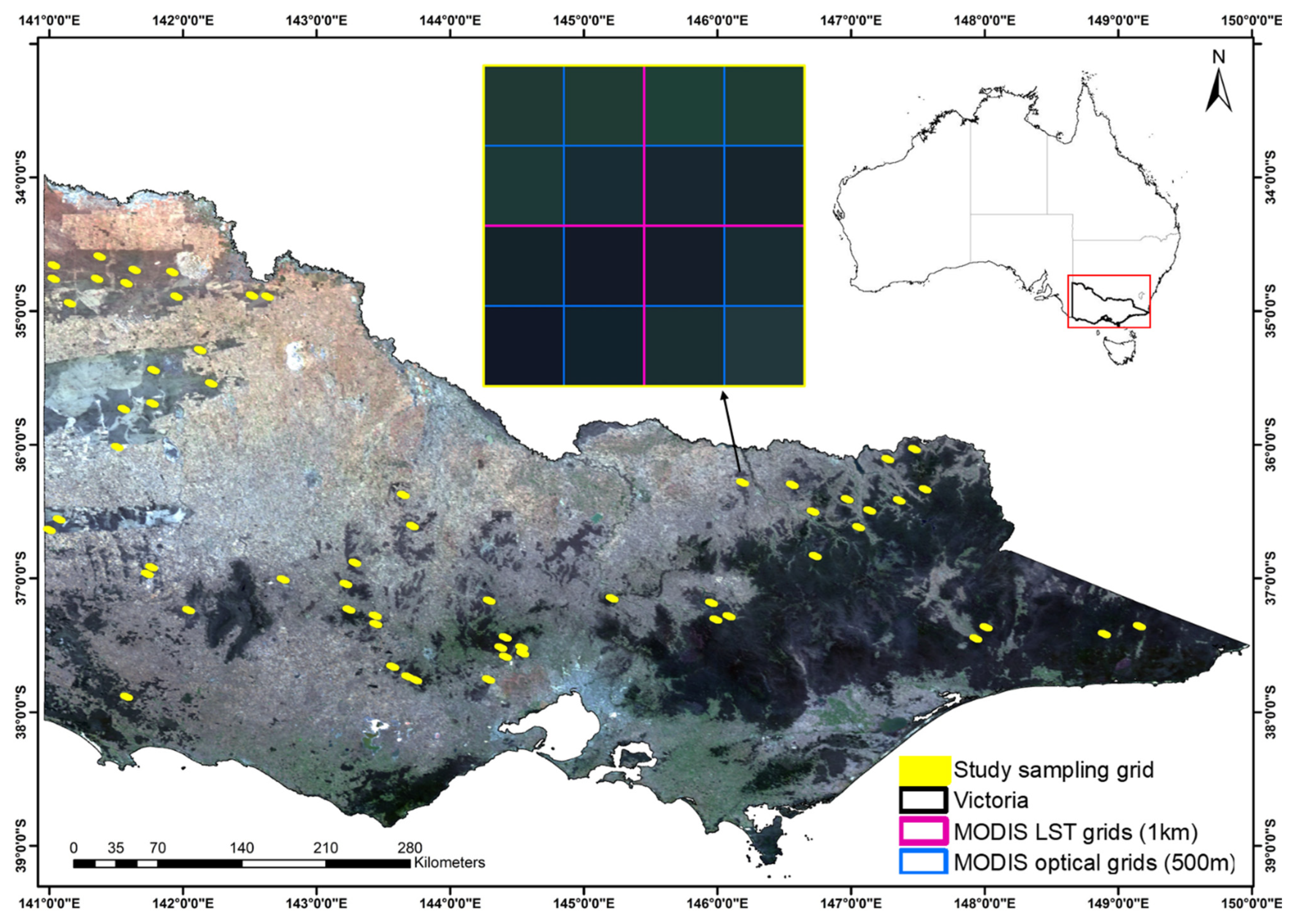
2.1. Study Area

The state of Victoria lies in the Southeastern part of Australia and has a variable climate from extremely drier western regions to wet eastern regions. The annual rainfall and temperatures range from 400 mm, 20 °C in western parts, to >1500 mm, 5 °C in eastern parts of the state [53]. The Koppen-Geiger climate type in Victoria is mainly classified as temperate and arid. The eastern and coastal regions represent a temperate climate, while the North-Western parts represent an arid climate [54]. From November to March, the temperature remains high, while from May to September, temperatures are low, and the rainfall during this period accounts for 80% of the rainfall during the whole year.

The study area encompasses a mix of eucalypt forest types, from wet montane forests in the east to sparse dry woodlands in northwest Victoria. The Ecological Vegetation Classes (EVC) is widely used as a landscape-scale classification scheme for Victoria’s vegetation types, classifying vegetation into 20 simplified native vegetation groups and 35 sub-groups [55]. These vegetation groups span a wide range of forest structural formations from low woodland to open forest and tall closed forest [56]. For the selection of the study forest patches, hereafter study sampling windows, the whole of the forest region of Victoria was sampled into spatial windows measuring (2 km × 2 km). The study sampling windows can accommodate 16 (4 × 4) pixels of MODIS–optical and 4 (2 × 2) pixels of MODIS–LST, as shown in Figure 2. The reason for selecting a study sampling window size of (2 km × 2 km) is three-fold: (1) To remove the artifacts caused by the spatial discrepancy between MODIS–optical (available at 500 m) and MODIS–LST (available at 1000 m); (2) To make spatial resolution comparable, as the modeled soil moisture data from AWRA-L, along with other meteorological data used in this study such as air temperature and vapor pressure deficit are available at 5 km spatial resolution; (3) The FLUXNET spatial location was mostly falling in the corners of the MODIS–LST/MODIS–optical pixels, so the averaging of the neighboring pixels were required.

A series of spatial analyses were executed over these study sampling windows to remove sampling windows that may have confounding data, based on the following criteria: (1) fire history (not burnt after 1990), (2) logging history (not logged after 1990), (3) continuity of forest patch (all pixels inside the sampling window should fully overlap the forest area), (4) distance from the coast (more than 30 km from the coast to avoid the continuous humid climate and probably unlimited moisture accessibility), and (5) proximity from rain gauge stations (ten or more Australian Bureau of Meteorology (BoM) rain gauge station in a radius of 30 km). As shown in Figure 2, finally, sixty study sampling windows were found suitable for historical time series analysis at the ecological level, covering large variations in aridity and vegetation densities from different species of Eucalypt.

2.2. Datasets

2.2.1. MODIS Multispectral and Thermal Infrared Dataset

MODIS, MCD43A4 version 6 Nadir Bidirectional Reflectance Distribution Function (BRDF)–Adjusted Reflectance (NBAR) dataset from the years 2002 to 2018 were used in the study [57]. This multispectral dataset is produced daily using a 16-day retrieval period available at a 500 m spatial resolution which combines data from Terra and Aqua. The LST data were extracted from MODIS dataset MYD11A1.006 [58], which provides daily Land Surface Temperature and Emissivity with 1000 m spatial resolution. The temperature values are derived from the MOD11_L2 swath product. It provides both daytime (passes around 1:30 pm local time) and nighttime (passes around 1:30 am in Australia) values accompanied by a quality layer for each. This study used daytime LST values.

The datasets are publicly available and can be downloaded through NASA Land Processes Distributed Active Archive Center (LP DAAC, see https://lpdaac.usgs.gov, accessed on 29 August 2021). The data were downloaded in bulk from NASA’s FTP server (LP DAAC FTP server, see https://e4ftl01.cr.usgs.gov/, accessed on 29 August 2021).

2.2.2. Meteorological and Model Soil Moisture Data

The modeled daily soil moisture and meteorological datasets (temperature and rainfall) and Vapour Pressure Deficit (VPD) grids at a spatial resolution of 0.05° by 0.05° were obtained from the Australian Bureau of Meteorology (BoM) for a period of 17 years (2002–2018). The daily modeled root zone soil moisture (top 1 m) from the AWRA-L model was used to develop an index and perform meta ground-truthing. AWRA-L (Australian Water Resource Assessment—Landscape) is a landscape model developed by BoM and Commonwealth Scientific and Industrial Research Organisation (CSIRO). The model runs on a daily timestep and simulates the landscape water balance for Australia from 1911 to yesterday [59]. The key outputs from the model include surface runoff, soil moisture, evapotranspiration, and deep drainage [60]. The model is validated and calibrated at distributed spatial locations using ground observed data from point-scale soil moisture probe data, flux tower estimates, and ground recharge estimates. The root zone soil moisture from BoM–AWRA-L is the sum of water in upper and lower soil layers. It represents the percentage of available water content in the top 1 m of the soil profile. Each data cell is independent of its neighbors and represents different water compartments [59,61]. The AWRA-L version 6 gives improved results, particularly for soil moisture and runoff compared to its previous version 5.

The temporal study period is from 2002 to 2018, overlapping with the millennium drought period (2002–2009) in Southeastern Australia [62]. This event allows incorporating a large variation in soil moisture from dry conditions (2002–2009) to wet conditions in 2010. Since no comprehensive field soil moisture data are available from the entire Victoria, the modeled root zone soil moisture (top 1 m) from BoM (AWRA-L) hereafter AWRA-L soil moisture were used to construct and evaluate the proposed index. AWRA-L is calibrated to observe river streamflow and evapotranspiration, and the performance of the model is assessed against gauged streamflow, in situ soil moisture, ground water recharge data, and flux-tower-based evapotranspiration [63,64]. The key evaluation metrics for AWRA-L includes, for streamflow, daily Nash–Sutcliffe efficiency (NSE): 0.49, monthly NSE: 0.67, monthly relative bias: −0.01 [65]; for soil moisture, daily correlation: 0.76, monthly correlation: 0.74 [66]; and for actual evapotranspiration, daily correlation: 0.67, monthly correlation: 0.85 [67].

2.2.3. In Situ Soil Moisture Data

The study also used measured soil moisture data for the top 85 cm of soil from four OzFlux sites located at Wombat, Wallaby, and Whroo in Victoria, and Tumbarumba in New South Wales, Australia, to validate the proposed index [67,68]. The Level 3 datasets were downloaded from the OzFlux portal (OzFlux, see http://data.ozflux.org.au/portal/, accessed on 29 August 2021).

The University of Melbourne maintains the Wombat monitoring site, which has been operational since late January 2010. The site is in a cool temperate dry sclerophyllous eucalypt forest in Central Victoria. The annual rainfall is approximately 871 mm (142-year long term average), and the temperature ranges (1–30 °C) with a mean annual air temperature (2001–2012) of 12.1 °C [69]. Wallaby flux station is located in Kinglake National Park, approximately 85 km north of Melbourne. The site’s elevation is 720 m, and the site is dominated by Mountain ash (Eucalyptus regnans). In 2009, the site was damaged by a bushfire and was re-established again in 2010. The climate is cool and temperate with an annual rainfall ranging 1100–2000 mm, and the data are available from 2005 onwards [70]. The Whroo site is located approximately 160 km north of Melbourne at the lowest elevation among all the sites, with 165 m. The mean annual precipitation as recorded by the Bureau of Meteorology at the site is 558 mm. The site is classified as the box woodland, and the data are available from 2011 to the present [71]. The Tumbarumba flux station is situated in the Bago state forest site in southeastern New South Wales. CSIRO Land and water maintain this site, and the data are available from 2001 to the present. The forest is wet sclerophyll with a mean annual rainfall of 1159 mm [67,72].

3. Methodology

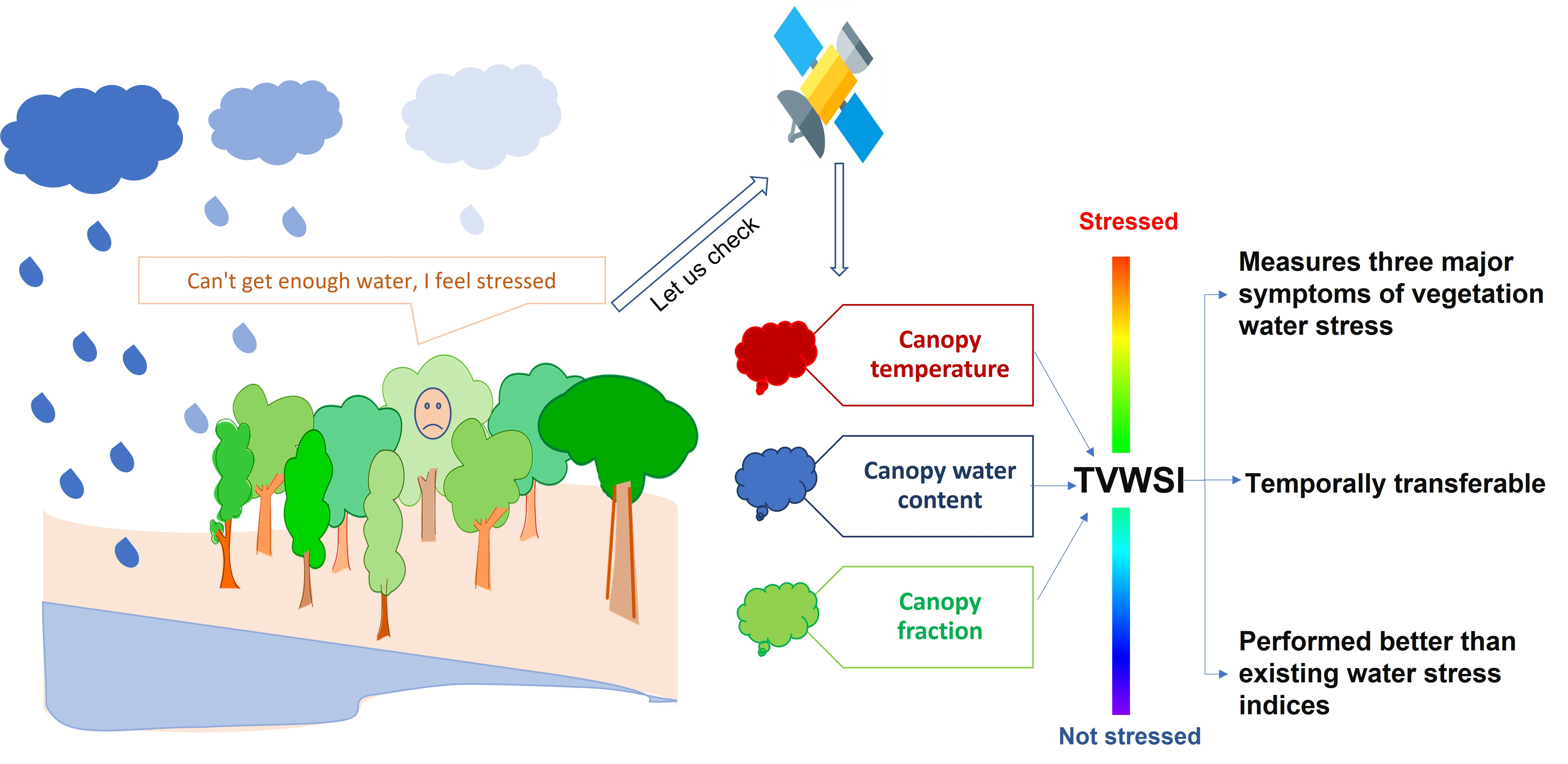
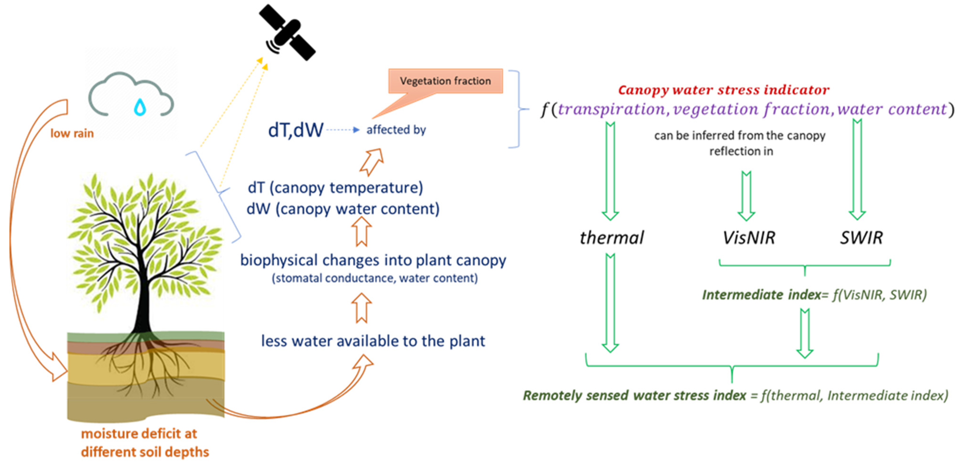
3.1. Conceptual Model: The Connection between Canopy Temperature, Canopy Water Content, and Canopy Fraction during Soil Moisture Deficits

LST can be used to characterize the increase in canopy temperatures following stomatal closure in response to water supply limitations. The magnitude of change in the canopy temperature captured by satellite sensors is also dependent on the fractional ground cover (which recognizes the proportion of evaporation and transpiration fluxes, photosynthetic activities, and canopy resistance). A key assumption is that canopy water content and canopy temperature are inversely related.

Our proposed index is presumably tested for Eucalypts water stress reactions due to limited access to soil moisture in their root zones. We assume that a decline in root-zone soil moisture will alter the stomata functioning to save water loss, accompanied by a decrease in canopy water content; further, a persistent reduction in soil moisture can alter the canopy fraction. Thus, the proposed index is designed to measure these three physiological responses from the plant under soil moisture deficit conditions in the root zone. Please note that the primary source of stress is from the root-zone soil moisture.

The proposed index (TVWSI) is a function of canopy reflection from thermal (to infer transpiration status), Visible Near Infrared (to infer vegetation fraction/photosynthetic activity), and Short-Wave Infrared (to infer vegetation water content) regions of the EM spectrum. Figure 3 shows the conceptual diagram of the roles of VisNIR, thermal, and SWIR in identifying water stress in the vegetation.

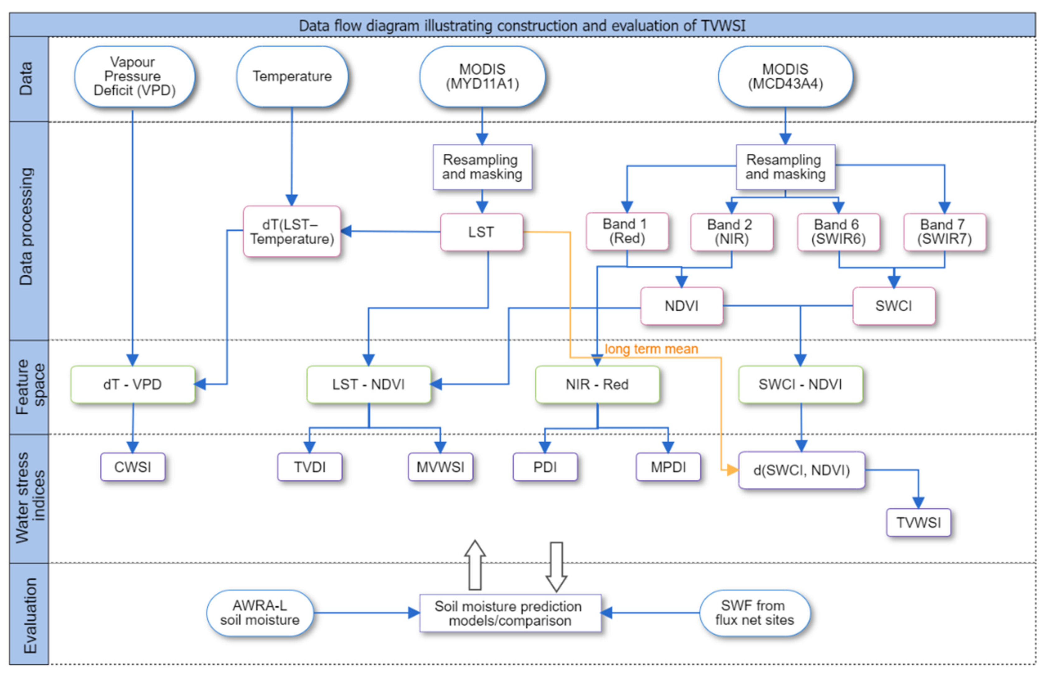
3.2. Temperature Vegetation Water Stress Index (TVWSI)

The modeling of TVWSI is described under two sections: Section 3.2.1 describes the basis for selecting the SWIR band index Surface Water Content Index (SWCI) and conceptualizing a new optical spectral space constructed using SWCI–NDVI. In addition, SWCI–NDVI was parameterized, and a new intermediate index, d(SWCI, NDVI), was devised using NDVI and SWCI spectral space. Further to this, Section 3.2.2 describes the modeling of the TVWSI, using the modeling concept of MVWSI, by replacing NDVI with d(SWCI, NDVI).

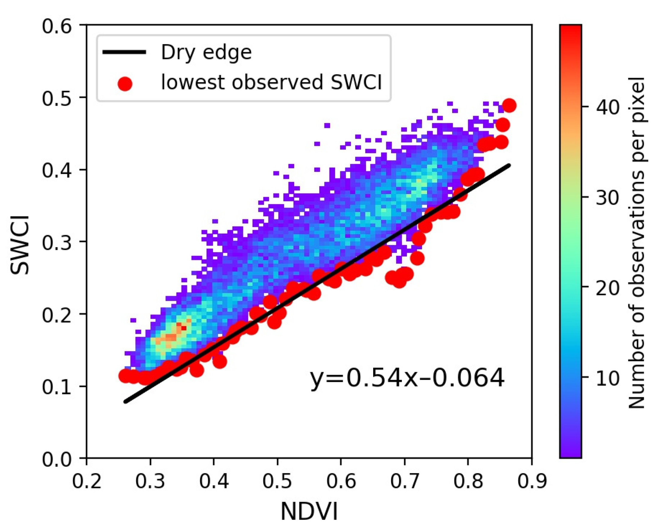
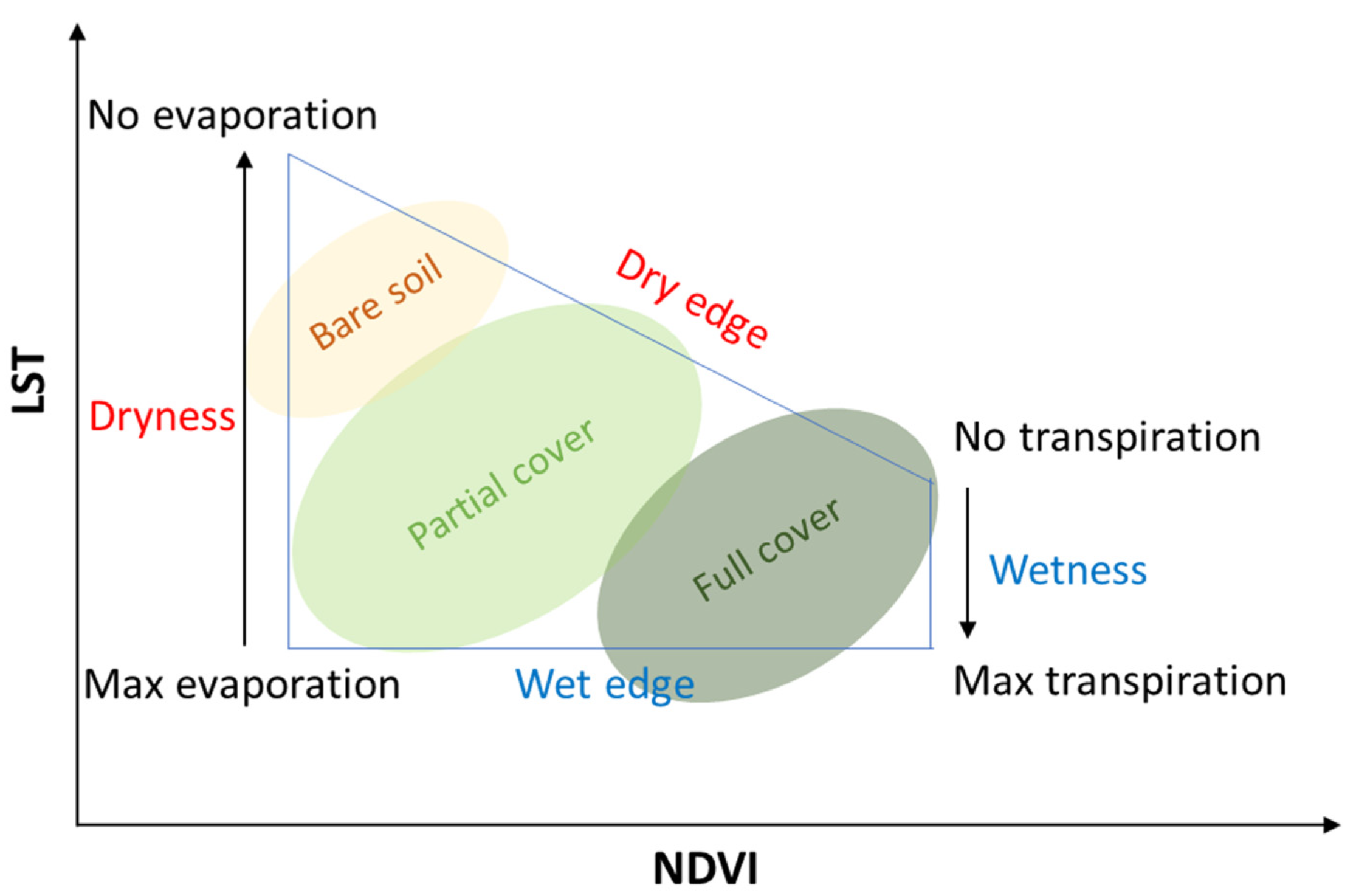
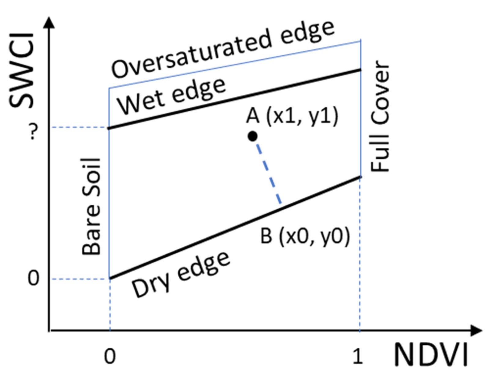
3.2.1. SWCI–NDVI Spectral Space and Derivation of d(SWCI, NDVI)

In developing our index, atmospherically stable multi-SWIR channel indices were given preference over a single SWIR channel to deal with errors from atmospheric water vapor [73,74]. SWCI was selected as the candidate SWIR index to augment NDVI. SWCI was developed to estimate vegetation canopy water content dynamics regulated by changes in soil moisture content, and it was used by numerous studies to estimate surface soil moisture [75,76]. The metric is the normalized ratio between SWIR (B₆) and SWIR (B₇) of MODIS, where B_n is MODIS band n and R_m represents the reflectance of waveband with a wavelength m in µm.

$$\mathrm{SWCI}=\frac{R_{1.65}-R_{1.9}}{R_{1.65}+R_{1.9}} ~\frac{B_6-B_7}{B_6+B_7}$$

(1)

SWCI uses bands near the absorption valley and peak of the water spectra; therefore, the difference of these bands should increase with vegetation water content. As both bands have the same atmospheric scattering and radiation values, taking the normalized ratio reduces the atmosphere’s effect on their individual bands [77,78].

The Normalized Difference Vegetation Index (NDVI) uses Red and NIR channels from the EM spectrum [79]. It is widely used to estimate vegetation growth parameters such as LAI, greenness, photosynthetic activeness, vigor, and phenology. MODIS Band ($B_1$) and Band ($B_2)$ from the MODIS were used to calculate NDVI, R represents the radiance in reflectance units.

$$\mathrm{NDVI}=\frac{R_{0.86}-R_{0.645}}{R_{0.86}+R_{0.645}} ~\frac{B_2-B_1}{B_2+B_1}$$

(2)

We assume a linear relationship between root zone soil moisture and vegetation canopy water content. This assumption conforms to previous studies that have used remotely sensed vegetation indices to quantify plant vigor and relate it to root zone soil moisture [80,81,82,83,84,85]. As for LST–NDVI, a feature space of SWCI–NDVI can be constructed, as shown in Figure 4. This figure is adopted from Sadeghi et al. [86], who used a similar feature space constructed using shortwave infrared transformed reflectance (STR) –NDVI to estimate root-zone soil moisture. It is to be noted that the reflection in the SWIR region is sensitive to canopy water content and the pooled water on the surface. The meaningful relationship between root-zone soil moisture and SWCI is valid for partially or fully saturated soil but not beyond this state (i.e., when water accumulates on the soil surface). Although SWCI will continue to increase with standing water, that does not mean that soil moisture is increasing, as it is bound to a certain maximum limit (saturation). This issue was pointed out in defining the wet edge in optical spectral space; hence, there must be some assumptions for the upper SWCI values corresponding to the maximum limit of soil moisture, shown by (?) in Figure 4 (oversaturated edge). Therefore, we only used the dry edge to remove this ambiguity while defining the new index.

Suppose a hypothetical dry line can be drawn in the spectral space of SWCI–NDVI, as shown in Figure 4. In that case, the perpendicular distance of observations to this line can represent soil moisture content, i.e., the distance of observation to this line will increase with soil water content. The dryline can be estimated by fitting a linear regression line on the lowest SWCI from NDVI bins across the x-axis. The number of bins in the NDVI range can be estimated using the method proposed by Sturges [87]. The method states that for a series of range R with N items, the optimal class interval (bins) may be estimated from the formula:

$$class interval \left(bins\right)=\frac{R}{1+3.322 {\log }_{10}N}$$

(3)

Let us suppose the equation of the dry edge is given by

$$y=mx+c$$

(4)

where m is slope and c is the intercept of the line.

Then a perpendicular line to dry edge, passing through A ($x_i, y_i$) can be given as

$$\left(y-y_i\right)=-\frac{1}{m}\left(x-x_i\right)$$

(5)

the perpendicular distance AB from a point A ($x_i, y_i$) to dry edge can be derived as

$$\mathrm{AB}=\frac{y_i-m{x}_i-c}{\sqrt{m^2+1}}$$

(6)

Therefore, the perpendicular distance corresponding to the ith observation of NDVI and SWCI, denoted as $\mathrm{d}\left({\mathrm{SWCI}}_i,{ \mathrm{NDVI}}_i\right)$, was calculated as

$$\mathrm{d}\left({\mathrm{SWCI}}_i, {\mathrm{NDVI}}_i\right)=\frac{{\mathrm{SWCI}}_i-m{\mathrm{NDVI}}_i-c}{\sqrt{m^2+1}}$$

(7)

This perpendicular distance may account for the effect of vegetation fraction (due to NDVI) and canopy water content (due to SWCI) concurrently and can be linked more efficiently than NDVI and SWCI to the ground soil moisture conditions.

3.2.2. Derivation of TVWSI

TVWSI is based on the theoretical principle of the modified version of the simple ratio index VWSI (NDVI/LST) [21,35,36]. It is the most straightforward derivation of the slope from the LST–NDVI feature space. Numerous studies have found that LST–NDVI slope dynamics are sensitive to plant-available soil moisture and plant water stress [17,19,21,25,88], while other studies have found a significant relation between VWSI and vegetation water supply, which can directly link to soil moisture conditions, transpiration regimes, and vegetation water stress [36]. A study by McVicar and Bierwirth [41] over Papua New Guinea suggested that the ratio of NDVI and LST is a direct measure of the drought.

The major limitation in using LST on spatio-temporal data is its dependency on the region-specific properties such as canopy structure and ambient atmospheric conditions such as air temperature and wind speed. However, a study by Wu and Lu [37] found that the relative LST, i.e., the real-time LST divided by long term mean of LST corresponding to that time and region, can solve this limitation. Consequently, we employed relative LST instead of LST to construct a spatially transferrable vegetation water stress index.

The standardized LST or relative LST denoted by RLST is the ratio of LST with its long-term mean ($\overline{\mathrm{LST}}$). This mathematical conversion of LST makes its application feasible in time and space.

$$RLST=\frac{\mathrm{LST}}{\overline{\mathrm{LST}}}$$

(8)

TVWSI is devised by employing d(SWCI, NDVI) in place of NDVI in the model of MVWSI and is given by:

$$\mathrm{TVWSI}=\frac{\mathrm{d}\left(\mathrm{SWCI}, \mathrm{NDVI}\right)}{RLST}$$

(9)

Retrieving changes in soil moisture using TVWSI will depend on the dynamics of d(SWCI, NDVI) and LST during varying soil moisture conditions. Under normal soil moisture conditions, both d(SWCI, NDVI) and LST are expected to vary in some reasonable range; d(SWCI, NDVI) should have relatively higher values, and LST should have relatively smaller values. Overall, TVWSI will have a relatively high value for high soil moisture conditions. In contrast, under water-limited conditions, LST increases due to less evaporative cooling, and correspondingly, d(SWCI, NDVI) decreases due to a reduction in water content and vegetation growth, resulting in a decrease in the slope of SWCI–NDVI spectral space.

3.3. Evaluation of TVWSI

A comparative analysis was performed between TVWSI and existing vegetation water stress indices, based on their skills to predict AWRA-L soil moisture from sixty sampling study windows and observed Soil Water Fraction (SWF) from four FLUXNET sites. First-, second-, and third-order polynomial models were fitted between the indices and AWRA-L soil moisture/SWF. Then, Root Mean Square Error (RMSE) (predicted AWRA-L soil moisture/SWF vs. actual AWRA-L soil moisture/SWF), Mean Absolute Percentage Error (MAPE) (predicted AWRA-L soil moisture/SWF vs. actual AWRA-L soil moisture/SWF), and R² (predicted AWRA-L soil moisture/SWF vs. actual AWRA-L soil moisture/SWF) were used to compare the skills of the water stress metrics in estimating soil moisture.

Table 1. Indices evaluated against TVWSI. For Perpendicular Dryness Index (PDI) and modified Perpendicular Dryness Index (MPDI), $R_{ Red}, R_{NIR}$ represents the reflectance in red and NIR region, $R_{v, Red}, R_{v,NIR}$ represents vegetation reflectance in Red and NIR region, M represents the slope of the soil line, $f_v$ represents vegetation fraction. For Modified Vegetation Water Supply Index (MVWSI), RLST represents the ratio of LST with its long-term mean. For Temperature Vegetation Dryness Index (TVDI), $T_s$ and $T_{s_{min}}$ represents surface temperature and minimum temperature along the wet edge, a and b are parameters defining the dry edge. For the Crop Water Stress Index (CWSI), $\left(T_c-T_a\right)$ represents the temperature difference between canopy and air, ${(T_c-T_a)}_l$ represents the lower non-water-stressed boundary, and ${(T_c-T_a)}_u$ represents the upper reference non-transpiring condition boundary.

Indices	References
$\mathrm{PDI}=\frac{1}{\sqrt{M^{2 }+1}}\left(R_{Red}+M{R}_{NIR}\right)$	[45]
$\mathrm{MPDI}=\frac{(R_{Red}+M{R}_{NIR}-f_v\left(R_{v,Red}+M{R}_{v,NIR}\right)}{\left(1-f_v\right)\sqrt{M^{2 }+1}}$	[46]
$\mathrm{MVWSI}=\frac{NDVI}{RLST}$	[37]
$\mathrm{TVDI}=\frac{T_s-T_{s_{min}}}{a+bNDVI-T_{s_{min}}}$	[18]
$\mathrm{CWSI}=\frac{\left(T_c-T_a\right)-{(T_c-T_a)}_l}{{(T_c-T_a)}_u-{(T_c-T_a)}_l}$	[89]

shows the existing water stress indices against which TVWSI was evaluated.

The dataflow diagram describing the construction and evaluation of TVWSI is shown in Figure 5.

4. Results

The proposed indices were evaluated using 17-year (2002–2018) weekly AWRA-L soil moisture from sixty study sampling windows and Soil Water Fraction (SWF) from the four FLUXNET stations. The daily data were converted into a weekly temporal resolution to deal with outliers or errors in the daily datasets. The weekly maximum NDVI, SWCI and mean LST, AWRA-L soil moisture, and SWF were considered for the analysis. The analysis was confined to the summer season (December to February) as these are the months are when vegetation may be exposed to soil moisture deficits and more likely to experience water stress. We assume that root zone soil moisture (moisture in the top 1 m of soil) is the primary driver of vegetation water stress. Separate regression analyses were performed between the proposed and existing water stress indices (that we consider are the remotely sensed indicator of vegetation water stress) and AWRA-L soil moisture. The comparison of proposed indices was made with the existing vegetation water stress indices, presented, and discussed in the following sections.

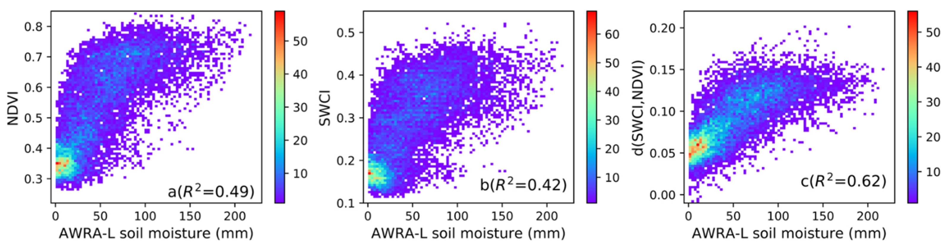
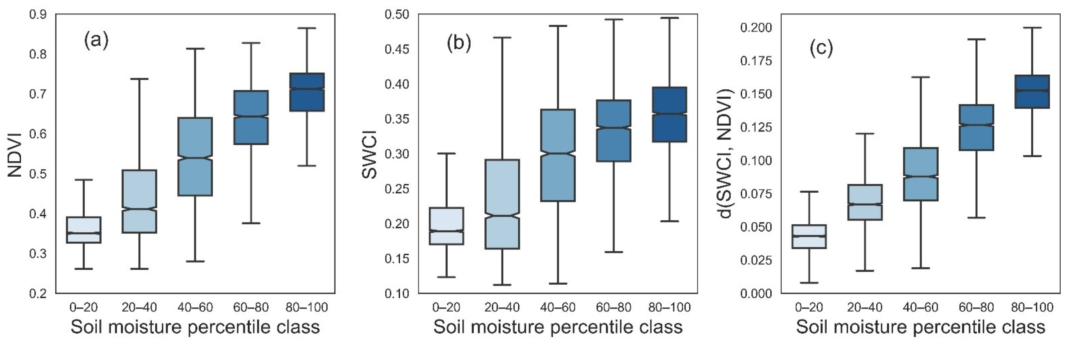
4.1. Estimation of d(SWCI, NDVI) from SWCI–NDVI Spectral Space and Analysis of Correlation with AWRA-L Soil Moisture

To calculate the dry edge in SWCI–NDVI spectral space, the NDVI were classified into different bins across the x-axis. The number of bins was calculated using the formula proposed by Sturges [87]. Then, in each bin of the NDVI, the lowest SWCI was identified, and a linear regression line fitted to these points (Figure 6). Finally, the distance d(SWCI, NDVI) of each observation to this lowest slope line was calculated by the method described in Section 3.2.

Figure 7 shows the density scatter plots of NDVI, SWCI, and d(SWCI, NDVI) vs. AWRA-L soil moisture with their corresponding R² value. The shape of the plot and R² score suggest that NDVI, SWCI, and d(SWCI, NDVI) have a positive correlation with AWRA-L soil moisture, and d(SWCI, NDVI) has significantly improved the correlation and the linearity of the relationship compared with NDVI and SWCI. In addition, Figure 7c confirms our assumption that the distance of an observation relative to the lowest slope line in NDVI–SWCI spectral space increases with soil moisture.

In order to analyze the improvements d(SWCI, NDVI) bought over NDVI and SWCI, we classified the data from sixty study sampling windows into five classes representing 0–20, 20–40, 40–60, 60–80, and 80–100 soil moisture percentile. Then, the ranges of each of the indices NDVI, SWCI, and d(SWCI, NDVI) was estimated for each of these soil moisture percentile classes, shown by the boxplots in Figure 8. These boxplots suggest d(SWCI, NDVI) improved the skills of NDVI and SWCI in separating different ranges of soil moisture, especially at the end members of soil moisture, i.e., at lower (0–20) and upper (60–100) ranges (Figure 8c). These results suggest the distance metric may have higher skill for retrieving soil moisture dynamics in drier and wetter zones where other vegetation indices such as NDVI and SWCI generally saturates or is contaminated by background noise [90,91,92].

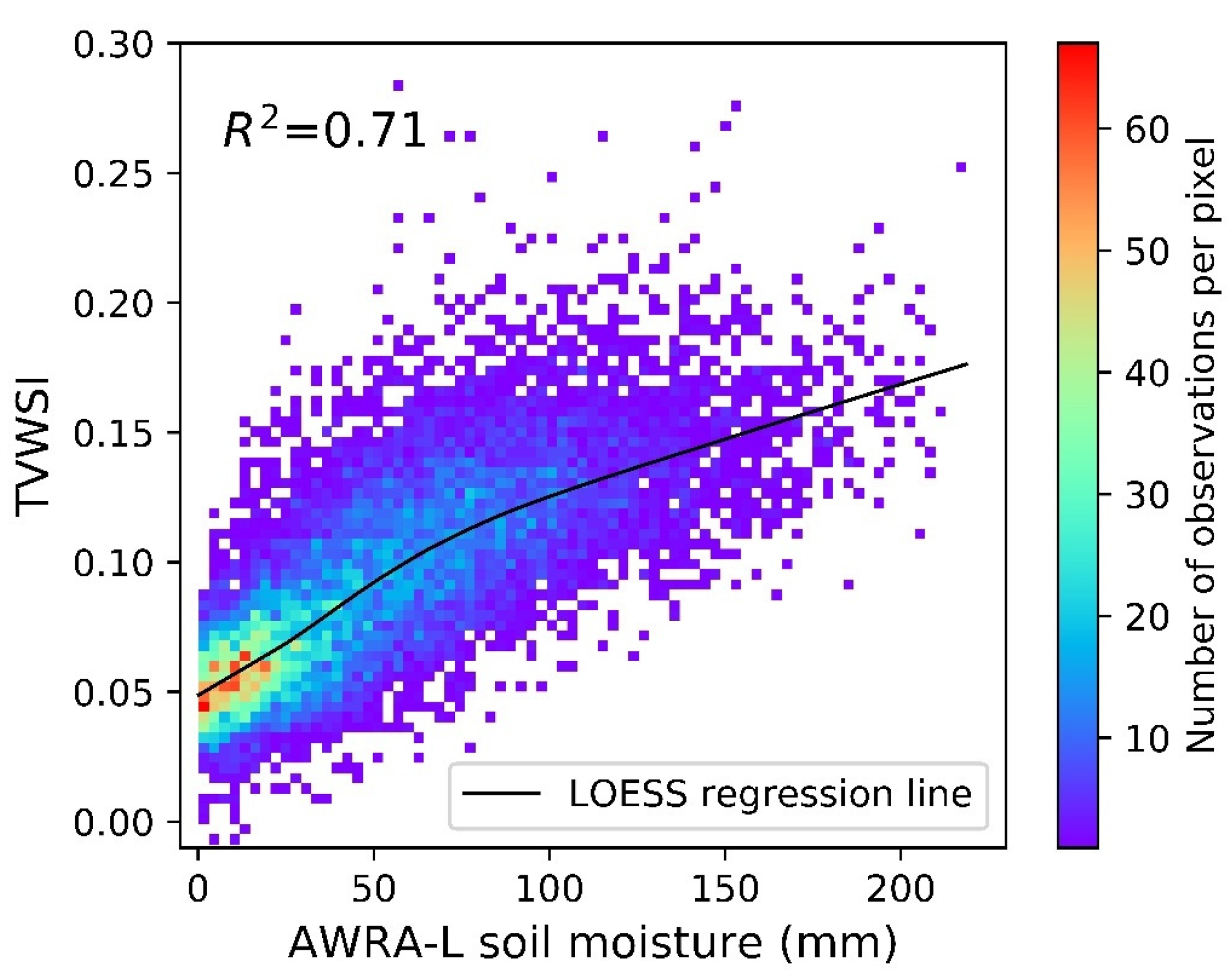
4.2. Estimation of TVWSI and Analysis of Correlation with AWRA-L Soil Moisture

The construction of TVWSI is based on the LST–NDVI slope relationship with soil moisture. The simpler model of the LST–NDVI slope is their ratio (NDVI/LST). The principle behind the working of this ratio is the energy partitioning between vegetative and non-vegetative surfaces, which NDVI can identify for LST. In order to overcome the limitation of LST dependency on ambient atmospheric conditions, we employed the method proposed by Wu and Lu [37], who used standardized LST instead of LST. Further, we replaced NDVI with d (SWCI, NDVI) in the model of MVWSI to construct TVWSI.

TVWSI showed the highest correlation with AWRA-L soil moisture than its input parameters: NDVI, SWCI, d(SWCI, NDVI), and LST. The coefficient of determination (R²) of AWRA-L soil moisture vs. TVWSI, NDVI, SWCI, d(SWCI, NDVI), and LST are 0.71, 0.49, 0.42, 0.62, and 0.51, respectively. Figure 9 shows the density scatter plot of TVWSI vs. AWRA-L soil moisture.

The locally estimated scatterplot smoothing (LOESS) shown in Figure 9 suggests that TVWSI has the sensitivity to estimate both low and high soil moisture events, with a slight tendency to underestimate soil moisture after around 75 mm. In comparison, the interannual variability in TVWSI also suggests its capability to identify these extremes, i.e., lowest and highest rainfall years. For example, the summer of 2006 was the driest year during the millennium drought (1997–2009) in SE Australia; TVWSI is relatively low in this time and has identified this driest year efficiently (Figure S1). In contrast, the millennium drought ended with massive flood events in 2010; TVWSI has also identified this wet event efficiently, which is reflected by the highest value of TVWSI in 2010 (Figure S1).

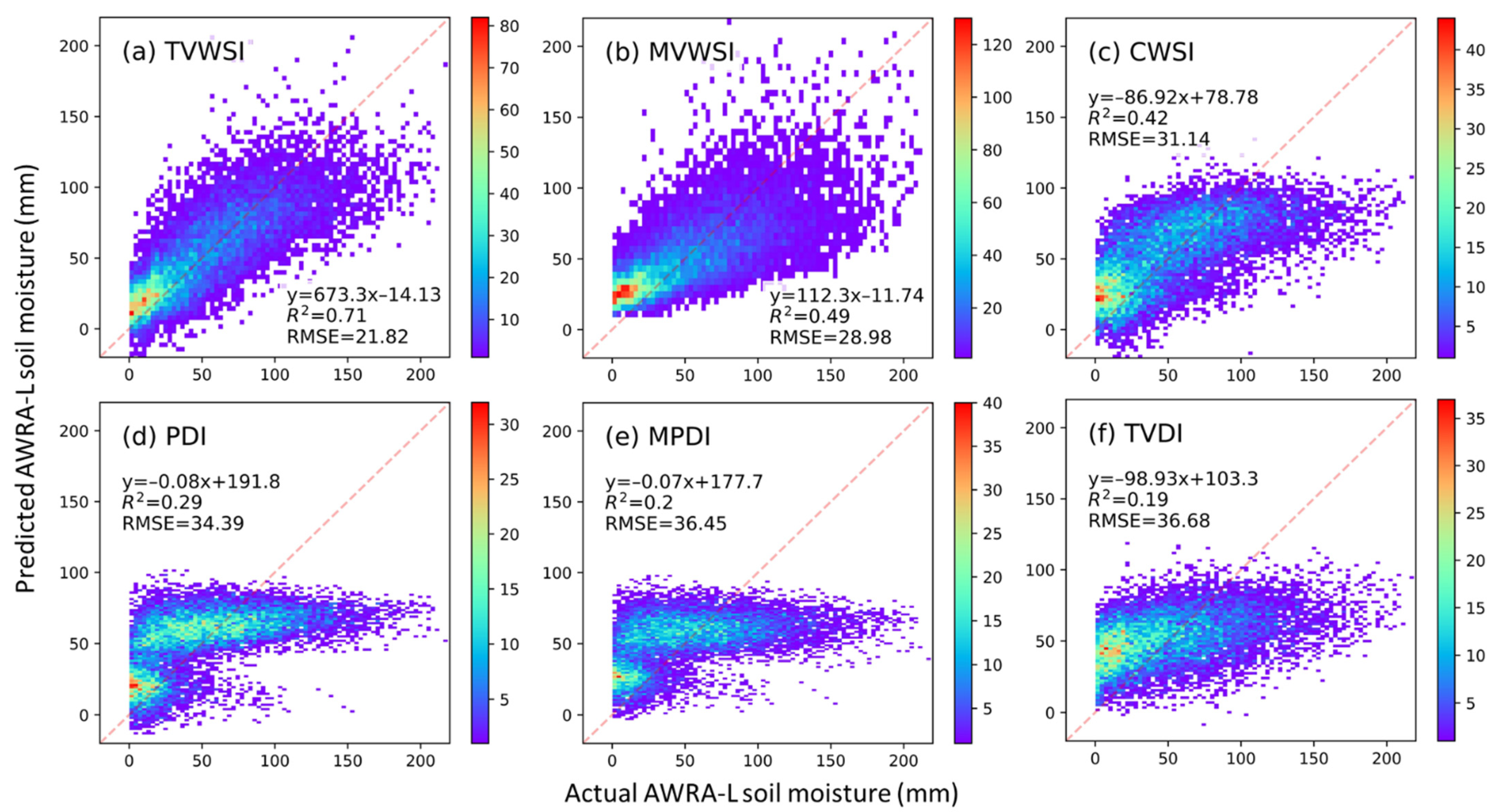
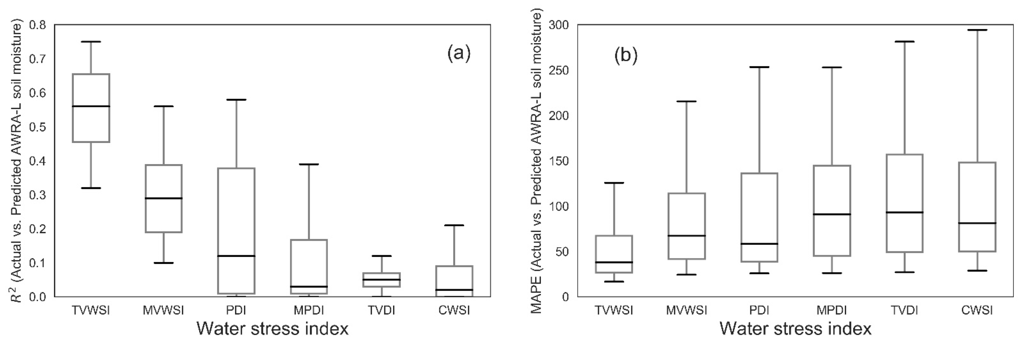
4.3. Evaluation of TVWSI in Predicting AWRA-L Soil Moisture, and Comparison with Existing Water Stress Metrics

This section presents a comparative analysis between TVWSI and other existing water stress indices in predicting AWRA-L soil moisture. The first-, second-, and third-order polynomial models were developed for TVWSI, PDI, MPDI, MVWSI, TVDI, and CWSI, to predict AWRA-L soil moisture. R² and RMSE between actual vs. predicted AWRA-L soil moisture were used to compare the performances of these indices. The seventeen-year weekly data from sixty study sampling windows were randomly divided into 70% and 30% sample sizes. The sample size comprising 70% of data was used to train the model, while the remaining 30% was used to predict AWRA-L soil moisture. This procedure was repeated 10,000 times on the different sets of randomly selected training and testing data samples. The R² and RMSE reported are the averages of the outcomes of these iterations. Boxplots show the range of R² and RMSE obtained by running 10,000 iterations in Figure S2. Figure 10 shows the density scatter plot (Actual AWRA-L soil moisture vs. Predicted AWRA-L soil moisture) with the model equation, R² and RMSE, corresponding to the first-order polynomial model for each index. In comparison, the model performance measures (R² and RMSE) from the second- and third-order polynomial models are shown in

Table 2. R² (index vs. AWRA-L soil moisture) and RMSE (Actual vs. Predicted AWRA-L soil moisture) corresponding to the first-, second-, and third-order polynomial model fitted to AWRA-L soil moisture vs. TVWSI, MVWSI, CWSI, PDI, MPDI, and TVDI.

VI’s	Actual vs. Predicted AWRA-L Soil Moisture (R2)			RMSE (mm)
	1st-Order Polynomial Model	2nd-Order Polynomial Model	3rd-Order Polynomial Model	1st-Order Polynomial Model	2nd-Order Polynomial Model	3rd-Order Polynomial Model
Proposed vegetation water stress index
TVWSI	0.71	0.71	0.72	21.82	21.8	21.38
Existing vegetation water stress indices
MVWSI	0.49	0.54	0.55	28.98	27.51	27.44
CWSI	0.42	0.42	0.43	31.14	30.89	30.71
PDI	0.29	0.29	0.31	34.39	34.27	33.70
MPDI	0.20	0.20	0.23	36.45	36.36	35.80
TVDI	0.19	0.19	0.20	36.68	36.53	36.49

.

The soil line in the NIR–Red and the dry edge in the LST–NDVI feature space were estimated to calculate PDI, MPDI, and TVDI from NIR–Red and LST–NDVI feature spaces.First, the values of Red-reflectance were divided into the class intervals to generate a soil line in the NIR–Red spectral space. The number of intervals was defined by the method proposed in Sturges [87]. Similarly, NDVI values were divided into classes to generate the dry edge in the LST–NDVI feature space; then, PDI and MPDI were extracted from NIR–Red and TVDI were computed using the LST–NDVI feature space.

Figure 10 and Table 2 clearly show that TVWSI (R² = 0.71, RMSE = 21.82) has the highest linear correlation with AWRA-L soil moisture. TVDI performed worst in predicting soil moisture, followed by MPDI and PDI. These three indices lost sensitivity at high soil moisture, which can be observed from the flattening of scatter plots at the higher soil moisture, as shown in Figure 10d–f. Apart from MVWSI, none of the indices has shown any noticeable enhancement in predicting AWRA-L soil moisture with higher-order polynomial models.

The prediction abilities of indices to AWRA-L soil moisture were also estimated across each of the sixty individual study sampling windows. The R² and mean absolute percentage error (MAPE) ranges corresponding to each water stress index are shown by the boxplot in Figure 11. Notably, for PDI, MPDI, TVDI, MVWSI, and CWSI, many sampling windows showed weak or no correlation with R² as low as 0 for PDI, MPDI, TVDI, CWSI, and 0.1 for MVWSI. This weakening of relationship at individual study sampling window suggests that large observed data points are required to parameterize these indices. On the other hand, the MAPE is as high as greater than 300% for PDI, MPDI, and CWSI and greater than 250% for MVWSI and TVDI. The performance of TVWSI was relatively better across the sampling study windows, with the lowest R² of 0.31 and the highest MAPE of 145%, which is significantly less than other indices.

4.4. Evaluation of TVWSI in Predicting Soil Water Fraction (SWF) from Flux Tower Data, and Comparison with Existing Water Stress Metrics

The proposed water stress index was evaluated against the existing indices in predicting soil water fraction from four contrasting FLUXNET sites across Victoria and New South Wales. The first-, second-, and third-order polynomial functions were fitted using soil water fraction as the dependent variable and the indices as an independent variable. The scatter plots in Figure 12 show the observed vs. predicted soil water fraction from four FLUXNET sites using the first-order polynomial model, along with R², RMSE, and model equation. R² and RMSE are the averages of the outcomes obtained after 10,000 iterations on the randomly selected training and testing datasets. CWSI was not calculated over FLUXNET stations due to the unavailability of vapor pressure deficit.

TVWSI showed improved prediction skills for SWF than other indices at Wombat, Wallaby, and Tumbarumba FLUXNET sites and slightly better at Whroo (

Table 3. R² (index vs. soil water fraction) and RMSE (observed vs. predicted Soil Water Fraction) at each of the four FLUXNET sites Whroo, Wallaby, Wombat, and Tumbarumba, corresponding to the 1st-order polynomial function fitted to Soil Water Fraction vs. TVWSI, MVWSI, TVDI, PDI, and MPDI.

Vegetation Water Stress Index	Whroo		Wallaby		Wombat		Tumbarumba
	R2	RMSE	R2	RMSE	R2	RMSE	R2	RMSE
TVWSI	0.25	0.029	0.43	0.024	0.51	0.032	0.44	0.040
MVWSI	0.21	0.035	0.20	0.029	0.33	0.038	0.23	0.047
TVDI	0.20	0.035	0.29	0.027	0.24	0.040	0.17	0.048
PDI	0.08	0.038	0.10	0.030	0.32	0.038	0.00	0.053
MPDI	0.07	0.038	0.10	0.030	0.27	0.039	0.00	0.053

). Tumbarumba and Wallaby sites are the wettest sites where the forest type is classified as a temperate evergreen wet sclerophyll forest [70,72]. These energy-limited systems with continuous access to soil moisture show minimal deviations in the greenness. This is evident from the NDVI range over these forests, which ranges between 0.65 and 0.8. The low performance of the indices over Tumbarumba might have been due to the saturation of red reflectance and thus NDVI at high biomass [93,94] or its considerable lag with soil moisture [90,95]. The improved performance of TVWSI in predicting SWF could be due to the presence of SWCI in its model, which can perceive changes in canopy water content even from higher vigor canopy.

The poor performance of PDI and MPDI at Whroo could be due to the absence of LST in its model. In contrast, the relatively better performance of the indices that include LST in their model may be related to the high correlation of LST and surface soil moisture content in the driest regions with open-canopy forests [96,97,98]. The relationship of LST and soil moisture content generally gets decoupled and becomes more complex at the wetter sites such as Tumbarumba and Wallaby because dense closed forest canopies usually characterize the wetter sites. A considerable amount of variations in the canopy temperature come from the canopy structure and background soil viewed to the sensor [35]. Therefore, to efficiently estimate soil moisture content, there should be a clear partitioning between temperature sensed from the canopy and the background soil, which is still a significant limitation of the satellite remote sensing [99].

5. Discussion

NDVI and SWCI are the indirect indicators of soil moisture over the vegetative surface. Their functioning depends on the biophysical links between soil moisture dynamics and its feedback with the vegetation canopy. NDVI correlates with soil moisture because of high vegetation fractions in wetter regions and vice versa. In comparison, the SWCI’s association with soil moisture is based on a linear relationship between soil and vegetation water content. Situations could exist in a forest ecosystem when the vegetation fraction at two different locations is the same, but soil moisture is different. These scenarios can be well estimated by combining the indicator of vegetation fraction and vegetation water content. Replacing LST by SWCI in the LST–NDVI trapezoid has fulfilled this inability of NDVI.

The index d(SWCI, NDVI) is more sensitive than NDVI and SWCI at the lower and higher end of the soil moisture spectrum. The boxplots shown in Figure 8 demonstrates that d(SWCI, NDVI) has improved retrieval of soil moisture dynamics at the lower and higher ranges of soil moisture. This capability of retrieving soil moisture at extreme ends is a significant improvement over NDVI, which generally saturates and tends to represent a general nature of lagged canopy response to root zone soil moisture [90,91,92,95,100]. The improved correlation of soil moisture vs. d(SWCI, NDVI) at the higher and lower moisture regions could also be due to SWCI in its model, which can perceive water dynamics from the canopy and the soil [101].

TVWSI was constructed using d(SWCI, NDVI) and LST, and it is based on the theoretical principle of MVWSI, which is a simple derivation of slope from LST–NDVI and is sensitive to plant available water [21,35,37,101]. However, LST’s dependence on ambient atmospheric conditions is the major limitation of parameterizing LST–NDVI spectral space on temporal observations. That is why we have extracted the parameters using SWCI–NDVI spectral space and then combined the extracted intermediate index with the standardized LST. TVWSI has shown significant improvement in R² and linearity with AWRA-L soil moisture over d(SWCI, NDVI), as shown in Figure 7c and Figure 9. The reason could be that the recent rainfall abruptly increases soil moisture in the root zone and decreases the canopy temperature, which LST can perceive efficiently compared to the optical reflection. TVWSI has also shown sensitivity to the wettest and driest events during the millennium drought, as shown in Figure S1. This capability of TVWSI makes it a reliable indicator of root zone soil moisture, and we contend that TVWSI can be employed to estimate drought intensity.

The improved performance of TVWSI in predicting AWRA-L soil moisture and soil water fraction shows its superiority over other the existing water stress indices compared in this paper. The improvement over PDI and MPDI demonstrates that optical reflectance on its own is not a good predictor of soil moisture dynamics in the root zone. LST is a subtle measure of plant water stress, and LST’s sensitivity to transpiration cannot be realized by optical reflectance. The improvement over TVDI can be explained by the fact that LST depends on the ambient atmospheric condition. That is why the spectral space of LST–NDVI cannot be globally parameterized for the temporal observations. In comparison, the improvement of TVWSI over CWSI and MVWSI could be due to the inclusion of canopy water content, which is missing in the models of MVWSI and CWSI.

TVWSI’s performance decreased when applied to the prediction of point-scale SWF values from ground monitoring sites when compared to AWRA-L soil moisture. This may be due to the large discrepancy in their support scales. It had a superior skill in root-zone soil moisture prediction compared with the other indices. This study has considered an area of (2 km × 2 km) for the study sampling windows, which could be spatially comparable with AWRA-L (approximately 5 km × 5 km), but their spatial representation is far greater than the “point” scale ground soil moisture measurements. Furthermore, studies have shown that the soil moisture features very high spatial variability, changing even at the scale of meters for the surface soil moisture [102]. Therefore, it could be assumed that the point measurement is not representative of a 2 km × 2 km footprint. The other potential cause could be that SWF was measured at variable soil depth across the year, and also, the method to calculate SWF across different sites are different [67]. The data availability was also not continuous across the sites; for example, the availability of data was Wombat (2010–2021), Wallaby (2005–2013), Whroo (2011–2021), and Tumbarumba (2001–2021).

6. Conclusions

This study investigated the hypothesis that an improved water stress index could be constructed by representing canopy water content information to the LST–NDVI trapezoid model. Moreover, the LST–NDVI feature space cannot be used to parameterize temporal observations due to LST’s dependency on ambient atmospheric conditions. The following conclusions can be made from the study:

• The intermediate vegetation index d(SWCI, NDVI) is modeled using NDVI and SWCI to simultaneously consider the effects of vegetation growth and vegetation water content. d(SWCI, NDVI) showed an improved correlation with AWRA-L soil moisture than NDVI and SWCI. Moreover, d(SWCI, NDVI) improved retrieving soil moisture dynamics at the lower and higher ranges of soil moisture, which is a significant improvement over the saturation nature of NDVI over high-density vegetation and its inability on open canopy regions;
• Compared to PDI, MPDI, MVWSI, TVDI, and CWSI, the newly devised TVWSI improved prediction ability for the modeled AWRA-L root zone soil moisture from sixty study sampling windows and soil water fraction (SWF) from the four contrasting FLUXNET sites across Victoria and New South Wales;
• As the optical spectral space of SWCI–NDVI and standardized LST is used to model TVWSI, it can be employed to estimate soil moisture dynamics on the temporal data.

References

1. Allen, C.D.; Macalady, A.K.; Chenchouni, H.; Bachelet, D.; McDowell, N.; Vennetier, M.; Kitzberger, T.; Rigling, A.; Breshears, D.D.; Hogg, E.H.; et al. A global overview of drought and heat-induced tree mortality reveals emerging climate change risks for forests. Forest Ecol. Manag. 2010, 259, 660–684. [Google Scholar] [CrossRef] [Green Version]
2. Zhang, Y.; Peng, C.; Li, W.; Fang, X.; Zhang, T.; Zhu, Q.; Chen, H.; Zhao, P. Monitoring and estimating drought-induced impacts on forest structure, growth, function, and ecosystem services using remote-sensing data: Recent progress and future challenges. Environ. Rev. 2013, 21, 103–115. [Google Scholar] [CrossRef]
3. Yao, Y.; Liang, S.; Cao, B.; Liu, S.; Yu, G.; Jia, K.; Zhang, X.; Zhang, Y.; Chen, J.; Fisher, J.B. Satellite detection of water stress effects on terrestrial latent heat flux with MODIS shortwave infrared reflectance data. J. Geophys. Res. Atmos. 2018, 123, 11–410. [Google Scholar] [CrossRef] [Green Version]
4. Evans, B.; Stone, C.; Barber, P. Linking a decade of forest decline in the south-west of western Australia to bioclimatic change. Aust. For. 2013, 76, 164–172. [Google Scholar] [CrossRef]
5. Fensham, R.J.; Fairfax, R.J.; Butler, D.W.; Bowman, D.M.J.S. Effects of fire and drought in a tropical eucalypt savanna colonized by rain forest. J. Biogeogr. 2003, 30, 1405–1414. [Google Scholar] [CrossRef]
6. Fensham, R.J.; Fairfax, R.J. Drought-related tree death of savanna eucalypts: Species susceptibility, soil conditions and root architecture. J. Veg. Sci. 2007, 18, 71–80. [Google Scholar] [CrossRef]
7. Fensham, R.J.; Fairfax, R.J.; Ward, D.P. Drought-induced tree death in savanna. Glob. Chang. Biol. 2009, 15, 380–387. [Google Scholar] [CrossRef] [Green Version]
8. Mitchell, P.J.; O’Grady, A.P.; Hayes, K.R.; Pinkard, E.A. Exposure of trees to drought-induced die-off is defined by a common climatic threshold across different vegetation types. Ecol. Evol. 2014, 4, 1088–1101. [Google Scholar] [CrossRef]
9. Mitchell, P.J.; Benyon, R.G.; Lane, P.N.J. Responses of evapotranspiration at different topographic positions and catchment water balance following a pronounced drought in a mixed species eucalypt forest, Australia. J. Hydrol. 2012, 440–441, 62–74. [Google Scholar] [CrossRef]
10. Crausbay, S.D.; Ramirez, A.R.; Carter, S.L.; Cross, M.S.; Hall, K.R.; Bathke, D.J.; Betancourt, J.L.; Colt, S.; Cravens, A.E.; Dalton, M.S.; et al. Defining ecological drought for the twenty-first century. Bull. Am. Meteorol. Soc. 2017, 98, 2543–2550. [Google Scholar] [CrossRef]
11. Allen, C.D.; Breshears, D.D.; McDowell, N.G. On underestimation of global vulnerability to tree mortality and forest die-off from hotter drought in the Anthropocene. Ecosphere 2015, 6, 129. [Google Scholar] [CrossRef]
12. Hinckley, T.; Lassoie, J.; Running, S. Temporal and spatial variations in the water status of forest trees. For. Sci. 1978, 24, a0001-z0001. [Google Scholar]
13. Jacquart, E.M.; Armentano, T.V.; Spingarn, A.L. Spatial and temporal tree responses to water stress in an old-growth deciduous forest. Am. Midl. Nat. 1992, 127, 158–171. [Google Scholar] [CrossRef]
14. Amani, M.; Parsian, S.; MirMazloumi, S.M.; Aieneh, O. Two new soil moisture indices based on the nir-red triangle space of landsat-8 data. Int. J. Appl. Earth Obs. Geoinf. 2016, 50, 176–186. [Google Scholar] [CrossRef]
15. Amani, M.; Salehi, B.; Mahdavi, S.; Masjedi, A.; Dehnavi, S. Temperature-vegetation-soil moisture dryness index (TVMDI). Remote Sens. Environ. 2017, 197, 1–14. [Google Scholar] [CrossRef]
16. Moran, M.S.; Clarke, T.R.; Inoue, Y.; Vidal, A. Estimating crop water deficit using the relation between surface-air temperature and spectral vegetation index. Remote Sens. Environ. 1994, 49, 246–263. [Google Scholar] [CrossRef]
17. Rahimzadeh-Bajgiran, P.; Omasa, K.; Shimizu, Y. Comparative evaluation of the vegetation dryness index (VDI), the temperature vegetation dryness index (TVDI) and the improved TVDI (iTVDI) for water stress detection in semi-arid regions of Iran. ISPRS J. Photogramm. Remote Sens. 2012, 68, 1–12. [Google Scholar] [CrossRef]
18. Sandholt, I.; Rasmussen, K.; Andersen, J. A simple interpretation of the surface temperature/vegetation index space for assessment of surface moisture status. Remote Sens. Environ. 2002, 79, 213–224. [Google Scholar] [CrossRef]
19. Sun, L.; Sun, R.; Li, X.; Liang, S.; Zhang, R. Monitoring surface soil moisture status based on remotely sensed surface temperature and vegetation index information. Agric. Forest Meteorol. 2012, 166–167, 175–187. [Google Scholar] [CrossRef]
20. Anderson, M.C.; Norman, J.M.; Mecikalski, J.R.; Otkin, J.A.; Kustas, W.P. A climatological study of evapotranspiration and moisture stress across the continental United states based on thermal remote sensing: 1. Model formulation. J. Geophys. Res. Atmos. 2007, 112, 1–17. [Google Scholar] [CrossRef]
21. Carlson, T.N.; Gillies, R.R.; Perry, E.M. A method to make use of thermal infrared temperature and NDVI measurements to infer surface soil water content and fractional vegetation cover. Remote Sens. Rev. 1994, 9, 161–173. [Google Scholar] [CrossRef]
22. Goward, S.N.; Cruickshanks, G.D.; Hope, A.S. Observed relation between thermal emission and reflected spectral radiance of a complex vegetated landscape. Remote Sens. Environ. 1985, 18, 137–146. [Google Scholar] [CrossRef]
23. Lambin, E.F.; Ehrlich, D. The surface temperature-vegetation index space for land cover and land-cover change analysis. Int. J. Remote Sens. 1996, 17, 463–487. [Google Scholar] [CrossRef]
24. Nemani, R.; Pierce, L.; Running, S.; Goward, S. Developing satellite-derived estimates of surface moisture status. J. Appl. Meteorol. 1993, 32, 548–557. [Google Scholar] [CrossRef] [Green Version]
25. Nemani, R.R.; Running, S.W. Estimation of Regional Surface Resistance to Evapotranspiration from NDVI and Thermal-IR AVHRR Data. J. Appl. Meteorol. 1989, 28, 276–284. [Google Scholar] [CrossRef]
26. Smith, R.C.G.; Choudhury, B.J. Analysis of normalized difference and surface temperature observations over southeastern Australia. Int. J. Remote Sens. 1991, 12, 2021–2044. [Google Scholar] [CrossRef]
27. Goward, S.N.; Hope, A.S. Evapotranspiration from combined reflected solar and emitted terrestrial radiation: Preliminary fife results from AVHRR data. Adv. Space Res. 1989, 9, 239–249. [Google Scholar] [CrossRef]
28. Price, J.C. Using spatial context in satellite data to infer regional scale evapotranspiration. IEEE Trans. Geosci. Remote Sens. 1990, 28, 940–948. [Google Scholar] [CrossRef] [Green Version]
29. Wan, Z.; Wang, P.; Li, X. Using MODIS land surface temperature and normalized difference vegetation index products for monitoring drought in the southern Great Plains, USA. Int. J. Remote Sens. 2004, 25, 61–72. [Google Scholar] [CrossRef]
30. Goward, S.N.; Xue, Y.; Czajkowski, K.P. Evaluating land surface moisture conditions from the remotely sensed temperature/vegetation index measurements: An exploration with the simplified simple biosphere model. Remote Sens. Environ. 2002, 79, 225–242. [Google Scholar] [CrossRef]
31. Han, Y.; Wang, Y.; Zhao, Y. Estimating soil moisture conditions of the Greater Changbai Mountains by land surface temperature and NDVI. IEEE Trans. Geosci. Remote Sens. 2010, 48, 2509–2515. [Google Scholar]
32. Mallick, K.; Bhattacharya, B.K.; Patel, N.K. Estimating volumetric surface moisture content for cropped soils using a soil wetness index based on surface temperature and NDVI. Agric. For. Meteorol. 2009, 149, 1327–1342. [Google Scholar] [CrossRef]
33. Wang, W.; Huang, D.; Wang, X.G.; Liu, Y.R.; Zhou, F. Estimation of soil moisture using trapezoidal relationship between remotely sensed land surface temperature and vegetation index. Hydrol. Earth Syst. Sci. 2011, 15, 1699–1712. [Google Scholar] [CrossRef] [Green Version]
34. Liu, Y.; Wu, L.; Yue, H. Biparabolic NDVI-Ts space and soil moisture remote sensing in an arid and semi arid area. Can. J. Remote Sens. 2015, 41, 159–169. [Google Scholar] [CrossRef]
35. Carlson, T.N. Remote estimation of soil moisture availability and fractional vegetation cover for agricultural fields. Agric. For. Meteorol. 1990, 52, 45–69. [Google Scholar] [CrossRef]
36. Cai, G.; Du, M.; Liu, Y. Regional drought monitoring and analyzing using MODIS data—A case study in Yunnan Province. In Proceedings of the 4th Conference on Computer and Computing Technologies in Agriculture (CCTA), Nanchang, China, 22–25 October 2010; pp. 243–251. [Google Scholar]
37. Wu, M.-X.; Lu, H.-Q. A modified vegetation water supply index (MVWSI) and its application in drought monitoring over Sichuan and Chongqing, China. J. Integr. Agric. 2016, 15, 2132–2141. [Google Scholar] [CrossRef]
38. Wang, P.X.; Li, X.W.; Gong, J.Y.; Song, C. Vegetation temperature condition index and its application for drought monitoring. In Proceedings of the IEEE 2001 International Geoscience and Remote Sensing Symposium (IGARSS 2001) (Cat. No. 01CH37217), Sydney, NSW, Australia, 9–13 July 2001; pp. 141–143. [Google Scholar]
39. Kogan, F.N. Remote sensing of weather impacts on vegetation in non-homogeneous areas. Int. J. Remote Sens. 1990, 11, 1405–1419. [Google Scholar] [CrossRef]
40. Kogan, F.N. Application of vegetation index and brightness temperature for drought detection. Adv. Space Res. 1995, 15, 91–100. [Google Scholar] [CrossRef]
41. McVicar, T.R.; Bierwirth, P.N. Rapidly assessing the 1997 drought in Papua New Guinea using composite AVHRR imagery. Int. J. Remote Sens. 2001, 22, 2109–2128. [Google Scholar] [CrossRef]
42. Sun, H. Two-stage trapezoid: A new interpretation of the land surface temperature and fractional vegetation coverage space. IEEE J. Sel. Top. Appl. Earth Obs. Remote Sens. 2016, 9, 336–346. [Google Scholar] [CrossRef]
43. Tao, L.; Ryu, D.; Western, A.; Boyd, D. A new drought index for soil moisture monitoring based on MPDI-NDVI trapezoid space using MODIS data. Remote Sens. 2021, 13, 122. [Google Scholar] [CrossRef]
44. Ghulam, A.; Li, Z.; Qin, Q.; Tong, Q. Exploration of the spectral space based on vegetation index and albedo for surface drought estimation. J. Appl. Remote Sens. 2007, 1, 013529. [Google Scholar]
45. Ghulam, A.; Qin, Q.; Zhan, Z. Designing of the perpendicular drought index. Environ. Geol. 2007, 6, 1045–1052. [Google Scholar] [CrossRef]
46. Ghulam, A.; Qin, Q.; Teyip, T.; Li, Z.-L. Modified perpendicular drought index (MPDI): A real-time drought monitoring method. ISPRS J. Photogramm. Remote Sens. 2007, 62, 150–164. [Google Scholar] [CrossRef]
47. Ghulam, A.; Li, Z.-L.; Qin, Q.; Tong, Q.; Wang, J.; Kasimu, A.; Zhu, L. A method for canopy water content estimation for highly vegetated surfaces-shortwave infrared perpendicular water stress index. Sci. China Ser. D Earth Sci. 2007, 50, 1359–1368. [Google Scholar] [CrossRef]
48. Serrano, L.; Ustin, S.L.; Roberts, D.A.; Gamon, J.A.; Peñuelas, J. Deriving water content of chaparral vegetation from AVIRIS data. Remote Sens. Environ. 2000, 74, 570–581. [Google Scholar] [CrossRef]
49. Zhang, N.; Hong, Y.; Qin, Q.; Liu, L. VSDI: A visible and shortwave infrared drought index for monitoring soil and vegetation moisture based on optical remote sensing. Int. J. Remote Sens. 2013, 34, 4585–4609. [Google Scholar] [CrossRef]
50. Wang, L.; Qu, J.J.; Hao, X.; Zhu, Q. Sensitivity studies of the moisture effects on MODIS SWIR reflectance and vegetation water indices. Int. J. Remote Sens. 2008, 29, 7065–7075. [Google Scholar] [CrossRef]
51. Cheng, Y.-B.; Ustin, S.L.; Riaño, D.; Vanderbilt, V.C. Water content estimation from hyperspectral images and MODIS indexes in Southeastern Arizona. Remote Sens. Environ. 2008, 112, 363–374. [Google Scholar] [CrossRef]
52. Jackson, T.J.; Chen, D.; Cosh, M.H.; Li, F.; Anderson, M.C.; Walthall, C.L.; Doriaswamy, P.; Hunt, E.R. Vegetation water content mapping using landsat data derived normalized difference water index for corn and soybeans. Remote Sens. Environ. 2004, 92, 475–482. [Google Scholar] [CrossRef]
53. BOM. Climate Statistics for Australian Locations—Quambone; Bureau of Meteorology: Melbourne, VIC, Australia, 2010.
54. Peel, M.C.; Finlayson, B.L.; McMahon, T.A. Updated world map of the köppen-geiger climate classification. Hydrol. Earth Syst. Sci. 2007, 11, 1633–1644. [Google Scholar] [CrossRef] [Green Version]
55. DSE. Native Vegetation–Glossary; Department of Sustainability & Environment: Melbourne, VIC, Australia, 2007.
56. Specht, R.L. Foliage projective cover and standing biomass. In Vegetation Classification in Australia; Gillson, A.N., Anderson, D.J., Eds.; Commonwealth Scientific and Industrial Research Organization: Canberra, ACT, Australia, 1981; pp. 10–21. [Google Scholar]
57. Schaaf, C.; Wang, Z. Mcd43a1 modis/terra+aqua brdf/albedo Model Parameters Daily l3 Global-500 m v006. [Data Set]. NASA EOSDIS Land Processes DAAC. 2015. Available online: https://lpdaac.usgs.gov/products/mcd43a4v006/ (accessed on 29 August 2021).
58. Wan, Z.; Hook, S.; Hulley, G. Myd11a1 MODIS/aqua Land Surface Temperature/Emissivity Daily L3 Global 1 km SIN Grid v006. Nasa Eosdis Land Processes Daac; 2015. 2021. Available online: https://lpdaac.usgs.gov/products/myd11a1v006/ (accessed on 29 August 2021).
59. Van Dijk, A.; Warren, G. The Australian Water Resources Assessment System, Version 0.5; CSIRO: Canberra, ACT, Australia, 2010.
60. Frost, A.J.; Ramchurn, A.; Smith, A. The Australian Landscape Water Balance Model (awra-l v6). Technical Description of the Australian Water Resources Assessment Landscape Model Version 6; Bureau of Meteorology: Melbourne, VIC, Australia, 2018.
61. Renzullo, L.J.; van Dijk, A.I.J.M.; Perraud, J.M.; Collins, D.; Henderson, B.; Jin, H.; Smith, A.B.; McJannet, D.L. Continental satellite soil moisture data assimilation improves root-zone moisture analysis for water resources assessment. J. Hydrol. 2014, 519, 2747–2762. [Google Scholar] [CrossRef]
62. van Dijk, A.I.J.M.; Beck, H.E.; Crosbie, R.S.; de Jeu, R.A.M.; Liu, Y.Y.; Podger, G.M.; Timbal, B.; Viney, N.R. The millennium drought in Southeast Australia (2001–2009): Natural and human causes and implications for water resources, ecosystems, economy, and society. Water Resour. Res. 2013, 49, 1040–1057. [Google Scholar] [CrossRef]
63. Frost, A.J.a.W.; David, P. The Australian water resource assessment landscape model—Awra-l: Improved performance and regional calibration. In Proceedings of the 38th Hydrology and Water Resources Symposium (HWRS 2018): Water and Communities. Engineers Australia, Melbourne, VIC, Australia, 3–6 December 2018; pp. 933–949. [Google Scholar]
64. Frost, A.J.; Donelly, C. Evaluation of the Australian Landscape Water Balance Model: Awra-l v6; Bureau of Meteorology: Melbourne, VIC, Australia, 2018.
65. Zhang, Y.V.; Viney, N.; Frost, A.; Oke, A.; Brooks, M.; Chen, Y.; Campbell, N. Collation of Australian Modeller’s Streamflow Dataset for 780 Unregulated Australian Catchments; Australian Bureau of Meteorology: Melbourne, VIC, Australia, 2013.
66. Rüdiger, C.; Hancock, G.; Hemakumara, H.M.; Jacobs, B.; Kalma, J.D.; Martinez, C.; Thyer, M.; Walker, J.P.; Wells, T.; Willgoose, G.R. Goulburn river experimental catchment data set. Water Resour. Res. 2007, 43, 1–10. [Google Scholar] [CrossRef] [Green Version]
67. Beringer, J.; Hutley, L.B.; McHugh, I.; Arndt, S.K.; Campbell, D.; Cleugh, H.A.; Cleverly, J.; Víctor Resco de, D.; Eamus, D.; Evans, B.; et al. An introduction to the Australian and New Zealand flux tower network—Ozflux. Biogeosciences 2016, 13, 5895–5916. [Google Scholar] [CrossRef] [Green Version]
68. Baldocchi, D. Breathing of the terrestrial biosphere: Lessons learned from a global network of carbon dioxide flux measurement systems. Aust. J. Bot. 2008, 56, 1–26. [Google Scholar] [CrossRef]
69. Arndt, S. Wombat State Forest OzFlux-Tower Site OzFlux: Australian and New Zealand Flux Research And Monitoring. 2013. Available online: https://researchdata.edu.au/wombat-state-forest-tower-site/449251 (accessed on 29 August 2021).
70. Beringer, J. Wallaby Creek OzFlux Tower Site. OzFlux: Australian and New Zealand Flux Research and Monitoring. 2013. Available online: https://researchdata.edu.au/wallaby-creek-ozflux-tower-site/449252 (accessed on 29 August 2021).
71. Beringer, J. Whroo OzFlux Tower Site. OzFlux: Australian and New Zealand Flux Research and Monitoring. 2013. Available online: https://researchdata.edu.au/whroo-ozflux-tower-site/449276 (accessed on 29 August 2021).
72. Woodgate, W. Tumbarumba OzFlux Tower Site. OzFlux: Australian and New Zealand Flux Research and Monitoring. 2013. Available online: https://researchdata.edu.au/tumbarumba-ozflux-tower-site/449253 (accessed on 29 August 2021).
73. Pahlevan, N.; Roger, J.C.; Ahmad, Z. Revisiting short-wave-infrared (SWIR) bands for atmospheric correction in coastal waters. Opt. Express 2017, 25, 6015–6035. [Google Scholar] [CrossRef]
74. Trent, T.; Boesch, H.; Somkuti, P.; Scott, N.A. Observing water vapour in the planetary boundary layer from the short-wave infrared. Remote Sens. 2018, 10, 1469. [Google Scholar] [CrossRef] [Green Version]
75. Du, X.; Wang, S.; Zhou, Y.; Wei, H. Construction and validation of a new model for unified surface water capacity based on MODIS data. Geomat. Inf. Sci. Wuhan Univ. 2007, 32, 205–207. [Google Scholar]
76. Zhang, H.; Chen, H.; Sun, R.; Yu, W.; Zou, C.; Shen, S. The application of unified surface water capacity method in drought remote sensing monitoring. In Remote Sensing for Agriculture, Ecosystems, and Hydrology XI; International Society for Optics and Photonics: Bellingham, WA, USA, 2009; p. 74721M. [Google Scholar]
77. Huete, A.; Justice, C.; Liu, H. Development of vegetation and soil indices for MODIS-EOS. Remote Sens. Environ. 1994, 49, 224–234. [Google Scholar] [CrossRef]
78. Huete, A.; Justice, C.; van Leeuwen, W. Modis Vegetation Index (mod13) Algorithm Theoretical Basis Document; Version 3; University of Arizona: Tucson, AZ, USA, 1999. [Google Scholar]
79. Tucker, C.J. Red and photographic infrared linear combinations for monitoring vegetation. Remote Sens. Environ. 1979, 8, 127–150. [Google Scholar] [CrossRef] [Green Version]
80. Wang, X.; Xie, H.; Guan, H.; Zhou, X. Different responses of MODIS-derived NDVI to root-zone soil moisture in semi-arid and humid regions. J. Hydrol. 2007, 340, 12–24. [Google Scholar] [CrossRef]
81. Crow, W.T.; Kustas, W.P.; Prueger, J.H. Monitoring root-zone soil moisture through the assimilation of a thermal remote sensing-based soil moisture proxy into a water balance model. Remote Sens. Environ. 2008, 112, 1268–1281. [Google Scholar] [CrossRef]
82. Liu, S.; Roberts, D.A.; Chadwick, O.A.; Still, C.J. Spectral responses to plant available soil moisture in a Californian grassland. Int. J. Appl. Earth Obs. Geoinf. 2012, 19, 31–44. [Google Scholar] [CrossRef]
83. Schnur, M.T.; Xie, H.; Wang, X. Estimating root zone soil moisture at distant sites using MODIS NDVI and EVI in a semi-arid region of southwestern USA. Ecol. Inform. 2010, 5, 400–409. [Google Scholar] [CrossRef]
84. Peng, C.; Deng, M.; Di, L. Relationships between remote-sensing-based agricultural drought indicators and root zone soil moisture: A comparative study of Iowa. IEEE J. Sel. Top. Appl. Earth Obs. Remote Sens. 2014, 7, 4572–4580. [Google Scholar] [CrossRef]
85. Santos, W.J.R.; Silva, B.M.; Oliveira, G.C.; Volpato, M.M.L.; Lima, J.M.; Curi, N.; Marques, J.J. Soil moisture in the root zone and its relation to plant vigor assessed by remote sensing at management scale. Geoderma 2014, 221–222, 91–95. [Google Scholar] [CrossRef]
86. Sadeghi, M.; Babaeian, E.; Tuller, M.; Jones, S.B. The optical trapezoid model: A novel approach to remote sensing of soil moisture applied to sentinel-2 and landsat-8 observations. Remote Sens. Environ. 2017, 198, 52–68. [Google Scholar] [CrossRef] [Green Version]
87. Sturges, H.A. The choice of a class interval. J. Am. Stat. Assoc. 1926, 21, 65–66. [Google Scholar] [CrossRef]
88. Goetz, S.J. Multi-sensor analysis of NDVI, surface temperature and biophysical variables at a mixed grassland site. Int. J. Remote Sens. 1997, 18, 71–94. [Google Scholar] [CrossRef]
89. Idso, S.B.; Jackson, R.D.; Pinter, P.J.; Reginato, R.J.; Hatfield, J.L. Normalizing the stress-degree-day parameter for environmental variability. Agric. Meteorol. 1981, 24, 45–55. [Google Scholar] [CrossRef]
90. Ahmed, M.; Else, B.; Eklundh, L.; Ardö, J.; Seaquist, J. Dynamic response of NDVI to soil moisture variations during different hydrological regimes in the Sahel region. Int. J. Remote Sens. 2017, 38, 5408–5429. [Google Scholar] [CrossRef]
91. Chen, T.; de Jeu, R.A.M.; Liu, Y.Y.; van der Werf, G.R.; Dolman, A.J. Using satellite based soil moisture to quantify the water driven variability in NDVI: A case study over mainland Australia. Remote Sens. Environ. 2014, 140, 330–338. [Google Scholar] [CrossRef]
92. De Keersmaecker, W.; Lhermitte, S.; Hill, M.J.; Tits, L.; Coppin, P.; Somers, B. Assessment of regional vegetation response to climate anomalies: A case study for Australia using GIMMS NDVI time series between 1982 and 2006. Remote Sens. 2017, 9, 34. [Google Scholar] [CrossRef] [Green Version]
93. Huete, A.; Didan, K.; Miura, T.; Rodriguez, E.P.; Gao, X.; Ferreira, L.G. Overview of the radiometric and biophysical performance of the MODIS vegetation indices. Remote Sens. Environ. 2002, 83, 195–213. [Google Scholar] [CrossRef]
94. Santin-Janin, H.; Garel, M.; Chapuis, J.L.; Pontier, D. Assessing the performance of NDVI as a proxy for plant biomass using non-linear models: A case study on the Kerguelen archipelago. Polar Biol. 2009, 32, 861–871. [Google Scholar] [CrossRef]
95. Van Hoek, M.; Jia, L.; Zhou, J.; Zheng, C.; Menenti, M. Early drought detection by spectral analysis of satellite time series of precipitation and normalized difference vegetation index (NDVI). Remote Sens. 2016, 8, 422. [Google Scholar] [CrossRef] [Green Version]
96. Jackson, R.; Reginato, R.; Idso, S. Wheat canopy temperature: A practical tool for evaluating water requirements. Water Resour. Res. 1977, 13, 651–656. [Google Scholar] [CrossRef]
97. Jackson, R.D.; Idso, S.B.; Reginato, R.J.; Pinter, P.J., Jr. Canopy temperature as a crop water stress indicator. Water Resour. Res. 1981, 17, 1133–1138. [Google Scholar] [CrossRef]
98. Schmugge, T. Remote sensing of surface soil moisture. J. Appl. Meteorol. 1978, 17, 1549–1557. [Google Scholar] [CrossRef] [Green Version]
99. Zhang, D.; Zhou, G. Estimation of soil moisture from optical and thermal remote sensing: A review. Sensors 2016, 16, 1308. [Google Scholar] [CrossRef] [PubMed] [Green Version]
100. Wang, J.; Rich, P.M.; Price, K.P. Temporal responses of NDVI to precipitation and temperature in the central great plains, USA. Int. J. Remote Sens. 2003, 24, 2345–2364. [Google Scholar] [CrossRef]
101. Hong, Z.; Zhang, W.; Yu, C.; Zhang, D.; Li, L.; Meng, L. Swcti: Surface water content temperature index for assessment of surface soil moisture status. Sensors 2018, 18, 2875. [Google Scholar] [CrossRef] [PubMed] [Green Version]
102. Famiglietti, J.S.; Ryu, D.; Berg, A.A.; Rodell, M.; Jackson, T.J. Field observations of soil moisture variability across scales. Water Resour. Res. 2008, 44, 1–16. [Google Scholar] [CrossRef] [Green Version]
Figure 1. LST–NDVI trapezoid, describing the transition of full coverage to the bare soil and the interpretation of the pixel’s position inside the trapezoid.
Remotesensing 13 04635 g001
Figure 2. Study area and spatial locations of the sixty sampling windows, the image shown is the RGB image created using MODIS-MCD43A4 dataset (image and sixty sampling windows are shown in WGS 1984 projection, while the highlighted grid has Sinusoidal projection as used by MODIS datasets).
Remotesensing 13 04635 g002
Figure 3. Conceptual model and the idea behind the development of the proposed remotely sensed water stress index. dT: change in canopy temperature, dW: change in canopy water content, VisNIR: Visible and Near Infrared (NIR), SWIR: Short Wave Infrared.
Remotesensing 13 04635 g003
Figure 4. Trapezoidal spectral space, assumed to be between SWCI and NDVI. The figure is adopted from Sadeghi et al. [86].
Remotesensing 13 04635 g004
Figure 5. Flowchart illustrating the sequence of data analyses steps for the construction of TWSI and its comparison to existing waters tress indices in predicting AWRA-L soil moisture and Soil Water Fraction from four FLUXNET sites.
Remotesensing 13 04635 g005
Figure 6. Density scatter plot of weekly SWCI vs. NDVI values from sixty study sampling windows, the color represents the number of observations per pixel, the red color points are the lowest observed SWCI in the bins of NDVI. The line (Dry edge) is the best-fitted regression line to these lowest SWCI points. The equation of the line is shown in the figure.
Remotesensing 13 04635 g006
Figure 7. Density scatter plot with R2 values of weekly observations from sixty study sampling windows: (a) NDVI vs. AWRA-L soil moisture, (b) SWCI vs. AWRA-L soil moisture, (c) d(SWCI, NDVI) vs. AWRA-L soil moisture. The color shows the number of observations per pixel.
Remotesensing 13 04635 g007
Figure 8. The boxplots showing the range of indices across weekly observations from sixty study sampling windows: (a) NDVI, (b) SWCI, (c) d(SWCI, NDVI) corresponding to five different soil moisture percentile classes, shown across x-axis.
Remotesensing 13 04635 g008
Figure 9. Density scatter plot with the fitted LOESS regression line and R2 on the weekly observations from sixty study sampling windows: TVWSI vs. AWRA-L soil moisture. The color represents the number of observations per pixel.
Remotesensing 13 04635 g009
Figure 10. Density scatter plots of weekly values from sixty study sampling windows: Actual AWRA-L soil moisture vs. Predicted AWRA-L soil moisture, the predicted soil moisture values are corresponding to the first-order polynomial model fitted on the AWRA-L soil moisture and remotely sensed indices: (a) TVWSI, (b) MVWSI, (c) CWSI, (d) PDI, (e) MPDI, and (f) TVDI. The model equation, R2 (Actual vs. Predicted AWRA-L soil moisture), RMSE (Actual vs. Predicted AWRA-L soil moisture), is shown at each of the scatter plots. The color represents the number of observations in each pixel.
Remotesensing 13 04635 g010
Figure 11. The range of (a) R2 (Actual vs. Predicted AWRA-L soil moisture) and (b) Mean Absolute Percentage Error (MAPE) (Actual vs. Predicted AWRA-L soil moisture) obtained across sixty study sampling windows using the first-order polynomial model fitted to AWRA-L soil moisture vs. the indices named along the x-axis.
Remotesensing 13 04635 g011
Figure 12. Scatter plots of weekly observed Soil Water Fraction vs. Predicted Soil Water Fraction from four FLUXNET sites (1st column: Whroo; 2nd column: Wallaby; 3rd column: Wombat; 4th column: Tumbarumba) corresponding to the first-order polynomial model fitted to Soil Water Fraction vs. 1st row: TVWSI, 2nd row: MVWSI, 3rd row: TVDI, 4th row: PDI and 5th row: MPDI. The R2 (observed vs. predicted Soil Water Fraction) and RMSE (observed vs. predicted Soil Water Fraction) are the averages of the 10,000 iterations. The first-order polynomial model equation is shown at each scatter plot.
Remotesensing 13 04635 g012