Abstract
The spatiotemporal mean rain rate (MR) can be characterized by the rain frequency (RF) and the conditional rain rate (CR). We computed these parameters for each season using the TMPA 3-hourly, 0.25° gridded data for the 1998–2017 period at a quasi-global scale, 50°N~50°S. For the global long-term average, MR, RF, and CR are 2.83 mm/d, 10.55%, and 25.05 mm/d, respectively. The seasonal time series of global mean RF and CR show significant decreasing and increasing trends, respectively, while MR depicts only a small but significant trend. The seasonal anomaly of RF decreased by 5.29% and CR increased 13.07 mm/d over the study period, while MR only slightly decreased by −0.029 mm/day. The spatiotemporal patterns in MR, RF, and CR suggest that although there is no prominent trend in the total precipitation amount, the frequency of rainfall events becomes smaller and the average intensity of a single event becomes stronger. Based on the co-variability of RF and CR, the paper optimally classifies the precipitation over land and ocean into four categories using K-means clustering. The terrestrial clusters are consistent with the dry and wet climatology, while categories over the ocean indicate high RF and medium CR in the Inter Tropical Convergence Zone (ITCZ) region; low RF with low CR in oceanic dry zones; and low RF and high CR in storm track areas. Empirical Orthogonal Function (EOF) analysis was then performed, and these results indicated that the major pattern of MR is characterized by an El Niño-Southern Oscillation (ENSO) signal while RF and CR variations are dominated by their trends.
1. Introduction
Precipitation is a key factor in most atmospheric and hydrologic interactions. It interacts with other components of the climate system such as the biological and chemical cycles. Its role in phenomena such as dust [1,2], hurricanes [3], and aerosols [4] are still active research areas. On the other hand, precipitation has a huge influence on human activities and various aspects of daily life, such as transportation [5], food security [6], and spread of disease [7,8]. Accurate measurements and analytics of global rainfall are crucial for advancing our understanding of the climate system [9] and human society. Furthermore, reanalyzed precipitation products contain uncertainties introduced by the following aspects: the inter-model indeterminacies due to the discrepancies in the responses from different models under a warming climate, and internal variability of a climate model due to its own uncertainty components [10]. A solid analysis of the trends and variations in the observed precipitation characteristics can be utilized to mitigate these potential uncertainties by integrating these trends to the models [11,12]. Model design that does not consider the actual trends of precipitation, especially regarding frequency and density, will lead to inaccuracies in the predictions of climate models. The estimation and leveraging of these trends that cannot be completely predicted by current climate models are essential for the calibration of model predictions. Therefore, a comprehensive and quantitative analysis on the trends and variations of global precipitation in both spatial and temporal dimensions are of great importance for the application and validation of global climate models.
Different precipitation frequencies and intensities could lead to the same rainfall amounts, albeit through different mechanisms. For example, the rainfall can be concentrated in a few days with no rain at times, or it can rain continuously throughout the month, producing the same mean amount. While continuous drizzle can be good for agriculture, a few heavy storms can result in flash flooding. In recent decades, an increase in heavy rainfall events as well as a decrease in rainfall frequency as a manifestation of climate change was noticed [13] and could have threatened agriculture, the economy, and human lives. The quantitative analysis on the trends and distributions of precipitation parameters, amount, frequency, and density is always crucial to address these issues. Investigation and analysis of not only the rainfall amount but also the frequency and intensity will give a promising view of how to understand the climate system and climate change. Moreover, the weather and climate of the tropics are driven by the interaction of large-scale circulation features and convection [14,15], which causes it to be characterized by intense and persistent rainfall in selected seasons and areas. Therefore, many important hydrological events and zones take place in the tropics such as the Inter Tropical Convergence Zone (ITCZ) and ENSO events. Investigations on the trends and patterns of tropical precipitation are crucial for the study of the global climate and environment, especially with the advancement of high spatiotemporal resolution datasets such as TRMM. Additionally, detailed patterns and variations can be obtained in both global and regional scales due to their large spatial coverages, high sampling-resolution, and retrieval frequencies.
Studies have been conducted on the analysis of precipitation factors on both global and regional scales. For example, global precipitation means, variation patterns, and trends were analyzed by Adler et al. [16], who found that the variations of global precipitation were closely related to ENSO events, which increased slightly during El Niños and decreased noticeably after major volcanic eruptions. However, the patterns of the frequency and intensity of precipitation were not reported. Following their previous study, Gu and Adler [17] then explored the tropical (30°N~30°S) interdecadal changes and trends in the intensity distribution based on GPCP monthly analyses and CMIP5 outputs. They found a significant positive trend in the upper percentiles. However, the trends and characteristics of the precipitation frequency remain to be addressed based on data with higher temporal resolution. Shang et al. [18] examined the spatial and temporal variations in the precipitation amount, frequency, and intensity in China using ground-based observations. They found a decreasing trend in the frequency and an increasing trend in the intensity. Nonetheless, whether the similar patterns can be found on a global scale still needs to be analyzed. Furthermore, ground-based observations were distributed sparsely, especially in some remote regions such as mountains and highlands. Satellite data used in this study had the advantage of full coverage over a global scale. Trenberth and Zhang [19] investigated the rainfall frequency based on different thresholds using CMORPH data at hourly and 0.25° resolution. They illustrated that the results were quite sensitive to both the spatial scales of the data and their temporal resolutions. Thus, it is important to adopt hourly observations to gain a proper appreciation of the true frequency. In summary, although some analytical results of precipitation parameters’ trends and features have been illustrated by previous studies, the intercomparison between different precipitation parameters, such as the amount, frequency, and intensity over different regions and periods, are still needed. Meanwhile, even though the precipitation categories have been illustrated on land in terms of indices such as number of wet days [20] and intensity percentiles [17], the oceanic precipitation categories are still unclear.
In order to fill the aforementioned gaps, this paper conducts a thorough and quantitative analysis on the means, trends/patterns, and categories of the three precipitation parameters, mean rain rate (MR), rain frequency (RF), and conditional rain rate (CR), which reflect the precipitation amount, frequency, and intensity, respectively, at a global scale (50°N~50°S). The rest of the paper is organized as follows: Section 2 provides an introduction of the dataset and describes the analytical methodology, analytics and results are presented in Section 3, discussion is given in Section 4, and Section 5 demonstrates the conclusions.
2. Data and Method
2.1. TRMM 3B42V7 Data
TRMM 3B42V7 product is adopted to analyze the spatiotemporal characteristics of precipitation and the attributes of its patterns. TRMM 3B42 is a post-real-time precipitation product generated with the TRMM Multi-satellite Precipitation Analysis (TMPA) algorithm, which was developed by the National Aeronautics and Space Administration (NASA) Goddard Space Flight Center [21]. It has a 0.25° spatial resolution and 3-hourly temporal resolution covering the latitudinal band between 50°N~50°S from 1998 to the present [22]. This study investigates the dataset from 1 September 1998, to 28 February 2017 (18.5 years) and the precipitation parameters are calculated for each season (with 74 seasons in total) in the study period.
Satellite-based precipitation estimations are widely used to infer global and tropical precipitation [23,24,25]. Among these datasets, TMPA provides promising performance of tropical precipitation based on the wide variety of modern satellite-borne precipitation-related sensors [26]. It is produced based on two major data sources: the window-channel (∼10.7 μm) infrared (IR) data and precipitation-related passive microwave data [27], to provide high spatiotemporal resolution and reliable calibration for precipitation estimates. On the other hand, the spatiotemporal resolutions of input data sources are crucial for the derived analysis results [28,29,30]. A coarse-resolution dataset may fail to capture the trends and characteristics of global and regional precipitation. The spatiotemporal resolution, 0.25° and 3-hourly, is capable and reliable to capture RF and CR at mesoscale [28,31].
2.2. Precipitation Parameters
The paper utilizes three precipitation parameters to analyze the precipitation characteristics over the study region and time period, including:
- (1)
- The mean rain rate (MR) is defined by the total rainfall amount A over the study region and time period divided by the total number of data pixels (or time of observations) accumulated within the study region and period , based on Equation (1):
- (2)
- The rain frequency (RF) is the frequency of the precipitation occurrence within the study region and period, which is defined as Equation (2):where is the number of pixels that have a rain rate larger than 0.
- (3)
- The conditional rain rate (CR) is the average rainfall density within the rainy pixels (rain rate > 0), which can be expressed as Equation (3):
2.3. Analytical Method
The study is implemented through the analysis on the following aspects:
- (1)
- The seasonal timeseries of anomalies (obtained by subtracting the seasonal mean over the study period from the parameter value in the corresponding season) and spatiotemporal means of each precipitation parameter are calculated for the land, ocean, and globe, respectively. The linear trends of these timeseries are computed and their significance levels are examined using the Null Hypothesis Test (NHT).
- (2)
- The spatial patterns of the trend for each precipitation parameter are analyzed through the investigation of its trend in every 0.25° grid point of TRMM data. In this step, only trends that pass the 0.05 significance level are visualized and analyzed.
- (3)
- Clustering analysis is performed to categorize precipitation over land and ocean separately based on the covariability of CR and RF using the K-means method. The K-means algorithm divides a set of N samples X = (…,) into k (k N) disjoint clusters C, in which each observation belongs to the cluster with the nearest mean [32], and means are usually called the cluster centroids. The K-means clustering aims to choose centroids that minimize the inertia or sum-of-squares criterion within the cluster, using Equation (1):land and ocean are clustered into four optimized categories separately.
- (4)
- Empirical orthogonal function (EOF) analysis is conducted on the seasonal anomalies of the parameters to confirm their dominant pattern and factors that introduce these patterns. The EOF analysis decomposes a spatiotemporal dataset into a set of orthogonal functions to represent the times series and spatial distribution [33] according to Equation (2):where Z (x, y, t) is the original space/time dataset of precipitation data as a function of time (t) and space (x, y). EOFk (x, y) is the kth spatial structures that correspond to the kth PCk(t) principal component that shows the evolution of the pattern over time. The covariance matrix is decomposed using singular-value decomposition (SVD) to calculate the EOFs and associated PCs according to Equation (3):where Z (n, t) is the data matrix, the columns of U (n by n matrix) are eigenvectors (EOFs); the columns of V (t by t matrix) are the PCs; the diagonal values of Σ are the eigenvalues represent the amplitudes of the EOFs. In this paper, n is the number of pixels in each TMPA image, and x and y are the pixel numbers in horizontal (longitude) and vertical (latitude) dimensions, respectively (x = 1440, y = 400).
3. Results
3.1. Global Means
Figure 1 shows the spatial pattern of the global mean MR, RF, and CR over the study period. The distribution of MR is consistent with previous studies and shows the major rain features, such as the ITCZ, South Pacific Convergence Zone (SPCZ), and storm tracks off the west coasts of the Atlantic and Pacific. Detailed patterns in the three factors are readily revealed through the utilization of relatively high-spatiotemporal-resolution precipitation estimates [34,35]. Higher MR, RF, and CR can be observed concentrating on the ITCZ region and are characterized by convective activity generating vigorous thunderstorms over large areas. In those areas, the RF and CR are both high, and the core of ITCZ with largest precipitation volume shifts to thermal equator in Northern Hemisphere. SPCZ is also an easily distinguishable band structure compared with other parts of the MR map. Other areas of the high rainfall amount are the maritime continent and the Amazon over land. In addition, there are regions in the western boundaries of the Pacific and Atlantic showing the storm tracks. The RF map shows a similar pattern as that of the MR one with the highest values appearing on oceanic regions such as ITCZ, SPCZ, and coastal areas. Meanwhile, the regions with the highest CRs are distributed on land. In other words, although it rains more frequently over the ocean, high intensities are more likely to appear on land. For the oceanic part of ITCZ and SPCZ, it rains frequently but not at maximum CR, and the parameters can still be distinguished from other areas of ocean. For land areas—with the exceptions of the western USA, western China, and upper Africa—the distinction of rain intensity is not that significant. The total precipitation amount is mostly determined by RF rather than CR [28], indicating that the distribution of RF matches better with MR than CR does.
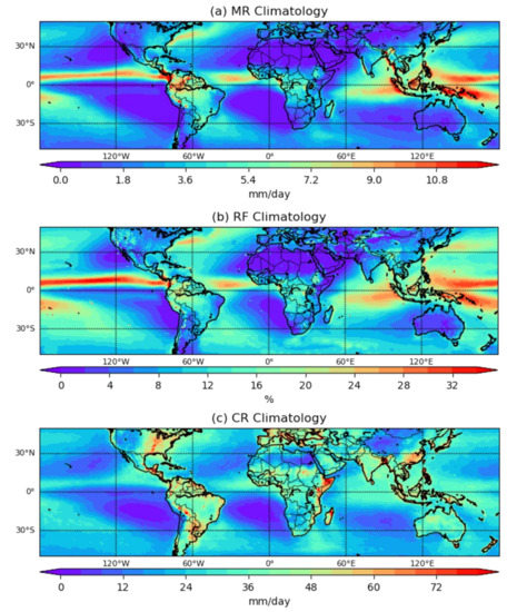
Figure 1.
TMPA climatological (1998–2016) (a) mean precipitation rate (MR), (b) precipitation frequency (RF) and (c) precipitation intensity (CR).
In monsoon climatological areas such as India, Southeast Asia, West African, and Asia–Australia, the RFs are low compared to areas such as upper South America, but CRs in monsoon areas are among the heaviest ones in the world. Monsoons combined with tropical and extratropical cyclones feature prevailing winds and heavy rainfall in wet seasons and low precipitation in dry seasons. There are not abundant numbers of rain events in these areas, but when rains, it usually rains heavily. The shift in the jet stream brings much of the annual precipitation to the east coast of North America [36] and the potential for heavy rainfall events. Therefore, MR, RF, and CR are all high in this area, which are highlighted in all the figures. There are areas which are high in RF but low in CR, such as the western part of America and southeast of the Tibetan Plateau. Desert areas such as the Sahara Desert in North Africa and Taklamakan Desert in West China are also easily distinguishable on the maps, which are low in all the precipitation factors.
Figure 2 shows the timeseries of seasonal anomalies of MR, RF, and CR over the quasi-global scale, and quantitative statistics on the three parameters are carried out in terms of spatiotemporal means, trends of linear regressions, and significance levels as presented in Table 1. A slight but still significant increasing trend (passes 0.05 significance level) can be observed in MR (Figure 2a), while significant decreasing and increasing trends (pass 0.01 significant level) are shown in RF (Figure 2b) and CR (Figure 2c), respectively. The global average MR, RF, and CR through the study period are 2.83 mm/day, 10.55%, and 25.05 mm/day, respectively, in TMPA data, which are comparable with previous studies, such as MR of 2.62 mm/day over 90°N~90°S in the paper of Adler et al. [37] and RF of 11% in the work of Trenberth and Zhang [19].
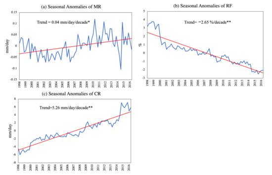
Figure 2.
Anomalies of quasi-global (a) mean precipitation rate (MR), (b) precipitation frequency (RF), and (c) precipitation intensity (CR). * and ** stand for the trend having passed 0.05 and 0.01 significance level, respectively.

Table 1.
Means and trends of the mean rain rate (MR), rain frequency (RF), and conditional rain rate (CR). NH: northern hemisphere; SH: southern hemisphere. Trends without any asterisk have not passed the 0.1 significance level.
Figure 3 shows the seasonal anomalies for the ocean and land over the quasi-global scale and based on the Northern Hemisphere (NH) and Southern Hemisphere (SH). The corresponding statistical and significance test results are generated in Table 1. A hemispheric asymmetry can be observed through the results: the means of all the parameters are higher in the NH than SH for ocean (3.58 mm/day, 13.45%, 23.87 mm/day in the NH vs. 2.50 mm/day, 11.17%, 19.18 mm/day in the SH for MR, RF and CR, respectively) due to the NH-deflection of ITCZ [38]; and inverse phenomena can be observed for land (2.10 mm/day, 5.61%, 34.24 mm/day in the NH vs. 3.29 mm/day, 8.31%, 37.11 mm/day in the SH for MR, RF and CR, respectively) because the maritime continent and Amazon rainforest are mainly distributed in the SH [39,40]. The mean values of MR calculated in this study are comparable to those of GPCP V2.3 (2.95 mm/day for tropical, 3.0 mm/day for ocean, and 2.81 mm/day for land) [37]. As shown in Figure 4, both MR and RF have strong connections with southern oscillation over the land of SH. The correlation coefficients (CC) between them and the Southern Oscillation Index (SOI, one measure of the large-scale fluctuations in air pressure occurring between the western and eastern tropical Pacific during El Niño and La Niña episodes [41]) are 0.72 and 0.65, respectively. There were 74 seasons during our study period and the 95% critical value for CC was +/−0.23 [42]. Thus, it can be confirmed that both MR and RF over SH land are strongly influenced by southern oscillation.
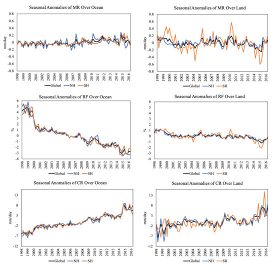
Figure 3.
Anomalies of mean precipitation rate (MR), precipitation frequency (RF) and precipitation intensity (CR) for Ocean (left) and Land (right) in global, northern and southern hemisphere scales.
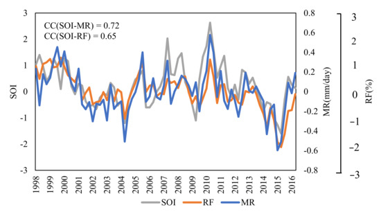
Figure 4.
Correlation between SOI and MR and RF anomalies of land in southern hemisphere.
On the other hand, the ocean has increasing trends in MR for all scopes compared to the decreasing trends over all parts of the land. Although the trends have passed the significant test over ocean and SH land, the absolute values are relatively small (have not exceeded 0.1 mm/day/decade). The trends of RF are decreasing and significant over the ocean and land in all scopes, among which the oceanic ones are more drastic than the terrestrial (~−3.5%/decade vs. ~−0.7%/decade). On the contrary, CR shows significantly increasing trends for all scopes, and it rises faster over the ocean than land through these years (~6 mm/day/decade vs. ~3 mm/day/decade). In addition, the ocean overall has a higher influence on the global precipitation trends than the land. This is due to the existent of regions such as ITCZ and SPCZ over the ocean, where the large scale and huge volume of rainfall is concentrated, while the annual rainfall characteristics over land are more stable with a smaller decreasing trend in RF and increasing trend in CR during the study period. However, the land in general has a larger oscillation among seasons, especially in MR and CR, which indicates a stronger seasonal pattern over land.
Since the precipitation patterns are not identical in different seasons, statistics are also conducted seasonally to obtain the trends in each season; the results are summarized in Table 2. As shown, all the trends in the four seasons have passed the 0.01 significance level except, the MR of the NH spring (March, April, and May, MAM) and NH winter (December, January, and February, DJF), which indicates stable precipitation amounts in these two seasons. Furthermore, although the NH summer (June, July, and August, JJA) presents the largest rainfall amount and highest frequency of rain event, the intensity is not as high as the NH winter and NH autumn (September, October, and November, SON). Moreover, the largest trend of MR appears in the NH autumn; however, the NH summer shows both a sharper decrease in RF and increase in CR.
Table 2.
Seasonal averages and trends of precipitation parameters. Trends without any asterisk have not passed the 0.1 significance level. MAM is short for March, April, and May; JJA is short for June, July, and August; SON is short for September, October, and November, DJF is short for December, January, and February.
3.2. Spatial Patterns of Trends
The spatial patterns of trends are presented in Figure 5. It should be noted that only those trend values that passed the 0.05 significance level are shown. Pixels without significant trends are displayed as invalid (white color). As the global trend map shows, most of the areas do not have significant trends in MR (Figure 5a). However, the northern part of ITCZ as well as some sparse pixels along the edges of storm tracks, SPCZ, and warm currents of the ocean areas show a drastic and significant increasing trend. In addition, the increasing trends can also be observed in South America, the Middle East, and northern China. The pixels with a decreasing trend are mainly located over and near land areas, such as the middle of the USA and the west coastline of South America and Europe. Adler et al. [37] analyzed the spatial trend of the precipitation rate over tropical regions using GPCP data. With similar patterns over regions such as ITCZ, South America, and the Himalayas, they also found widespread positive trends over the Indian Ocean, Maritime Continent, and SPCZ, which cannot be observed in the results of this paper. The differences may potentially be due to different study periods (1970–2017 vs. 1998–2016).
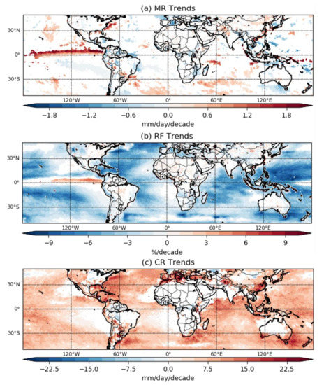
Figure 5.
Spatial patterns of linear trends in (a) MR, (b) RF, and (c) CR during the study period. The values reflect the slope of linear regression at each grid point. Only the trends that pass the 0.05 significance level are shown, which can be consider having a significant trend. Pixels that have no significant trends are shown as invalid (white color).
Figure 5b shows the spatial distribution of the RF trend. It is clear to see that most of the ocean areas show a decreasing trend. Most of the monsoon regions and the dry regions do not show significant trends. Specifically, ocean regions of West Pacific ITCZ, southern China coastline, and center of SPCZ display increasing trends. Unlike the ocean areas that are dominated by the decreasing trend, land in general shows both increasing and decreasing trends.
The spatial pattern of CR is further analyzed, and the result is plotted in Figure 5c. As shown, the vast majority of ocean areas show an obviously increasing trend in CR, except for in a few scattered locations such as (130°W, 10°N), (110°W, 25°N), and (0°,0°). Over land, CR overall has an inverse trend as compared with RF. For example, the rainfall intensity appears to be increasing but the frequency shows a decreasing trend over the western part of the USA and west coast of South America. However, the intensity basically becomes lower, but the frequency becomes higher in the middle of Africa and west of Sahara areas.
In general, significant RF and CR trends are shown in a much wider range than MR. The regions with maximum MR trend are mostly distributed at the maritime continent, which also show significant increasing CRs but a small decreasing trend in RF. This could be attributed to the increase in SST over those regions [43]. It can also be inferred that the precipitation frequency is becoming lower, but the intensity is becoming higher, and the overall global total rainfall is relatively stable over these years, which is consistent with the statistical results listed in Table 1.
3.3. Precipitation Categories Analysis
Figure 6 shows the clustering results (Figure 6a) and the distribution maps (Figure 6b) of precipitation categories over land based on RF and CR. Category 1 is characterized by high RF with a nearly entire range of CR (high frequency, median intensity). Category 2 is featured as the median RF and CR. The precipitation frequency is low in both Category 3 and 4; however, the intensity is much higher in Category 4. The distribution of rainfall categories (Figure 6b) is basically consistent with the global climatological classes [44]. Category 1 is mostly distributed in the tropical wet areas, such as the rain forests of the Amazon and middle of Africa and maritime islands of Southeast Asia. The second type of rainfall mainly appears in mountainous regions, tropical wet and dry areas, such as savannas in Southern America and Africa, as well as part of semiarid and humid continental areas in the USA, China, and India. Category 3 covers most of the arid regions, such as the Sahara, Patagonian, Arabian, Great Victoria, and Gobi deserts. Category 4 mainly appears in humid subtropical and humid continental areas such as the eastern USA, southeast China, and India, and also in the semiarid and arid areas in Australia and Africa. These phenomena prove that the rainfall characteristics of land is influenced by the global climate and determined by the distribution of land cover over the world. Moreover, the climatology of the water cycle is not only related to the total rainfall amount but also to the frequency and intensity.
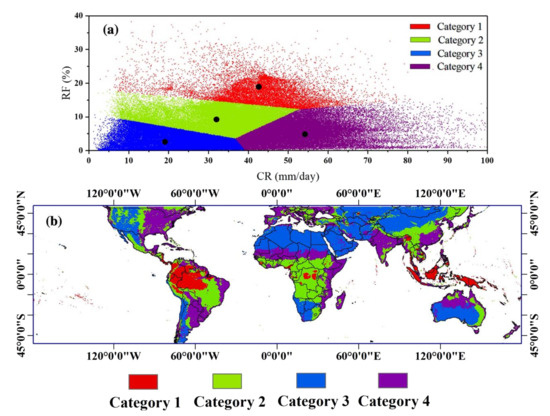
Figure 6.
(a) K-means clustering based on mean RF and CR for land, black dots are the centroids of each cluster. (b) Distributions of precipitation categories over land.
Figure 7 shows the oceanic clustering results (Figure 7a) and the distribution maps of the corresponding categories (Figure 7b). Similar to land, the first category of the ocean is associated with a high intensity and high frequency, and this kind of precipitation is distributed over the ITCZ, SPCZ, and storm tracks such as the eastern coast of the USA. The precipitation of Category 2 covers a major part of the ocean, which is characterized by low intensity and average frequency. The third category refers to the rainfall that is low in both CR and RF. This type appears in the high-pressure cells. The fourth type of rainfall is characterized by high intensity and average frequency, which mainly appears in the coastal and bay areas. These categorization results are basically consistent with the precipitation climatology of the ocean; however, the category with highest intensity and relatively low frequency (Category 4) is not illustrated in the map of the global rainfall amount (MR, Figure 1a). Although the total rainfall amount over these regions is not as high as Category 1, they are usually associated with short-term precipitation extremes that cause huge damage to the economy and to human lives. The clustering results of the ocean can serve as a basis for extreme rainfall detection and prediction along coastal regions to help mitigate loss.
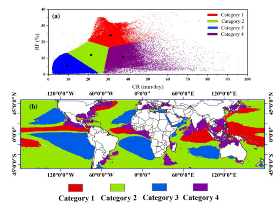
Figure 7.
(a) K-means clustering based on mean RF and CR for ocean, black dots are the centroids of each cluster. (b) Distributions of precipitation categories over ocean.
3.4. Inter-Annual Analysis
A previous study shows that the ENSO has a great influence on the global rainfall amount [45]. In order to further examine its impact on other precipitation parameters, this study investigates the correlations between the first three EOFs of precipitation parameters and ENSO index (Oceanic Niño Index is adopted), and the results are presented in Table 3. The first two EOFs of MR pass the significance test based on the sampling error method [46], and the variances explained are 15.38% and 4.40%, respectively. The EOF1 of MR is characterized by large positive anomalies over ITCZ and is associated with large negative anomalies over the maritime continents, which is interpreted as the strong response to an ENSO pattern. Moreover, its associated time series (PC1) shows a high correlation (CC = −0.93) with the ENSO index [47], indicating that the EOF1 of MR is highly related to ENSO. The dominance of the ENSO in the global rainfall amount is also demonstrated in the spatial pattern of EOF1 and its associated timeseries, which are shown in Figure 8. However, the timeseries of MR does not have a clear correlation with any of the EOFs.
Table 3.
Correlation between first three EOFs of precipitation parameters and seasonal anomalies/ENSO. The coefficients that fall below the 95% critical values of 74 samples (±0.23) are not shown.
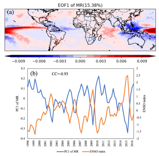
Figure 8.
(a) The first EOF pattern and (b) its associated time series of MR. The variance explained is 15.38%.
All the first three EOFs of RF pass the significance test and explain 34.53%, 9.09%, and 4.39% of the variance, respectively. The first EOF explained more than 30% of the variance, which can be considered distinct and significant. As presented in Figure 9, positive anomalies appear in most areas of EOF1 (Figure 9a), and the texture is almost a reverse of the distribution of RF trends. Furthermore, the associated timeseries also illustrates a decreasing trend that is nearly the same to that of RF (CC = 0.99). These patterns suggest that the RF is determined by its decreasing trend. On the other hand, the second EOF of RF has a high correlation with ENSO (CC = 0.78). Therefore, ENSO is also an important factor that dominates the RF.
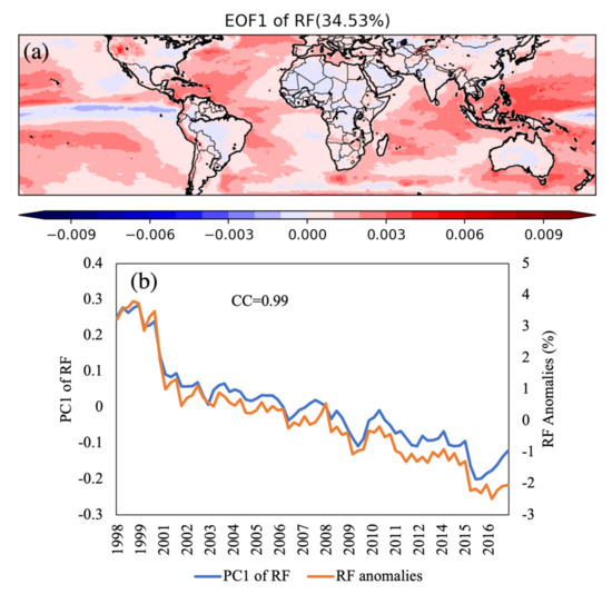
Figure 9.
The same as Figure 8 but for RF. The variance explained is 34.53%. (a) The first EOF pattern and (b) its associated time series of RF.
For CR, only the first EOF passed the significance test, which explained 17.19% of the variance. As shown in Figure 10, the spatial pattern of EOF1 has a similar texture with the distribution of CR trend, and its associated timeseries (PC1) is highly correlated with the seasonal anomalies of CR (CC = −0.99), which indicates that the dominant mode of CR is representative of its trend information.
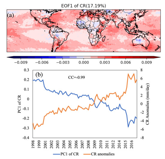
Figure 10.
The same as Figure 8 but for CR. The variance explained is 17.19%. (a) The first EOF pattern and (b) its associated time series of CR.
4. Discussions
This study analyzes the characteristics of the precipitation amount, frequency, and intensity, including their spatiotemporal means, trends, and categories. Overall, the total rainfall amount is determined by both the intensity and frequency. Over land, these characteristics of precipitation parameters are influenced by the global climate, which are evidenced from the consistencies between precipitation categories and climate classifications. Over the ocean, the distributions of rainfall categories are mainly determined by the precipitation climatology of the ocean. However, the characteristics of precipitation parameters and distributions of precipitation types on land are more complex and influenced by more factors such as the topography and prevailing and seasonal winds. For example, over mountainous regions such as the Himalayas, Sierra Madre, the Northern half of the Andes, and the Great Dividing Range, the precipitation is mostly Category 2 with a low CR and median RF. The negative and positive trends in precipitation frequency and density are more significant over the tracks of prevailing wind. The quantitative relations between precipitation and aforementioned factors need to be further examined in our future study. Additionally, although the total rainfall amount over some coastal and bay regions are not as large as that of ITCZ and SPCZ, the intensity is relatively high.
The spatiotemporal mean rainfall rate calculated through this paper is slightly higher than those derived from the study of Yang and Nesbitt [48], which are 2.83, 3.02, and 2.60 mm/day in comparison to 2.46, 2.57, and 2.19 mm/day for quasi-globe, ocean, and land, respectively. The differences can be attributed to the following reasons: the spatial range is different (37.5°N~37.5°S in their paper vs. 50°N~50°S in this paper) and the dataset used in their study utilizes the TRMM precipitation radar (PR) data, which tends to miss the light rainfall, thus underestimating the rainfall amount. Trenberth and Zhang [28] found the rainfall frequency to be 11%, 8.2%, and 12.1% for global scale (60°N~60°S), land, and ocean, respectively, with the CMORPH hourly precipitation rate being greater than or equal to 0.02 mm/h, while these metrics are 10.55%, 6.47%, and 12.15% in this paper. The differences are potentially introduced by the selection of the minimum rain rate criterion, temporal resolution, and spatial scales. We also find that with the decrease in spatiotemporal resolutions, the trends become less significant or even disappear (results are not shown in the paper). Therefore, the analytical results of precipitation trends are sensitive to both the spatiotemporal resolutions of data and criterion of the minimum rain rate. From the spatiotemporal patterns detected in this study, ENSO is found to be the dominant factor that causes the spatiotemporal patterns and variances of global rainfall amount and SOI determines the precipitation in the southern hemisphere.
The paper also finds a significant decreasing trend (−2.65%/decade) in frequency, increasing trend (5.26 mm/day/decade) in intensity, and a small but still significant (passes 0.05 significant level) trend (0.04 mm/day/decade) in the amount for the quasi-global scale of 50°N~50°S. The increase in the global rainfall amount is mainly due to the increase in rainfall in regions such as ITCZ, SPCZ, and storm tracks on the ocean. Overall, the frequency shows decreasing trends, while the intensity shows increasing trends for all scales, indicating that rainfall is becoming more severe over the years and that precipitation extremes have a larger chance of taking place [49]. These trends may also explain the increasing droughts and floods in some areas over these years [50,51]. A recent study carried out by Li et al. [52] achieved an even larger decreasing trend in the precipitation frequency in China with a criterion of 0.1 mm/12h to identify the minimum rainfall rate, which is −5.5%/decade. On the other hand, it is becoming increasingly evident that global warming is contributing to the increasing precipitation intensities and number of extreme rainfalls [53,54], especially as the observed trends are concurrent with a period of significant global warming [55]. The increasing upper ocean heat content caused by solar radiation has a strong link with extreme rainfalls from recent hurricanes [19].
The analysis of different precipitation parameters in this paper provides another dimension of looking at rainfall, not only from the spatiotemporal patterns of amount, but also from the trends, frequency, and intensity. Furthermore, it provides a basis for the calibration and bias-correction of climate models by quantifying the trends. Studies have proved that precipitation extremes over some regions were considerably underrepresented in the model outputs [56], and it can be potentially corrected by introducing the observed trends. However, it is worth noting that the uncertainties of the TRMM 3B42V7 product will cause errors to the analytical results. The microwave (MW) dominant rainfall estimates tend to have more missed detections of precipitation due to how the MW-dominated rain retrieval schemes easily miss light rain from warm and low clouds [57]. Consequently, the actual frequency will be underestimated. The TRMM 3B42V7 product is observed to have a relatively low overall accuracy of ~66% in identifying correct rain and no-rain events over complex topography [58]. The product also suffered from uncertainties caused by orographic convection and the land–ocean classification algorithm [59], which reduced the estimation accuracies over mountainous and coastal regions.
Following the work presented in this paper, future research will focus on the following aspects: (1) conducting sensitivity test on the thresholds of determining rain/no rain in the calculation of frequency and intensity; (2) carrying out separate studies on the analysis of regional precipitations where the parameters show abnormal trends; (3) similar investigations need to be carried out using datasets with different spatiotemporal resolutions to examine if these patterns and trends can be found at other scales; (4) as the TRMM satellite is no longer in operation, but superseded by the GPM satellite, we plan to implement a continuous study using the IMERG dataset to the advantages of its longer availability, higher accuracy, and spatiotemporal resolution [60,61]; (5), including other satellite data, which have a more stable status compared to those adopted in TMPA crossing time variation during the study period; (6) conducting quantitative analysis on the relationship between precipitation patterns and factors such as topography prevailing and seasonal wind, ENSO and SOI.
5. Conclusions
A comprehensive statistical analysis is applied on long-term (18.5 years) TMPA precipitation data at a quasi-global scale (50°N~50°S) with 0.25° and 3-houly spatiotemporal resolutions. Instead of investigating a single parameter in a distinct region, this study focuses on all three factors, namely the amount (MR), frequency (RF), and intensity (CR). We then thoroughly analyzed the results between land and ocean, northern and southern hemisphere, as well as the different seasons. The interannual patterns of all parameters are further investigated and explained using empirical orthogonal function (EOF). This paper also applies K-means clustering technology to the precipitation frequency and intensity to classify the global precipitation into four categories over land and ocean separately. The results of our analysis illustrate new patterns and trends on the combinations of rainfall frequency and intensity, which can be potentially further used in validating and recalibrating the models.
According to the results of experiments and analysis, the paper has the following conclusions:
- (1)
- Globally, the total rainfall amount is higher over ocean than over land, which is accounted by a much higher frequency but a slightly lower intensity over the ocean.
- (2)
- The frequency of rainfall events significantly decreased, while the intensity largely increased over the study period. The precipitation amounts slightly increased due to a combined effect of frequency and intensity. The ocean takes a relatively larger proportion in the global trends of frequency and intensity than land.
- (3)
- The precipitation categories are consistent with the climate classes over land and are mainly determined by oceanic precipitation climatology over the ocean. The clustering results also stand out as some coastal and bay areas do not have the largest rainfall amount but are high in intensity. This information can be useful for precipitation disaster management in these regions.
- (4)
- The total rainfall amount is dominated by the ENSO signal globally, but the frequency and intensity are mostly influenced by their trends in TMPA data. The amount and frequency over the land of the southern hemisphere are also largely influenced by the SOI.
Author Contributions
Conceptualization, Q.L., L.S.C. and C.Y.; writing—original draft preparation, Q.L. and L.S.C.; writing—review and editing, C.Y. and X.H.; funding acquisition, C.Y. and L.S.C. All authors have read and agreed to the published version of the manuscript.
Funding
This research was funded by Ligado Networks (222992), NSF (OAC−1835507 and IIP−1841520), and NASA (NNX15AH51G and NNG14HH38I).
Institutional Review Board Statement
Not applicable.
Informed Consent Statement
Not applicable.
Data Availability Statement
Publicly available datasets were analyzed in this study. These data can be found here: The TRMM data used in this study can be downloaded from NASA’s Goddard Space Flight Center https://pmm.nasa.gov/data-access/downloads/trmm, the data are in these repositories and cited in the references. ENSO indices are obtained from NOAA National Weather Service: https://www.weather.gov/fwd/indices. SOI is downloaded from NOAA National Centers for Environmental Information: https://www.ncdc.noaa.gov/teleconnections/enso/indicators/soi/, (accessed on 15 November 2021).
Acknowledgments
The authors acknowledge Jennifer Smith for helping proofread the paper. This research was funded by Ligado Networks (222992), NSF (OAC−1835507 and IIP−1841520), and NASA (NNX15AH51G and NNG14HH38I).
Conflicts of Interest
The authors declare no conflict of interest.
References
- Xu, H.; Yu, T.; Cheng, T.; Li, J.; Lai, J.; Liu, Q. The research of remote sensing duststorm with FY-3B three infrared channels. In Infrared, Millimeter-Wave, and Terahertz Technologies II; International Society for Optics and Photonics: Bellingham, WA, USA, 2012; Volume 8562, p. 856212. [Google Scholar]
- Xu, H.; Cheng, T.; Gu, X.; Yu, T.; Xie, D.; Zheng, F. Spatiotemporal variability in dust observed over the Sinkiang and Inner Mongolia regions of Northern China. Atmos. Pollut. Res. 2015, 6, 562–571. [Google Scholar] [CrossRef]
- Oldenborgh, G.J.; van der Wiel, K.; Sebastian, A.; Singh, R.; Arrighi, J.; Otto, F.; Cullen, H. Attribution of extreme rainfall from Hurricane Harvey, August 2017. Environ. Res. Lett. 2017, 12, 124009. [Google Scholar] [CrossRef]
- Kawecki, S.; Steiner, A.L. The influence of aerosol hygroscopicity on precipitation intensity during a mesoscale convective event. J. Geophys. Res. Atmos. 2018, 123, 424–442. [Google Scholar] [CrossRef]
- Black, A.W.; Mote, T.L. Characteristics of winter-precipitation-related transportation fatalities in the United States. Weather Clim. Soc. 2015, 7, 133–145. [Google Scholar] [CrossRef]
- Sloat, L.L.; Gerber, J.S.; Samberg, L.H.; Smith, W.K.; Herrero, M.; Ferreira, L.G.; West, P.C. Increasing importance of precipitation variability on global livestock grazing lands. Nat. Clim. Chang. 2018, 8, 214. [Google Scholar] [CrossRef]
- Horn, L.; Hajat, A.; Sheppard, L.; Quinn, C.; Colborn, J.; Zermoglio, M.; Ebi, K. Association between precipitation and diarrheal disease in Mozambique. Int. J. Environ. Res. Public Health 2018, 15, 709. [Google Scholar] [CrossRef] [PubMed]
- Liu, Q.; Harris, J.T.; Chiu, L.S.; Sun, D.; Houser, P.R.; Yu, M.; Duffy, D.Q.; Little, M.M.; Yang, C. Spatiotemporal impacts of COVID-19 on air pollution in California, USA. Sci. Total Environ. 2021, 750, 141592. [Google Scholar] [CrossRef]
- Chiu, L.S.; Gao, S.; Shin, D.-B. Climate-Scale Oceanic Rainfall Based on Passive Microwave Radiometry. In Satellite-Based Applications on Climate Change; Qu, J., Ed.; Springer: New York, NY, USA, 2013; pp. 225–245. [Google Scholar]
- Carson, M.; Lyu, K.; Richter, K.; Becker, M.; Domingues, C.M.; Han, W.; Zanna, L. Climate model uncertainty and trend detection in regional sea level projections: A review. Surv. Geophys. 2019, 40, 1631–1653. [Google Scholar] [CrossRef]
- Donat, M.G.; Lowry, A.L.; Alexander, L.V.; O’Gorman, P.A.; Maher, N. More extreme precipitation in the world’s dry and wet regions. Nat. Clim. Chang. 2016, 6, 508. [Google Scholar] [CrossRef]
- Valdes-Abellan, J.; Pardo, M.A.; Tenza-Abril, A.J. Observed precipitation trend changes in the western Mediterranean region. Int. J. Climatol. 2017, 37, 1285–1296. [Google Scholar] [CrossRef]
- Trenberth, K.E. Conceptual Framework for Changes of Extremes of the Hydrological Cycle with Climate Change. Limatic Chang. 1999, 42, 327–339. [Google Scholar] [CrossRef]
- Jakob, C.; Schumacher, C. Precipitation and Latent Heating Characteristics of the Major Tropical Western Pacific Cloud Regimes. J. Clim. 2007, 21, 4348–4364. [Google Scholar] [CrossRef]
- Pendergrass, A.G.; Hartmann, D.L. Changes in the Distribution of Rain Frequency and Intensity in Response to Global Warming. J. Clim. 2014, 27, 8372–8383. [Google Scholar] [CrossRef]
- Adler, R.F.; Gu, G.; Sapiano, M.; Wang, J.-J.; Huffman, G.J. Global Precipitation: Means, Variations and Trends During the Satellite Era (1979–2014). Surv. Geophys. 2017, 38, 679–699. [Google Scholar] [CrossRef]
- Gu, G.; Adler, R.F. Precipitation intensity changes in the tropics from observations and models. J. Clim. 2018, 31, 4775–4790. [Google Scholar] [CrossRef]
- Shang, H.; Xu, M.; Zhao, F.; Tijjani, S.B. Spatial and Temporal Variations in Precipitation Amount, Frequency, Intensity, and Persistence in China, 1973–2016. J. Hydrometeorol. 2019, 20, 2215–2227. [Google Scholar] [CrossRef]
- Trenberth, K.E.; Zhang, Y. Near-Global Covariability of Hourly Precipitation in Space and Time. J. Hydrometeorol. 2018, 19, 695–713. [Google Scholar] [CrossRef]
- Miao, C.; Duan, Q.; Sun, Q.; Lei, X.; Li, H. Non-uniform changes in different categories of precipitation intensity across China and the associated large-scale circulations. Environ. Res. Lett. 2018, 14, 025004. [Google Scholar] [CrossRef]
- GES DISC. TRMM (TMPA) Rainfall Estimate L3 3 Hour 0.25 Degree x 0.25 Degree V7, Greenbelt, MD, Goddard Earth Sciences Data and Information Services Center (GES DISC). 2011. Available online: https://disc.gsfc.nasa.gov/ (accessed on 8 April 2017).
- Kummerow, C.; Barnes, W.; Kozu, T.; Shiue, J.; Simpson, J. The tropical rainfall measuring mission (TRMM) sensor package. J. Atmos. Ocean. Technol. 1998, 15, 809–817. [Google Scholar] [CrossRef]
- Yu, Z.; Yu, H.; Chen, P.; Qian, C.; Yue, C. Verification of tropical cyclone—Related satellite precipitation estimates in mainland China. J. Appl. Meteorol. Climatol. 2009, 48, 2227–2241. [Google Scholar] [CrossRef]
- Sahoo, A.K.; Sheffield, J.; Pan, M.; Wood, E.F. Evaluation of the tropical rainfall measuring mission multi-satellite precipitation analysis (TMPA) for assessment of large-scale meteorological drought. Remote Sens. Environ. 2015, 159, 181–193. [Google Scholar] [CrossRef]
- Nguyen, P.; Ombadi, M.; Sorooshian, S.; Hsu, K.; AghaKouchak, A.; Braithwaite, D.; Ashouri, H.; Thorstensen, A.R. The PERSIANN family of global satellite precipitation data: A review and evaluation of products. Hydrol. Earth Syst. Sci. 2018, 22, 5801–5816. [Google Scholar] [CrossRef]
- Huffman, G.J.; Adler, R.F.; Bolvin, D.T.; Nelkin, E.J. The TRMM Multi-Satellite Precipitation Analysis (TMPA). In Satellite Rainfall Applications for Surface Hydrology; Springer: Dordrecht, The Netherlands, 2010; pp. 3–22. [Google Scholar]
- Karbalaee, N.; Hsu, K.; Sorooshian, S.; Braithwaite, D. Bias adjustment of infrared-based rainfall estimation using passive microwave satellite rainfall data. J. Geophys. Res. Atmos. 2017, 122, 3859–3876. [Google Scholar] [CrossRef]
- Trenberth, K.E.; Zhang, Y. How often does it really rain? BAMS 2017, 99, 289–298. [Google Scholar] [CrossRef]
- Liu, Q.; Chiu, L.S.; Hao, X. The Impact of Spatial and Temporal Resolutions in Tropical Summer Rainfall Distribution: Preliminary Results. ISPRS Ann. Photogramm. Remote Sens. Spat. Inf. Sci. 2017, 4, 183. [Google Scholar] [CrossRef]
- Chen, D.; Dai, A. Dependence of estimated precipitation frequency and intensity on data resolution. Clim. Dyn. 2018, 50, 3625–3647. [Google Scholar] [CrossRef]
- Blamey, R.C.; Reason, C.J.C. The role of mesoscale convective complexes in southern Africa summer rainfall. J. Clim. 2013, 26, 1654–1668. [Google Scholar] [CrossRef]
- Zahra, S.; Ghazanfar, M.A.; Khalid, A.; Azam, M.A.; Naeem, U.; Prugel-Bennett, A. Novel centroid selection approaches for KMeans-clustering based recommender systems. Inf. Sci. 2015, 320, 156–189. [Google Scholar] [CrossRef]
- Von Storch, H.; Zwiers, F.W. Statistical Analysis in Climate Research; Cambridge University Press: Cambridge, UK, 2001. [Google Scholar]
- Liu, Z. Comparison of Integrated Multisatellite Retrievals for GPM (IMERG) and TRMM Multisatellite Precipitation Analysis (TMPA) Monthly Precipitation Products: Initial Results. J. Hydrometeorol. 2016, 17, 777–790. [Google Scholar] [CrossRef]
- Venugopal, V.; Wallace, J.M. Climatology of contribution-weighted tropical rain rates based on TRMM 3B42. Geophys. Res. Lett. 2016, 43, 10439–10447. [Google Scholar] [CrossRef]
- Marciano, C.G.; Lackmann, G.M.; Robinson, W.A. Changes in US East Coast cyclone dynamics with climate change. J. Clim. 2015, 28, 468–484. [Google Scholar] [CrossRef]
- Adler, R.F.; Sapiano, M.R.; Huffman, G.J.; Wang, J.-J.; Gu, G.; Bolvin, D.; Shin, D.-B. The Global Precipitation Climatology Project (GPCP) Monthly Analysis (New Version 2.3) and a Review of 2017 Global Precipitation. Atmosphere 2018, 9, 138. [Google Scholar] [CrossRef]
- Lashkari, H.; Mohammadi, Z.; Keikhosravi, G. Annual fluctuations and displacements of inter tropical convergence zone (ITCZ) within the range of Atlantic Ocean-India. Open J. Ecol. 2017, 7, 12–33. [Google Scholar] [CrossRef]
- Jaramillo, L.; Poveda, G.; Mejía, J.F. Mesoscale convective systems and other precipitation features over the tropical Americas and surrounding seas as seen by TRMM. Int. J. Climatol. 2017, 37, 380–397. [Google Scholar] [CrossRef]
- Tan, H.; Ray, P.; Barrett, B.; Dudhia, J.; Moncrieff, M.W. Systematic patterns in land precipitation due to convection in neighboring islands in the Maritime Continent during MJO propagation. J. Geophys. Res. Atmos. 2021, 126, e2020JD033465. [Google Scholar] [CrossRef]
- NOAA. Southern Oscillation Index (SOI). Retrieved 19 April 2021, from National Centers for Environmental Information; 2016. Available online: https://www.ncdc.noaa.gov/teleconnections/enso/indicators/soi/ (accessed on 22 August 2019).
- Rohlf, F.J.; Sokal, R.R. Statistical Tables; Macmillan: New York, NY, USA, 1995. [Google Scholar]
- McBride, J.L.; Haylock, M.R.; Nicholls, N. Relationships between the Maritime Continent heat source and the El Niño–Southern Oscillation phenomenon. J. Clim. 2003, 16, 2905–2914. [Google Scholar] [CrossRef]
- Beck, H.E.; Zimmermann, N.E.; McVicar, T.R.; Vergopolan, N.; Berg, A.; Wood, E.F. Present and future Köppen-Geiger climate classification maps at 1-km resolution. Sci. Data 2018, 214, 1–12. [Google Scholar] [CrossRef] [PubMed]
- Henderson, D.S.; Kummerow, C.D.; Berg, W. ENSO influence on TRMM tropical oceanic precipitation characteristics and rain rates. J. Clim. 2018, 31, 3979–3998. [Google Scholar] [CrossRef]
- North, G.R.; Bell, T.L.; Cahalan, R.F.; Moeng, F.J. Sampling Errors in the Estimation of Empirical Orthogonal Functions. Mon. Weather Rev. 1982, 110, 699–705. [Google Scholar] [CrossRef]
- Sun, Q.; Miao, C.; Duan, Q.; Ashouri, H.; Sorooshian, S.; Hsu, K.-L. A Review of Global Precipitation Data Sets: Data Sources, Estimation, and Intercomparisons. Rev. Geophys. 2018, 56, 79–107. [Google Scholar] [CrossRef]
- Yang, S.; Nesbitt, S.W. Statistical properties of precipitation as observed by the TRMM precipitation radar. Geophys. Res. Lett. 2014, 41, 5636–5643. [Google Scholar] [CrossRef]
- Mukherjee, S.; Aadhar, S.; Stone, D.; Mishra, V. Increase in extreme precipitation events under anthropogenic warming in India. Weather Clim. Extrem. 2018, 20, 45–53. [Google Scholar] [CrossRef]
- Güner Bacanli, Ü. Trend analysis of precipitation and drought in the A egean region, Turkey. Meteorol. Appl. 2017, 24, 239–249. [Google Scholar] [CrossRef]
- Bartiko, D.; Oliveira, D.Y.; Bonumá, N.B.; Chaffe, P.L.B. Spatial and seasonal patterns of flood change across Brazil. Hydrol. Sci. J. 2019, 64, 1071–1079. [Google Scholar] [CrossRef]
- Li, Y.; Guo, B.; Wang, K.; Wu, G.; Shi, C. Performance of TRMM Product in Quantifying Frequency and Intensity of Precipitation during Daytime and Nighttime across China. Remote Sens. 2020, 12, 740. [Google Scholar] [CrossRef]
- Fischer, E.M.; Knutti, R. Anthropogenic contribution to global occurrence of heavy-precipitation and high-temperature extremes. Nat. Clim. Chang. 2015, 5, 560. [Google Scholar] [CrossRef]
- Liu, Q.; Li, Y.; Yu, M.; Chiu, L.S.; Hao, X.; Duffy, D.Q.; Yang, C. Daytime Rainy Cloud Detection and Convective Precipitation Delineation Based on a Deep Neural Network Method Using GOES-16 ABI Images. Remote Sens. 2019, 11, 2555. [Google Scholar] [CrossRef]
- Field, C.B.; Barros, V.R. (Eds.) Climate Change 2014–Impacts, Adaptation and Vulnerability: Regional Aspects; Cambridge University Press: Cambridge, UK, 2014. [Google Scholar]
- Bannister, D.; Orr, A.; Jain, S.K.; Holman, I.P.; Momblanch, A.; Phillips, T.; Adeloye, A.J.; Snapir, B.; Waine, T.W.; Hosking, J.S.; et al. Bias correction of high-resolution regional climate model precipitation output gives the best estimates of precipitation in Himalayan catchments. J. Geophys. Res. Atmos. 2019, 124, 14220–14239. [Google Scholar] [CrossRef]
- Rauniyar, S.P.; Protat, A.; Kanamori, H. Uncertainties in TRMM-Era multisatellite-based tropical rainfall estimates over the Maritime Continent. Earth Space Sci. 2017, 4, 275–302. [Google Scholar] [CrossRef]
- Bharti, V.; Singh, C. Evaluation of error in TRMM 3B42V7 precipitation estimates over the Himalayan region. J. Geophys. Res. Atmos. 2015, 120, 12458–12473. [Google Scholar] [CrossRef]
- Kim, K.; Park, J.; Baik, J.; Choi, M. Evaluation of topographical and seasonal feature using GPM IMERG and TRMM 3B42 over Far-East Asia. Atmos. Res. 2017, 187, 95–105. [Google Scholar] [CrossRef]
- Chen, F.; Li, X. Evaluation of IMERG and TRMM 3B43 monthly precipitation products over mainland China. Remote Sens. 2016, 8, 472. [Google Scholar] [CrossRef]
- Fang, J.; Yang, W.; Luan, Y.; Du, J.; Lin, A.; Zhao, L. Evaluation of the TRMM 3B42 and GPM IMERG products for extreme precipitation analysis over China. Atmos. Res. 2019, 223, 24–38. [Google Scholar] [CrossRef]


Publisher’s Note: MDPI stays neutral with regard to jurisdictional claims in published maps and institutional affiliations. |
© 2021 by the authors. Licensee MDPI, Basel, Switzerland. This article is an open access article distributed under the terms and conditions of the Creative Commons Attribution (CC BY) license (https://creativecommons.org/licenses/by/4.0/).