Article

Quantification of Wide-Area Norwegian Spring-Spawning Herring Population Density with Ocean Acoustic Waveguide Remote Sensing (OAWRS)

1
Massachusetts Institute of Technology, 77 Massachusetts Avenue, Cambridge, MA 02139, USA
2
Institute of Marine Research, Post Office Box 1870, Nordnes, N-5817 Bergen, Norway
*
Author to whom correspondence should be addressed.
Remote Sens. 2021, 13(22), 4546; https://doi.org/10.3390/rs13224546
Submission received: 18 August 2021 / Revised: 30 October 2021 / Accepted: 9 November 2021 / Published: 12 November 2021
(This article belongs to the Section Ocean Remote Sensing)

Abstract

:
Norwegian spring-spawning herring are a critical economic resource for multiple nations in the North Atlantic and a keystone species of the Nordic Seas ecosystem. Given the wide areas that the herring occupy, it is difficult to accurately measure the population size and spatial distribution. Ocean Acoustic Waveguide Remote Sensing (OAWRS) was used to instantaneously measure the areal population density of Norwegian herring over more than one thousand square kilometers in spawning grounds near Ålesund, Norway. In the vicinity of the Ålesund trench near peak spawning, significant attenuation in signal-to-noise ratio and mean sensing range was observed after nautical sunset that had not been observed in previous OAWRS surveys in the Nordic Seas or in other regions. We show that this range-dependent decay along a given propagation path was caused by attenuation through dense herring shoals forming at sunset and persisting through the evening for transmissions near the swimbladder resonance peak. OAWRS transmissions are corrected for attenuation in a manner consistent with waveguide scattering theory and simultaneous downward directed local line-transect measurements in the region in order to produce instantaneous wide-area population density maps. Corresponding measured reductions in the median sensing range over the azimuth before ambient noise limitation are shown to be theoretically predictable from waveguide scattering theory and observed population densities. Spatial-temporal inhomogeneities in wide-area herring distributions seen synoptically in OAWRS imagery show that standard sparsely spaced line-transect surveys through this region during spawning can lead to large errors in the estimated population due to spatial and temporal undersampling.

1. Introduction

Norwegian spring-spawning herring is a critical economic resource for multiple nations in the North Atlantic. Since 2013, disagreements over the shifting spatial distribution of this herring stock have prevented these nations from negotiating quota sharing agreements, resulting in a combined catch exceeding the recommended limit by more than 30% in the past three years [1]. It is therefore important to accurately measure the population size and spatial distribution for Norwegian herring over ecosystem scales. Oceanic fish groups, however, occupy vast undersea areas that are difficult to sample without significant aliasing in space and time with conventional survey methods [2,3].
Here, we demonstrate the ability of Ocean Acoustic Waveguide Remote Sensing (OAWRS) to instantaneously image Norwegian herring shoals over more than one thousand square kilometers in spawning grounds near Ålesund, Norway. Wide-area OAWRS scattering strength maps are generated by correcting transmissions for source level and areal resolution footprint, as well as transmission losses from spreading and seafloor attenuation [4,5,6,7,8].
Previous OAWRS experiments have revealed the diel shoaling patterns of massive fish groups, including vertical migrations of shoaling herring measured from changes in the resonance frequency of the fish as they move from deep water to their spawning locations [9]. OAWRS also revealed that shoaling fish tend to rapidly congregate in massive groups spanning tens of kilometers when the fish population density reaches a species-specific critical value [4]. Shoal growth was found to propagate horizontally outward in compressional waves at speeds orders of magnitude larger than the swimming speed of a fish, indicating that shoal formation is the result of synchronous convergence of individual fish [4,5].
These massive fish groups are found to have a relatively stable mean size, and historical population surveys have shown that when a given species was overfished to the point where the total spawning population fell within a standard deviation of the group size a return to pre-industrial total spawning populations took decades [10]. OAWRS has also been used to observe ecosystem-scale interactions between fish groups and marine mammals that forage for fish, and it was shown that marine mammals will spatially converge on fish spawning grounds and divide into separate foraging areas specific to each marine mammal species [11].
Here, OAWRS is used to investigate the effects of diel shoaling behavior of fish groups on acoustic sensing in the ocean. During the day, the OAWRS system revealed small, dispersed groups of herring in the Ålesund spawning grounds with dimensions that were typically less than 1 km. After nautical sunset, the formation of numerous dense herring groups was observed, corresponding with a significant range-dependent decay in OAWRS imagery even after making typical corrections for spreading loss and seafloor attenuation.
This range-dependent decay can be explained by acoustic attenuation through the dense herring groups. Such attenuation requires exceptionally high fish population densities over significant portions of the water column and extended ranges [12] and thus was not observed previously in OAWRS fish sensing, including Mid-Atlantic Bight herring [5], Gulf of Maine herring [6] and Lofoten cod [10]. Reductions in the ambient noise level after nautical sunset can be similarly explained by attenuation from the herring groups.
The organization of this paper is as follows: wide-area OAWRS maps of herring population density are presented, and range-dependent decays in OAWRS transmissions are corrected with a theoretical formulation that was previously shown to be consistent with experimental measurements of attenuation from fish in a waveguide environment [12,13]. Formulations are then introduced for predicting ambient noise reductions and sensing range reductions due to attenuation from fish. The predicted reductions in ambient noise are shown to be theoretically consistent with the measured reductions when dense herring shoals form after nautical sunset.
Theoretical predictions of sensing range are confirmed using measurements of OAWRS sensing range in the presence of herring in Ålesund spawning grounds, capelin in Finnmark spawning grounds, and cod in Lofoten spawning spawning grounds. Spatial-temporal inhomogeneities in wide-area herring distributions observed by OAWRS indicate that significant errors are expected in sparse temporal-spatial line transect surveys through this region during spawning. Equivalent echosounder measurements of the herring population, for example, are estimated by sampling 2014 spatially continuous OAWRS wide-area population density data with the sparse line-transects of a 2001 herring survey in the same region.

2. Methods and Materials

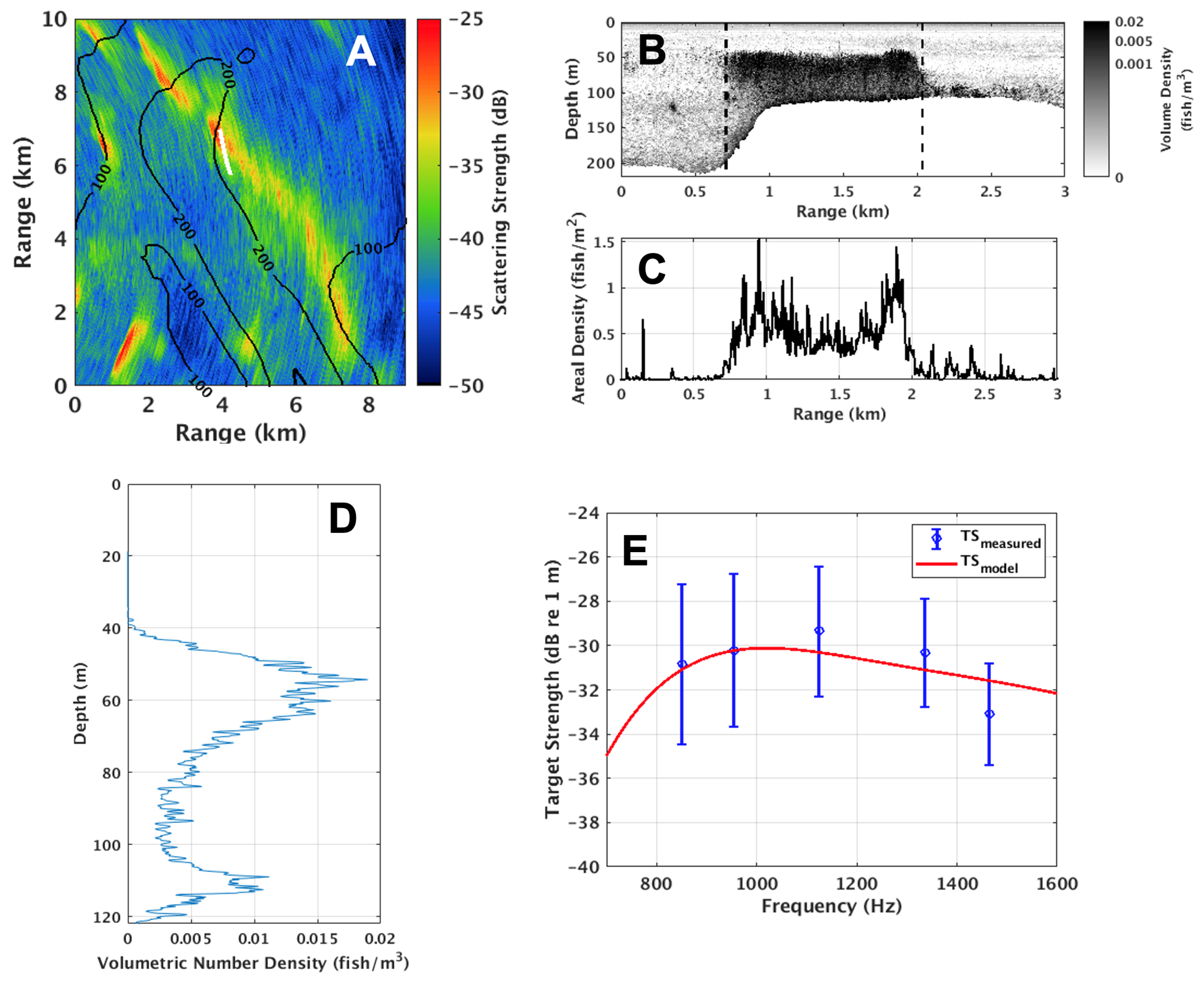
2.1. Population Density Measurements without Significant Fish-Attenuation

Ocean Acoustic Waveguide Remote Sensing (OAWRS) is used to instantaneously monitor Norwegian herring spawning grounds over more than one thousand square kilometers off the coast of Ålesund, Norway (Figure 1). OAWRS sound pressure level maps are generated by beamforming, matched filtering and charting scattered returns [4,5,6,7,8]. Scattering strength levels are determined by correcting sound pressure level maps for source level, areal resolution footprint, spreading loss and seafloor attenuation [4,5,6,7] (Appendix A).
Approximately one hour before nautical sunset, the OAWRS system reveals small, dispersed groups of herring with dimensions that are typically less than 1 km (Figure 2A), and there are few herring groups observed in echosounder measurements from the research vessel towing the OAWRS system (Figure 2B). Scattering strength is converted to areal population density by calibration with local in situ measurements of population density obtained from vertical echosounder measurements (Appendix B), and the dispersed herring groups are found to have population densities on the order of 0.3 fish/m2 (Figure 3).
During this time, the median sensing range over azimuth for the OAWRS system is approximately 20 km, where the sensing range is defined as the minimum range where scattered returns from the environment fall within the detection threshold of the ambient noise (Appendix C). Attempts to measure scattering strength beyond the sensing range limit where ambient noise dominates will not lead to an actual scattering strength but to a quantity that increases with range since transmission loss corrections are being applied to ambient noise with relatively constant mean intensity over time unless it is dominated by a particular nearby ship or sound source.

2.2. Correcting Population Density Maps for Fish-Attenuation

On the same day and in the same region as the daylight measurements of Figure 2 and Figure 3, there is a significant range-dependent decay in the intensity of OAWRS transmissions after sunset, even after making the same standard corrections as in Figure 2 for source level, areal resolution footprint, spreading loss, and seafloor attenuation (Figure 4). This range-dependent decay can be explained by acoustic attenuation from dense herring groups forming at sunset, which are observed in both OAWRS imagery and echosounder measurements from the research vessel towing the OAWRS system.
OAWRS images are corrected for attenuation from fish scattering using a theoretical formulation that has been previously shown to be consistent with experimental measurements of attenuation from fish in a waveguide (Appendix D) [12,13] (Figure 5). The theoretical decay due to attenuation depends on the average population density of fish within the sensing region n ¯ A , which is estimated by modeling the fish-attenuated scattering strength ( S S ˜ S S Δ S P L 2 w a y ) assuming a horizontally uniform distribution of fish within the OAWRS sensing region and performing a least-squares fit between the measured and modeled fish-attenuated scattering strength.
Measurements of the mean fish-attenuated scattering strength ( S S ˜ d a t a ) with respect to range ρ are calculated by correcting OAWRS sound pressure level maps for source level, areal resolution footprint, spreading loss and seafloor attenuation according to Equation (A4), and then averaging across azimuthal angle excluding beams within 25° of endfire. The modeled fish-attenuated scattering strength ( S S ˜ m o d e l ) at range ρ and assuming average areal density n ¯ A is given by:
S S ˜ m o d e l ( n ¯ A , ρ ) 10 log 10 10 S S f i s h ( n A ) / 10 + 10 S S s e a f l o o r / 10 Δ S P L 2 w a y , m o d e l ( n A , ρ )
where S S s e a f l o o r = 43 dB is the measured scattering strength of seafloor in the region, and S S f i s h is the scattering strength of the fish groups, given [7] by:
S S f i s h ( n A ) = T S + 10 log 10 ( n A )
where T S is the target strength of an individual fish (Appendix E) and Δ S P L 2 w a y , m o d e l is the predicted reduction in sound pressure level caused by attenuation from fish (Equation (A15)), which is modeled assuming the depth distribution of herring groups measured by echosounders during this time (Figure A6).
The average areal density of the herring within the sensing region of the OAWRS system is determined using a least-square estimation performed by maximizing the likelihood function. Since the acoustic field can be described as a circular complex Gaussian random variable (CCGR) and the time-bandwidth product of the acoustic measurements μ = ( 1 s ) ( 50 Hz ) 1 , intensity measurements in the logarithmic domain, such as the fish-attenuated scattering strength, can be well-approximated as Gaussian random variables with variance independent of the mean [14,15]. The mean herring areal density is estimated by maximizing the log-likelihood function ( n ¯ A ) assuming that fish-attenuated scattering strength S S ˜ is a Gaussian random variable with variance independent of the mean:
( n ¯ A ) = ρ m i n ρ s e n s S S ˜ m o d e l ( n ¯ A , ρ ) S S ˜ d a t a ( ρ ) 2 σ S S ˜ ( ρ ) 2 ρ d ρ
where σ S S ˜ ( ρ ) 2 is the variance of S S ˜ d a t a in dB at range ρ , and the differential ρ d ρ is chosen in order to integrate over range in polar coordinates. Since the log-likelihood function is calculated by integrating the weighted difference squared across range in polar coordinates, measurements at longer ranges are weighted more heavily since they correspond to a larger area.
The minimum range ρ m i n = 2 km is chosen so that acoustic data is only considered at ranges well above farfield ρ > L 2 / λ , where L = 47.25 is the length of the receiver array [16] and λ = 1.57 m is the acoustic wavelength at the sensing frequency 955 Hz. The sensing range ρ s e n s is defined in Section 2.4. Once the average areal density n ¯ A is determined for a given OAWRS transmission, a range-dependent correction can be applied to scattering strength maps at each azimuthal angle according to:
S S ( ρ , θ ) = S S ˜ d a t a ( ρ , θ ) + Δ S P L 2 w a y ( n ¯ A , ρ )
This method is used to produce herring population density maps after nautical sunset where attenuation is significant (Figure 6). Multiple large herring groups are observed after sunset with dimensions of several kilometers and population densities of up to roughly five fish/m2, which is consistent with echosounder measurements during this time (Figure A5).

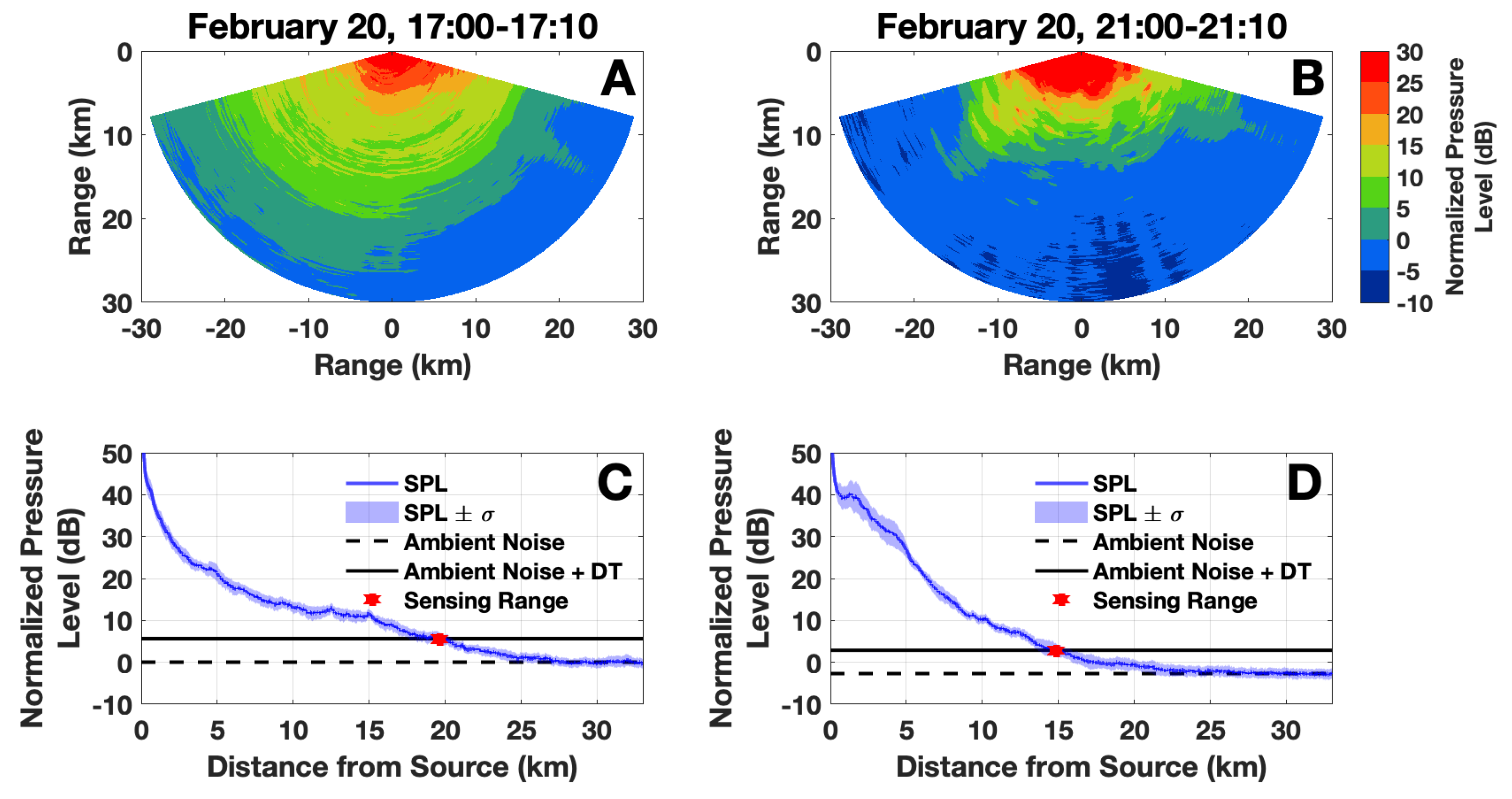
2.3. Predicting Ambient Noise Reductions from Fish-Attenuation

Reductions in the ambient noise level are observed after nautical sunset (Figure 7A), and they can be explained by attenuation from herring groups. Here, a formulation is introduced for predicting reductions in the ambient noise levels due to attenuation from fish. Since the dominant source of ambient noise is assumed to be surface waves, ambient noise is modeled as coming from a uniform set of uncorrelated monopoles at the surface. The intensity of the ambient noise field in a shallow water environment is then given [17] by:
I = 8 π 2 q 2 k 2 0 ξ g ( ξ ; z , z 0 ) d ξ
where k is the wavenumber, q is the amplitude of an individual monopole at depth z 0 near the surface, and g ( ξ ; z , z 0 ) is the wavenumber-depth Green function for horizontal wavenumber ξ and receiver depth z, which can be written in a waveguide environment in terms of normal modes [17] as follows:
g ( ξ ; z , z 0 ) = d 2 π n u n ( z ) u n ( z 0 ) ξ 2 ξ n 2
where ξ n is the modal horizontal wavenumber, d is water density, and the amplitude of mode n at receiver depth z is given by u n ( z ) .
In order for the integral in Equation (5) to converge, some attenuation must be included in the system. This is because the signal from each monopole suffers cylindrical spreading loss, but the energy radiated by the monopoles increases with the range from the receiver squared [17]. Environmental attenuation (not including attenuation from fish) is introduced by letting the wavenumber k be complex:
k = 2 π f c + i ϵ
where f is the frequency, c is the speed of sound in water, and ϵ is a coefficient for environmental attenuation excluding fish [17,18]. The modal wavenumbers ( ξ n ) are also assumed to be complex, with the form:
ξ n = κ n + i α n
where the modal attenuation coefficient α n is given [19] by
α n = ϵ κ n 0 D 2 π f c ( z ) u n ( z ) 2 d z
where D is the water depth. In the absence of attenuation from fish, the ambient field can then be written [17] as:
I = π q 2 d 2 2 k 2 n u n ( z ) 2 u n ( z 0 ) 2 κ n α n
In the presence of fish, the modal wavenumber equation is modified to include the modal coefficients for attenuation and dispersion from fish ( ν n ):
ξ n = κ n + i α n + ν n ( n A ) = ( κ n + [ ν n ( n A ) ] ) + i ( α n + [ ν n ( n A ) ] )
where ν n ( n A ) is defined in Equation (A22). Following the same derivation that led to Equation (10), the ambient noise field in the presence of attenuation from fish can be written as:
I a t t n ( n A ) = π q 2 d 2 2 k 2 n u n ( z ) 2 u n ( z 0 ) 2 ( κ n + [ ν n ( n A ) ] ) ( α n + [ ν n ( n A ) ] )
The decrease in the ambient noise level from attenuation as fish density increases from n A 1 to n A 2 can then be given by:
Δ N L p a r t i a l ( n A 1 , n A 2 ) = 10 log 10 I a t t n ( n A 1 ) I a t t n ( n A 2 ) = 10 log 10 [ n u n ( z ) 2 u n ( z 0 ) 2 ( κ n + [ ν n ( n A 1 ) ] ) ( α n + [ ν n ( n A 1 ) ] ) n u n ( z ) 2 u n ( z 0 ) 2 ( κ n + [ ν n ( n A 2 ) ] ) ( α n + [ ν n ( n A 2 ) ] ) 1 ]
where n A 1 < n A 2 .

2.4. Predicting Sensing Range Reductions from Fish-Attenuation

The observed reductions in signal intensity and ambient noise due to attenuation from fish can contribute to fluctuations in the sensing range for long-range active acoustic sensing systems in the ocean. Here, a formulation is introduced for predicting sensing range in the presence of attenuation from fish. The sensing range ( ρ s e n s ) is defined as:
ρ s e n s ( f , n A ) = min [ ρ | S P L A ( ρ , f , n A ) > N L ( f ) Δ N L ( f , n A ) + D T ]
where S P L A is the azimuthally intensity-averaged sound-pressure level of the received signal, N L is the ambient noise level, D T is the detection threshold, f is the sensing frequency, and it is assumed that fish are uniformly distributed in the horizontal within the sensing region with average areal density n A . Ambient noise level N L is determined from measurements before nautical sunset (17:00–18:30 on 20 February) in order to avoid attenuation effects caused by the formation of herring groups after nautical sunset (Figure 7A). The reduction in ambient noise due to attenuation from fish ( Δ N L ) is modeled according to Section 2.3. The azimuthally intensity-averaged sound-pressure level S P L A is estimated by averaging the intensity of the scattered field across the azimuthal angle θ :
S P L A ( ρ , f , n A ) = 10 log 10 1 θ m a x θ m i n θ m i n θ m a x Ψ ( ρ , f , n A , θ ) Ψ r e f 2 d θ
where Ψ ( ρ , f , n A , θ ) is the modeled scattered field, Ψ r e f = 1   μ Pa is the reference pressure for underwater sound, and the limits of integration θ m i n and θ m a x are chosen to exclude beams within 25° of endfire. Assuming that scattered returns from the environment are dominated by scattering from fish groups rather than seafloor scattering, the intensity of the scattered field Ψ ( ρ , f , n A , θ ) Ψ r e f 2 is modeled according [12] to
10 log 10 Ψ ( ρ , f , n A , θ ) Ψ r e f 2 = S L + T L A ( ρ , f , θ ) + T S ( f ) + 10 log 10 ( n A ) Δ S P L 2 w a y ( ρ , f , n A )
Transmission loss area T L A is calculated according to Equation (A2). The formulation for target strength T S is shown in Appendix E and the formulation for the decrease in sound pressure level during two-way propagation due to the attenuation from fish ( Δ S P L 2 w a y ) is shown in Equation (A15).

3. Results

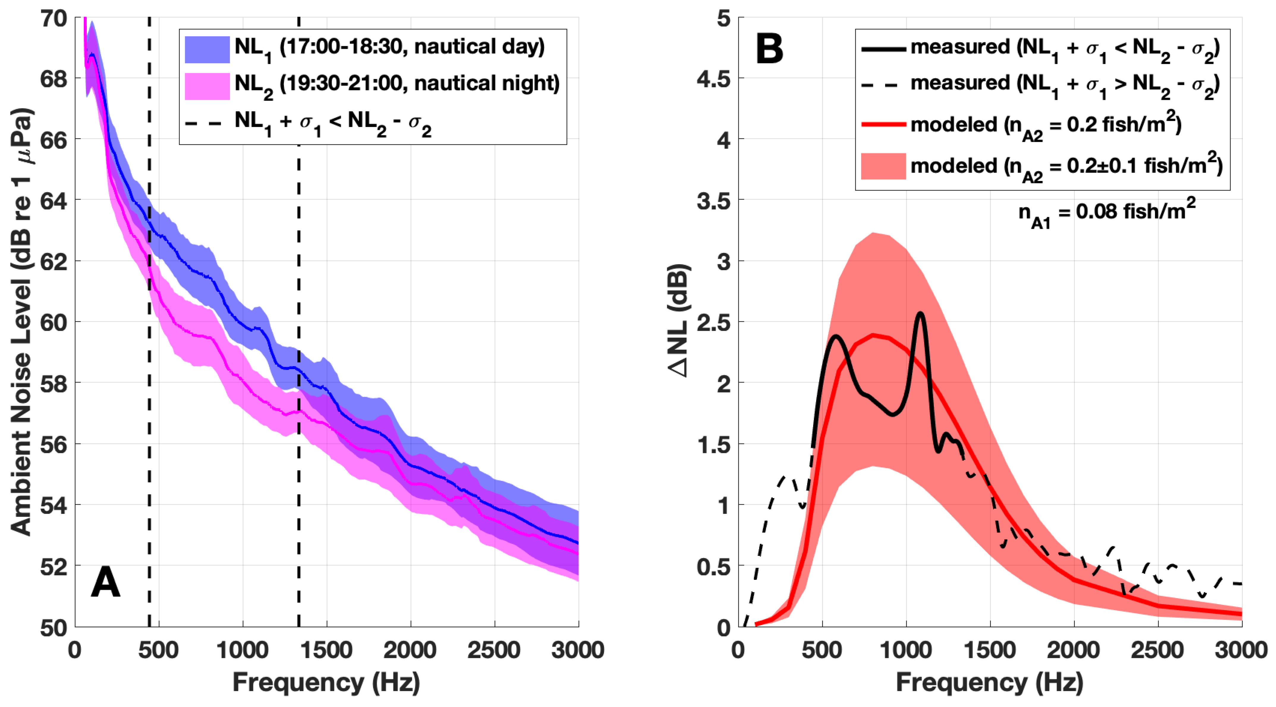
3.1. Ambient Noise Reductions from Fish-Attenuation

Reductions in the ambient noise level observed after nautical sunset are found to be consistent with the predicted reductions in ambient noise due to attenuation from fish (Figure 7). The decrease in ambient noise due to the formation of herring groups at nautical sunset on 20 February 2014 is predicted using Equation (13). The average areal density after nautical sunset ( n A 1 ) is determined to be 0.08 fish/m2 by taking the average of OAWRS areal density measurements between 17:00 and 18:30 (Figure 5D).
The average areal density after nautical sunset ( n A 2 ) is determined to be 0.2 fish/m2 by taking the average of OAWRS measurements of areal density between 19:30 and 21:00 (Figure 5D). The modeled coefficient for environmental attenuation excluding fish ϵ is determined by maximizing the following likelihood function:
( ϵ ) = i = 1 N f ( N L m o d e l ( ϵ , f i ) Δ N L ( f i ) ) σ Δ N L ( f i ) 2
where Δ N L ( f i ) is the mean reduction in ambient noise at frequency f i , σ Δ N L ( f i ) is the standard deviation at frequency f i , N f is the number of frequencies where Δ N L is measured, and the coefficient for environmental attenuation excluding fish ϵ is assumed to be in units of λ 1 . The likelihood function is maximized at ϵ = 5 × 10 5 λ 1 , which is in the same order of magnitude as previous experimental measurements of environmental attenuation in waveguide environments [18].

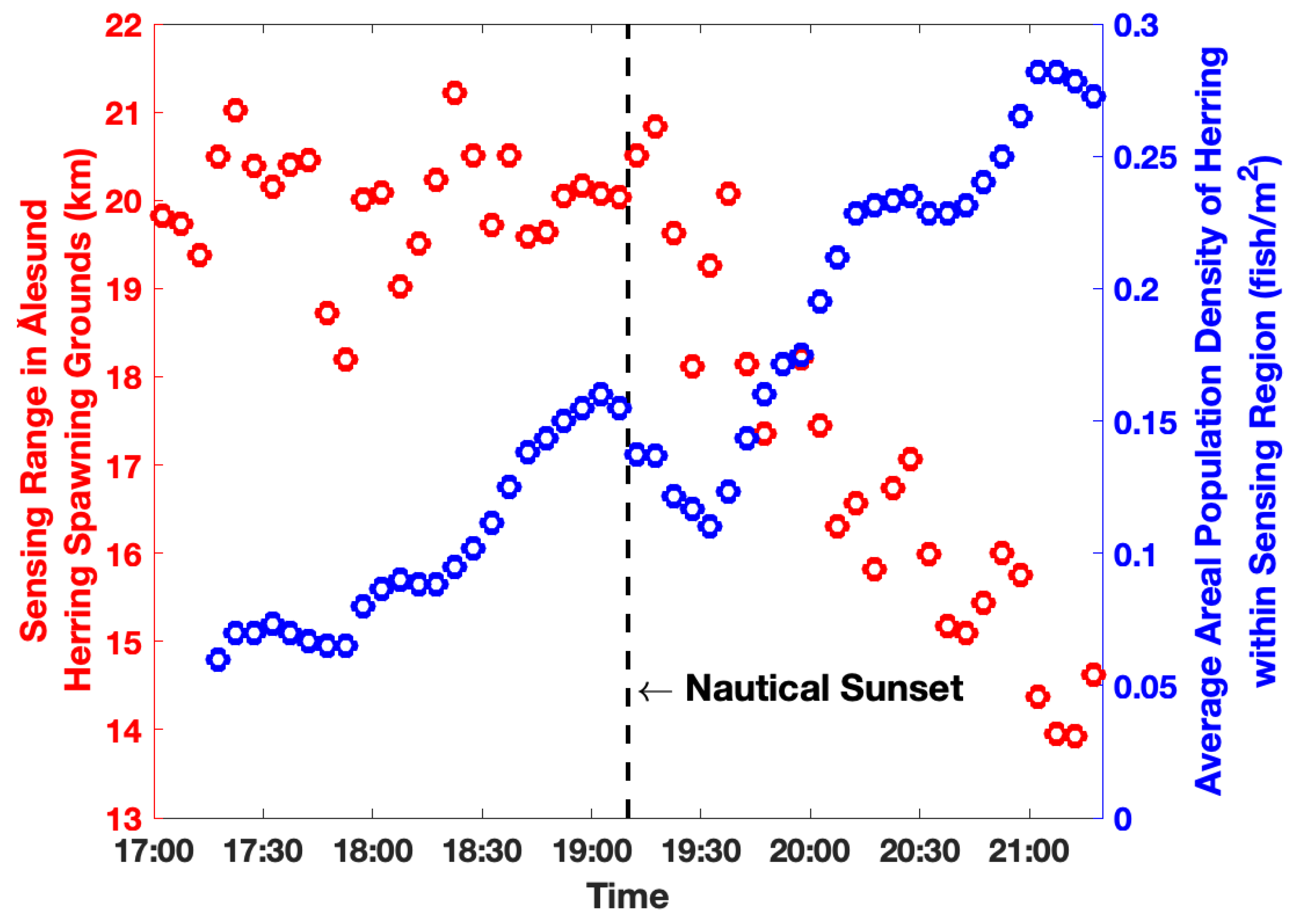
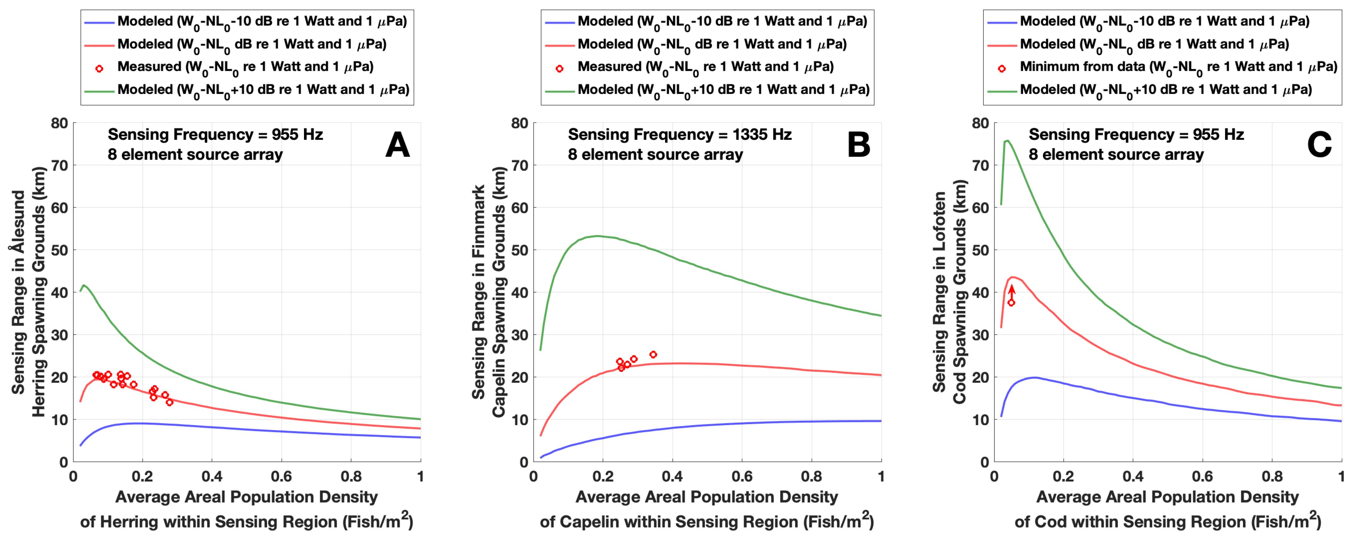
3.2. Sensing Range Reductions from Fish-Attenuation

The range-dependent decay in OAWRS transmissions due to attenuation from fish leads to significant reductions in the sensing range (Figure 8). Thirty minutes before nautical sunset, the average fish population density within the sensing region is below 0.1 fish/m2 and the sensing range remains approximately constant (20 km). In the two hours following nautical sunset, the fish population density increases to nearly 0.3 fish/m2, corresponding with reductions in the sensing range of 20%.
Measured reductions in sensing range are found to be theoretically predictable from waveguide scattering theory and observed population densities. Sensing range predictions depend on the average density of fish within the sensing region as well as the source power of the sensing system and ambient noise level (Section 2.4). The sensing range is predicted for both Ålesund herring and Finnmark capelin, and the predictions are in agreement with OAWRS measurements in both environments (Figure 9). The sensing range predictions for Lofoten cod exceed the maximum possible range that could be recorded in the 50 s recording window that was used in this region (Figure 9C). The formulation introduced here can be used to predict the performance of active sensing systems using historical surveys of fish population density in the relevant region, as well as fluctuations in the sensing range using known diel and annual variations in population density.

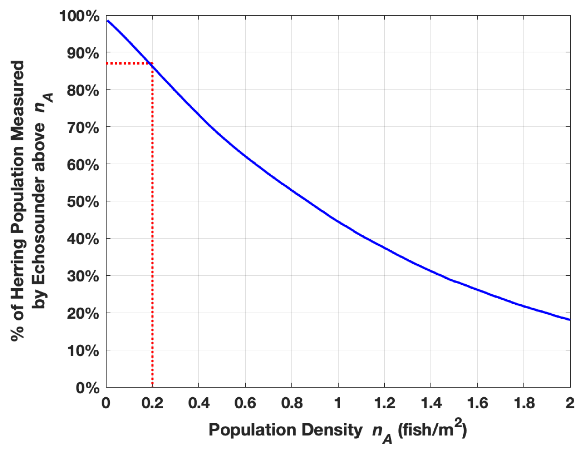
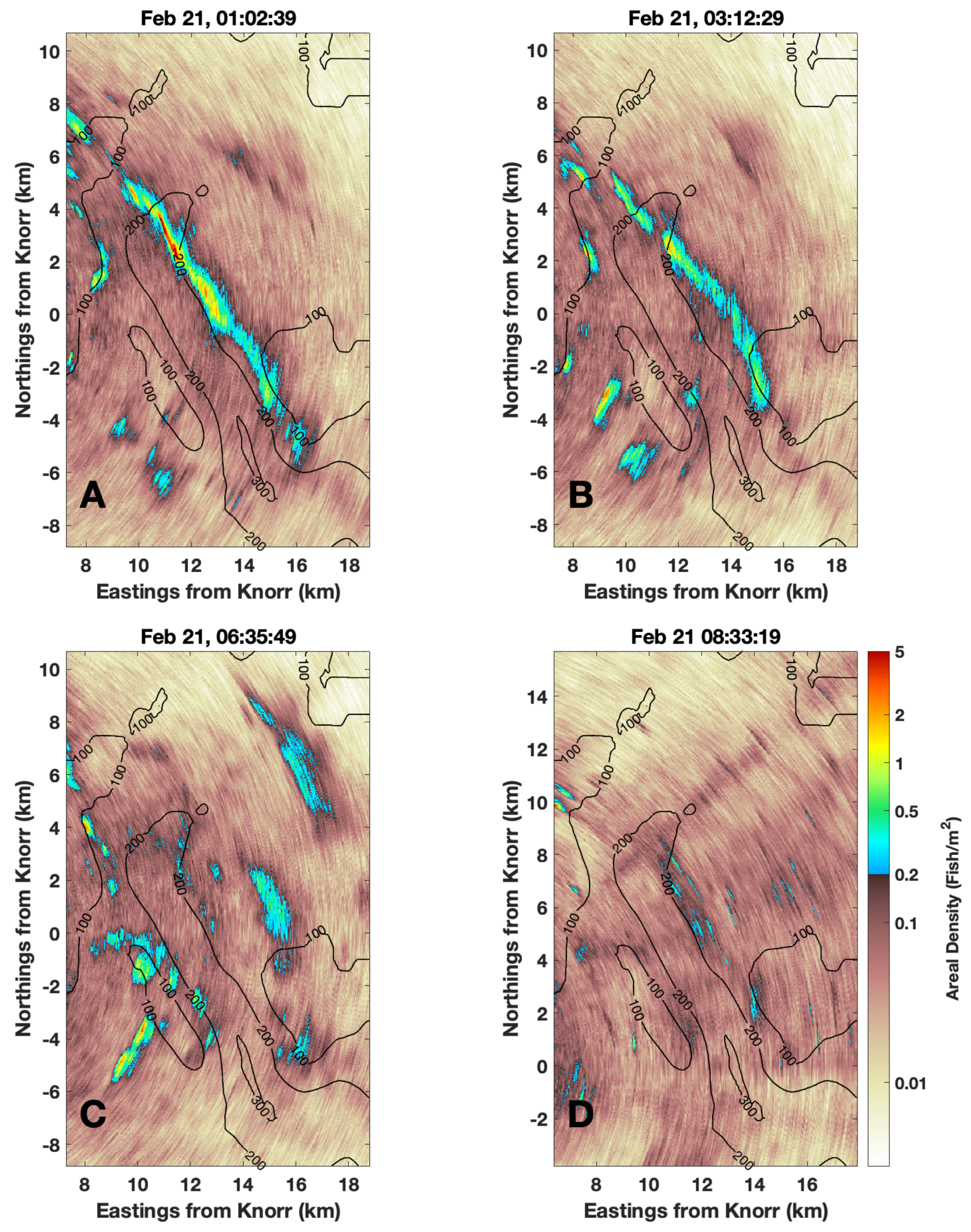
3.3. Spatial Undersampling in Echosounder Surveys

Spatial inhomogeneities in wide-area herring distributions seen synoptically in OAWRS imagery can be spatially undersampled in typical echosounder surveys, which can result in significant overestimation or underestimation of the fish population in the survey region. Equivalent echosounder estimates of herring population density, for example, are made by sampling 2014 spatially continuous OAWRS wide-area population density data (Figure 3, Figure 6 and Figure 10) with the sparse line-transects of a 2001 herring survey in the same region [20]. The measured population size within the survey box for each OAWRS image shown in Figure 10 is shown in Figure 11.
The total population estimate from line-transect sampling is then calculated by multiplying the average population density along the transect with a specified survey area (Figure 12A). Resulting population estimates in this area range from 0.5 to 2.5 times the population found using the entire OAWRS population density data for the region (Figure 12B). Wide-area spatial population density maps made with OAWRS can be used in conjunction with conventional line-transect survey methods to provide better estimates of herring population and spatial distribution.

4. Discussion

It is experimentally shown that Ocean Acoustic Waveguide Remote Sensing (OAWRS) can be used to instantaneously measure wide-area fish population density, even in environments where sensing is affected by attenuation from fish. OAWRS imagery of Norwegian spring-spawning herring is corrected for attenuation in a manner consistent with waveguide scattering theory in order to produce population density maps over more than one thousand square kilometers during dense shoaling activity. We found that attenuation from dense herring groups forming after nautical sunset on February 20 resulted in reductions in sensing range of roughly 20%.
It is also shown that attenuation from fish groups forming at nautical sunset can result in ambient noise reductions. In future experiments, it may be possible to make crude inferences about diel changes in fish population density from fluctuations in ambient noise. It has been previously shown that attenuation from Norwegian herring can be significant at the sensing frequencies and typical shoaling densities in this experiment, and attenuation can be significantly reduced in this environment by choosing sensing frequencies above or below the swimbladder resonance of the herring (>2 kHz or <500 Hz) [12]. Such attenuation requires exceptionally high fish population densities over significant portions of the water column and extended ranges and, thus, was not observed previously in OAWRS sensing of swimbladder-bearing fish including Mid-Atlantic Bight herring [5], Gulf of Maine herring [6], and Lofoten cod [10].

5. Conclusions

Ocean Acoustic Waveguide Remote Sensing (OAWRS) is used to instantaneously monitor spawning Norwegian herring population densities over wide areas, spanning more than one thousand square kilometers, in the Nordic Seas near the Ålesund trench where herring are known to spawn. Larger spawning shoals often spanning a few kilometers are instantaneously imaged in their entirety. Reductions of roughly 20% in sensing range after sunset have been found due to the corresponding formation of larger and denser herring shoals after sunset for OAWRS transmissions near swimbladder resonance.
This attenuation is corrected for in a manner consistent with waveguide scattering theory, leading to instantaneous wide-area OAWRS population density maps up to the sensing range of ambient noise limitation. Sensing range reductions due to attenuation from fish are shown to be theoretically predictable from waveguide scattering theory and observed population densities. Such sensing range reductions may also limit the ability of vocalizing marine mammals to echolocate in regions with dense fish shoals [21,22].
Spatial-temporal inhomogeneities in wide-area herring distributions observed by OAWRS indicate that large errors are expected in the population density estimates made from sparse line-transect surveys through this region during spawning. This is due to the significant temporal and spatial aliasing of the non-homogeneous herring population density distributions observed by OAWRS. The population density maps provided by OAWRS can then be used in conjunction with conventional line-transect survey methods to efficiently provide more accurate estimates of herring populations and temporal-spatial distributions.

Author Contributions

Conceptualization, N.C.M. and O.R.G.; formal analysis, D.D. and N.C.M.; funding acquisition, N.C.M. and O.R.G.; conducting experiment at sea, N.C.M. and O.R.G.; methodology, D.D. and N.C.M.; project administration, N.C.M. and O.R.G.; resources, N.C.M. and O.R.G.; software, D.D. and N.C.M.; supervision, N.C.M.; validation, D.D. and N.C.M.; visualization, D.D. and N.C.M.; writing—original draft, D.D. and N.C.M.; writing—review & editing, N.C.M. and D.D. All authors have read and agreed to the published version of the manuscript.

Funding

This research was funded by Office of Naval Research grant number N00014-17-1-2197.

Conflicts of Interest

The authors declare no conflict of interest.

Appendix A. Measurement of Scattering Strength

Data presented here is from an OAWRS experiment conducted in 2014 to survey fish populations in the Nordic Seas via continuous monitoring with instantaneous wide-area sensing. Roughly 10,000 active transmissions were recorded at frequencies between 850 and 1600 Hz. The experiment covered multiple species in four regions in the Nordic Seas: herring in the Ålesund region were studied from 18–21 February, cod in the Lofoten region were studied on 23 February and 5–7 March, capelin in the Finnmark region were studied from 26–28 February and 1–3 March, and capelin in the Tromso region were studied from 28 February through 1 March. OAWRS data was produced from active transmissions of 1 s duration linear-frequency-modulated waveforms from a vertical source array attached to the research vessel (Figure A1). Scattered returns from environmental features are received by a horizontal line array towed by the same research vessel with multiple nested sub-apertures. Three linear apertures of the receiver array, i.e., the low-frequency (LF) aperture, the mid-frequency (MF), and the high frequency (HF) aperture, consist of 64 equally spaced hydrophones with respective inter-element spacing of 1.5 m, 0.75 m, and 0.375 m. Images are generated by beamforming, matched filtering, and charting scattered returns, using nonuniformly-spaced combinations of the LF, MF, and HF apertures, as described in [16].
In cases where there is not significant attenuation from fish, scattering strength S S can be calculated [4,5,6,7] from
S S = 10 log 10 Ψ Ψ r e f 2 S L T L A
where Ψ is the scattered field, Ψ r e f = 1 μ Pa is the reference acoustic pressure in water, S L is the source level, T L A is the depth-averaged two-way transmission loss to individual scatterers integrated over OAWRS imagining resolution, given [6] by
T L A = 10 log 10 A R ( ρ C ) 1 H z 0 H / 2 z 0 + H / 2 χ r , r 0 , r T d z T d ρ T 2 / r r e f 2
where z 0 is the center depth of the fish layer, H is the vertical thickness of the fish layer, and χ r , r 0 , r T is the magnitude squared of the two-way Green function from source r 0 to target r T to receiver r , given by
χ r , r 0 , r T = ( 4 π ) 4 G r | r T ; f , c ( r w ) , d ( r w ) 2 G r T | r 0 ; f , c ( r w ) , d ( r w ) 2 | r T
where G r | r T ; f , c ( r w ) , d ( r w ) is the Green function between the target location r T = ( ρ T , z T ) and the receiver location r , ρ T = ( x T , y T ) is the horizontal target location, G ( r T | r 0 ; f , c ( r w ) , d ( r w ) ) is the Green function between the source location r 0 = ( ρ S , z S ) and the target location r T , c ( r w ) and d ( r w ) are the sound speed and density of any point r w in the propagation path, respectively. While χ r , r 0 , r T includes transmission losses due to spreading and seafloor attenuation, it does not include losses due to attenuation from fish. A parabolic equation model [23] is used to calculate the Green functions in a range-dependent environment. The conditional expectation over the sound speed is determined by averaging five Monte-Carlo realizations, where the Green functions are calculated along the propagation path in range and depth for each realization. Each Monte-Carlo realization employs sound-speed profiles measured during the 2014 OAWRS experiment (Appendix F of [12]) every 500 m along the propagation path [18].
In cases where there is significant attenuation from fish (Figure 4), scattering strength uncorrected for attenuation from fish ( S S ˜ ) can be calculated from
S S ˜ S S Δ S P L 2 w a y = 10 log 10 Ψ Ψ r e f 2 S L T L A
where Δ S P L 2 w a y is the decrease in sound pressure level due to two-way attenuation from fish. Measurements of fish-attenuated scattering strength can be corrected using the method described in Section 2.2.
Figure A1. OAWRS system used for herring measurements during the Nordic Seas 2014 Experiment [10]. The system is effectively monostatic with source and receiver arrays were towed from the same research vessel (RV Knorr). The OAWRS source was developed under the National Science Foundation and Sloan Foundation MRI program for wide-area sensing of marine life, and the ONR Five Octave Research Array (FORA) was used as the OAWRS receiver.
Remotesensing 13 04546 g0a1

Appendix B. Calibration of Target Strength

Scattering strength is converted to areal population density by calibration with local in situ measurements of areal population density obtained from echosounder measurements. This calibration is performed using OAWRS images of the large, elongated herring shoal observed on February 21 (Figure A2A) with a nearly concurrent echosounder transect (Figure A2B). Areal density n A at range r along the transect is calculated according to Equation (A32). Target strength measured by OAWRS at frequency f i and range r along the transect is calculated according to:
T S d a t a ( f i , r ) = 10 log 10 ( 10 ( S S d a t a ( f i , r ) 10 log 10 ( n A ( r ) ) ) / 10 )
where S S d a t a ( f i , r ) is the scattering strength measured by OAWRS at range r along the transect and sensing frequency f i (Appendix A). Neutral buoyancy depth z n b is then determined by modeling target strength T S m o d e l ( z n b , f i ) according to Appendix E assuming the measured distribution of herring depths (Figure A2C) and maximizing the following likelihood function:
( z n b ) = i = 1 N f ( T S m o d e l ( z n b , f i ) T S d a t a ( f i ) ) σ T S ( f i ) 2
where T S d a t a ( f i ) is the mean target strength measured along the transect at frequency f i , σ T S ( f i ) is the standard deviation at frequency f i , and N f is the number of frequencies. The likelihood function is maximized by searching for across possible neutral buoyancy depths from sea surface to seafloor, and calibrated neutral buoyancy depth is determined to be z n b = 3 m below the sea surface (Figure A2D).
OAWRS scattering strength maps are then converted to areal population density maps according to:
10 log 10 ( n A ( ρ , θ ) = S S ( ρ , θ ) + T S ( z n b , f )
where n A is the areal population density at range ρ and azimuth θ , S S is the OAWRS scattering strength, f = 955 is the frequency of the OAWRS transmissions shown here, and z n b is the calibrated neutral buoyancy depth.
Figure A2. The target strength of herring in Ålesund is determined by calibrating OAWRS scattering strength measurements of a large, elongated herring shoal observed on 21 February with nearly concurrent echosounder transects. The OAWRS scattering strength map from 21 February 2014 at 3:26:39 at sensing frequency 955 Hz is shown in (A) with the echosounder transect from 2:52:00–2:58:00 overlain in white. Echosounder data is shown in (B), where vertical black dotted lines denote the transect studied here. The average areal population density along the echosounder transect is shown in (C), and average volume density of herring with respect to depth along this transect is shown in (D). The target strength of herring in this shoal is modeled assuming the depth distribution shown in (D), and neutral buoyancy depth is determined to be 3 m by performing a least-squares fit between measured and modeled target strength (E).
Remotesensing 13 04546 g0a2

Appendix C. Measuring Sensing Range

Sensing range ρ s e n s is measured as the maximum range ρ at which the azimuthally intensity-averaged sound-pressure level S P L A is greater than the attenuated ambient noise over the frequency band of the signal by more than the detection threshold D T :
ρ s e n s = max [ ρ | S P L A ( ρ ) > N L Δ N L + D T ]
where N L is the ambient noise level and Δ N L is the reduction in ambient noise due to attenuation from fish over the frequency band of the signal. Here, the detection threshold D T is set at 5.6 dB, which is the standard deviation of an acoustic measurement after saturated multipath propagation when the time-bandwidth product is one [15,24]. The azimuthally intensity-averaged sound-pressure level S P L A ( ρ ) is calculated by averaging the intensity of the beamformed scattered field across azimuthal angle θ over multiple transmissions within the relevant time frame:
S P L A ( ρ ) 10 log 10 Ψ ( ρ ) Ψ r e f 2 = 10 log 10 1 N k = 1 N 1 θ m a x θ m i n θ m i n θ m a x Ψ ( k ) ( ρ , θ ) Ψ r e f 2 d θ
where Ψ ( k ) ( ρ , θ ) is the beamformed scattered field from transmission k at range ρ and azimuthal angle θ , N is the number of transmissions within the time frame analyzed, Ψ r e f = 1 μ Pa is the reference pressure for underwater sound, Ψ ( ρ ) 2 is the magnitude squared of the beamformed scattered field averaged over θ and k, and the limits of integration θ m i n and θ m a x are chosen to exclude beams within 25° of endfire.
Attenuated ambient noise over the frequency band of the signal ( N L Δ N L ) is measured from the average acoustic intensity above a minimum range ρ m i n :
N L Δ N L = 10 log 10 1 ρ m a x ρ m i n ρ m i n ρ m a x Ψ ( ρ ) Ψ r e f 2 d ρ
where ρ m a x = 33 km is the maximum recorded range, determined by the recording time for each OAWRS transmission, and ρ m i n is the range after which we can safely say that ambient noise dominates the received sound pressure level for each OAWRS transmission. ρ m i n is chosen so that the recorded sound pressure level between ρ m i n and ρ m a x does not significantly change with range, indicating that the measured sound pressure level is dominated by ambient noise. This is quantified by expressing ρ m i n as:
ρ m i n = min ρ m i n | 1 N k = 1 N | β ( k ) ( ρ m i n ) | < β t h r e s h o l d
where β ( k ) ( ρ m i n ) is the slope of the linear regression of sound pressure level with respect to range for transmission k between ρ m i n and ρ m a x , given by:
β ( k ) ( ρ m i n ) = ρ m i n ρ m a x ( S P L A ( k ) ( ρ ) ρ m i n ρ m a x S P L A ( k ) ( ρ ) d ρ ) ( ρ 1 2 ( ρ m a x ρ m i n ) d ρ ρ m i n ρ m a x ( ρ 1 2 ( ρ m a x ρ m i n ) ) d ρ
where S P L A ( k ) ( ρ ) is the range-dependent sound pressure level for a single transmission k, and β t h r e s h o l d is the maximum slope at which we determine the sound pressure level to be sufficiently flat with respect to range. Setting the slope threshold at β t h r e s h o l d = 0.01 dB/km, ρ m i n is calculated as 29.5 km. Visual inspection of Figure A3C,D confirms that measured sound pressure level flattens with respect to range above 29.5 km.
Combining Equations (A8) and (A10) yields the following formulation for measuring sensing range:
ρ s e n s = max ρ | S P L A ( ρ ) > 10 log 10 1 ρ m a x ρ m i n ρ m i n ρ m a x Ψ ( ρ ) Ψ r e f 2 d ρ + D T
Sensing range at azimuthal angle θ for OAWRS transmission k can be similarly defined as:
ρ s e n s ( k ) ( θ ) = max ρ | S P L A ( k ) ( ρ , θ ) > 10 log 10 1 ρ m a x ρ m i n ρ m i n ρ m a x Ψ ( k ) ( ρ ) Ψ r e f 2 d ρ + D T
Example measurements of sensing range are shown in Figure A3, where a 20% reduction is observed after nautical sunset.
Figure A3. Reductions in signal intensity and ambient noise caused by attenuation from herring groups resulted in a 20% reduction in the sensing range after nautical sunset. “Sensing range” is defined here as the range at which scattered returns from the environment can be observed above ambient noise. OAWRS maps of normalized pressure level are generated by averaging 12 instantaneous OAWRS images at 955 Hz at 17:00–17:10 (A) and 21:00–21:00 (B). The mean sensing range over each hour-long interval is calculated by averaging each sound pressure level map across all azimuthal angles, excluding angles within 25° of endfire (C,D). Sensing range (red dots in (C,D)) is measured as the range where sound pressure level (blue lines in (C,D)) falls within the detection threshold D T = 5.6 dB of the ambient noise. Over the course of the four hours shown here, sensing range reduces by 20%. Light blue patches in (C,D) denote the standard deviation of normalized pressure level. The pressure levels shown here are normalized by the ambient noise level measured between 17:00 and 17:10 (A,B).
Remotesensing 13 04546 g0a3

Appendix D. Modeling Two-Way Attenuation in a Waveguide Environment

The decrease in sound pressure level due to attenuation from fish during two-way propagation can be expressed [12] as
Δ S P L 2 w a y = 10 log 10 Ψ i , 2 w a y r | r 0 2 10 log 10 Ψ T , 2 w a y r | r 0 2
where Ψ i , 2 w a y r | r 0 2 is the intensity of the two-way scattered field without attenuation from fish and Ψ T , 2 w a y r | r 0 2 is the total mean intensity of the two-way scattered field with attenuation from fish. For a distribution of fish with scatter function S and volume number density n V , the intensity of the scattered field without attenuation at resolution footprint A R ( ρ C ) can be written [12] as
Ψ i , 2 w a y r | r 0 2 = A R ( ρ C ) z Ψ i r t | r 0 2 S ( z t ) k 2 n V ( r t ) Ψ i r | r t 2 d z t d ρ t 2
where Ψ i r t | r 0 is the incident field from source r 0 = ( ρ 0 , z 0 ) to target r t = ( ρ t , z t ) and Ψ i r | r t is the field scattered from target r t = ( ρ t , z t ) to receiver r = ( ρ , z ) , defined according to
Ψ i r | r 0 = n Ψ i ( n ) r | r 0
where Ψ i ( n ) r | r 0 is the contribution to the field by mode n, S is the scatter function of an individual fish with respect to depth z as defined in Equation (A27), and with the approximation that it is uniform in range, the depth-dependent volumetric population density n V is
n V ( r t ) = n A p ( z t )
where n A is the constant areal population density and p ( z ) is the probability distribution function of herring depth, which is determined from echosounder measurements during the experiment and explicitly defined in Appendix F. The mean intensity of the scattered field including attenuation can be written as
Ψ T , 2 w a y r | r 0 2 = A R ( ρ C ) z Ψ T r t | r 0 2 S ( z t ) k 2 n V ( r t ) Ψ T r | r t 2 d z t d ρ t 2
where Ψ T r t | r 0 2 is the total mean intensity from source r 0 to target r t and Ψ T r | r t 2 is the total mean intensity from target r t to receiver r , defined according to
Ψ T r | r 0 2 = Ψ T r | r 0 2 + Var Ψ T r | r 0
where Ψ T r | r 0 is the total mean forward field in an acoustic waveguide with scatterers and Var Ψ T r | r 0 is the variance of the forward field. The total mean forward field with scatterers can be expressed as
Ψ T r | r 0 = n Ψ i ( n ) r | r 0 e i 0 ρ ν n ( ρ s ) d ρ s
where each dispersion and attenuation coefficient ν n describes the change in the horizontal wavenumber of mode n as it propagates through the scatterers. Dispersion and attenuation coefficients depend on the horizontal wavenumber ξ n , the shape of the corresponding mode u n , the volume density of the scatterers n V and the scatter function of an individual scatterer S. A general formulation for ν n can be found in Equation (60a) of Reference [13]. Since long-range ocean sensing systems typically operate at low frequencies where the acoustic wavelength is larger than the dimensions of a fish, individual fish will be compact scatterers and the dispersion and attenuation coefficients for fish shoals can be obtained from Equations (19) and (60a) of Reference [13]:
ν n ( ρ ) = 0 2 π k 1 ξ n 1 d ( z t ) ( u n ( z t ) ) 2 s ( ρ , z t ) d z t
where s ( ρ , z ) is the expected scatter function density of the scatterers. Since the spacing between individual fish is larger than the acoustic wavelength, the fish are incoherent scatterers and the expected scatter function density of a group of fish can be expressed as s ( ρ , z ) = n V ( ρ , z ) S ( z ) , where n V is defined according to Equation (A18).
The variance of the forward field can be expressed as
Var Ψ T r | r 0 = n 2 π d 2 ( z 0 ) 1 ξ n ρ u n ( z 0 ) 2 u n ( z ) 2 e 2 ξ n ρ + 0 ρ ν n ( ρ s ) d ρ s e 0 ρ μ n ( ρ s ) d ρ s 1
where μ n ( ρ ) is the exponential coefficient of modal field variance. A general formulation for μ n can be found in Equation (94a) of Reference [13]. Since the scatter function of an individual fish is omnidirectional in long-range ocean sensing applications, the exponential coefficient of modal field variance for fish shoals can be obtained from Equations (19), (72) and (94a) of Reference [13]:
μ n ( ρ s ) = m ρ 2 π ξ m ρ s ( ρ ρ s ) 1 ξ m 0 4 π 2 k 2 d 2 ( z t ) u n ( z t ) 2 u m ( z t ) 2 V c ( z t ) Var ( s ( ρ , z t ) ) d z t
where the scatter function coherence volume V c quantifies the spatial scale over which the scatter functions of two fish are correlated. The variance of the scatter function density for incoherent scatterers can be obtained from Equation (A23) of Reference [13]:
Var ( s ) = 1 V c n V Var S
The exponential coefficient of model field variance μ n (Equation (A24)) is independent of the coherence volume V c since the scatterers are incoherent.

Appendix E. Modeling the Target Strength of an Individual Fish

The target strength of an individual fish in a shoal is determined [6] by
T S = 10 log 10 1 H z l S k 2 p ( z ) g ( l ) d l d z
where k is the wavenumber, l is the fork length of an individual fish as measured from trawl samples, g ( l ) is the Gaussian probability density function of the fork length, z is the fish depth, p ( z ) is the probability density function of fish depth as determined by echosounder measurements (Figure A6), and S is the far-field scatter function of an individual fish, given [25] by:
S ( z , z n b , l , f ) = f 0 2 ( z , z n b , l ) f 2 1 k a ¯ ( z , z n b , l ) f 0 2 ( z , z n b , l ) f 2 1 2 + δ 2 ( z , z n b , l , f ) + i δ ( z , z n b , l , f ) k a ¯ ( z , z n b , l ) f 0 2 ( z , z n b , l ) f 2 1 2 + δ 2 ( z , z n b , l , f )
where k is the wavenumber, f is the sensing frequency, f 0 ( z , z n b , l ) is the resonance frequency of swimbladder, a ¯ ( z , z n b , l ) is the equivalent swimbladder radius and δ ( z , z n b , l , f ) is a dimensionless damping coefficient. The mean fork length l for herring is 34 m and the neutral buoyancy depth is 3 m (Appendix B). The equivalent swimbladder radius is determined [26] by
a ¯ ( z , z n b , l ) = 3 4 π c n b m f l e s h ( l ) ρ f l e s h 1 + z n b / 10 1 + z / 10 1 / 3
assuming that the swimbladder volume varies with pressure according to Boyle’s law, where c n b is the ratio of the swimbladder volume at neutral buoyancy to the volume of the fish flesh V f l e s h = m f l e s h ( l ) / ρ f l e s h . m f l e s h ( l ) is the mass of a single fish empirically determined by the fork length l [7] and ρ f l e s h is the density of the fish flesh. The resonance frequency of the swimbladder is determined by
f 0 ( z , z n b , l ) = κ ( ϵ ( z , z n b , l ) ) 2 π r ( z , z n b ) 3 γ P a t m ( 1 + z / 10 ) ρ f l e s h
where γ = 1.4 is the ratio of the specific heats of air and P a t m = 1.013 Pa is the atmospheric pressure. The correction term κ ( ϵ ( z , z n b , l ) ) is a function of ϵ ( z , z n b , l ) , the swimbladder’s eccentricity. The correction term κ ( ϵ ( z , z n b , l ) ) for a prolate spheroidal swimbladder is given [27] by:
κ ( ϵ ( z , z n b , l ) ) = 2 ( 1 ϵ 2 ( z , z n b , l ) ) 1 / 4 ϵ 1 / 3 ( z , z n b , l ) ln 1 + 1 + ϵ 2 ( z , z n b , l ) 1 1 ϵ 2 ( z , z n b , l ) 1 / 2
where ϵ ( z , z n b , l ) is the ratio of the minor to major axis of a prolate spherical swimbladder given by ϵ ( z , z n b , l ) = c s b l a ¯ ( z , z n b , l ) 3 / 2 and c s b is the ratio of the major axis of the swimbladder to the fish fork length l [7].
The dimensionless damping coefficient δ ( z , z n b , l , f ) in Equation (A27) is obtained from the sum of radiation damping δ r a d and viscous damping δ v i s :
δ ( z , z n b , l , f ) = δ r a d + δ v i s = 2 π f a ¯ ( z , z n b , l ) c + ξ f π a ¯ 2 ( z , z n b , l ) f ρ f
where f is the frequency, c is the sound speed, ξ f is the viscosity of the fish flesh and ρ f is the density of fish flesh [8].

Appendix F. Synoptic Echosounder Measurements of Herring Areal Density and Depth Distribution

Synoptic echosounder measurements of Ålesund herring population density collected during the 2014 OAWRS experiment (Figure A5) are consistent with estimates of herring population shown in Figure 5. Shoal volume density (fish/m3) is measured from echogram data according [7] to
n V = 1 σ b s s v
where s v is the volume backscattering coefficient (m−1) and σ b s = 10 T S C F F S / 10 is the fish backscattering cross section of an individual fish at at the echosounder sensing frequency (38 kHz) in units of m2, where T S C F F S is the target strength at this frequency, given [28] by
T S C F F S = 20 log 10 L T L 2.3 log 10 ( 1 + z / 10 ) 65.4
where L T L is the length of an individual herring (cm), and z is the water depth (m). Shoal areal density (fish/m2) is given by
n A = z 1 z 2 n V d z
where z 1 and z 2 delimit the depth bounds of the fish aggregations.
The probability density function of herring depth p ( z ) is measured by aggregating echosounder measurements of herring in Ålesund waters according to:
p ( z ) = ρ n V , C F F S ( ρ , z ) d ρ z ρ n V , C F F S ( ρ , z ) d ρ d z
where n V , C F F S ( ρ , z ) is the volumetric population density of herring at horizontal position ρ and depth z measured by echosounders between 17:00 and 21:00 on 20 February, where p ( z ) appears in Figure A6.
Figure A4. Synoptic echosounder measurements of Ålesund herring shoals are consistent with OAWRS population density measurements before nautical sunset. In (A), bathymetric contours are shown in black, the path of the research vessel towing the OAWRS system (RV Knorr) between 17:00 and 18:30 on 20 February 2014 is overlain in blue, and the path of the research vessel from which echosounder measurements were recorded during this time is overlain in magenta. Echosounder measurements of volumetric population density are shown in (B), and measurements of areal population density are shown in (C). Sparse herring groups are observed with population densities on the order of 0.3 fish/m2, which is consistent with OAWRS population density measurements during this time (Figure 3).
Remotesensing 13 04546 g0a4
Figure A5. Synoptic echosounder measurements of Ålesund herring shoals are consistent with OAWRS population density measurements after nautical sunset. In (A), bathymetric contours are shown in black, the path of the research vessel towing the OAWRS system (RV Knorr) between 19:30–21:00 on 20 February 2014 is overlain in blue, and the path of the research vessel from which echosounder measurements were recorded during this time is overlain in magenta. Echosounder measurements of volumetric population density are shown in (B), and measurements of areal population density are shown in (C). Several dense herring groups are observed with population densities on the order of 5 fish/m2, which is consistent with OAWRS population density measurements during this time (Figure 6).
Remotesensing 13 04546 g0a5
Figure A6. Probability density function of herring depth p ( z ) inverted from echosounder measurements on 20 February 2014 between 17:00 and 21:00 in Ålesund spawning grounds (Equation (A35)).
Remotesensing 13 04546 g0a6

Appendix G. Measurements of Herring Population from OAWRS Population Density Maps

Herring population within OAWRS survey regions is calculated by integrating OAWRS measurements of population density over regions where the population density is greater than 0.2 fish/m2, which is the critical population density at which large herring shoals were found to form [4,5]. It is found that selecting regions above this threshold is an effective way to include discrete herring shoals in population measurements without including measurements contaminated by background seafloor scattering (Figure A7). It is found that 87% of the herring population measured by echosounders during this experiment was above the 0.2 fish/m2 threshold (Figure A8).
Figure A7. Echosounder measurements confirm that the majority of herring contained in the discrete shoals observed by OAWRS are in regions where the population density is greater than the critical population density 0.2 fish/m2 [4,5]. An OAWRS population density map from 21 February, 3:26:39 is shown in (A), where the path of an echosounder is overlain in white and the corresponding echosounder data from 2:48–3:40 are shown in (B). The green dot in (A) and the green line in (B) correspond to the echosounder position for the OAWRS image shown in (A). Black dotted lines in (B) designate regions α , β , and γ , where both systems co-register dense fish groups (A). The areal population density measured by the echosounder along this transect is shown in (C), where red data denotes regions where the OAWRS population density is greater than 0.2 fish/m2 and black data denotes regions where the OAWRS population density is less than 0.2 fish/m2. It is found that selecting regions above the 0.2 fish/m2 threshold is an effective way to segment discrete herring shoals (red data in (C)) without including measurements potentially affected by scintillation and contamination from background seafloor scattering (black data in (C)). By contrast, a significant portion of OAWRS data above 0.05 fish/m2 falls outside the dense, discrete shoal (D).
Remotesensing 13 04546 g0a7
Figure A8. The percentage of the herring population measured by echosounders between 17 February, 23:30 and 21 February, 21:00 above the population density threshold n A is shown here. 87% of the herring population is found to be above the critical population density 0.2 fish/m2 (red dotted line).
Remotesensing 13 04546 g0a8

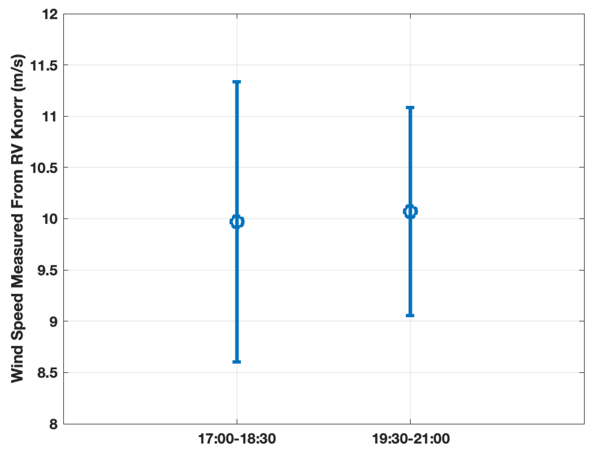
Appendix H. Measured Wind Speed Variations

Figure A9. Wind speed measurements recorded by the research vessel towing the OAWRS system (RV Knorr) are shown here from 20 February 2014 between 17:00–18:30 (before nautical sunset) and between 19:30–21:00 (after nautical sunset). There is no statistically significant difference between wind speed before and after sunset, indicating that reductions in ambient noise after sunset are not caused by changes in wind speed.
Remotesensing 13 04546 g0a9
Wind speed measurements recorded by the research vessel towing the OAWRS system (RV Knorr) before and after nautical sunset on 20 February 2014 are shown in Figure A9. There is no statistically significant difference between wind speed before and after sunset, which demonstrates that reductions in ambient noise after sunset are not caused by changes in wind speed.

References

  1. Marine Stewardship Council. International Action Needed on Herring and Blue Whiting Stocks. 2020. Available online: https://www.msc.org/media-centre/news-opinion/news/2020/12/04/international-action-needed-on-herring-and-blue-whiting-stocks (accessed on 18 August 2021).
  2. Berdahl, A.; Westley, P.A.; Levin, S.A.; Couzin, I.D.; Quinn, T.P. A Collective Navigation Hypothesis for Homeward Migration in Anadromous Salmonids. Fish Fish. 2016, 17, 525–542. [Google Scholar] [CrossRef] [Green Version]
  3. Klemas, V. Fisheries Applications of Remote Sensing: An Overview. Fish. Res. 2013, 148, 124–136. [Google Scholar] [CrossRef]
  4. Makris, N.C.; Ratilal, P.; Jagannathan, S.; Gong, Z.; Andrews, M.; Bertsatos, I.; Godø, O.; Nero, R.; Jech, J.M. Critical population density triggers rapid formation of vast oceanic fish shoals. Science 2009, 323, 1734–1737. [Google Scholar] [CrossRef] [Green Version]
  5. Makris, N.C.; Ratilal, P.; Symonds, D.; Jagannathan, S.; Lee, S.; Nero, R. Fish population and behavior revealed by instantaneous continental shelf-scale imaging. Science 2006, 311, 660–663. [Google Scholar] [CrossRef]
  6. Jagannathan, S.; Bertsatos, I.; Symonds, D.; Chen, T.; Nia, H.; Jain, A.; Andrews, M.; Gong, Z.; Nero, R.; Ngor, L.; et al. Ocean Acoustics Waveguide Remote Sensing (OAWRS) of marine ecosystems. Mar. Ecol. Prog. Ser. 2009, 395, 137–160. [Google Scholar] [CrossRef]
  7. Gong, Z.; Andrews, M.; Jagannathan, S.; Patel, R.; Jech, J.M.; Makris, N.C.; Ratilal, P. Low-frequency target strength and abundance of shoaling Atlantic herring (Clupea harengus) in the Gulf of Maine during the Ocean Acoustic Waveguide Remote Sensing 2006 Experiment. J. Acoust. Soc. Am. 2010, 127, 104–123. [Google Scholar] [CrossRef]
  8. Andrews, M.; Gong, Z.; Ratilal, P. Effects of multiple scattering, attenuation, and dispersion in waveguide sensing of fish. J. Acoust. Soc. Am. 2011, 130, 1253–1271. [Google Scholar] [CrossRef]
  9. Yi, D.H.; Gong, Z.; Jech, J.M.; Ratilal, P.; Makris, N.C. Instantaneous 3D continental-shelf scale imaging of oceanic fish by multi-spectral resonance sensing reveals group behavior during spawning migration. Remote Sens. 2018, 10, 108. [Google Scholar] [CrossRef] [Green Version]
  10. Makris, N.C.; Godø, O.R.; Yi, D.H.; Macauley, G.J.; Jain, A.D.; Cho, B.; Gong, Z.; Jech, J.M.; Ratilal, P. Instantaneous areal population density estimation of entire Atlantic cod and herring spawning groups and group size distribution relative to total spawning population. Fish Fish. 2018, 20, 201–213. [Google Scholar] [CrossRef] [Green Version]
  11. Wang, D.; Garcia, H.; Tran, D.D.; Jain, A.D.; Yi, D.H.; Gong, Z.; Jech, J.M.; Godø, O.R.; Makris, N.C.; Ratilal, P. Vast assembly of vocal marine mammals from diverse species on fish spawning ground. Nature 2016, 531, 366–369. [Google Scholar] [CrossRef] [PubMed]
  12. Duane, D.; Cho, B.; Jain, A.D.; Godø, O.R.; Makris, N.C. The Effect of Attenuation from Fish Shoals on Long-Range, Wide-Area Acoustic Sensing. Remote Sens. 2019, 11, 2464. [Google Scholar] [CrossRef] [Green Version]
  13. Ratilal, P.; Makris, N.C. Mean and covariance of the forward field propagated through a stratified ocean waveguide with three-dimensional random inhomogeneities. J. Acoust. Soc. Am. 2004, 118, 3532–3558. [Google Scholar] [CrossRef]
  14. Makris, N.C. A foundation for logarithmic measures of fluctuating intensity in pattern recognition. Opt. Lett. 1995, 20, 2012–2014. [Google Scholar] [CrossRef]
  15. Makris, N.C. The effect of saturated transmission scintillation on ocean acoustic intensity measurements. J. Acoust. Soc. Am. 1996, 100, 769–783. [Google Scholar] [CrossRef]
  16. Wang, D.; Ratilal, P. Angular resolution enhancement provided by nonuniformly-spaced linear hydrophone arrays in ocean acoustic waveguide remote sensing. Remote Sens. 2017, 9, 1036. [Google Scholar] [CrossRef] [Green Version]
  17. Kuperman, W.A.; Ingenito, F. Spatial correlation of surface generated noise in a stratified ocean. J. Acoust. Soc. Am. 1980, 67, 1988–1996. [Google Scholar] [CrossRef]
  18. Andrews, M.; Chen, T.; Ratilal, P. Empirical dependence of acoustic transmission scintillation statistics on bandwidth, frequency, and range in New Jersey continental shelf. J. Acoust. Soc. Am. 2009, 125, 111–124. [Google Scholar] [CrossRef]
  19. Ingenito, F. Measurements of mode attenuation coefficients in shallow water. J. Acoust. Soc. Am. 1973, 53, 858–863. [Google Scholar] [CrossRef]
  20. Skaret, G.; Slotte, A. Herring submesoscale dynamics through a major spawning wave: Duration, abundance fluctuation, distribution, and schooling. ICES J. Mar. Sci. 2017, 74, 717–727. [Google Scholar] [CrossRef]
  21. Yi, D.H.; Makris, N.C. Feasibility of Acoustic Remote Sensing of Large Herring Shoals and Seafloor by Baleen Whales. Remote Sens. 2016, 8, 693. [Google Scholar] [CrossRef] [Green Version]
  22. Johnson, M.; Madsen, P.T.; Zimmer, W.M.X.; de Soto, N.A.; Tyack, P.L. Beaked whales echolocate on prey. Proc. Biol. Sci. 2004, 271, 2239–2247. [Google Scholar] [CrossRef] [PubMed]
  23. Collins, M. A split-step Padé solution for the parabolic equation method. J. Acoust. Soc. Am. 1993, 93, 1736–1742. [Google Scholar] [CrossRef]
  24. Dyer, I. Statistics of Sound Propagation in the Ocean. J. Acoust. Soc. Am. 1970, 48, 337–345. [Google Scholar] [CrossRef]
  25. Chen, T. Mean, Variance, and Temporal Coherence of the 3d Acoustic Field Forward Propagated through Random Inhomogeneities in Continental-Shelf and Deep Ocean Waveguides. Ph.D. Thesis, Massachusetts Institute of Technology, Cambridge, MA, USA, 2009. [Google Scholar]
  26. Jones, F.H.; Scholes, P. Gas secretion and resorption in the swimbladder of the cod (Gadus morhua). J. Comp. Physiol. 2018, 10, 108. [Google Scholar]
  27. Weston, D.E. Sound propagation in the presence of bladder fish. In Underwater Acoustics; Albers, V.M., Ed.; Plenum Press: New York, NY, USA, 1967; pp. 55–88. [Google Scholar]
  28. Ona, E. An expanded target-strength relationship for herring. ICES J. Mar. Sci. 2003, 60, 493–499. [Google Scholar] [CrossRef] [Green Version]
Figure 1. Spawning ground for Norwegian spring-spawning herring near Ålesund, Norway. The green dashed circle shows 75-km diameter OAWRS areal coverage in 50 s. The red dashed circle shows 112-km diameter OAWRS areal coverage in 75 s. The coordinate origins are at (62.00°N, 4.85°E).
Remotesensing 13 04546 g001
Figure 2. Wide area OAWRS scattering strength map approximately one hour before nautical sunset (20 February 2014, 17:55:49). The scattering strength is measured by correcting OAWRS measurements of sound pressure level (SPL) for source level (SL), and areal resolution footprint and spreading loss and seafloor attenuation (TLA). The sensing range (thick white line) is approximately 20 km. Denser fish groups appear at scattering strength levels above the labeled “Fish Shoaling Threshold” corresponding to the critical population density where herring groups were found to form (0.2 fish/m2) [4,5]. Below the labeled “Seafloor Scattering Threshold” (0.05 fish/m2) fish groups are not reliably distinguishable from seafloor scattering. During this time there are few herring groups observed in echosounder measurements from the research vessel towing the OAWRS system (B), consistent with the OAWRS imagery in (A). The solid cyan line in (A) shows the path of the research vessel corresponding to the echogram shown, and the white dot shows the position of the monostatic OAWRS system. The cyan dotted line in (B) corresponds to the time when this OAWRS transmission was recorded. Thin white lines in (A) designate bathymetric contours.
Remotesensing 13 04546 g002
Figure 3. OAWRS population density map of Norwegian spring spawning herring approximately one hour before nautical sunset (20 February 2014, 17:55:49). Herring shoals with population density above the 0.2 fish/m2 critical density where shoals were found to form [4,5] are relatively sparsely distributed before sunset and have densities consistent with echosounder measurements during this time (Figure A4). The average population density measured here is 0.07 fish/m2, where regions below the minimum detectable herring density 0.05 fish/m2 are not included in the measurement. Black lines designate bathymetric contours.
Remotesensing 13 04546 g003
Figure 4. Two hours after nautical sunset, several large, dense herring shoals are observed within the OAWRS sensing region, as well as a significant range-dependent decay caused by acoustic attenuation from the herring groups. OAWRS sound pressure level measurements (SPL) corrected for source level (SL), and areal resolution footprint and spreading losses and seafloor attenuation (TLA) from 20 February 2014, 21:13:19 are shown in (A), where a significant range-dependent decay is observed. Many larger herring groups are seen to have formed after sunset in the OAWRS imagery, each often spanning a few kilometers, as confirmed by echosounder measurements from the research vessel towing the OAWRS system (B). The position of the OAWRS system is nearly identical to Figure 2, however the sensing range (thick white line) is reduced by 20% due to attenuation from fish. The solid cyan line in (A) shows the path of the research vessel corresponding to the echogram shown, and the white dot shows the position of the monostatic OAWRS system. The cyan dotted line in (B) corresponds to the time when this OAWRS transmission was recorded. Thin white lines in (A) designate bathymetric contours.
Remotesensing 13 04546 g004
Figure 5. The range-dependent decay in OAWRS transmissions after nautical sunset is found to be consistent with theoretical predictions for attenuation from fish, which can be used to correct OAWRS images for fish attenuation. The theoretical decay due to fish depends on the average population density within the sensing region, which is determined for each OAWRS transmission by modeling scattering strength uncorrected for losses from fish attenuation (“fish-attenuated scattering strength”) and performing a least-squares fit with measurements (AC). Before nautical sunset, measurements of fish-attenuated scattering strength do not significantly change with range (black line in (A)). After nautical sunset, an increase in fish-attenuated scattering strength is observed at ranges below 6 km as well as a significant decay with range (black lines in (B,C)). The average areal number density of herring within the sensing range of the OAWRS system is determined by performing a least-squares fit between measured and modeled fish-attenuated scattering strength (red lines in (AC)). The average population density significantly increases in the hours after nautical sunset, from approximately 0.07 fish/m2 before 18:00 to nearly 0.3 fish/m2 after 21:00 (D).
Remotesensing 13 04546 g005
Figure 6. OAWRS population density map of Norwegian spring spawning herring approximately two hours after nautical sunset (20 February 2014, 21:13:19). Here, a correction has been applied to account for attenuation from fish, where the modeled decay is estimated from the average areal density within the sensing region calculated in Figure 5. Multiple large herring groups are observed with dimensions of several kilometers and population densities of up to roughly five fish/m2, which is consistent with echosounder measurements during this time (Figure A5). The average population density measured here is 0.29 fish/m2, where regions below the minimum detectable herring density 0.05 fish/m2 are not included in the measurement. The color scale is chosen so that the transition from brown to blue occurs at 0.2 fish/m2, which is the critical population density at which large herring shoals were found to form [4,5]. Black lines designate bathymetric contours.
Remotesensing 13 04546 g006
Figure 7. Reductions in the ambient noise level observed after nautical sunset are consistent with predicted reductions in ambient noise due to attenuation from fish. The decrease in ambient noise ( Δ N L , black data in (B)) is measured as the difference between the mean ambient noise level before nautical sunset N L 1 (17:00–18:30, blue data in (A)) and after nautical sunset N L 2 (19:30–21:00, magenta data in (A)). Ambient noise measurements before and after nautical sunset are separated by more than a standard deviation ( N L 1 + σ 1 < N L 2 σ 2 ) for frequencies within in an 890 Hz band near the swimbladder resonance peak of the herring (black dotted lines in (A)). The solid black line in (B) denotes measured Δ N L for frequencies within this band, and the dotted black lines in (B) denote measured Δ N L for frequencies outside of this band. Solid lines in (A) show the mean ambient noise level within each time frame, and shaded patches denote the standard deviation.
Remotesensing 13 04546 g007
Figure 8. The increase in the herring population density at nautical sunset is correlated with a reduction in the sensing range for the OAWRS system. Before 18:00, the average areal population density of herring (blue data) is approximately 0.07 fish/m2, and the sensing range (red data) remains stable at approximately 20 km. Over the course of the two hours following nautical sunset, the average areal density of herring within the sensing region increases to nearly 0.3 fish/m2, corresponding to a 20% reduction in the sensing range.
Remotesensing 13 04546 g008
Figure 9. Sensing range predictions are shown for multiple environments where fish groups are known to shoal, and the theoretical predictions are found to be in agreement with sensing range measurements for the OAWRS system. The expected sensing range is shown in the presence of (A) herring shoals in Ålesund waters, (B) capelin shoals in Finnmark waters, and (C) cod shoals in Lofoten waters. Sensing range predictions depend on the input source power of the sensing system and the ambient noise level. The sensing range is modeled in each environment for W 0 N L 0 ± 10 dB re 1 μ Pa, where W 0 is the experimental input source power used, and N L 0 is the experimental noise level. The measured sensing ranges for the OAWRS system in the presence of Ålesund herring and Finnmark capelin (red dots in (A,B)) are shown to be in agreement with expected sensing range at the relevant W 0 N L 0 values (red lines in (A,B)). The physical parameters used for modeling the sensing range for Finnmark capelin and Lofoten cod are shown in Table 1 of [12]. Sensing range predictions for Lofoten cod exceed the maximum possible range that could be recorded in the 50 s recording window that was used in this region (red dot in (C)). Here, the received signal is assumed to be dominated by scattering from fish.
Remotesensing 13 04546 g009
Figure 10. Sample instantaneous OAWRS images of herring shoals near Ålesund trench, a historic spawning ground, over a seven hour period (21 February 2014 (01:02:39–08:33:19). On 21 February before nautical sunrise (6:30), a large, elongated herring shoal is observed on the northeastern edge of the trench with a total population on the order of 4 million (A,B). Five minutes after nautical sunrise, this large shoal begins to fragment (C). Two hours after nautical sunrise, the shoal has dissipated (D). The measured population size within the survey box for each OAWRS image shown here is in Figure 11. The color scale is chosen so that the transition from brown to blue occurs at 0.2 fish/m2, which is the critical population density at which large herring shoals were found to form [4,5].
Remotesensing 13 04546 g010
Figure 11. Herring population from instantaneous OAWRS imagery over the entire survey region shown in Figure 10 for each instant as a function of time. Herring population is calculated by integrating OAWRS measurements of population density over regions where the population density is greater than 0.2 fish/m2, which is the critical population density at which large herring shoals were found to form [4,5] (Appendix G).
Remotesensing 13 04546 g011
Figure 12. Spatial herring distribution inhomogeneities seen in wide-area OAWRS imagery are undersampled in sparse line-transect surveys and lead to population estimates ranging from 0.5 to 2.5 times the total OAWRS population for the region shown. Assuming the spatial distribution of herring found in OAWRS population density maps and echosounder tracks from a 2001 survey in the same region (black line in (A)) [20], echosounder estimates of the herring population are simulated by multiplying the average areal density along the echosounder transect within the survey region with the area of the survey region. The yellow contour in (A) denotes the OAWRS survey region for 20 February, 17:55:49 (Figure 3), the blue contour in (A) denotes the OAWRS survey region for 21:13:19 (Figure 6), and the green box in (A) denotes the data collection site for 21 February, 1:00–8:35 (Figure 10). Simulated echosounder population estimates as a percentage of OAWRS measurements are shown in (B), where yellow, blue, and green data correspond to simulations of echosounder estimates within the corresponding OAWRS sensing region.
Remotesensing 13 04546 g012
Publisher’s Note: MDPI stays neutral with regard to jurisdictional claims in published maps and institutional affiliations.

