Effect of Using Different Amounts of Multi-Temporal Data on the Accuracy: A Case of Land Cover Mapping of Parts of Africa Using FengYun-3C Data

Abstract

Regional or continental-scale land cover mapping requires various amounts of months of multi-temporal satellite data to pick phenological variation in vegetation, enhancing differentiability among surface cover types and improving accuracy. However, little has been addressed about the number of months/multi-temporal images needed to obtain the best result and the impact of using different amounts of these data on the accuracy of individual classes. This work aimed to analyze these effects by utilizing the various amounts of months of time series FengYun-3C (FY-3C) data within one year for land cover mapping of parts of Africa using a random forest classifier. The study area covers roughly one-third of Africa, including eastern, central, and northern parts of the continent. One-year FY-3C ten-day composite images consisting of eleven-band each with 1-km spatial resolution were divided into seven input datasets that comprise stacked images of 1-month, 3-month, 6-month, consecutive 9-month, 12-month, selected images from 12 months using band/feature importance, and selected 9-month. Comparisons of these datasets on independent test samples revealed that overall accuracy, kappa coefficient, and the accuracy of the individual classes generally increase significantly with increasing the number of data/months. However, the highest accuracy and kappa coefficient, 0.86 and 0.83, were obtained by processing selected 9-month imageries. The second maximum accuracy and kappa (0.85 and 0.82,) were found by manipulating 12-month scenes which are the same as the results obtained by applying feature reduction. Although 4% and 5% higher accuracy were achieved by manipulating 3-month and 6-month data relative to 1-month imageries, no variation of accuracy was observed between six- and nine-months of consecutive data, both yielding equal accuracy and kappa value (0.84 and 0.81) indicating redundancy of information. Overall, the high accuracy results show the feasibility of FY-3C data for land cover mapping of Africa.

1. Introduction

Land cover (LC), or the composition and characteristics of land surface elements, is critical environmental data. It is essential for several scientific, resources planning, and regulatory activities, as well as for a variety of applications [1]. It is a significant determinant of land use and thus the societal value of the land. Land cover differs at a variety of spatial scales, from local to global, and at temporal frequencies ranging from days to millennia. As the importance of environmental management and planning grew, so did the demand for land cover information [2,3]. Generally, Land cover, especially of large area, is a major factor that affects and connects different aspects of the human and physical environment [4]; and information about its distribution at a regional and global scale is crucial for investigating global changes impacting ecological and climatic systems [5].

In the production of regional to global land cover mapping, using band metrics that are composed of time series data over a certain period is a common practice to capture spectral variation caused by various factors, predominantly seasonal phenological variations [6,7] thereby improving the accuracy. However, there exist inconsistencies in the length of months, i.e., the number of months being considered to prepare the most accurate land cover map. For example, Cihlar et al. [8] produced a land cover map of the northern environment using single-season Advanced Very High Resolution Radiometer (AVHRR) composites (1 km pixel size) data. Similarly, Beaubien et al. [2] processed only one-season mosaicked Landsat thematic mapper images to map BOREAS regions. Campbell et al. [9], whereas, selected two-season, spring, and summer, Landsat-5 thematic mapper scenes to drive land cover product of Northeastern Oregon. On the other hand, several land cover products were also generated using time series data that extend more than a couple of seasons. To mention a few, Friedl et al. [6] generated a Global land cover map of 500m spatial resolution from 12-month Moderate Resolution Imaging Spectroradiometer (MODIS) bands 1–7 surface Reflectance images and enhanced vegetation index (EVI). Similarly, by considering the same range of temporal periods, Loveland and Belward [10] manipulated 12 monthly NDVI composites with 1km spatial resolution, obtained from AVHRR instrument, and derived a global land cover map known as IGBP- DISCover map. More recently, Smets et al. [7] produced a moderate resolution global land cover map referred to as CGLS-LC100 Dynamic LandCover map at 100 from 270 metrics that composed of 5-daily PROBA-V 100 m one-year time-series data as a primary input. Moreover, the majority of regional to global land cover maps were generated using a certain type of imageries including MODIS, AVHRR, Spot vegetation, ENVISAT, and Landsat.

In this study, therefore, we aimed to analyze the impact of processing time-series data of different amounts of months on overall and individual class accuracy in the generation of a land cover map of parts of Africa using a machine-learning algorithm. To meet our objective we derived seven different stacked, input datasets from one-year FengYun-3C (FY-3C) 10-day composite imageries with 1 km spatial resolution and consisting of eleven bands including NDVI. The input data were generated by dividing the considered year systematically, i.e., by considering the annual seasons and using feature selection techniques.

FY-3C satellite is one of the FengYun-3 (FY-3, “wind cloud”) series, which are the second-generation, polar-orbiting, morning-orbit, sun-synchronous meteorological satellites of China. It is relatively new, launched on 23 September 2013 [11]. This modern, matured satellite that has reached stable operation stage [12] comprises a special optical imaging instrument known as MEdium Resolution Spectral Imager (MERSI) that covers the entire Earth’s surface daily with a swath of 2900 km across track × 10 km along track (at nadir) in each scan [13]. In addition to its high temporal resolution, which is a vital quality for land cover mapping and change analysis, it has also moderate spatial resolution, 250 m, and high spectral resolution, i.e., 20 channels/bands. The majority of these bands are in the visible and the near-infrared (NIR) [11] that allow us to differentiate land surface features with subtle variations, otherwise cannot be separated using low spectral resolution such as Landsat. The first five channels 1–5 (4 VIS and 1 thermal IR) have 250 m spatial resolution which can be used to create high-resolution images of the earth in natural color during the day and high-resolution thermal IR imagery during the night [14]; and the remaining bands, from 6–20, have 1 km spatial resolutions. These bands/channels use wavelength ranging from 0.4 to 14.4 μm [14]. Moreover, Han et al. [15] claimed that FY-3D, which is the same instrument as FY-3C but the number bands, data can yield equal or better results than MODIS and AVHRR.

Thus, apart from achieving the earlier mentioned goal, this paper also evaluates the performance of FY-3C data that has not been considered so far for Africa LC mapping.

2. Materials and Methods

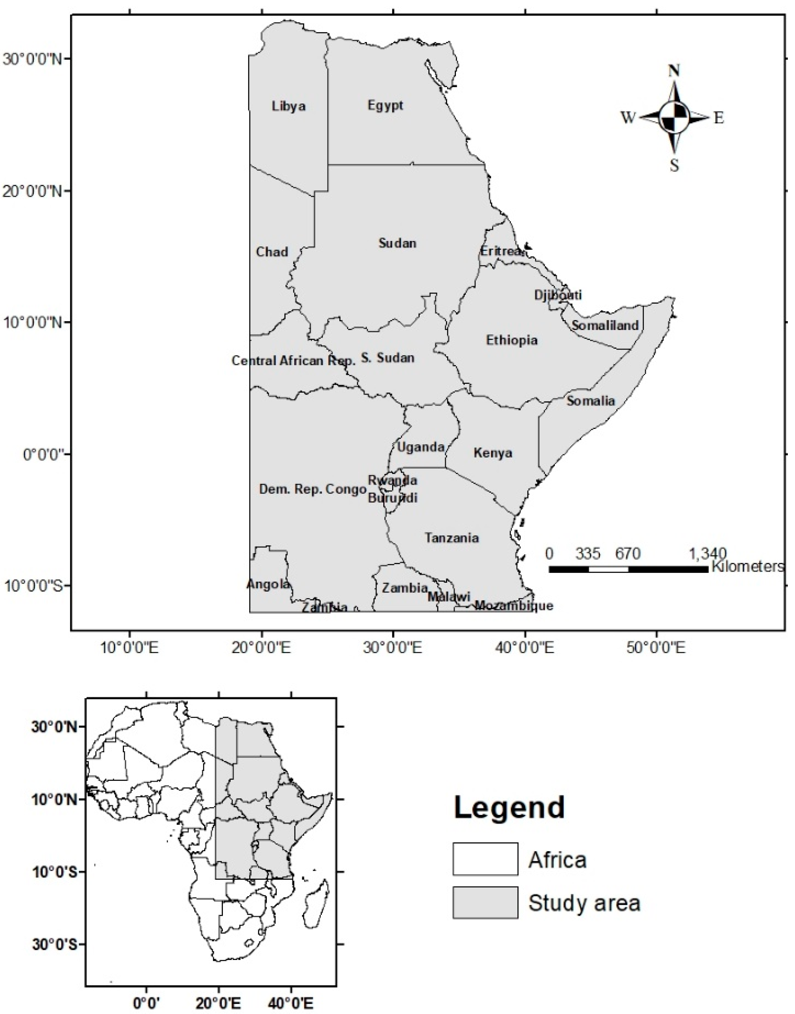
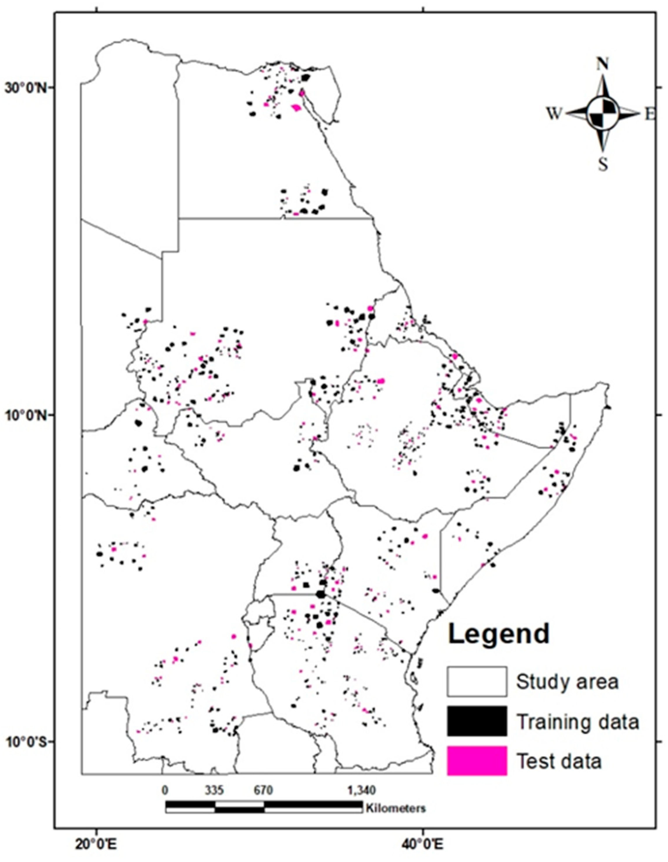
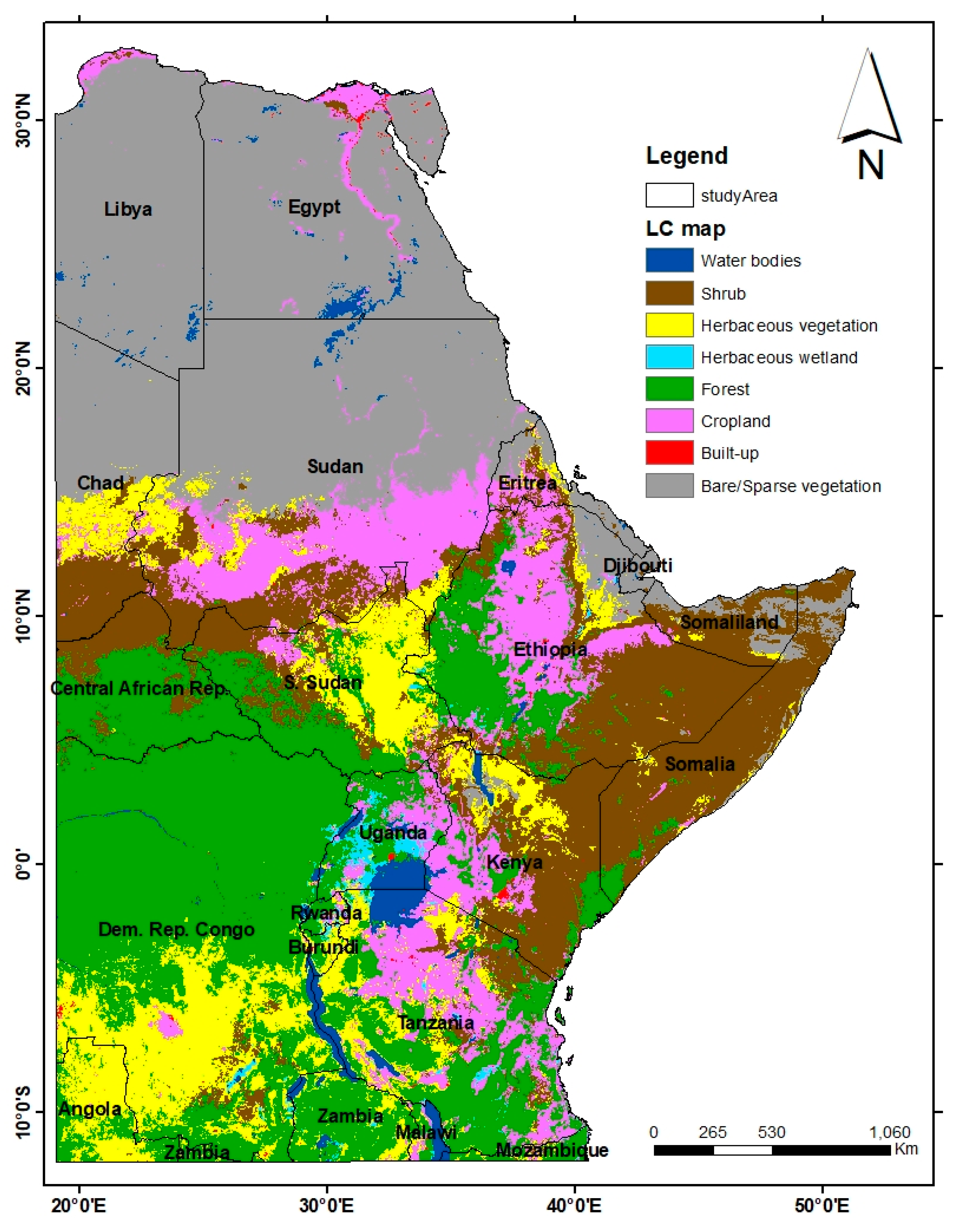
2.1. Study Area

The study area, gray-shaded region, covers approximately 30% of the total area of the African continent (Figure 1). It is found between latitude, 11°58′31.71″ S, 33°0′18.55″ N, and longitude, 19°4′35.03″ E, 51°24′37.33″ E. It includes about 18 countries, fully or partially, that occur in the eastern, central, northeastern parts of Africa. The region is characterized by three main climates such as arid, Sahelian, tropical, and equatorial; where the northern part is mostly arid that includes the Sahara, the world’s largest desert, and central Africa is known for its tropical rain forest cover.

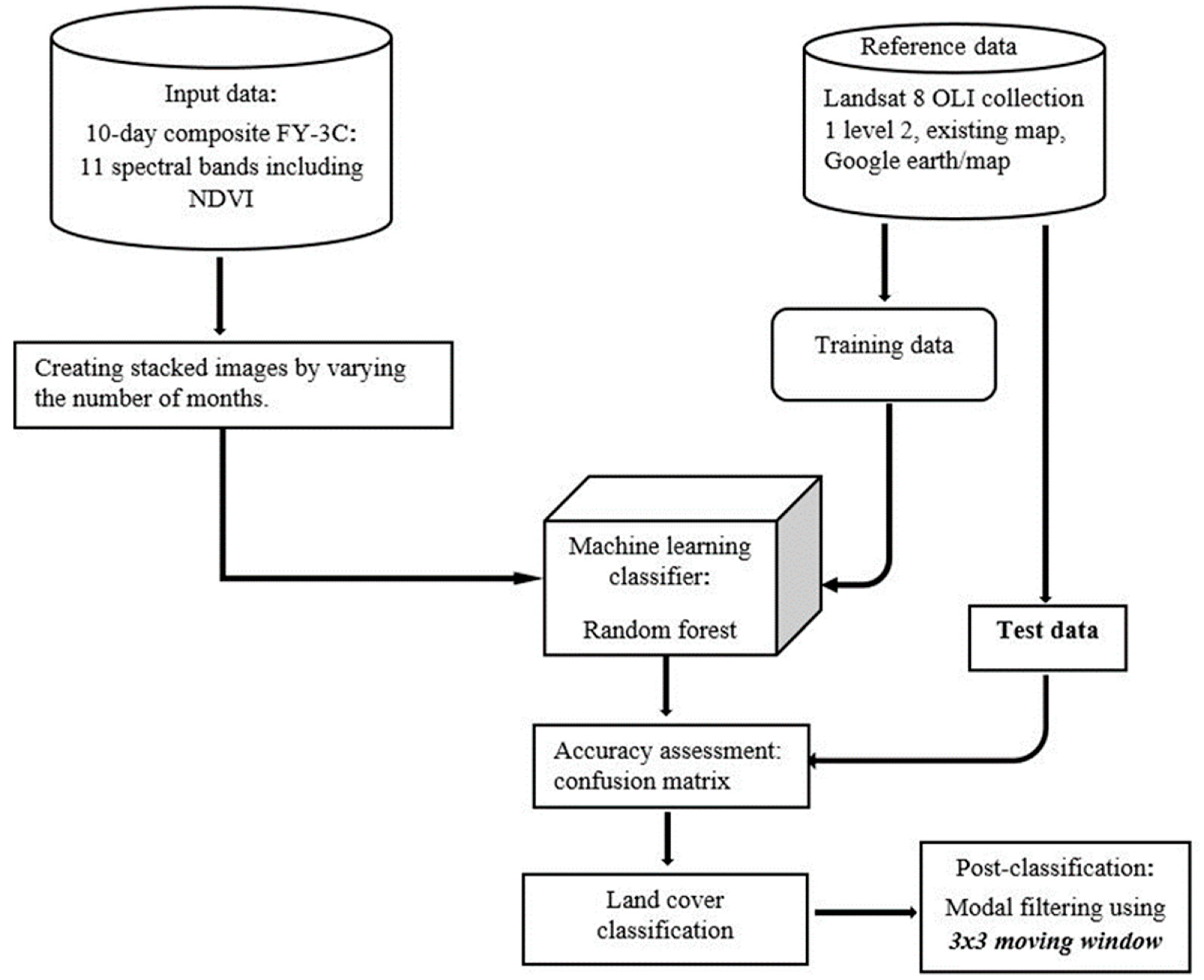
2.2. Technical Workflow

Various materials and techniques have been employed to achieve the objective of this research as discussed below and the technical route is exhibited in Figure 2.

2.3. Materials and/or Resources

Two types of satellite imageries from various sources were used for different purposes. FY-3C data are the primary input data that were acquired from the Chinese Metrological Administration (CMA). We collected one-year, 1-April 2019 to 30-March 2020, 10-day composite images with 1-km spatial resolution. Then, 11 bands, that include visible, infrared (IR), and maximum value composite (MVC) of NDVI bands, were selected to use for the intended goal (see

Table 1. List of selected bands of 10-day composite images of FY-3C.

Band No.	Name of Bands	Wavelength Range in Microm
Band 1	FY-3C_VIRR_Day_EV_RefSB	0.58–0.68
Band 2	FY-3C_VIRR_Day_EV_RefSB	0.84–0.89
Band 3	FY-3C_VIRR_Day_EV_RefSB	1.55–1.64
Band 4	FY-3C_VIRR_Day_EV_RefSB	0.43–0.48
Band 5	FY-3C_VIRR_Day_EV_RefSB	0.48–0.53
Band 6	FY-3C_VIRR_Day_EV_RefSB	0.53–0.58
Band 7	FY-3C_VIRR_Day_EV_RefSB	1.325–1.395
Band 8	FY-3C_VIRR_Day_EV_Emissive	3.55–3.93
Band 9	FY-3C_VIRR_Day_EV_Emissive	10.3–11.3
Band 10	FY-3C_VIRR_Day_EV_Emissive	11.5–12.5
Band 11	MVC value of NDVI	-

).

Landsat imageries were the other images, with higher spatial resolution than the input data, used to collect reference data. For this purpose, we acquired one-year Landsat 8 Collection 1 Level-2, which are atmospherically corrected, surface reflectance images with the same interval date as the input data. The scenes were accessed from the United States Geological Survey (USGS) website [16] by setting cloud cover criteria <10% and excluding data of unknown cloud cover. Once the images have been obtained, the best scenes were selected manually for reference sample collection for that particular location.

In addition to Landsat data, an existing map, i.e., Copernicus global discrete land cover map at 100 m resolution (CGLS LC100 discrete map) for the year 2019 (https://lcviewer.vito.be/download, accessed on 14 September 2021), Google Earth Pro and/or Google maps have also been used as a complementary and/or reference data, while collecting training and test data.

Furthermore, in order to perform various pre and post-processing of vector and raster data software such as ENVI 5.3 and ArcMap 10.7 were employed. Python 3.8 programming language was also employed to process and classify the images using machine-learning methods. To manipulate the data, we used certain Python libraries, such as Scikit learn library that includes NumPy and Matplotlib (https://scikit-learn.org/stable/, accessed on 14 September 2021); and other important packages such as osgeo, Geospatial Data Abstraction Library (gdal), ogr, geopands, and others.

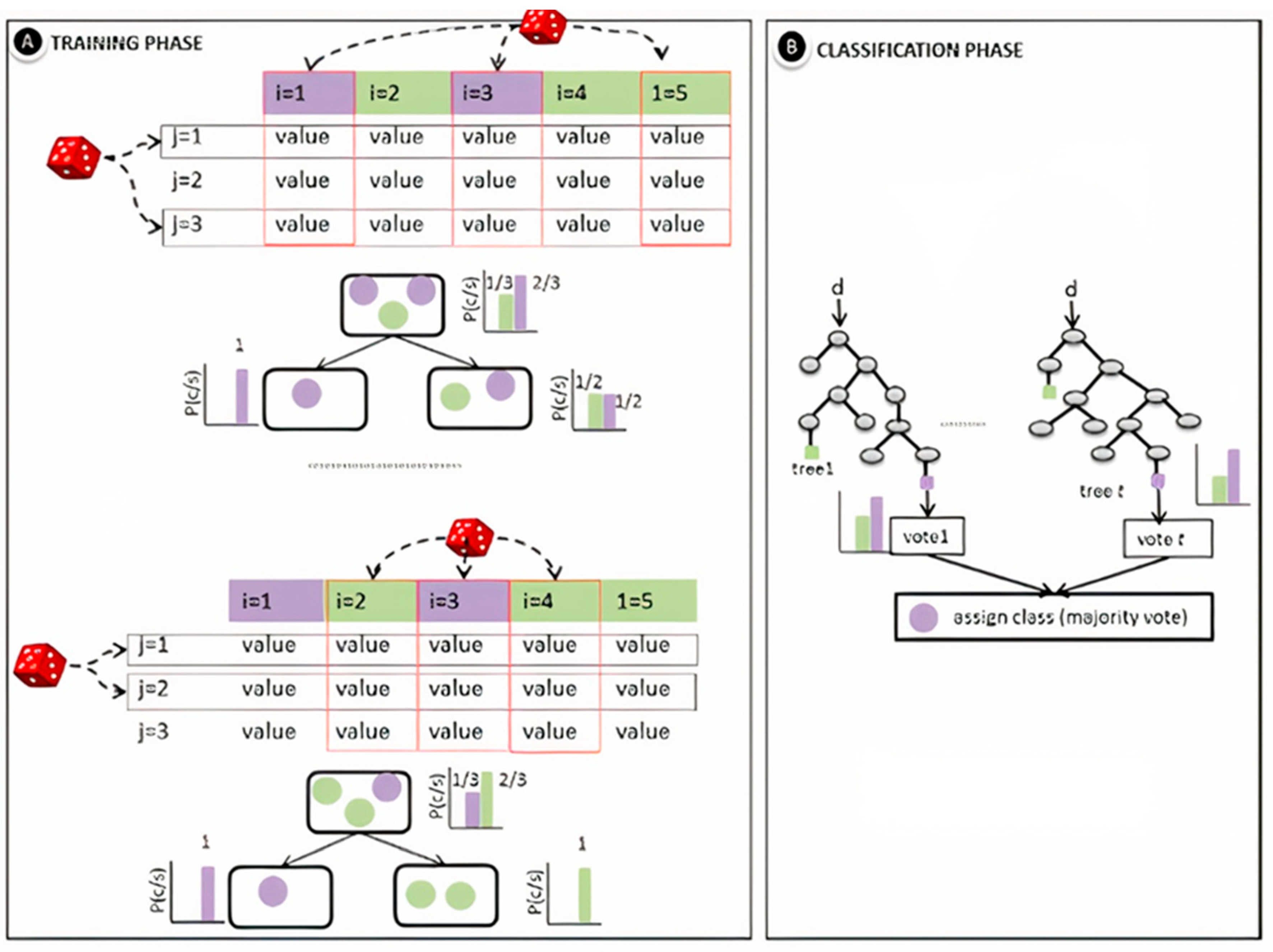
2.4. Random Forest Classifier

Machine learning algorithms are nonparametric supervised techniques that have become a major focus and a huge success in remote sensing technology in recent years, e.g., Pal and Mather [17]; Mountrakis et al. [18]; Belgiu and Drǎgut [19]; Maxwell et al. [20] and Wulder et al. [21]. Applying machine-learning algorithms provides significant benefits including the capacity to model complex class signatures, accepting a variety of input predictor data, and being unaffected by the distribution of data [20]. Several studies have found out that these methods generally yield a better result compared to traditional parametric algorithms, particularly, for complex datasets with a high-dimensional feature space, i.e., several estimator features or attributes (e.g., Friedl and Brodley [22]; Hansen and Reed [23]; Huang et al. [24]; Pal [25]; Pal and Mather [17]; Ghimire et al. [26]; Otukei and Blaschke [27]).

The random forest (RF) is an ensemble approach that consists of numerous decision trees that are formed using randomly picked predictor variables from randomly chosen training samples subsets, with class prediction based on a majority vote [19,28] (see Figure 3). It is one of the most widely applied and robust machine-learning algorithms [19].

The method of constructing a random forest is generally a combination of bagging and random subspace methods [29]. The trees are formed by drawing a subset of training samples through replacement (a bagging approach, in which case the same sample can be chosen repeatedly at the expense of the others (Figure 3A). About two-thirds of the samples (referred to as in-bag samples) are used to train the trees. Whereas, the remaining one-third (referred to as out-of-the-bag samples) are used in an internal cross-validation technique for testing the effectiveness the resulting RF model performs, or for error estimate also known as the out-of-bag (OOB) error [28,30]. Each decision tree is independently generated without any pruning and each node is split using a user-defined number of features (Mtry), selected at random. By growing the forest up to a user-defined number of trees (Ntree), the algorithm creates trees that have high variance and low bias [28]. Finally, the algorithm classifies new samples by applying majority votes obtained from several estimators (trees) [30] (Figure 3B).

Two param significantly affect the performance of the RF classifier: Ntree and Mtry [19,20]. Although various studies have shown that Mtry parameter is more important than Ntree in affecting the classification result [31,32], setting appropriate values for both param is essential to find a better accuracy. In this regard, Belgiu and Drǎgut [19] and Gislason et al. [33] suggested 500 as a default value for Ntree. Whereas, Guan et al. [34] recommended the value of Ntree as much as possible, arguing RF classifier is computationally efficient and does not overfit. Regarding Mtry parameter, it is mostly considered as the square root of the number of input variables [19,33]. On the other hand, some investigators assume Mtry as equal to the total number of exiting variables (e.g., Ghosh et al. [31]). However, such an assumption can compromise the computational efficiency, as the algorithm has to calculate the information gain resulted from all of the features used to divide the nodes [19].

A number of advantages of applying the RF algorithm have been mentioned in the literature. RF provides high accuracy [19,35], even better than several other machine learning algorithms including, discriminant analysis, support vector machines, and neural networks [30] and robust to over fitting [19,28]. It is also computationally inexpensive unlike other ensemble classifiers including support vector machine and AdaBoot. Furthermore, it enables us to select important variables [35] that allow us to remove the least significant features; and it mostly requires setting a few, two, param, i.e., Ntree and Mtry, [19,20,30] One drawback of RF is that having many trees reduces the capacity to visualize the trees [28]. In this paper, thus, we employed the RF model by setting Ntree = 500 and Mtry equals to the square root of the number of variables.

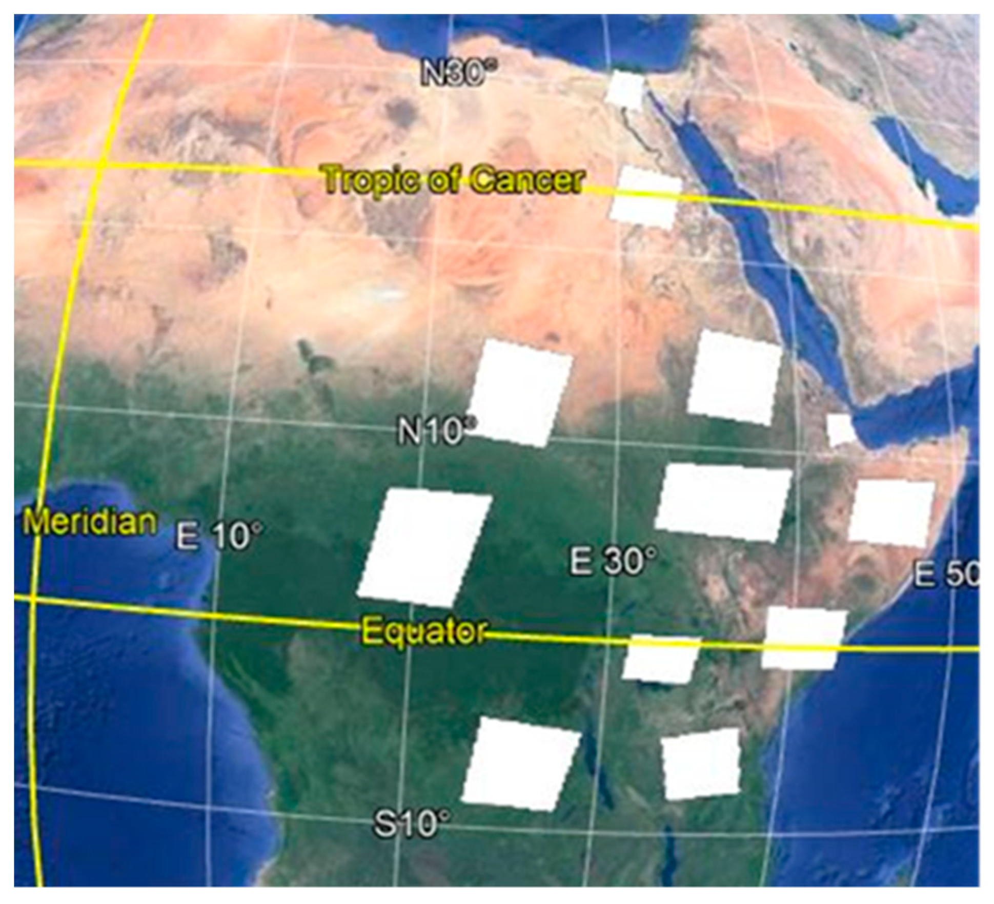
2.5. Selecting Reference Data Location and Landsat Data Acquisition

The location and distribution of the Landsat imageries for reference data collection were determined on Google Earth Pro by creating a polygon (see Figure 4) on the basis of eco-regions of Africa, previous LC maps of Africa, Copernicus global land cover, globcover, and personal experience. As shown in Figure 4, the white polygons, KMZ files format, are randomly distributed across the study area according to earlier mentioned criteria. Then, the KMZ files (location of reference data) were imported to the USGS website to select and acquire Landsat imageries.

2.6. Naming of Classes

Land cover types in the study area have been categorized into eight major classes (

Table 2. Land cover classes and their definition modified after Smets et al. [7].

Land Cover Class	Class Definition Based on UN LCCS
1. Bare/Sparse vegetation	Bare surface or land with vegetation cover no higher than 10% any time of the year
2. Built-up	Land surface covered by buildings and other man-made structures
3. Cropland	Lands that are covered with intermittent crops, harvested, and then left barren (e.g., single and multiple cropping systems). Perennial woody crops will be categorized as a forest or shrub based on the definition.
4. Forest	Lands covered by woody plants, with a percent cover of more than 15% and a height of more than 5 m. Exceptions: a woody plant having a distinct physiognomic feature of a tree can be categorized as a tree even if its height is less than 5 m but greater than 3 m.
5. Herbaceous wetland	Land covered by a persistent mixture of having water and herbaceous or woody plants. Vegetation may be found in salt, brackish, or freshwater.
6. Herbaceous vegetation	Plants that lack a distinct solid structure and have no persistent stems or shoots above the surface. It may consist of up to 10% trees and shrubs.
7. Shrubs	These are woody perennial plants, with persistent and woody stems, that are less than 5 m tall and lack a distinct main stem. The leaves of the shrub can be either evergreen or deciduous.
8. Water bodies	These include lakes, reservoirs, and rivers. The water could be fresh or salty.

) on the basis of the United Nations Land Cover Classification System (LCCS) as stated in Copernicus Global Land Operations—Lot 1 [7].

2.7. Reference Data/ROI Collection

Studies have revealed that the accuracy of land cover maps predominantly relies on the quality and quantity of reference (training and test) data. According to Huang et al. [24] training data may have a greater influence than the type of classifier employed. However, researchers recommend contradicting figures on the size of training data. For instance, Noi and Kappas [36] suggested that the training sample size should be 0.25 percent of the overall study area. Jensen and Lulla [37], whereas, proposed training pixels should be at least ten times the number of variables in the classification model. Other studies, on the other hand, found out that machine-learning algorithms required a large number of training data to achieve better results [33].

For this work, therefore, we managed to collect a large amount of reference data, 91,207 training pixels, and 27,667 test pixels, across the study area (see Figure 5) from Landsat 8 surface reflectance imageries. The number of both training and test pixels for the various classes varies according to the size of the land cover,

Table 3. Reference data per individual classes.

Class (Name)	Training Data	Test Data
	Number of Pixels per Class
Class 1 (Bare/Sparse vegetation)	20585	6424
Class 2 (Built-up)	1620	575
Class 3 (Cropland)	15472	4246
Class 4 (Forest)	11378	3101
Class 5 (Herbaceous wetland)	1686	602
Class 6 (Herbaceous vegetation)	12394	3641
Class 7 (Shrubs)	18956	5283
Class 8 (Water bodies)	9116	3795
Total number pixel	91207	27667

. Because classes that occupy vast regions require more samples than those that occupy small areas, area-proportional distribution of training samples per class produced the best classification results [38].

Before starting image interpretation to collect land cover examples, false-color composite images, mostly 5,4,3, were created from six-stacked bands (band 2 through 7) in ENVI and made to overlay exiting Copernicus map of the particular area. Then, identification and/or interpretation of the various land cover classes were carried out on the composite Landsat images by employing three techniques/references simultaneously.

These are:

• Interpretations of the images by applying image interpretation elements such as texture, pattern, association, color, tone, and others.
• Crosschecking the underlying previous land cover map, i.e., Copernicus global land cover map (100 m) if the class is homogenous for at least the minimum mapping unit (1 km × 1 km, i.e., 40 × 40 Landsat pixels) of the input data.
• Finally, further cross-checking/consolation was done on higher resolution imageries, Google Earth Pro, and Google Maps.

Generally, class naming was based on the interpretation of Landsat images aided by the previous map and Google Earth Pro/Google Maps. However, when discrepancies/disagreement among these references occurred, as happened often, naming of classes was made by referring to Google Earth Pro and/or maps as they are higher resolution imageries than the other two references. After the name of the land cover type was confirmed, the samples were annotated as polygons XML files and subsequently exported as shapefile using ENVI.

Finally, the shapefiles from the different scenes were merged in ArcMap to create a single shapefile containing all collected reference data. Then, merged single reference data were divided into two (Figure 5), using ArcMap, approximately 75/25 train/independent test data, respectively by randomly selecting 5-sample polygons out of 20-shape files from each class and exporting them. Once the selected test samples were exported as separate shapefile, they were deleted from the merged data that contain both training and test data so that the remaining data comprise only 75-percent of the sample, the training data.

As mentioned in Section 2.1, a total of one-year (1 April 2019 to 30 March 2020) 10-day composite data were considered and systematically divided into different months, following yearly seasons, so as to determine how variations in the number of months of multi temporal-data impact the land cover classification accuracy.

Accordingly, seven different types of stacked imageries were formed from eleven spectral bands including NDVI by varying the number of continuous months for the first five input data listed below and by employing feature selection/reduction methods for the last two.

• One-month stacked image (OMSI): this is created from 10-day composite images of a single month (April 2019), it consists of three composite images where each of the images is composed of 10-day scenes. As a result, one month stacked image has a total of 33-bands/features which resulted from the multiplication of three variables as follow:

  3-Images per month × 1-month × 11-bands = 33 bands/features
• Three months stacked image (TMSI): a stacked image made up of 3-month (Apr, May, and June 2019) composite images, and comprises a total of 99-band images.
• Six months stacked image (SMSI): a stacked composite image of six-month (Apr, May, June, July, August, September 2019) with 198-feature/band.
• Nine months stacked image (NMSI): it is a stacked scene of 9-month (Apr, May, Jun, Jul, August, September, October, November, December 2019) and has a total of 297-bands/features.
• One-year stacked image (OYSI): contains the maximum features/bands, 396, as it is made of one-year, 1 April 2019 to 1 April 2020, composite images.
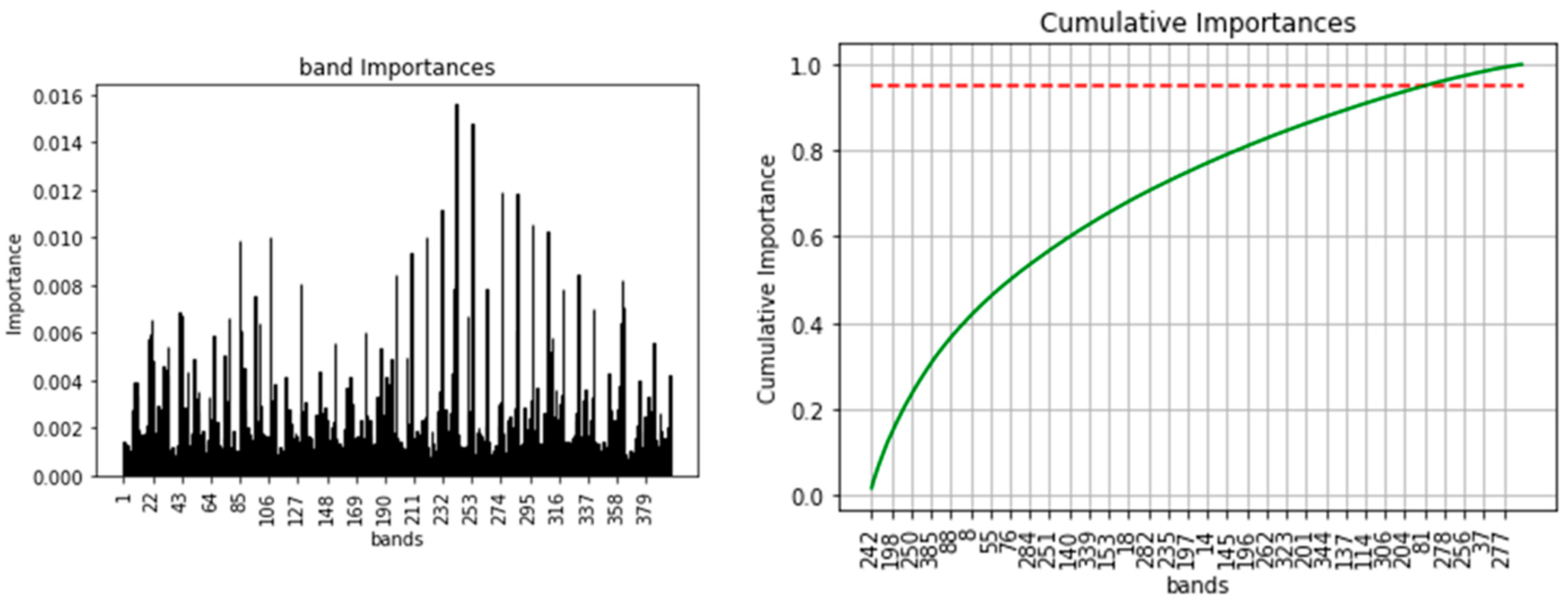
• Selected data from one-year stacked image (SDFOYSI): as the name implies the data are generated by feature selection/reduction methods using variable importance of random forest classifier. One of the advantages of using a random forest classifier is its feature/variable importance algorithm, built-in functionality that helps to select the most important variables and remove the least significant ones. Using the algorithm and by setting 95% cumulative importance, 337 features/bands were selected out of 396 features/bands of OYSI (see Figure 6). Implying the rest 59 bands are the least important features and have an insignificant effect on the overall result.
• Selected nine months stacked image (SNMSI): a stacked image consisting of selected 9-month imageries (April, May, June, July, August, September 2019; and January, Februry, and March 2020) that are created based on the result obtained by processing SMSI and NMSI. That is, it is formed from the one-year data by removing three months (October, November, December 2019) data as there is no variation in accuracy observed by processing SMSI and NMSI where the latter comprises the excluded months. In other words, it is data derived by a systematic feature selection technique.

2.8. Model Training

Data processing including model training, classification, and accuracy assessments was performed in Python 3.8 programming language platform. The software consists of various built-in libraries such as Scikit-Learn(sklearn), NumPy, and Matplotlib that enable us to execute various machine learning algorithms including random forest.

In this paper, therefore, we employed a random forest model to classify the data. The algorithm was trained using the seven different input data types discussed in Section 2.8 but using the same training dataset that consists of 91,207 training pixels. Model param were set to default values for the majority of the param as given in sklearn library except for the Ntree (n_estimator) and random state, which were converted from 100 to 500 following suggestions by Gislason et al. [33], Maxwell et al. [20], and Belgiu and Drǎgut [19], and none to 42, respectively. Regarding Mtry, we used the default value, which is equal to the square root of the number of variables; the most widely applied and suggested value by several previous works.

2.9. Accuracy Assessment

Performances of the various models that were generated by varying the input data sets were evaluated by using error matrix, the most common accuracy evaluation techniques, f-score and kappa coefficient. The error matrix is also known as the confusion matrix because it identifies not only overall errors for each category but also misclassifications (due to confusion between categories) by category. The confusion matrix allows an assessment of the user’s accuracy or recall (the number of correctly classified pixels divided by the total number of pixels predicted within that class) and producer’s accuracy also known as precision (the number of correctly classified pixels divided by the total number of pixels truly in that class) for each class [39].

3. Results

The performance of all seven input datasets composed of the different number of stacked imageries consisted of 3 to 36 composite images, where each of them containing 11 bands including NDVI was evaluated with the same independent test sample. However, the number of reference data, training, and test pixels, collected for the various classes vary according to the size of the land cover. That is, land cover types with larger areal coverage, e.g., Bare/Sparse vegetation, cropland, shrub, and forest were represented by a large number of pixels; while minority classes, such as built-up and herbaceous wetland were represented by fewer pixels in proportion with the prevalence of the class (see Figure 7 and

Table 4. Classification reports of seven different amounts of time series data (a–g).

Input Data	Class Name	Bare/Sparse Vegetation	Built-up	Cropland	Forest	Herbaceous Wetland	Herbaceous Vegetation	Shrub	Water Bodies
	Class ID	1	2	3	4	5	6	7	8
	No. of Pixels	6424	575	4246	3101	602	3641	5283	3795
(a) OMSI	precision	0.89	0.68	0.68	0.84	0.65	0.72	0.72	0.92
	recall	0.93	0.55	0.79	0.88	0.48	0.59	0.71	0.90
	f1-score	0.91	0.61	0.73	0.86	0.55	0.65	0.71	0.91
	accuracy	0.79
	kappa_score	0.75
(b) TMSI	precision	0.92	0.58	0.76	0.84	0.75	0.79	0.74	0.94
	recall	0.92	0.52	0.78	0.89	0.57	0.65	0.79	0.97
	f1-score	0.92	0.54	0.77	0.86	0.65	0.71	0.77	0.95
	accuracy	0.83
	kappa_score	0.79
(c) SMSI	precision	0.93	0.58	0.79	0.89	0.73	0.77	0.76	0.96
	recall	0.93	0.56	0.80	0.88	0.66	0.70	0.81	0.97
	f1-score	0.93	0.57	0.80	0.88	0.69	0.73	0.79	0.97
	accuracy	0.84
	kappa_score	0.81
(d) NMSI	precision	0.94	0.48	0.77	0.89	0.72	0.77	0.77	0.96
	recall	0.92	0.54	0.82	0.86	0.67	0.70	0.80	0.97
	f1-score	0.93	0.51	0.79	0.88	0.69	0.73	0.79	0.97
	accuracy	0.84
	kappa_score	0.81
(e) OYSI	precision	0.95	0.65	0.78	0.90	0.70	0.79	0.77	0.96
	recall	0.94	0.57	0.83	0.85	0.67	0.71	0.82	0.98
	f1-score	0.94	0.61	0.81	0.87	0.68	0.75	0.79	0.97
	accuracy	0.85
	kappa_score	0.82
(f) SDFOYSI	precision	0.95	0.48	0.78	0.90	0.70	0.79	0.77	0.96
	recall	0.91	0.57	0.84	0.85	0.67	0.71	0.82	0.98
	f1-score	0.93	0.52	0.81	0.88	0.69	0.75	0.80	0.97
	accuracy	0.85
	kappa_score	0.82
(g) SNMSI	precision	0.95	0.67	0.81	0.91	0.73	0.82	0.77	0.93
	recall	0.92	0.58	0.87	0.85	0.70	0.72	0.83	0.98
	f1-score	0.93	0.62	0.84	0.88	0.72	0.76	0.80	0.95
	accuracy	0.86
	kappa_score	0.83

). The strategy proved to yield the best accuracy [38].

As stated in Section 2.9 to conduct the accuracy test, therefore, the error matrix (Figure 7) along with f1-score and kappa coefficient was employed. Table 4 and Figure 7a–d depict the overall accuracy, kappa score, precision, recall, and f1-score generally increase with the increasing number of months the data comprised. Up to 6% variation in overall accuracy and notable differences of individual class accuracy between OMSI and OYSI were observed. This variation/improvement in accuracy is due to an increase in the number of months and the related number of time series data. In other words, images collected over a longer period acquire more important attributes of the various classes than scenes acquired in a lesser time interval. The more of the period the data covers, the more properties of the land cover types associated with the composition of a feature which is intrinsic and determines the spectral character of a particular object on the surface. Seasonal variation also known as phenological properties and mixing of classes could be registered and enhance discrimination of classes.

Hence, using continuous data over a longer period enables us to record the variations/changes caused by different factors thereby the different land cover types are characterized well; and that can help us to find better classification accuracy.

However, this generalization does not necessarily mean that processing a higher number of months of multi-temporal images results in better accuracy than manipulating a lesser amount of months. For example, manipulating SNMSI produced the highest accuracy (0.86) and kappa score (0.83) although it consisted of 3 months lesser data than OYSI (see Table 4 and Figure 7e,g); consequently, the data were used to produce the land cover map of the study area (Figure 8). Similarly, despite consisting of the highest time interval/data, OYSI, resulted in the second-best result, 0.85 and 0.82, accuracy and kappa value, respectively, which is similar to the outcome found by processing SDFOYSI, a lesser amount of data were obtained by using feature reduction method (see Table 4 and Figure 7e,f. Not only these, but NMSI also produced almost the same accuracy and kappa value (0.84 and 0.81) as SMSI although it has 3-month more information. These indicate the existence of redundant information that has little/no impact on the accuracy if they are removed.

4. Discussion

4.1. Effect of Feature Selection/Reduction

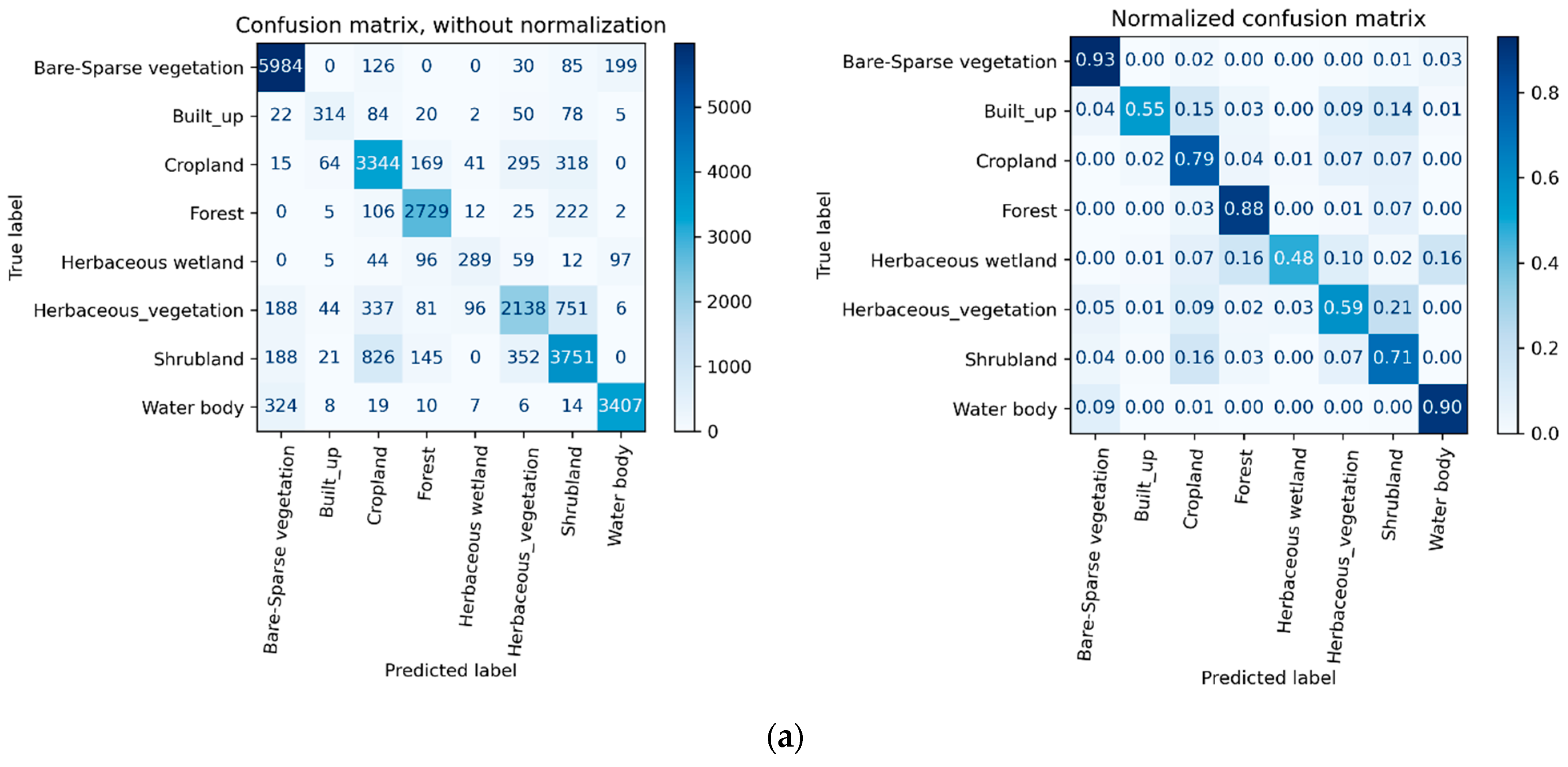
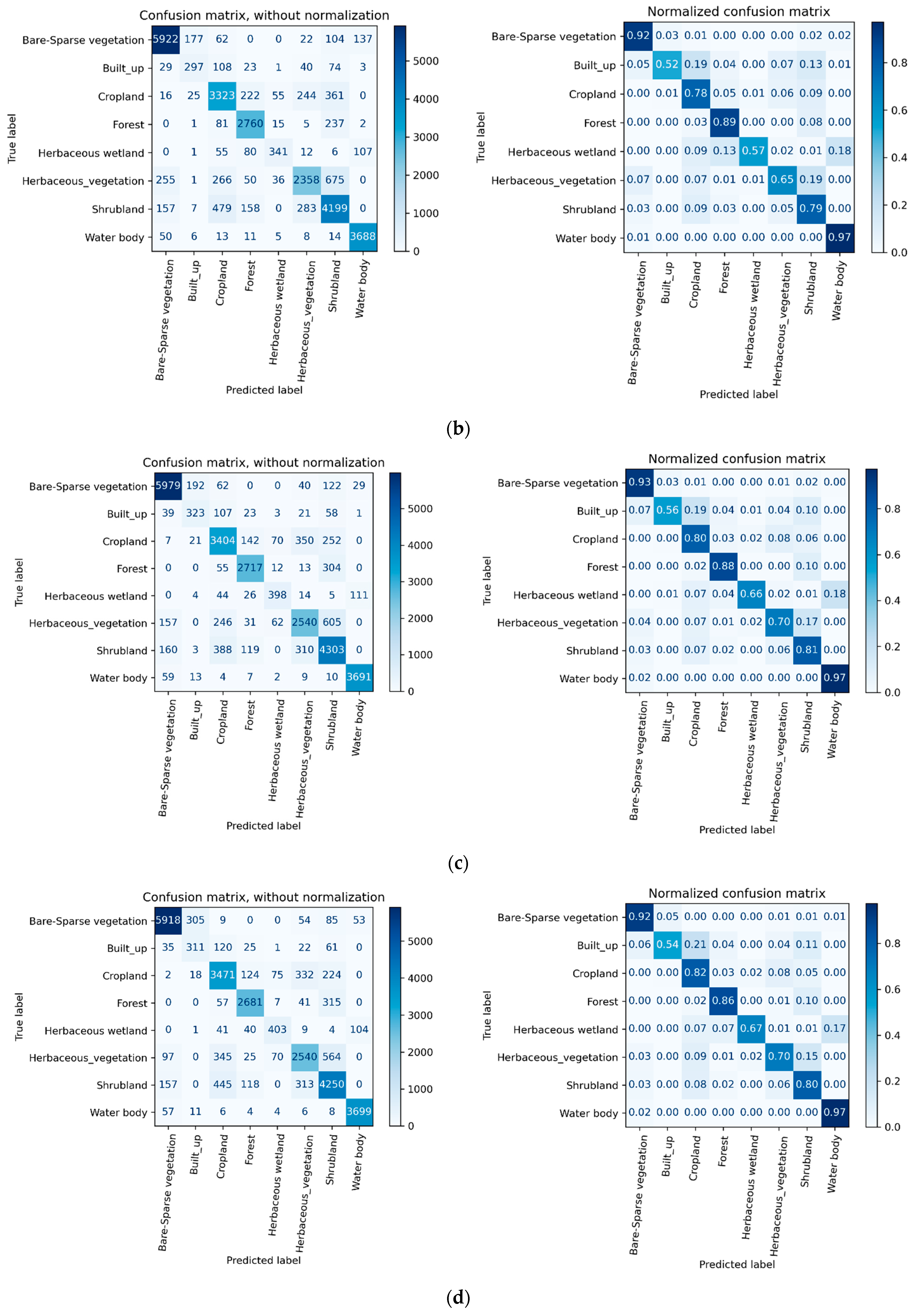
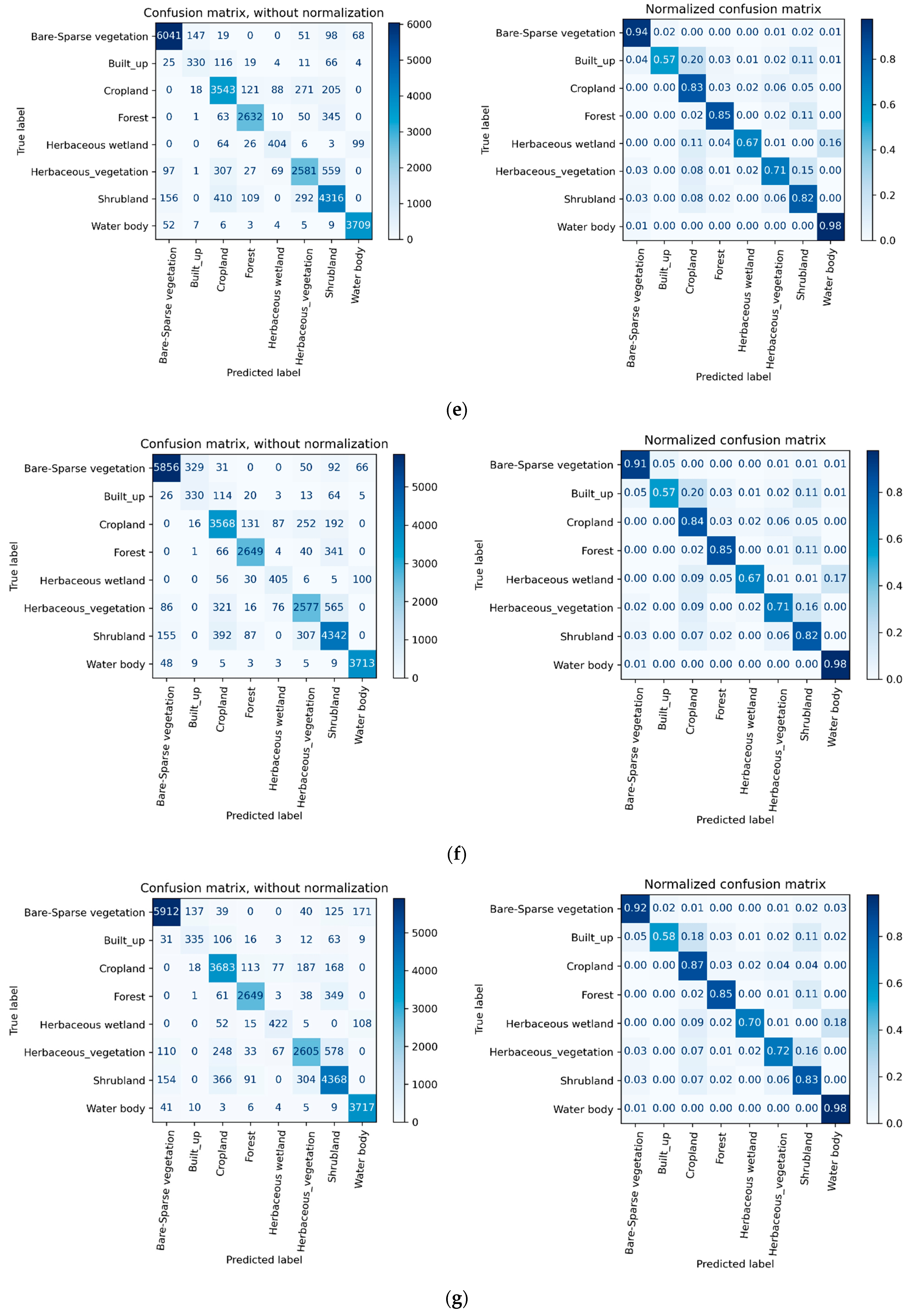
To address the redundancy of information and to remove the least significant data, two feature selection techniques have been implemented. Feature/band reduction is a method of removing the least important variables/bands without significantly altering the final product. In other words, it is a method of selecting the most vital information that represents the object [33]. It is also a means of minimizing/avoiding overfitting thereby enhancing the capacity of classifiers to generalize and reduce computational cost. In this paper, therefore, two feature selection methods, automatic and manual, were employed.

In the automatic method, we used the variable importance module of random forest in sklearn library (python 3.8) on OYSI consisted of 396 features/bands to select the most import variables; consequently, we obtained 337 features/bands using 95% cumulative importance. Analyzing the selected 337 bands resulted in almost the same accuracy and kappa score, 0.85 and 0.82, respectively, as OYSI which justified the redundancy of data that do not add vital information. Implying the rest of the 59 bands are the least important features and their effect on the overall result is insignificant.

In the second scenario, whereas, we manually created data by systematically selecting 9-month images, SNMSI, from the whole one-year images. That is, it was formed by leaving out the three continuous month images containing redundant information, based on the earlier experiment. The selected data yielded the best result and the highest accuracy (0.86), kappa score (0.83), and the best precision, recall, and f1-score (Table 4 and Figure 7g). The result infers that incorporating several features/variables with similar information negatively affects the overall accuracy and individual classes’ accuracy as it may lead to overfitting that affects the ability of the algorithm to generalize. In other words, a high number of data features (i.e., bands) might yield lesser classification accuracy than a subset of those variables, especially if the variables in the subset are selected in a certain way to focus on those that are highly relevant in differentiating the classes [20].

4.2. Error Matrix

Figure 7 shows water bodies and bare/sparse vegetation are the most accurately classified classes, above 0.9, and little variations in recall and f1-score for all types of input data. These indicate that the classes have distinct spectral properties that are affected only slightly by the change in the number of months/temporal data processed; seasonal variation has little impact on them. On the other hand, the accuracy (user’s, producers, and f1-score) of four vegetation classes such as cropland, herbaceous wetland, herbaceous vegetation, and shrub improves by at least by 1% with increasing the number of months/temporal data, implying the significant impact of phenological event variation in surface cover type. Built-up area, however, showed no pattern with changes in the number of months as it is independent of seasonal variation. Moreover, it was classified with the least classification accuracy barely above 60%; and it is highly confused with cropland. This could be caused by the mixed pixels as the two classes are spatially associated and found mixed in most cases. Mixed pixel is one of the main factors that affect land cover accuracy when coarse resolution imageries are used [2]. The other reason could be its size. Since it is a minority class, found covering a small area, it is difficult to collect a large amount of reference data. Similarly, herbaceous wetland and herbaceous vegetation were mapped with less accuracy. The former is due to its size, being a minority class, and exhibiting similar spectral properties with water body, cropland, and forest; and/or they have mixed pixels of these classes. As a result, it was often mislabeled to these classes. Regarding herbaceous vegetation, it was mostly misclassified as shrub and cropland. In addition to the reasons mentioned above, that could be attributed to class/legend definition. That is, herbaceous vegetation can contain up to 10% trees and/or shrubs by definition, so it is highly likely to misclassify mixed classes where one of the classes is dominant and the other is close to the cut-off value. For instance, land covered by 87% herbaceous vegetation and 13% trees/shrubs may be misinterpreted as herbaceous vegetation while collecting data as the method of gathering information is a visual inspection which is prone to error that ultimately leads to confusion and misclassification. This could also be the main reason for the misclassification of shrubs as forest and vise verse. The impact of land cover class definition on accuracy has also been reported by [7].

5. Conclusions

The objectives of this work were to analyze the effect of processing various amounts of months of multi-temporal satellite data on the accuracy of a land cover classification and to produce a land cover map of parts of Africa using the best-input data and machine learning, random forest, classifier. We also aimed to evaluate/assess the effectiveness of FY-3C Chinese metrological satellite data in mapping the land cover of Africa.

Stepwise experimentations were carried out by increasing the number of months, i.e., temporal data. We started with a one-month stacked image comprised of three 10-day composite scenes where each scene has 11-band including the average maximum NDVI and 1 km spatial resolution; and then increased the number of the month by three, six, nine, and twelve. The months were set to be consecutive beginning from April 2019 to March 2020 and divided considering the four annual seasons. In addition, two different input data sets were generated by the band selection/reduction method from the one-year data that makes the total amount of input data sets seven. For all input data sets, a random forest algorithm was trained using the same training samples (91207 training pixels), but different quantities for each class, that were collected from Landsat imageries. Finally, all the input data were tested against the same independent test samples that consist of 27667-pixel.

The overall accuracy, kappa coefficient, and individual class accuracy generally increase with increasing the number of continuous time-series data/months. However, the best result was not achieved by manipulating one-year stacked multi-temporal data despite consisting of the maximum months/input data. Using this data only yielded the second-best accuracy (0.85) which is the same as the accuracy resulting from processing data obtained after feature selection/reduction on one-year data. The highest accuracy, both overall accuracy (0.86) and kappa coefficient (0.83) were attained when systematically selected 9-month imageries, three seasons, were processed; consequently, the data were chosen to create the land cover map of the study area.

In large area land cover mapping, employing a systematic selection of months and/or features from one-year multi-temporal data allows us to achieve the best result. Moreover, conducting variable selection using 95% cumulative importance over one-year data had little/no impact on the overall accuracy although significant bands (59) were discarded.

In this study, therefore, despite using a single input data type from FY-3C, high overall accuracy was attained, above 85%, suggesting FY-3 data are highly effective and suitable for land cover classification of Africa.

Finally, better classification accuracy can be reached if the spatial resolution of the input data are improved and other ancillary input data are considered. In addition, increasing spatial resolution would decrease pixel mixture that in turn enhances differentiability among classes; especially minority classes could be mapped with better accuracy. On the other hand, the overall accuracy decreases if the thematic resolution, the number of classes, increases [5,21].

References

1. Tchuenté, A.T.K.; Roujean, J.-L.; De Jong, S. Comparison and relative quality assessment of the GLC2000, GLOBCOVER, MODIS and ECOCLIMAP land cover data sets at the African continental scale. Int. J. Appl. Earth Obs. Geoinf. 2011, 13, 207–219. [Google Scholar] [CrossRef]
2. Cihlar, J. Land Cover Mapping of Large Areas from Satellites: Status and Research Priorities. Int. J. Remote Sens. 2000, 21, 1093–1114. [Google Scholar] [CrossRef]
3. Beaubien, J.; Cihlar, J.; Simard, G.; Latifovic, R. Land cover from multiple thematic mapper scenes using a new enhancement-classification methodology. J. Geophys. Res. Atmos. 1999, 104, 27909–27920. [Google Scholar] [CrossRef]
4. Foody, G.M. Status of land cover classification accuracy assessment. Remote Sens. Environ. 2002, 80, 185–201. [Google Scholar] [CrossRef]
5. Latifovic, R.; Olthof, I. Accuracy assessment using sub-pixel fractional error matrices of global land cover products derived from satellite data. Remote. Sens. Environ. 2004, 90, 153–165. [Google Scholar] [CrossRef]
6. Friedl, M.; McIver, D.; Hodges, J.; Zhang, X.; Muchoney, D.; Strahler, A.; Woodcock, C.; Gopal, S.; Schneider, A.; Cooper, A.; et al. Global land cover mapping from MODIS: Algorithms and early results. Remote Sens. Environ. 2002, 83, 287–302. [Google Scholar] [CrossRef]
7. Smets, B.; Buchhorn, M.; Lesiv, M.; Tsendbazar, N.-E. Copernicus Global Land Operations “Vegetation and Energy”; Copernicus: Brussels, Belgium, 2017; Volume 1. [Google Scholar]
8. Cihlar, J.; Ly, H.; Xiao, Q. Land cover classification with AVHRR multichannel composites in northern environments. Remote Sens. Environ. 1996, 58, 36–51. [Google Scholar] [CrossRef]
9. Campbell, M.; Congalton, R.G.; Hartter, J.; Ducey, M. Optimal Land Cover Mapping and Change Analysis in Northeastern Oregon Using Landsat Imagery. Photogramm. Eng. Remote. Sens. 2015, 81, 37–47. [Google Scholar] [CrossRef] [Green Version]
10. Loveland, T.R.; Belward, A.S. The IGBP-DIS global 1km land cover data set, DISCover: First results. Int. J. Remote Sens. 1997, 18, 3289–3295. [Google Scholar] [CrossRef]
11. Tang, Y.Q.; Zhang, J.S.; Wang, J.S. FY-3 meteorological satellites and the applications. China J. Space Sci. 2014, 34, 703–709. [Google Scholar]
12. Yang, Z.; Zhang, P.; Gu, S.; Hu, X.; Tang, S.; Yang, L.; Xu, N.; Zhen, Z.; Wang, L.; Wu, Q.; et al. Capability of Fengyun-3D Satellite in Earth System Observation. J. Meteorol. Res. 2019, 33, 1113–1130. [Google Scholar] [CrossRef]
13. Xu, N.; Niu, X.; Hu, X.; Wang, X.; Wu, R.; Chen, S.; Chen, L.; Sun, L.; Ding, L.; Yang, Z.; et al. Prelaunch Calibration and Radiometric Performance of the Advanced MERSI II on FengYun-3D. IEEE Trans. Geosci. Remote Sens. 2018, 56, 4866–4875. [Google Scholar] [CrossRef]
14. Yang, Z.; Lu, N.; Shi, J.; Zhang, P.; Dong, C.; Yang, J. Overview of FY-3 Payload and Ground Application System. IEEE Trans. Geosci. Remote. Sens. 2012, 50, 4846–4853. [Google Scholar] [CrossRef]
15. Han, X.; Yang, J.; Tang, S.; Han, Y. Vegetation Products Derived from Fengyun-3D Medium Resolution Spectral Imager-II. J. Meteorol. Res. 2020, 34, 775–785. [Google Scholar] [CrossRef]
16. USGS. Available online: https://earthexplorer.usgs.gov/ (accessed on 29 April 2021).
17. Pal, M.; Mather, P.M. Support vector machines for classification in remote sensing. Int. J. Remote. Sens. 2005, 26, 1007–1011. [Google Scholar] [CrossRef]
18. Mountrakis, G.; Im, J.; Ogole, C. Support vector machines in remote sensing: A review. ISPRS J. Photogramm. Remote Sens. 2010, 66, 247–259. [Google Scholar] [CrossRef]
19. Belgiu, M.; Drǎgut, L. Random forest in remote sensing: A review of applications and future directions. ISPRS J. Photogramm. Remote Sens. 2016, 114, 24–31. [Google Scholar] [CrossRef]
20. Maxwell, A.E.; Warner, T.A.; Fang, F. Implementation of machine-learning classification in remote sensing: An applied review. Int. J. Remote Sens. 2018, 39, 2784–2817. [Google Scholar] [CrossRef] [Green Version]
21. Wulder, M.A.; Coops, N.C.; Roy, D.P.; White, J.C.; Hermosilla, T. Land cover 2.0. Int. J. Remote Sens. 2018, 39, 4254–4284. [Google Scholar] [CrossRef] [Green Version]
22. Friedl, M.A.; Brodley, C.E. Decision tree classification of land cover from remotely sensed data. Remote Sens. Environ. 1997, 61, 399–409. [Google Scholar] [CrossRef]
23. Hansen, M.C.; Reed, B.W. A comparison of the IGBP DISCover and University of Maryland 1 km global land cover products. Int. J. Remote Sens. 2000, 21, 1365–1373. [Google Scholar] [CrossRef]
24. Huang, C.; Davis, L.S.; Townshend, J.R.G. An assessment of support vector machines for land cover classification. Int. J. Remote Sens. 2002, 23, 725–749. [Google Scholar] [CrossRef]
25. Pal, M. Random forest classifier for remote sensing classification. Int. J. Remote Sens. 2005, 26, 217–222. [Google Scholar] [CrossRef]
26. Ghimire, B.; Rogan, J.; Rodriguez-Galiano, V.F.; Panday, P.; Neeti, N. An Evaluation of Bagging, Boosting, and Random Forests for Land-Cover Classification in Cape Cod, Massachusetts, USA. GISci. Remote Sens. 2012, 49, 623–643. [Google Scholar] [CrossRef]
27. Otukei, J.R.; Blaschke, T. Land cover change assessment using decision trees, support vector machines and maximum likelihood classification algorithms. Int. J. Appl. Earth Obs. Geoinf. 2010, 12S, S27–S31. [Google Scholar] [CrossRef]
28. Breiman, L. RandomForests. Mach. Learn. 2001, 45, 5–32. [Google Scholar] [CrossRef] [Green Version]
29. Tso, B.; Mather, P. Classification Methods for Remotely Sensed Data; CRC Press: Boca Raton, FL, USA, 2009; p. 367. [Google Scholar]
30. Liaw, A.; Wiener, M. Classification and regression by randomForest. R News 2002, 2, 18–22. [Google Scholar]
31. Ghosh, A.; Fassnacht, F.E.; Joshi, P.K.; Koch, B. A framework for mapping tree species combining hyperspectral and LiDAR data: Role of selected classifiers and sensor across three spatial scales. Int. J. Appl. Earth Obs. Geoinf. 2014, 26, 49–63. [Google Scholar] [CrossRef]
32. Kulkarni, V.Y.; Sinha, P.K. Pruning of random forest classifiers: A survey and future directions. In Proceedings of the 2012 International Conference on Data Science & Engineering (ICDSE), Kerala, India, 18–20 July 2012. [Google Scholar]
33. Gislason, P.O.; Benediktsson, J.A.; Sveinsson, J.R. Random Forests for land cover classification. Pattern Recognit. Lett. 2006, 27, 294–300. [Google Scholar] [CrossRef]
34. Guan, H.; Li, J.; Chapman, M.; Deng, F.; Ji, Z.; Yang, X. Integration of orthoimagery and lidar data for object-based urban thematic mapping using random forests. Int. J. Remote Sens. 2013, 34, 5166–5186. [Google Scholar] [CrossRef]
35. Rodriguez-Galiano, V.F.; Ghimire, B.; Rogan, J.; Olmo, M.C.; Rigol-Sanchez, J.P. An assessment of the effectiveness of a random forest classifier for land-cover classification. ISPRS J. Photogramm. Remote Sens. 2012, 67, 93–104. [Google Scholar] [CrossRef]
36. Noi, P.T.; Kappas, M. Comparison of Random Forest, k-Nearest Neighbor, and Support Vector Machine Classifiers for Land Cover Classification Using Sentinel-2 Imagery. Sensors 2018, 18, 18. [Google Scholar]
37. Jensen, J.R.; Lulla, K. Introductory digital image processing: A remote sensing perspective. Geocarto Int. 1987, 2, 65. [Google Scholar] [CrossRef]
38. Colditz, R.R. An Evaluation of Different Training Sample Allocation Schemes for Discrete and Continuous Land Cover Classification Using Decision Tree-Based Algorithms. Remote Sens. 2015, 7, 9655–9681. [Google Scholar] [CrossRef] [Green Version]
39. Campbell, J.B.; Wynne, R.H. Introduction to Remote Sensing, 5th ed.; The Guilford Press: New York, NY, USA, 2011; p. 718. [Google Scholar]
Figure 1. Map of the study area, gray shaded region, and its location in Africa.
Remotesensing 13 04461 g001
Figure 2. Technical workflow.
Remotesensing 13 04461 g002
Figure 3. Training and classification phases of Random Forest classifier: i = samples, j = variables, p =probability, c = class, s = data, t = number of trees, d = new data to be classified, and value = the different values that the variable j can have [19].
Remotesensing 13 04461 g003
Figure 4. Location and distribution of Landsat imageries, white polygons, for reference data collection.
Remotesensing 13 04461 g004
Figure 5. Distribution of training and test data.2.8. Pre-processing of FY-3C 10-day composite data.
Remotesensing 13 04461 g005
Figure 6. Band importance (left) and 95% cumulative importance (right).
Remotesensing 13 04461 g006
Figure 7. Confusion matrix of the various amount of months. (a) Confusion matrix of OMSI; (b) Confusion matrix of TMSI; (c) Confusion matrix of SMSI; (d) Confusion matrix of NMSI; (e) Confusion matrix of OYSI; (f) Confusion matrix of SDFOYSI; (g) Confusion matrix of SNMSI.
Remotesensing 13 04461 g007aRemotesensing 13 04461 g007bRemotesensing 13 04461 g007c
Figure 8. Land cover map of the study area.
Remotesensing 13 04461 g008