Abstract
Emissivity information derived from thermal infrared (TIR) hyperspectral imagery has the advantages of both high spatial and spectral resolutions, which facilitate the detection and identification of the subtle spectral features of ground targets. Despite the emergence of several different TIR hyperspectral imagers, there are still no universal spectral emissivity measurement standards for TIR hyperspectral imagers in the field. In this paper, we address the problems encountered when measuring emissivity spectra in the field and propose a practical data acquisition and processing framework for a Fourier transform (FT) TIR hyperspectral imager—the Hyper-Cam LW—to obtain high-quality emissivity spectra in the field. This framework consists of three main parts. (1) The performance of the Hyper-Cam LW sensor was evaluated in terms of the radiometric calibration and measurement noise, and a data acquisition procedure was carried out to obtain the useful TIR hyperspectral imagery in the field. (2) The data quality of the original TIR hyperspectral imagery was improved through preprocessing operations, including band selection, denoising, and background radiance correction. A spatial denoising method was also introduced to preserve the atmospheric radiance features in the spectra. (3) Three representative temperature-emissivity separation (TES) algorithms were evaluated and compared based on the Hyper-Cam LW TIR hyperspectral imagery, and the optimal TES algorithm was adopted to determine the final spectral emissivity. These algorithms are the iterative spectrally smooth temperature and emissivity separation (ISSTES) algorithm, the improved Advanced Spaceborne Thermal Emission and Reflection Radiometer temperature and emissivity separation (ASTER-TES) algorithm, and the Fast Line-of-sight Atmospheric Analysis of Hypercubes-IR (FLAASH-IR) algorithm. The emissivity results from these different methods were compared to the reference spectra measured by a Model 102F spectrometer. The experimental results indicated that the retrieved emissivity spectra from the ISSTES algorithm were more accurate than the spectra retrieved by the other methods on the same Hyper-Cam LW field data and had close consistency with the reference spectra obtained from the Model 102F spectrometer. The root-mean-square error (RMSE) between the retrieved emissivity and the standard spectra was 0.0086, and the spectral angle error was 0.0093.
1. Introduction
Compared to the reflective spectral range between 0.35 and 2.5 μm, the radiant energy of ground objects from the thermal infrared (TIR) atmospheric window of 8–12 μm is mainly self-emission energy, which is related to a material’s molecular structure and vibration [1]. Because the land surface emissivity (LSE) represents the material-intrinsic property and contains the material composition information, retrieving accurate LSE from TIR remote sensing data plays a very important role in many remote sensing applications, such as geological mapping [2,3], object identification [4,5], and land-cover classification [6,7]. Since the launch of the Heat Capacity Mapping Mission in 1978, which provided thermal imagery, much attention has been paid to the development of TIR instruments [8,9,10]. To date, various TIR imaging sensors with different spatial and spectral resolutions have been used to obtain remote sensing observations. The typical spaceborne TIR systems are Gaofen 5 (GF-5), the Advanced Spaceborne Thermal Emission and Reflection Radiometer (ASTER), Landsat 8, and the Moderate Resolution Imaging Spectroradiometer (MODIS), which provide TIR data with resolutions of 40, 90, 100, and 1000 m, respectively. Correspondingly, a number of LSE retrieval methods have been proposed for these spaceborne sensors [11,12,13,14,15]. However, because the band number of most of the LSE products from these spaceborne sensors is less than six channels, the emissivity spectra cannot highlight subtle spectral features.
With the maturation of hyperspectral imaging technology in the TIR range, there are now some commercial TIR hyperspectral imagers available for acquiring TIR hyperspectral data via airborne or field-based measurements [16]. Popular examples are the Spatially Enhanced Broadband Array Spectrograph System (SEBASS) [17], the Thermal Airborne Spectrographic Imager 600 (TASI-600) [18], and the Hyper-Cam LW sensor [19]. Differing from the multispectral TIR imagers carried on board satellites, hyperspectral TIR imagers have a greatly improved spectral resolution. In theory, the ability to acquire abundant continuous narrow bands is greatly conducive to obtaining more accurate and fine LSE spectra. Generally speaking, field-based measurement and airborne remote sensing retrieval are the two main ways of obtaining LSE information [20,21]. However, due to the cost and complicated imaging conditions of airborne platforms, it is difficult to obtain accurate LSE spectra and satisfy the demands of building an emissivity spectra library. In contrast, the field-based LSE measurement approach is able to obtain a higher LSE accuracy and comes with a lower cost. Moreover, field-measured LSE can act as the validation standard for the retrieval results from airborne platforms. Therefore, high-quality LSE measurement in the field is a fundamental and important task in remote sensing. Over the past few years, many attempts have been made to extract high-quality LSE from hyperspectral TIR data at the ground level. In 1996, the µFTIR spectrometer was developed for field emissivity measurements, and it was used to build the Johns Hopkins University (JHU) spectral library [22]. In-depth field measurement procedures and processing protocols have also been designed and published for the non-imaging Model 102F spectrometer [23,24]. Currently, non-imaging spectrometers constitute the mainstream approach for field emissivity measurement. In contrast, as reported by many studies [25,26,27], TIR hyperspectral imagers, as a new measurement means, are mostly used indoors to measure precise emissivity or evaluate design performance. Although hyperspectral TIR imagers have the advantage of both high spectral and spatial resolutions, there are still no universal spectral emissivity measurement standards for use in the field.
Differing from stable indoor measurement conditions, the environmental radiance in field conditions is affected by both the atmosphere and surrounding objects, and it can rapidly change with time, resulting in poor data quality [28]. Data quality is also directly related to measuring instruments’ performance, i.e., radiometric calibration and measurement noise [29]. However, to date, few studies have analyzed the performance of TIR hyperspectral imagers in extracting accurate spectral emissivity with a specific instrument parameter configuration. Therefore, it is imperative to quantitatively evaluate instrument performance before a field measurement campaign and to conduct a data acquisition procedure in the field to acquire useful TIR hyperspectral imagery. In addition, compared to the data obtained by non-imaging spectrometers, TIR hyperspectral imagery often contain a high noise level, and previous studies [30,31,32,33] have shown that measurement noise can have a great influence on final emissivity estimations. Spectral filtering methods [18,34] have been effectively applied to the denoising of multispectral TIR data in order to improve image quality. For multispectral data, the relatively wide bandwidth makes the atmospheric components smooth, and the spectral fluctuations are mainly caused by noise. Spectral filter methods are generally applicable for denoising multispectral data with a relatively wide bandwidth. However, for hyperspectral data, filtering methods are prone to destroying the atmospheric features. A suitable temperature-emissivity separation (TES) algorithm is a key factor in obtaining final emissivity spectra of accurate shape and magnitude. To date, many TES algorithms have been proposed for use with TIR hyperspectral imagery [8,35,36,37,38,39,40,41], such as the iterative spectrally smooth temperature and emissivity separation (ISSTES) algorithm, the improved Advanced Spaceborne Thermal Emission and Reflection Radiometer temperature and emissivity separation (ASTER-TES) algorithm, and the Fast Line-of-sight Atmospheric Analysis of Hypercubes-IR (FLAASH-IR) algorithm. However, these methods were initially designed based on specific sensor data, and the performance of most of the methods, except for FLAASH-IR, has not been investigated and evaluated on Hyper-Cam LW TIR hyperspectral imagery with a specific configuration. Unlike most spectral splitting imagers, the Hyper-Cam LW sensor is the only commercially available Fourier transform (FT)-TIR hyperspectral imager on the market. It was developed by Telops Inc. (Quebec City, Canada) and can provide high spatial and spectral resolution information for infrared targets and scenes.
In this study, our aim was to develop a practical data acquisition and processing framework for the Hyper-Cam LW sensor in order to obtain high-quality emissivity spectra in the field, as shown in Figure 1. The main contributions are summarized as follows:
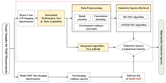
Figure 1.
The framework for deriving emissivity spectra from the Hyper-Cam LW field-based imagery.
- (1)
- A practical data measurement and processing framework was specifically proposed for the Hyper-Cam LW sensor that includes four aspects: the performance validation of the Hyper-Cam LW sensor, a field-based acquisition procedure for TIR hyperspectral imagery, data preprocessing to improve the original data quality, and appropriate TES algorithm selection via the comparison of three representative methods.
- (2)
- Data improvement was performed through band selection, imagery denoising, and environmental correction. In addition, according to the analysis of the noise distribution type and magnitude, a spatial denoising method based on Gaussian template convolution was adopted to preserve the atmospheric radiance features in the spectrum.
- (3)
- Three widely used TES algorithms were investigated and compared using Hyper-Cam LW field-measured TIR hyperspectral imagery, and the optimal TES method was selected to determine the final high-quality emissivity spectra that were quantitatively evaluated using the standard spectra measured by the Model 102F spectrometer.
The rest of this article is organized as follows. Section 2 introduces the instrument testing and data acquisition. Section 3 describes the details of the data preprocessing, including the spatial denoising method. Section 4 describes the investigation conducted using three representative TES algorithms on the field-measured Hyper-Cam LW imagery. The evaluation and analysis of the results are presented in Section 5, and our conclusions and future work are summarized in Section 6.
2. Instrument Testing and Data Acquisition
2.1. Instrumentation and Configuration
The Hyper-Cam LW sensor is the only available commercial FT-TIR hyperspectral imager on the market [26]. The spectral resolution of the Hyper-Cam LW sensor is adjustable and can reach 0.25 cm−1, and its instantaneous field-of-view (IFOV) is 0.35 mrad, leading to very high spectral and spatial resolutions. The specific configuration for field data acquisition is listed in Table 1. In our instrument testing, a modified optical lens was used to maintain consistency with the airborne nadir observations.

Table 1.
Basic specifications and configuration of the Hyper-Cam LW sensor for field-based TIR hyperspectral imagery acquisition.
2.2. Instrument Performance Testing
The radiometric calibration quality and noise level are generally different among different sensors and have large effects on the retrieval accuracy of emissivity spectra [42]. The performance of the radiometric calibration and noise level were assessed in the laboratory, as shown in Figure 2.
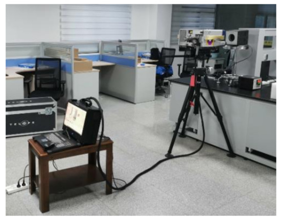
Figure 2.
Instrument performance testing in the laboratory: the control computer (left), the Hyper-Cam LW sensor, and the temperature-tunable blackbody (right).
2.2.1. Radiometric Calibration and Stability Testing
The scene radiance measured by the sensor was converted into the instrument response values. This process can be formulated as follows:
where is the instrument linear response coefficient, is the radiance emitted from the measurement scene, is the instrument self-emission with temperature , and is the instrument response digital number.
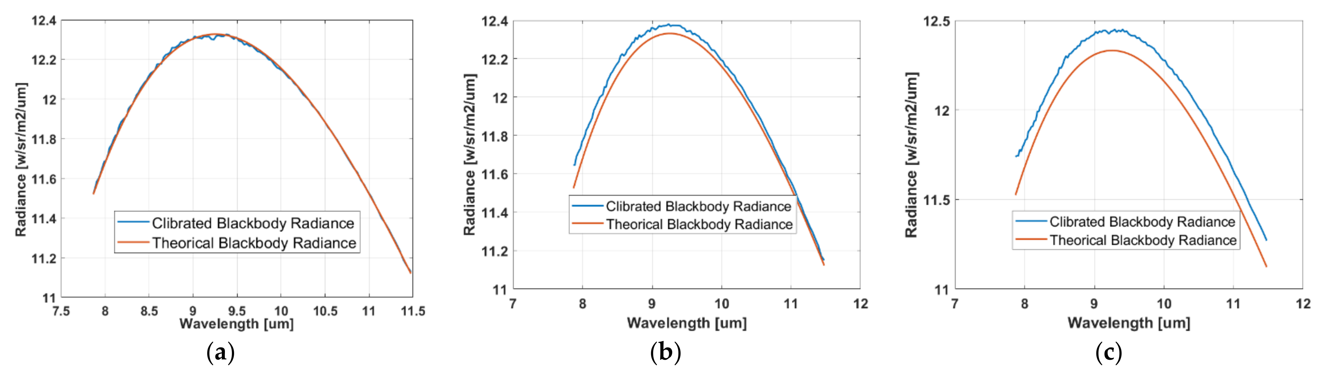
The goals of radiometric calibration are to convert the DN values into calibrated spectra in radiance units and to remove the interference of the internal self-emission of the instrument. However, because of the electric heating and ambient change, the sensor’s internal temperature can continue to rise with the increase of the instrument’s running time, leading to calculation errors due to the instrument’s self-emission. In order to quantitatively estimate the calibration performance of the Hyper-Cam LW sensor, the calibrated radiance spectra of a blackbody object and the theoretical spectra calculated using Planck’s function were compared and their calibration errors were recorded at various internal temperature differences (TDs), as shown in Figure 3.
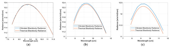
Figure 3.
Radiometric calibration error at various sensor internal temperature differences (TDs): (a) TD = 0.1 K; (b) TD = 0.9 K; (c) TD = 2.2 K.
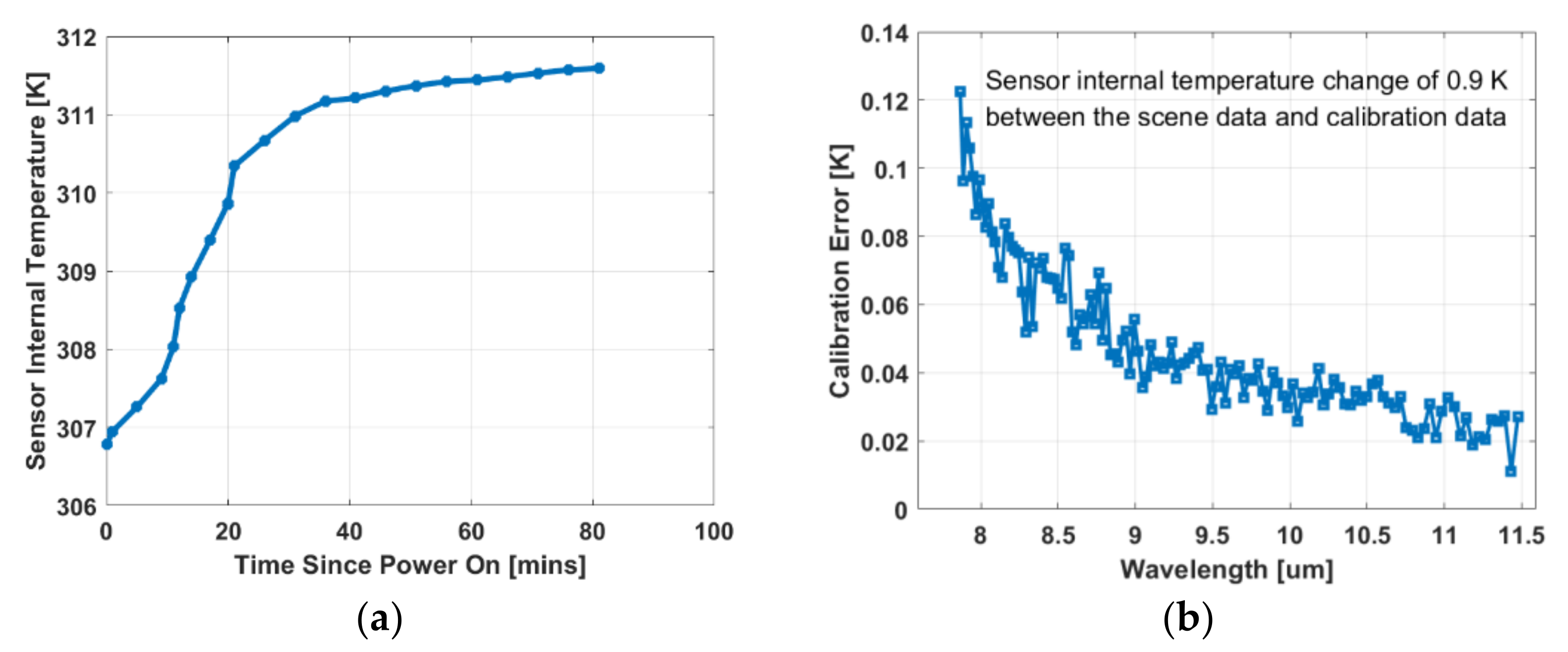
Figure 3 shows that the calibration error increased as the TD value increased. Generally speaking, a temperature inversion accuracy of 1 K requires the calibration error to be controlled within 0.5 K. Therefore, the TD should be kept within a small range. Figure 4a shows the temperature change trend of the Hyper-Cam LW instrument. This shows that the sensor’s internal temperature sharply increased as the power-on time became longer and gradually stabilized after approximately 40 min. Figure 4b shows that when the TD value was 0.9 K, the calibration error of each band was within 0.5 K. In addition, since the field environment was relatively unstable compared to the indoor environment, the instrument may have taken a longer time to reach a stable state. This depended on the specific measurement conditions.
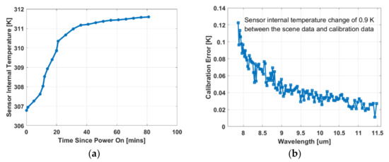
Figure 4.
Instrument calibration performance test: (a) sensor internal temperature change with time; (b) the calibration error in brightness temperature units when the TD equaled 0.9 K.
All these findings indicate that, in order to ensure the quality of Hyper-Cam LW radiation calibration, the recommended measurement time is a period after at least 40 min from power on, which will keep the radiation error of the sensor within 0.5 K.
2.2.2. Measurement Noise Level Estimation
The noise level of the Hyper-Cam LW sensor was evaluated using the noise-equivalent spectral radiance (NESR) indicator. According to the imaging principles of the Hyper-Cam LW sensor, the theoretical calculation of the NESR can be expressed as shown in the following equation:
where is the spectral resolution, is the optical solid angle, is the transmittance of the optical system, is the instrument detection rate, is the photosensitive surface area, and is the integral time of the measurement configuration.
The NESR is related to the spectral resolution and the integral time for the Hyper-Cam LW sensor with a specific optical system, according to Equation (2). In the noise level estimation, the NESR was calculated as the pixel-wise standard deviation of the radiance over multiple successive data cubes from the same target. The band-averaged noise-equivalent delta temperature (NEDT) was also calculated for every band based on the NESR. The statistical noise distribution of the NESR and NEDT is shown in Figure 5.
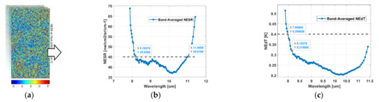
Figure 5.
Noise level estimation: (a) visualization of the single-band NESR values at 10 µm; (b) the band-averaged NESR; (c) the band-averaged NEDT.
It is apparent that the measured data acquired using the Hyper-Cam LW sensor contained a lot of noise. It is also apparent that the NEDT value of each band was larger than 0.2 K over the whole spectral range, which indicates that the Hyper-Cam sensor had very high measurement noise compared to the non-imaging instruments (at around 0.01 K through most of the TIR bands) [17]. All of these findings illustrate that preprocessing methods must be adopted to improve the quality of field-acquired data when using the Hyper-Cam LW sensor.
2.3. Field Data Acquisition
2.3.1. Instrument and Sample Preparation
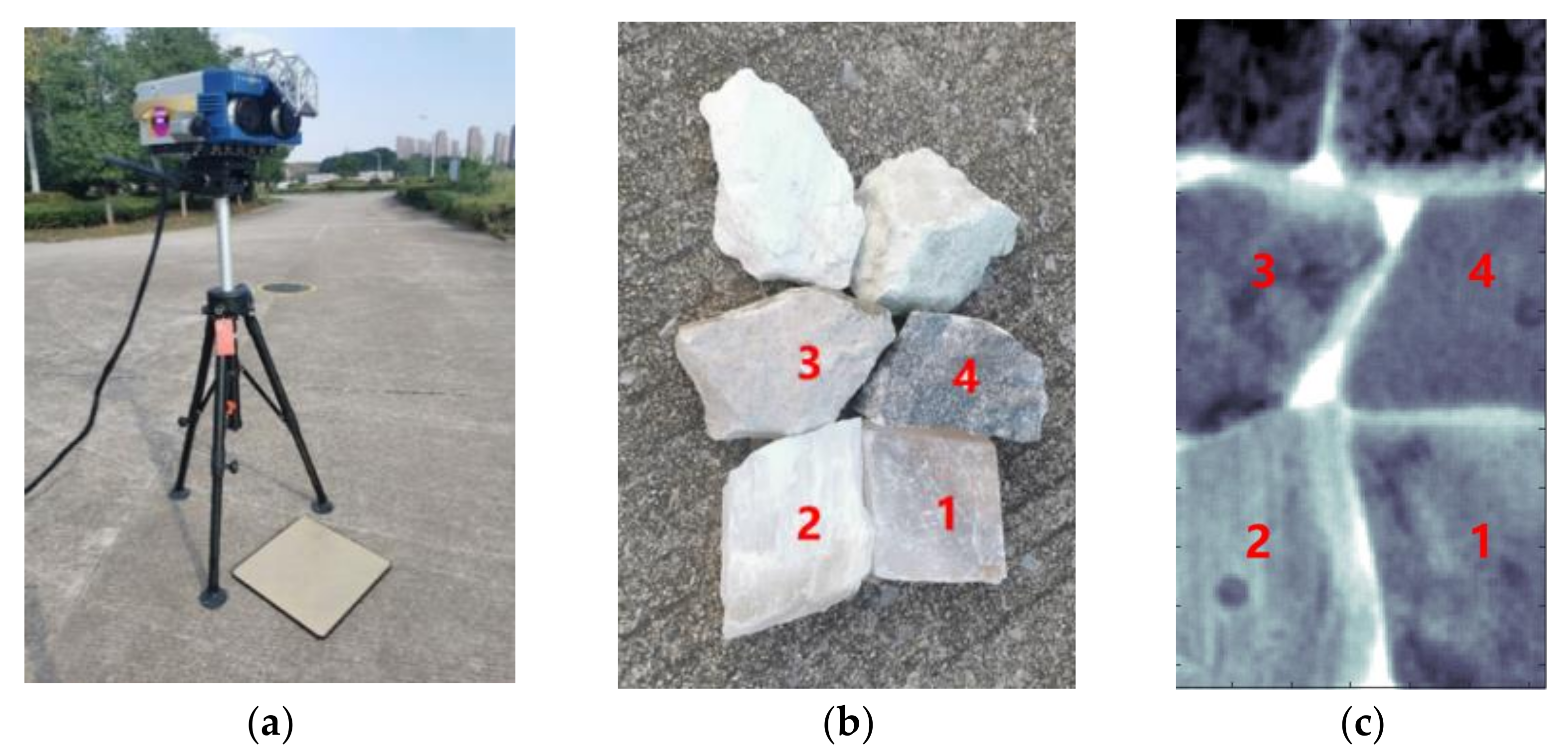
The instrument setup and mineral samples are shown in Figure 6. The Hyper-Cam sensor was mounted on a tripod and a modified optical lens was used for the vertical measurements to maintain consistency with the observation geometry of the Model 102F spectrometer. The instrument operations were performed until the detector temperature of the sensor stabilized at around 80 K.

Figure 6.
Field-based TIR hyperspectral imagery measurement scene and samples: (a) the field measurement scene and the Hyper-Cam LW sensor; (b) the used mineral samples; (c) the corresponding TIR imagery.
The mineral samples used in this study were calcite (No. 1), fibrous gypsum (No. 2), dolomite (No. 3), and anhydrite (No. 4). The size of all the samples was around 6 × 9 . All these materials have distinct emissivity signatures, which facilitated the evaluation of the processing results. Attention must be paid to avoiding rapid temperature changes of samples, so they were exposed to the experimental scene for some time in order to reach thermal equilibrium between the samples and the field environment.
2.3.2. Imagery Calibration and Measurement
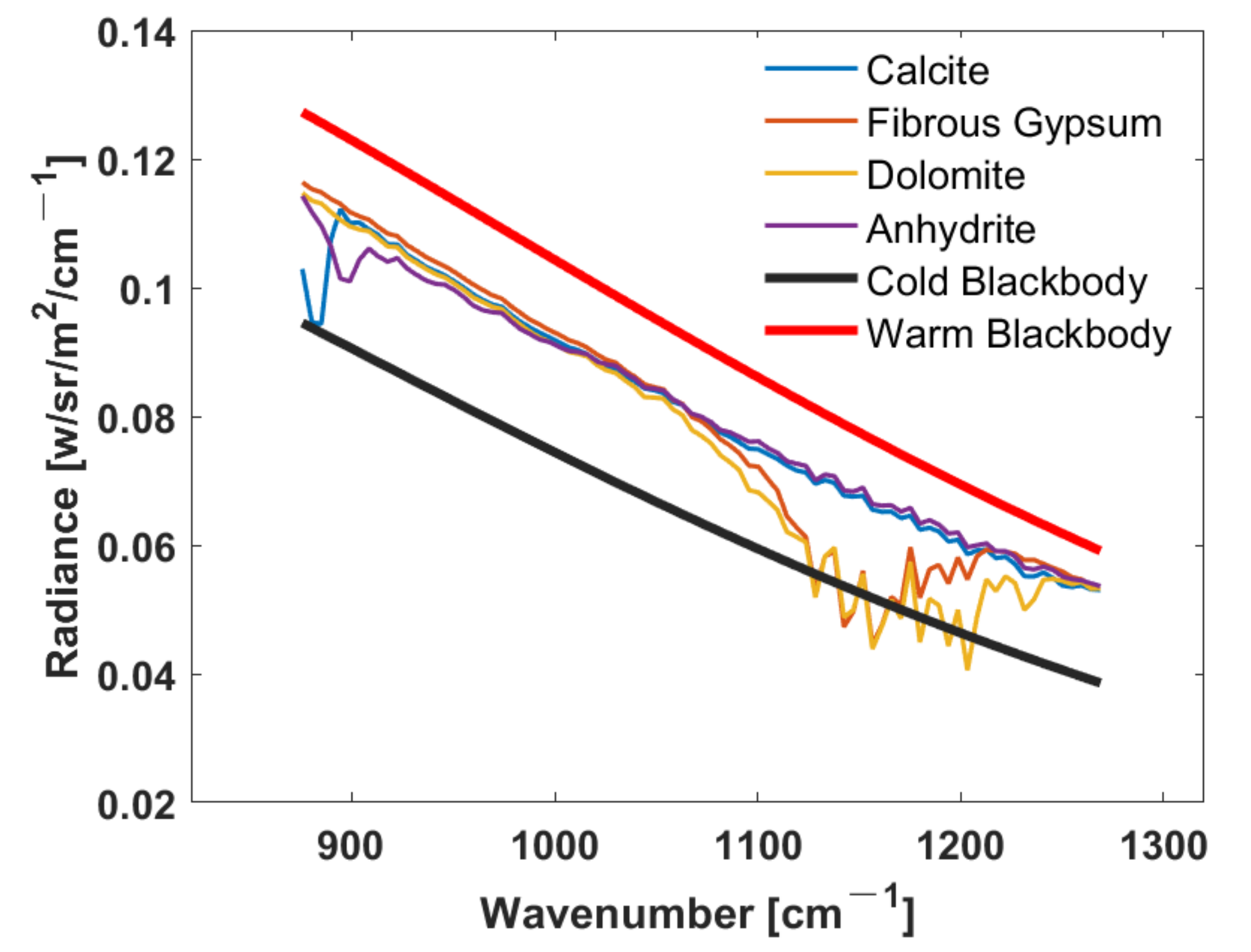
Before the measurement of the targets, the two blackbodies were measured for the radiometric calibration, and their temperature stability was found to be less than 0.03 K. It should be noted that the radiance spectra of the cold and warm blackbodies should frame all the radiance spectra emitted from a scene (Figure 7) to avoid the nonlinearity of instrument response. At the same time, it is recommended that the cold blackbody temperature should be just below ambient temperature and the warm blackbody temperature should be just above the warmest sample temperature. Since the temperatures of two internal blackbodies can be adjusted manually, the temperatures of cold and warm blackbodies should be set to around the values of corresponding temperatures of the coldest and warmest targets. In this study, the temperatures of the cold and warm blackbodies were set to 10 and 30 °C, respectively. Attention should also be paid to ensuring that the acquisition duration of a TIR HSI should be as short as possible in order to guarantee environmental consistency and exclude sample temperature variation during the measurement time. Here, the data acquisition was conducted at 40 min after powering on the instrument. Limited by the focal length of the instrument, the distance between the measured samples and the sensor was 1.7 m in this study.

Figure 7.
The radiance spectra of both the samples and the two calibration blackbodies.
2.3.3. Environmental Radiation Measurement
The radiance reaching the sensor for field-based measurements includes both the target radiance and environmental radiance. Generally speaking, the environmental radiance reflected from the target surface comes from both the atmosphere and the surrounding solid objects, e.g., trees and buildings. In this study, the environmental radiance was measured immediately after the sample measurement via the measurement of a diffuse and reflective plate—a gold-coated panel—whose directional hemispherical emissivity value was 0.95. The panel temperature was recorded by a contact thermometer: the Fluke 54-IIB contact thermometer. It should also be noted that the location, orientation, and bidirectional reflectance distribution function of the reflective panel should be identical to those of the measured objects.
3. Data Preprocessing and Quality Improvement
In this section, the noise, atmospheric influence, and environmental radiance are discussed and preliminary corresponding solutions are proposed. Firstly, the field measurements of a TIR imaging spectrometer contain more severe noise than the measurements of a non-imaging spectrometer. Secondly, previous studies [23,24] have explicitly pointed out that the distance between the samples and sensor should be less than 1 m in order to minimize the effects of the atmosphere. However, the shortest focus length of the Hyper-Cam LW sensor is 1.7 m, so the influence of atmospheric transmittance and upwelling radiance should be taken into consideration. The environmental radiance should be corrected for the radiation from the gold panel. Finally, band selection should also be carried out to remove the problem bands from the whole image data cube, which can negatively impact the retrieval results.
3.1. TIR Hyperspectral Imagery Denoising
As noted in the quantitative analysis in Section 2.2.2, the NEDT magnitude is larger than 0.2 K over the spectral range. This undesirable noise could generate serious deviation of the quantitative inversion. It is therefore necessary to remove or minimize measurement noise through appropriate denoising methods in order to promote more accurate spectral emissivity retrieval. With the increase of the spectral bands for the Hyper-Cam LW instrument with a spectral resolution of 6 cm−1, the atmospheric spectra also become rough, and spectral denoising methods can destroy atmospheric information while removing noise. Therefore, spatial denoising is a better choice for the TIR hyperspectral imagery of the Hyper-Cam LW instrument with numerous narrow bands. In this study, in order to select an appropriate denoising method, the noise type and distribution were first investigated using a blackbody object whose emissivity was known, as shown in Figure 8.

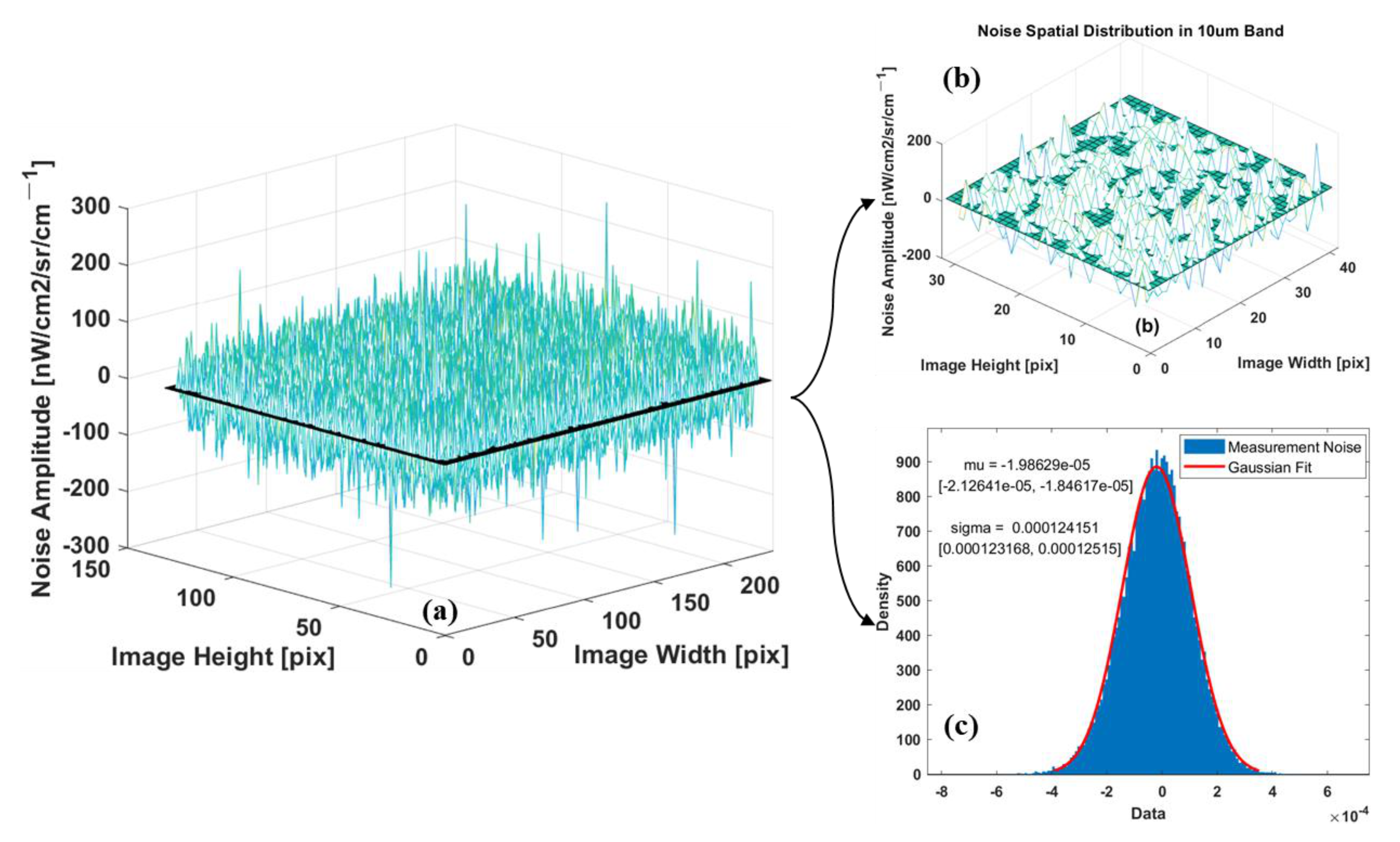
Figure 8.
TIR hyperspectral imagery noise analysis: (a) the pixel-wise noise in the 10 µm band; (b) the noise for a small random window; (c) the magnitude distribution of all the pixels in the 10 µm band.
From Figure 8c, it is clear that Gaussian function could well-fit the noise histogram with the parameters of mean and standard deviation in the 95% confidence interval (mu represents mean and sigma represents standard deviation). The noise type in both the whole image and a random window approximates the Gaussian distribution. Therefore, a Gaussian convolution method [43] was adopted for the spatial denoising to improve the noise quality of each band. In this method, considering that the noise type of a small window also approximates Gaussian distribution, a weighting template is calculated using the Gaussian kernel model, and then the weighting template is convolved with the whole TIR hyperspectral image using a moving window, which can be written as:
where represent the pixel location in the imagery; are the width and length of the template window; and is the calculated weighting matrix.
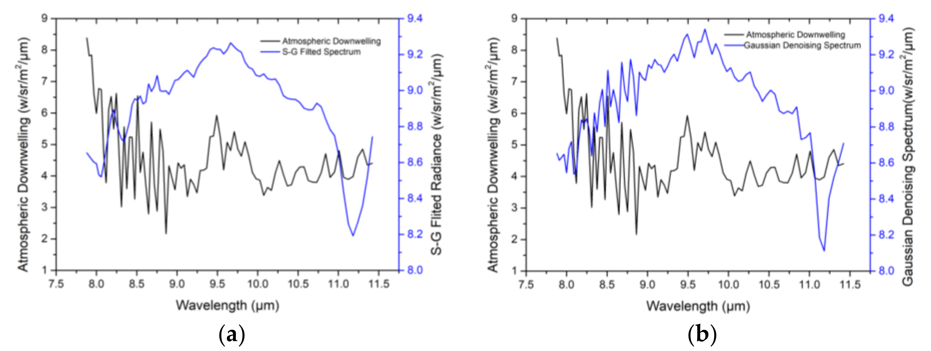
The window size of the Gaussian template is 3 × 3 pixels. This denoising method can eliminate the noise in experimental imagery while maintaining the atmospheric features contained in the collected data. Regarding the imagery acquired by the Hyper-Cam LW instrument, the cost of the spatial ambiguity can be neglected because the spatial resolution reaches up to 0.5 mm when the measurement distance is 1.7 m. To illustrate the difference between spectral and spatial denoising, a comparison between the Savitzky–Golay (S–G) spectral filter [44] and Gaussian spatial denoising is provided in Figure 9.
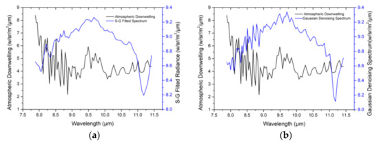
Figure 9.
Comparison between spectral and spatial denoising for Hyper-Cam LW hyperspectral imagery: (a) comparison between S–G-filtered image radiance and atmospheric downwelling; (b) comparison between Gaussian spatial denoising result and atmospheric downwelling.
It is clear from Figure 9a that the S–G-filtered image spectrum was relatively smooth and did not retain the characteristics of downward atmospheric radiation measured with a gold-plated plate. In contrast, the Gaussian spatial denoising image spectrum preserved the features of atmospheric downwelling. In addition, since the following TES methods utilize the relationship between ground-emitted radiance and atmospheric downwelling radiance, the changes of atmospheric downwelling radiance will interfere with the performance of TES methods. Therefore, atmospheric features should be preserved as much as possible during denoising. A spectral filter removes the atmospheric downwelling information contained in the measured radiance spectrum. In contrast, the spatial convolution denoising maintains these features of the atmospheric radiance in the spectral dimension.
3.2. Environmental Radiance Correction and Atmospheric Effect Analysis
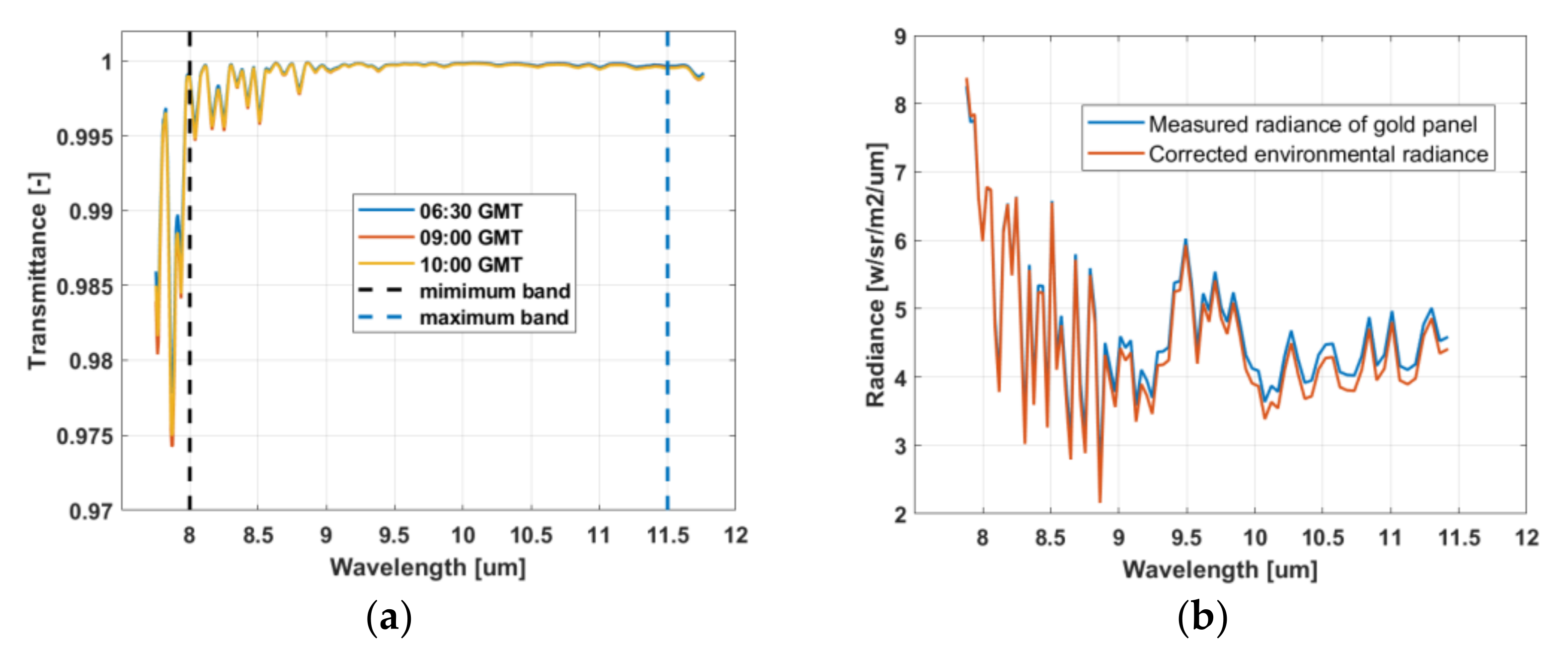
Previous studies have pointed out that the atmospheric effect between samples and sensor should be considered if the distance is more than 1 m. Since the minimum focus distance of the Hyper-Cam sensor is 1.7 m, the effects of atmospheric transmittance and upwelling radiance should be analyzed for field-based measurements. In our work, atmospheric simulation was conducted using MODTRAN®5.2 with the meteorological data of three periods during the time of the field-based measurements, as shown in Figure 10a. The imaging spectral range of the Hyper-Cam LW sensor lies between the two black dotted lines, and the transmittance value of each band was greater than 0.995, indicating that these factors could also be ignored for our field-based measurement conditions.
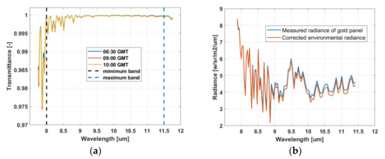
Figure 10.
(a) Simulated atmospheric transmittance by MODTRAN®5.2; (b) comparison between the corrected environmental radiance and the measured radiance of the gold-coated panel.
In addition, the environmental radiance could be corrected based on the imagery radiance of the gold-coated panel that was measured immediately after the sample measurements, according to Equation (4). As shown in Figure 10b, a comparison between the corrected environmental radiance and the measured radiance of the gold-coated panel was conducted. The difference between these two radiance spectra demonstrates the need for gold panel radiance correction.
where is the environmental radiance, is the image radiance of the gold panel, is the panel emissivity, and is the Planck radiance at panel temperature .
3.3. Band Selection
There were 85 bands in total for the final collected hyperspectral imagery. However, the factors of radiometric calibration error and measurement noise could have degraded the data quality in some bands. In practice, the magnitude of the measurement noise in the different bands showed a large variation for the experimental data, as shown in Section 2.2.2, Figure 5. The NEDT values of all the bands were larger than 0.2 K, which illustrates that the Hyper-Cam LW sensor has very high measurement noise compared to a non-imaging instrument (at around 0.01 K) through most of the TIR bands [22]. In addition, it is apparent that the measurement noise magnitude sharply increased with the decrease of the wavelength before 8.18 µm, and the NEDT values of the bands before 8 µm were higher than 0.4 K. Bands with large high-frequency noise can alter spectrum roughness and affect the smoothness-based TES algorithms [30]. Thus, the bands with heavy noise below 8 µm were removed, and the remaining bands were selected for the data improvement and spectral emissivity retrieval.
4. Temperature and Emissivity Separation Algorithms
4.1. Thermal Infrared Radiative Transfer Model for Field Measurement
The radiance emitted by an object propagates through the atmosphere and is recorded by a TIR sensor in three main parts—ground sample emission radiance, atmospheric radiance, and environmental radiance—which can be formulated as the radiative transfer equation (RTE):
where is the total radiance reaching the sensor, is the central wavelength of each channel, is the emissivity, and and are the atmospheric transmittance and upwelling radiance, respectively. It should be noted that the environmental radiance is composed of the atmospheric downwelling radiance and the background radiance emitted by trees, buildings, clouds, etc.
4.2. The Temperature and Emissivity Separation Methods for Emissivity Retrieval
In this section, we describe three types of widely used TES algorithms, i.e., ISSTES, FLAASH-IR, and the modified ASTER-TES algorithm, and we extend an empirically constrained method for the Hyper-Cam LW imagery that was originally designed for multispectral TIR imagery with six bands.
4.2.1. The ISSTES Method
The ISSTES method is a physically constrained method designed by Borel [45] that exploits the fact that the emissivity spectrum of a solid object is smoother than the atmospheric features. The ISSTES algorithm involves defining a family of emissivity curves indexed by the surface temperature by rearranging Equation (5) as follows:
According to Equation (6), given a land surface temperature (LST) estimation, the corresponding emissivity spectrum can be calculated if the atmospheric parameters are known. Then, if the smoothness criterion of the emissivity curve is determined, the smoothness of a series of emissivity curves can be calculated with regard to the different temperatures around the true surface temperature, and the estimated emissivity spectrum corresponds to the temperature that leads to the smoothest result. The smoothness criterion used in ISSTES was designed as follows:
where S is the calculated smoothness criterion value and N is the band number of the hyperspectral data.
4.2.2. The FLAASH-IR Method
FLAASH-IR is an integrated method, which includes both atmospheric correction and TES for TIR hyperspectral imagery [46], that has previously been investigated with Hyper-Cam LW ground and airborne data to extract surface emissivity information [40,44].
In FLAASH-IR, the atmospheric correction parameter can be automatically retrieved based on the atmospheric parameter lookup table generated by MODTRAN. After obtaining the atmospheric parameters, a smoothness-based TES was used to separate temperature and emissivity from the ground-leaving radiance. In addition, instead of the emissivity smoothness index utilized in ISSTES, FLAASH-IR calculates the corresponding sensor output radiance according to the RTE, and the smoothness index uses the standard deviation σ of the calculated radiance and the real sensor output radiance. The principle is shown in Equation (8) as follows:
4.2.3. The Modified ASTER-TES Method
The ASTER-TES method is an empirically constrained method that was originally designed for TIR multispectral data. This method includes three modules: (1) the normalized emissivity method (NEM) module, (2) the ratio (RAT) module, and (3) the maximum-minimum relative emissivity difference (MMD) module. The technical route of the ASTER-TES method is detailed in [8]. The ASTER-TES method has been modified and applied to different sensors with more than four bands in the TIR region. However, to the best of our knowledge, to date, no researchers have attempted to migrate the algorithm to Hyper-Cam LW data. In this paper, a modified ASTER-TES method, as an expansion of ASTER-TES, is proposed for use with Hyper-Cam LW data.
The empirical relationship between the minimum emissivity value and the MMD is the key feature of the method, and it needs to be established for specific sensor data. In this study, to obtain a reliable empirical relationship, 198 spectra extracted from the JHU spectral library (including water, vegetation, soil, and rock spectra, which were converted to emissivity using Kirchhoff’s Law and resampled according to the spectral information of the Hyper-Cam LW data) were used to fit the relationship. The fitting results of the empirical relationship for the Hyper-Cam LW sensor are shown in Figure 11. It is clear that the parameters of the empirical relationship between the minimum emissivity value and the MMD for Hyper-Cam LW data were distinctly different from those for other TIR sensors, such as ASTER and TASI.
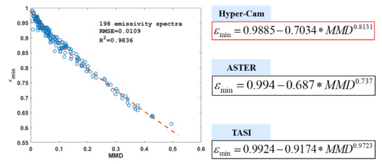
Figure 11.
The fitting results for the relationship between the MMD and the minimum emissivity for Hyper-Cam LW field data.
4.3. Evaluation Indicator
To mathematically evaluate the retrievals, three indicators of the root-mean-square error (RMSE), spectral angle (SA), and spectral residual (SR) were used in this research to evaluate the retrieved results from the different approaches. The calculations of these indicators are as follows:
where is the band value of retrieved emissivity spectrum, is the band value of reference emissivity spectrum, and N is the band number of the hyperspectral data.
5. Results and Discussion
The final temperature and emissivity information of the objects of interest were obtained through field data acquisition, data improvement, and TES processing. In this section, the retrieved temperature and emissivity maps are displayed to demonstrate the advantages of the TIR imaging spectrometer in reflecting the spatial variation over the sample surface. In addition, a qualitative analysis and comparison between the results of the three different methods are provided. Finally, to illustrate the retrieval accuracy of the proposed solution, this section presents a quantitative assessment that was carried out in the spectral dimension.
5.1. Qualitative Evaluation of the Temperature and Emissivity Maps
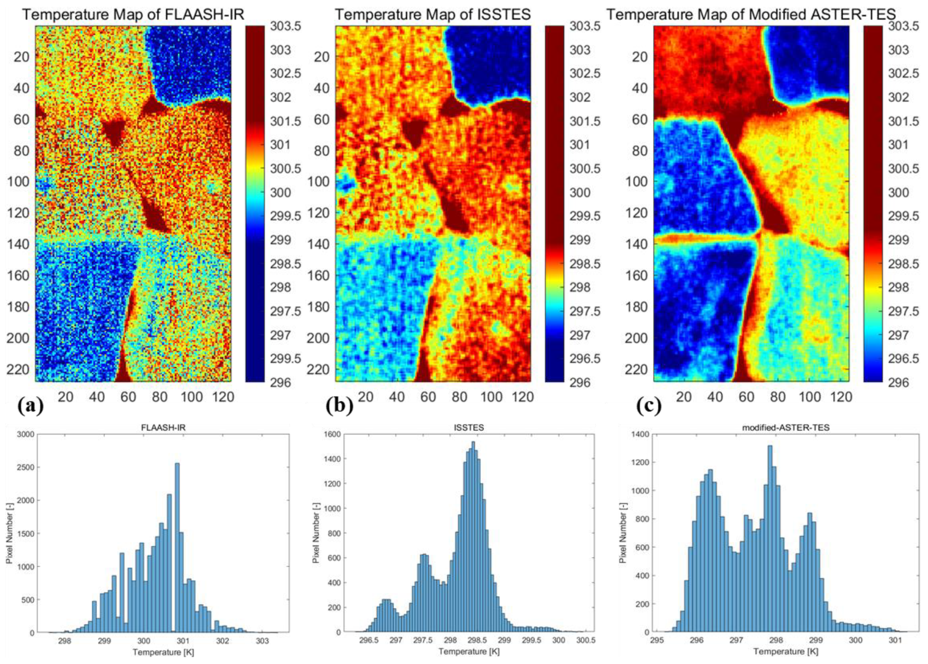
Compared to a non-imaging TIR spectrometer, the retrieved temperature and emissivity maps contained fine spatial information that could reflect the material distribution of the sample surface. Figure 12 shows the final temperature maps and temperature histograms for the three approaches investigated in this paper. It can be seen that all the temperature maps reflect the spatial temperature distribution of each sample. The temperature map of FLAASH-IR shows serious noise pollution, which results in the image granularity phenomenon of impulse noise, while this phenomenon does not appear in the maps of the two other methods. The texture and tone are also clean and uniform, which demonstrates that the spatial convolution denoising had a remarkably positive effect. In addition, temperature histograms of the three retrieval methods were generated to illustrate the temperature distribution of each method’s result, as shown in Figure 12. It is clear that the histograms of ISSTES and ASTER-TES have three peaks, which represent the TDs of the different samples, while the histogram of FLAASH-IR has only one peak. The temperature distribution of the ISSTES method also shows the best continuity. This shows that the temperature distribution consistency of the ISSTES and modified ASTER-TES is better than that of the FLAASH-IR temperature map.
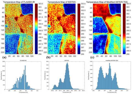
Figure 12.
Retrieved temperature maps and corresponding temperature histograms: (a) FLAASH-IR, (b) ISSTES, and (c) modified ASTER-TES.
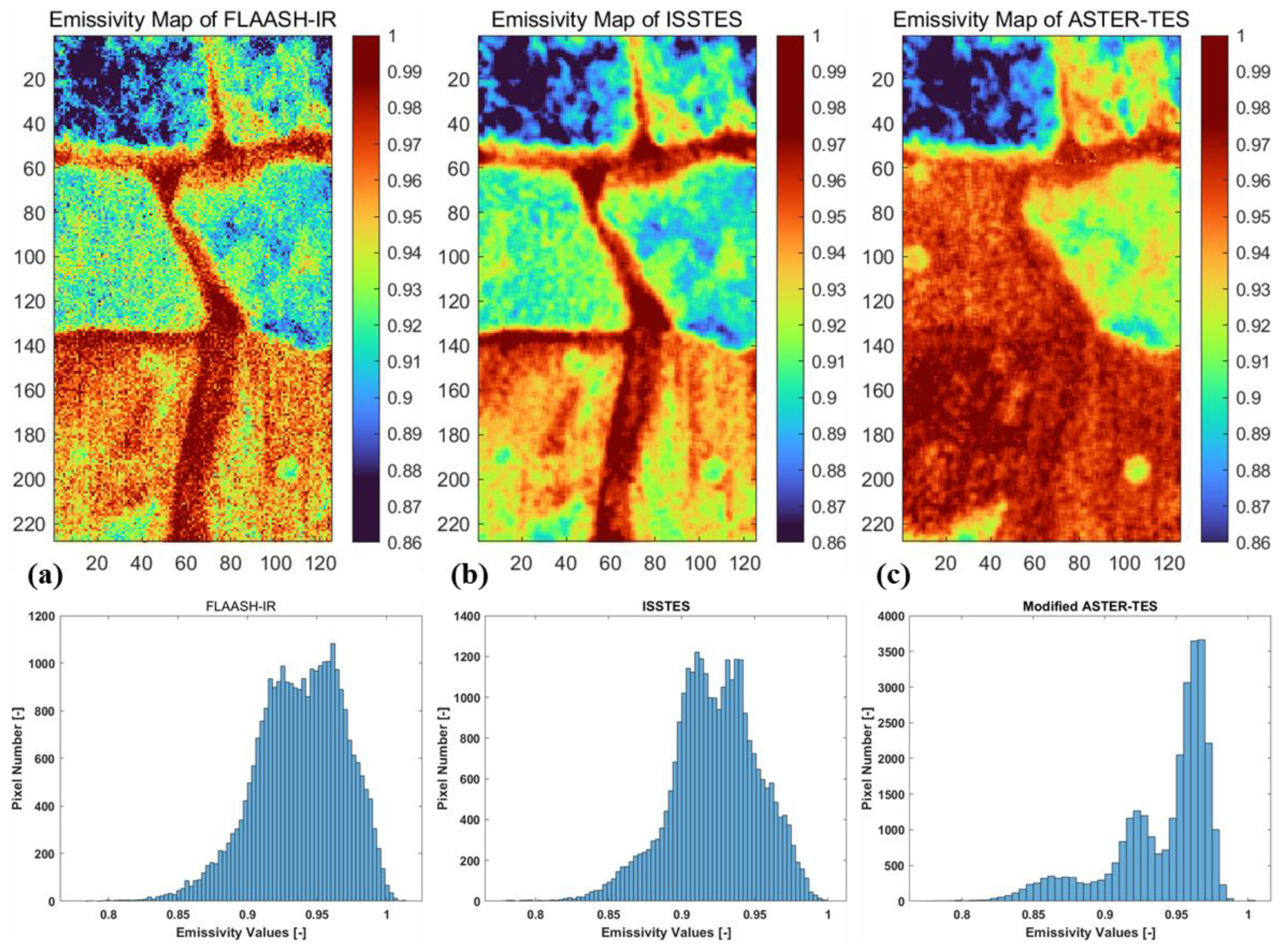
The recorded temperature range of the measurement scene obtained using a contact thermometer was between 296.5 and 299.2 K, which was closest to the result of ISSTES. FLAASH-IR tended to overestimate the temperature by around 2 K, and the temperature range of FLAASH-IR was between 297.6 and 303.3 K. The temperature range of the ISSTES and modified ASTER-TES methods represents a relatively reasonable range for the Hyper-Cam LW sensor. In addition, the same phenomenon can be seen in the retrieved emissivity maps. One band of the emissivity map at 10 µm is shown in Figure 13, where it is clear that the image granularity phenomenon of impulse noise also appears in the FLAASH-IR emissivity map and the discriminability of the different samples is poor for the modified ASTER-TES emissivity map, which may have been caused by the spectral emissivity similarity between the samples of calcite, fibrous gypsum, and anhydrite. That is, the ASTER-TES method was unable to highlight the subtle spectral difference among these three samples. In contrast, ISSTES showed the best definition and discriminability for these environmental samples.
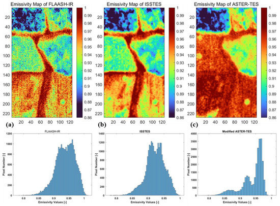
Figure 13.
Retrieved emissivity maps in the 10 µm band: (a) result of FLAASH-IR; (b) result of ISSTES; (c) result of the modified ASTER-TES method.
5.2. Quantitative Accuracy Evaluation of the Retrieved Emissivity Spectra
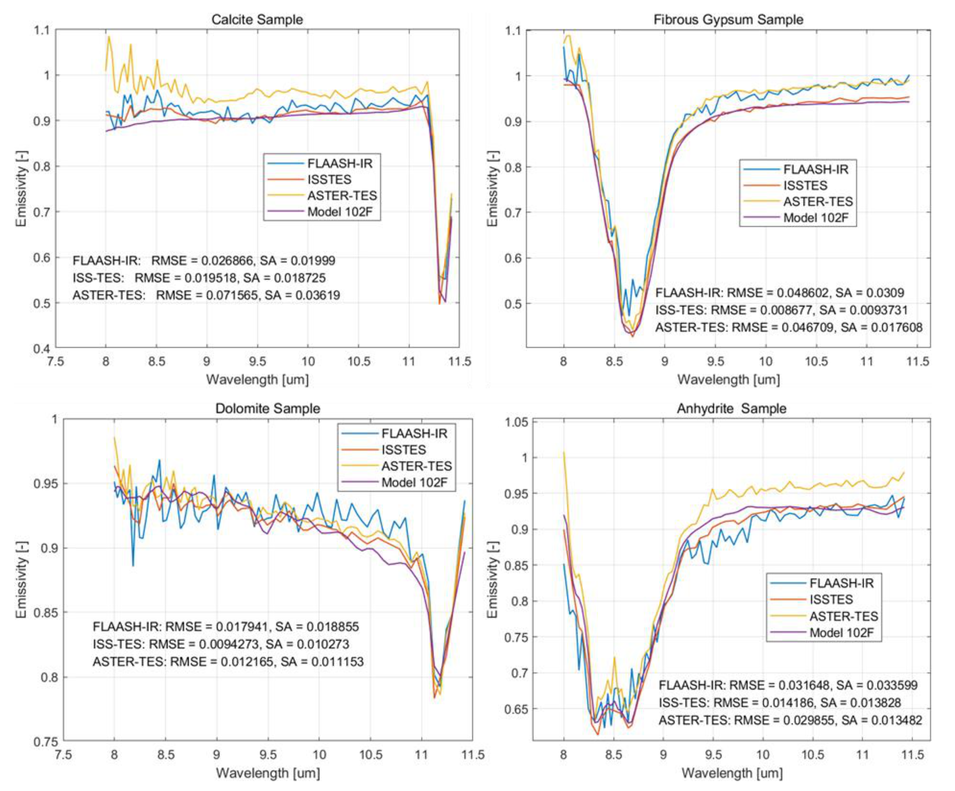
Four different mineral samples were chosen to validate the quality of the retrieved emissivity spectra, i.e., calcite, fibrous gypsum, dolomite, and anhydrite. Firstly, the retrieved emissivity spectra obtained with FLAASH-IR, ISSTES, and the modified ASTER-TES method were compared to the standard spectra. These standard spectra were measured using the widely used D&P Model 102F spectrometer, which is a non-imaging FT-TIR spectrometer. The three indicators were then calculated to quantitatively illustrate the inversion precision. The comparison is shown in Figure 14, with the RMSE and SA values listed in the corresponding figures.
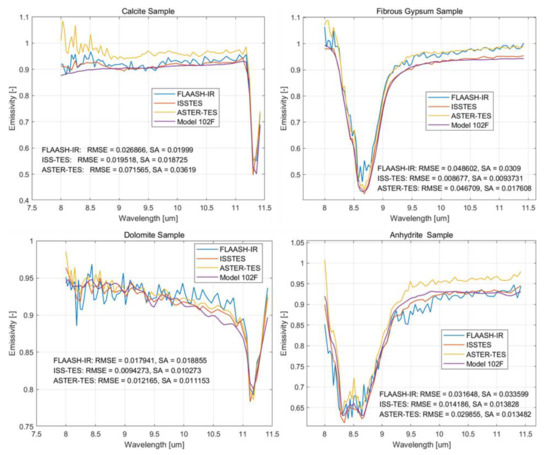
Figure 14.
Emissivity quantitative evaluation for the three different methods and a comparison with the reference emissivity spectra measured by the D&P Model 102F spectrometer.
In Figure 14, the RMSE and SA values are provided to quantitatively evaluate the retrieval accuracy of the emissivity spectra. The RMSE reflects the deviation between the retrieved emissivity and the standard spectra, and the SA reflects the spectral shape and trend consistency. It is clear that the final emissivity spectra retrieved by ISSTES had the smallest SA values for these experimental samples, with values of 0.0187, 0.0093, 0.010, and 0.0138 for calcite, fibrous gypsum, dolomite, and anhydrite, respectively. The results of ISSTES also had the smallest RMSE values. In addition, ISSTES could obtain a smoother LSE than the other methods, which was consistent with the emissivity characteristics of solid materials. All these findings indicate that the ISSTES method can be used to obtain high-quality emissivity spectra from field-measured data and is superior to the other two methods.
For FLAASH-IR, a distinct characteristic of the emissivity spectra is that they are relatively irregular compared to those from the other two processing methods. The FLAASH-IR emissivity values of some bands below 8.5 μm are greater than 1.0. This may be caused by measurement noise. For a true emissivity value close to 1.0, the retrieval emissivity result may be greater than 1.0. In addition, due to the empirical relationship in ASTER-TES, the relationship may also result in emissivity values greater than 1.0. For ISSTES, since the method is based on physical retrieval and the noise is eliminated via spatial convolution denoising, the result of emissivity value was less than 1. It should be noted that, compared to the spectral range with relatively high emissivity values, FLAASH-IR and ASTER-TES have coarser features in the spectral range with low emissivity values. This phenomenon is clearly shown in the anhydrite sample spectra shown in Figure 12, which suggests that these two methods may have retained the atmospheric residuals. Furthermore, an interesting phenomenon is that the magnitude of the calcite and fibrous gypsum emissivity spectra from FLAASH-IR was greater than that of the standard spectra, while the magnitude of the dolomite and anhydrite emissivity spectra was smaller than that of the standard spectra. One explanation for this phenomenon is that the radiance of the surrounding objects contained in the background was not considered in FLAASH-IR, leading to incorrect environmental radiance estimation.
The modified ASTER-TES method showed good performance in retrieving the emissivity spectra that had high spectral contrast. However, it tended to overestimate the emissivity values for all the samples used in this study. This was mainly because the maximum emissivity values of mineral materials are normally lower than those of natural materials, leading to the fitting coefficients not being well-represented for these mineral materials. In addition, it is inconvenient to migrate the original ASTER-TES method to the Hyper-Cam LW sensor because the spectral resolution of the Hyper-Cam LW sensor is adjustable and the data may have different spectral parameters for different measurements.
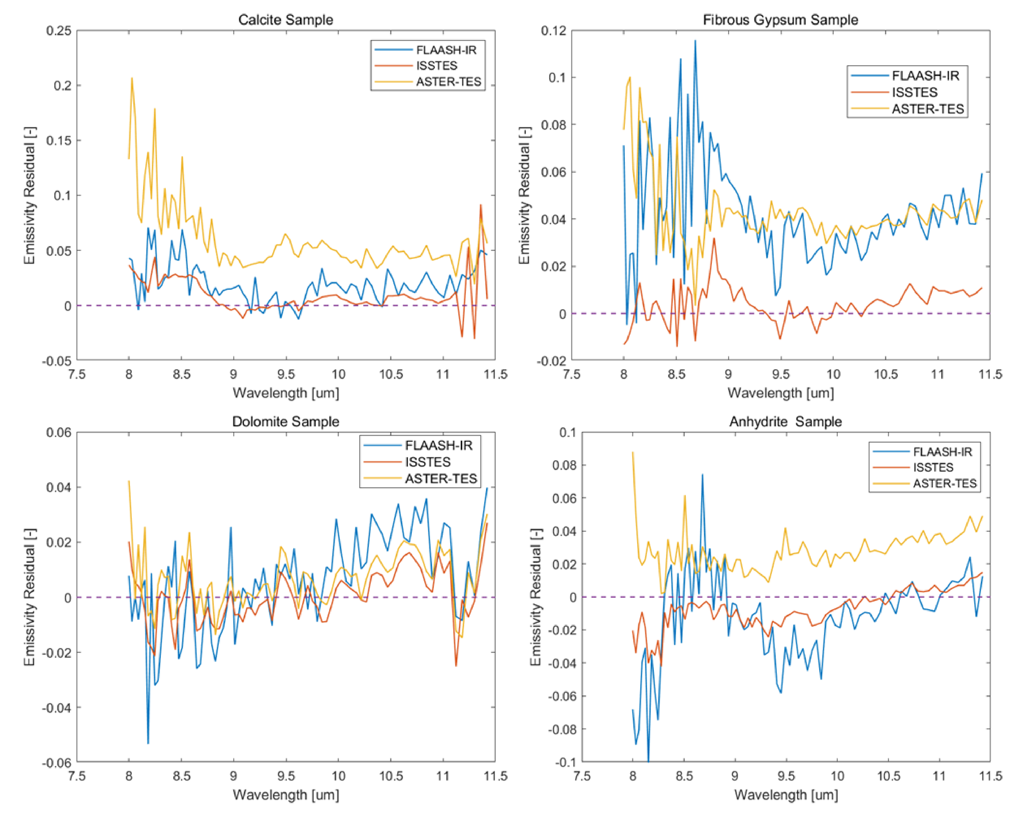
The SRs of the three methods were calculated and are shown in Figure 15. From this comparison, it can be seen that the emissivity spectra of the ISSTES method showed the best agreement with the standard spectra in both shape and magnitude. However, there were certain magnitude differences between the ISSTES results and the reference spectra for the calcite, dolomite, and anhydrite samples. These discrepancies were mainly introduced by the different spatial resolutions. However, the spectral resolution difference of the measurement configurations may also have had an influence. Overall, it can be seen that, through the use of the proposed data acquisition and ISSTES processing method, high-quality emissivity spectra can be obtained using the Hyper-Cam LW FT-TIR hyperspectral imager, which can reach the measurement accuracy of the Model 102F spectrometer.
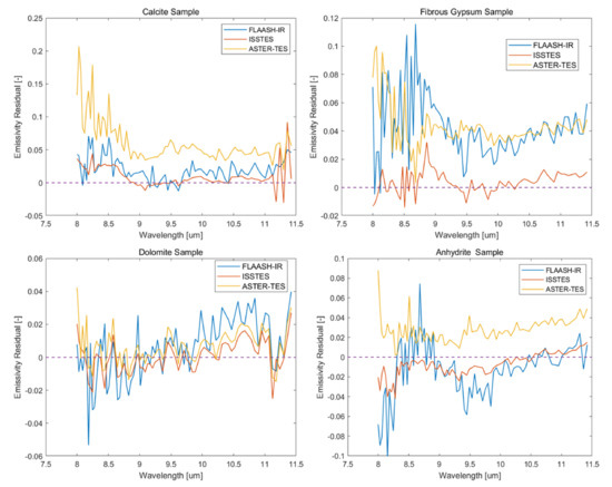
Figure 15.
The SRs of the retrieved emissivity of FLAASH-IR, ISSTES, and modified ASTER-TES and the standard emissivity spectra measured by a Model 102F spectrometer.
6. Conclusions
As an important physical quantity, emissivity spectra reflect material components and play a significant role in remote sensing. The current mainstream non-imaging spectrometers for single-point measurement neglect the spatial information of a scene. In contrast, TIR hyperspectral imagery has the advantages of high spectral and spatial resolutions, thus providing us with an opportunity to obtain fine ground imagery with emissivity spectral information. However, there are no recognized spectral emissivity measurement standards for a TIR hyperspectral imager in the field. In this study, the Hyper-Cam LW imaging spectrometer was utilized for field data acquisition. In addition, a processing chain including data acquisition, improvement, and emissivity retrieval algorithms was developed to obtain high-quality emissivity spectra.
The instrument performance of the Hyper-Cam LW sensor was tested, and the analysis demonstrated that measurements should be conducted after waiting at least 40 min from power on in order to avoid the rapid change of instrument temperature. The Hyper-Cam LW sensor also has very high measurement noise compared to the non-imaging instruments (at around 0.01 K) through most of the TIR bands. Preprocessing, including band selection and spatial denoising, was performed to improve the image quality for the spectral emissivity retrieval. It was found that the spatial denoising method is more effective than spectral dimension denoising because spatial dimension denoising does not damage the atmospheric characteristics. In this work, three widely used TES algorithms, ISSTES, modified ASTER-TES, and FLAASH-IR, were applied and compared for the retrieval of the sample emissivity. Compared to the other two algorithms, the ISSTES algorithm showed the best performance on the Hyper-Cam LW data according to the results distribution of temperature and emissivity images and the quantitative analysis of the RMSE, SA, and SR metrics. The ISSTES algorithm was found to be able to reach the precision of the standard spectra measured by the D&P Model 102F spectrometer. Therefore, the solution proposed in this paper could serve as a reference for high-quality emissivity spectra collection using an FT-TIR imaging spectrometer in the field. It should be stated that the proposed framework for the Hyper-Cam LW sensor is not an official package endowed with the instrument; it just proved to be a practical data acquisition and processing flow. Therefore, more advanced methods in each module could be used by specific scientific communities.
Based on the current research and processing models, applications of the Hyper-Cam LW sensor are still in the early stages. In this work, we mainly focused on the validation of instrument performance and emissivity retrieval methods using minerals. For the emissivity retrieval of both manmade and nature materials from the airborne platform, large measurement noise and atmospheric effects greatly attenuate the spectral characteristics. Therefore, more advanced denoising algorithms and atmospheric compensation methods should be elaborately studied. In our future work, an airborne campaign is planned to acquire airborne TIR hyperspectral imagery in order to validate the feasibility of retrieving LSE information from an aircraft platform.
Author Contributions
Conceptualization: L.C. and Y.Z.; methodology: L.G.; software: L.G.; validation: Z.J. and L.C.; formal analysis: L.G.; investigation: L.G.; resources: L.C. and Y.Z.; data curation: L.G.; writing—original draft preparation: L.G.; writing—review and editing: L.C. and Y.Z.; visualization: L.G.; supervision: L.C. and Y.Z.; project administration: L.C. and Y.Z.; funding acquisition: L.C. and Y.Z. All authors have read and agreed to the published version of the manuscript.
Funding
This research was supported by National Key Research and Development Program of China under Grant No.2020YFC1522703 and National Natural Science Foundation of China under Grant No.41771385 and 41622107.
Data Availability Statement
The data presented in this study are not available.
Acknowledgments
We gratefully acknowledge Wu Hua for his support and assistance during field data acquisition work and providing standard spectra, and we would like to thank the anonymous reviewers for their insightful advice.
Conflicts of Interest
The authors declare no conflict of interest.
References
- Manolakis, D.; Pieper, M.; Truslow, E.; Lockwood, R.; Weisner, A.; Jacobson, J.; Cooley, T. Longwave infrared hyperspectral imaging: Principles, progress, and challenges. IEEE Geosci. Remote Sens. Mag. 2019, 7, 72–100. [Google Scholar] [CrossRef]
- Li, Z.-L.; Wu, H.; Wang, N.; Qiu, S.; Sobrino, J.A.; Wan, Z.; Tang, B.-H.; Yan, G. Land surface emissivity retrieval from satellite data. Int. J. Remote Sens. 2013, 34, 3084–3127. [Google Scholar] [CrossRef]
- Ni, L.; Xu, H.G.; Zhou, X.M. Mineral Identification and Mapping by Synthesis of Hyperspectral VNIR/SWIR and Multispectral TIR Remotely Sensed Data with Different Classifiers. IEEE J. Sel. Top. Appl. Earth Obs. Remote Sens. 2020, 13, 3155–3163. [Google Scholar] [CrossRef]
- Puckrin, E.; Turcotte, C.S.; Lahaie, P.; Dubé, D.; Farley, V.; Lagueux, P.; Marcotte, F.; Chamberland, M. Airborne infrared-hyperspectral mapping for detection of gaseous and solid targets. SPIE Def. Secur. Sens. 2010, 7665, 10. [Google Scholar]
- Zhu, X.; Cao, L.; Wang, S.; Gao, L.; Zhong, Y.J.R.S. Anomaly Detection in Airborne Fourier Transform Thermal Infrared Spectrometer Images Based on Emissivity and a Segmented Low-Rank Prior. Remote Sens. 2021, 13, 754. [Google Scholar] [CrossRef]
- Fassnacht, F.E.; Latifi, H.; Stereńczak, K.; Modzelewska, A.; Lefsky, M.; Waser, L.T.; Straub, C.; Ghosh, A. Review of studies on tree species classification from remotely sensed data. Remote Sens. Environ. 2016, 186, 64–87. [Google Scholar] [CrossRef]
- Liu, H.; Wu, K.; Xu, H.; Xu, Y.J.R.S. Lithology Classification Using TASI Thermal Infrared Hyperspectral Data with Convolutional Neural Networks. Remote Sens. 2021, 13, 3117. [Google Scholar] [CrossRef]
- Gillespie, A.; Rokugawa, S.; Matsunaga, T.; Cothern, J.S.; Hook, S.; Kahle, A.B. A temperature and emissivity separation algorithm for Advanced Spaceborne Thermal Emission and Reflection Radiometer (ASTER) images. IEEE Trans. Geosci. Remote Sens. 1998, 36, 1113–1126. [Google Scholar] [CrossRef]
- Grigsby, S.P.; Hulley, G.C.; Roberts, D.A.; Scheele, C.; Ustin, S.L.; Alsina, M.M. Improved surface temperature estimates with MASTER/AVIRIS sensor fusion. Remote Sens. Environ. 2015, 167, 53–63. [Google Scholar] [CrossRef] [Green Version]
- Malakar, N.K.; Hulley, G.C. A water vapor scaling model for improved land surface temperature and emissivity separation of MODIS thermal infrared data. Remote Sens. Environ. 2016, 182, 252–264. [Google Scholar] [CrossRef]
- Li, Z.-L.; Tang, B.-H.; Wu, H.; Ren, H.; Yan, G.; Wan, Z.; Trigo, I.F.; Sobrino, J.A. Satellite-derived land surface temperature: Current status and perspectives. Remote Sens. Environ. 2013, 131, 14–37. [Google Scholar] [CrossRef] [Green Version]
- Ye, X.; Ren, H.; Liang, Y.; Zhu, J.; Guo, J.; Nie, J.; Zeng, H.; Zhao, Y.; Qian, Y. Cross-calibration of Chinese Gaofen-5 thermal infrared images and its improvement on land surface temperature retrieval. Int. J. Appl. Earth Obs. Geoinf. 2021, 101, 102357. [Google Scholar] [CrossRef]
- Yang, J.; Duan, S.-B.; Zhang, X.; Wu, P.; Huang, C.; Leng, P.; Gao, M.J.R.S. Evaluation of Seven Atmospheric Profiles from Reanalysis and Satellite-Derived Products: Implication for Single-Channel Land Surface Temperature Retrieval. Remote Sens. 2020, 12, 791. [Google Scholar] [CrossRef] [Green Version]
- Wan, Z.; Li, Z.-L. A physics-based algorithm for retrieving land-surface emissivity and temperature from EOS/MODIS data. IEEE Trans. Geosci. Remote Sens. 1997, 35, 980–996. [Google Scholar]
- Zhao, E.; Gao, C.; Yao, Y. New land surface temperature retrieval algorithm for heavy aerosol loading during nighttime from Gaofen-5 satellite data. Opt. Express 2020, 28, 2583–2599. [Google Scholar] [CrossRef]
- Yuan, L.; He, Z.; Lv, G.; Wang, Y.; Li, C.; Wang, J. Optical design, laboratory test, and calibration of airborne long wave infrared imaging spectrometer. Opt. Express 2017, 25, 22440–22454. [Google Scholar] [CrossRef]
- Hackwell, J.A.; Warren, D.W.; Bongiovi, R.P.; Hansel, S.J.; Hayhurst, T.L.; Mabry, D.J.; Sivjee, M.G.; Skinner, J.W. LWIR/MWIR imaging hyperspectral sensor for airborne and ground-based remote sensing. In Proceedings of the Imaging Spectrometry II, Denver, CO, USA., 4–9 August 1996; pp. 102–107. [Google Scholar]
- Wang, H.; Xiao, Q.; Li, H.; Zhong, B. Temperature and emissivity separation algorithm for TASI airborne thermal hyperspectral data. In Proceedings of the 2011 International Conference on Electronics, Communications and Control (ICECC), Ningbo, China, 9–11 September 2011; pp. 1075–1078. [Google Scholar]
- Montembeault, Y.; Lagueux, P.; Farley, V.; Villemaire, A.; Gross, K.C. Hyper-Cam: Hyperspectral IR imaging applications in defence innovative research. In Proceedings of the 2010 2nd Workshop on Hyperspectral Image and Signal Processing: Evolution in Remote Sensing, Reykjavik, Iceland, 14–16 June 2010; pp. 1–4. [Google Scholar]
- Yang, H.; Lifu, Z.; Yingqian, G.; Hu, S.; Li, X.; Genzhong, Z.; Qingxi, T. Temperature and Emissivity Separation from Thermal Airborne Hyperspectral Imager (TASI) Data. Photogramm. Eng. Remote Sens. 2013, 79, 1099–1107. [Google Scholar] [CrossRef]
- Zhang, Y.Z.; Wu, H.; Jiang, X.G.; Jiang, Y.Z.; Liu, Z.X.; Nerry, F. Land Surface Temperature and Emissivity Retrieval from Field-Measured Hyperspectral Thermal Infrared Data Using Wavelet Transform. Remote Sens. 2017, 9, 454. [Google Scholar] [CrossRef] [Green Version]
- Korb, A.R.; Dybwad, P.; Wadsworth, W.; Salisbury, J.W. Portable Fourier transform infrared spectroradiometer for field measurements of radiance and emissivity. Appl. Opt. 1996, 35, 1679–1692. [Google Scholar] [CrossRef] [Green Version]
- Salvaggio, C.; Miller, C.J. Methodologies and protocols for the collection of midwave and longwave infrared emissivity spectra using a portable field spectrometer. In Proceedings of the Algorithms for Multispectral, Hyperspectral, and Ultraspectral Imagery VII, Orlando, FL, USA, 16–19 April 2001; pp. 539–548. [Google Scholar]
- Christoph, H.; Simon, H.; Mark, V.D.M.; Wim, B.; Harald, V.D.W.; Henk, W.; Frank, V.R.; Boudewijn, D.S.; Freek, V.D.M. Thermal infrared spectrometer for Earth science remote sensing applications-instrument modifications and measurement procedures. Sensors 2011, 11, 10981–10999. [Google Scholar]
- Schlerf, M.; Rock, G.; Lagueux, P.; Ronellenfitsch, F.; Gerhards, M.; Hoffmann, L.; Udelhoven, T. A hyperspectral thermal infrared imaging instrument for natural resources applications. Remote Sens. 2012, 4, 3995–4009. [Google Scholar] [CrossRef] [Green Version]
- Liu, C.; Xu, R.; Xie, F.; Jin, J.; Yuan, L.; Lv, G.; Wang, Y.; Li, C.; Wang, J. New Airborne Thermal-Infrared Hyperspectral Imager System: Initial Validation. IEEE J. Sel. Top. Appl. Earth Obs. Remote Sens. 2020, 13, 4149–4165. [Google Scholar] [CrossRef]
- Yousefi, B.; Sojasi, S.; Castanedo, C.I.; Beaudoin, G.; Huot, F.; Maldague, X.P.; Chamberland, M.; Lalonde, E. Emissivity retrieval from indoor hyperspectral imaging of mineral grains. In Proceedings of the Thermosense: Thermal Infrared Applications XXXVIII, Baltimore, MD, USA, 18–21 April 2016; p. 98611C. [Google Scholar]
- Balick, L.; Gillespie, A.; French, A.; Danilina, I.; Allard, J.-P.; Mushkin, A. Longwave thermal infrared spectral variability in individual rocks. IEEE Geosci. Remote Sens. Lett. 2008, 6, 52–56. [Google Scholar] [CrossRef]
- Farley, V.; Belzile, C.; Chamberland, M.; Legault, J.-F.; Schwantes, K.R. Development and testing of a hyperspectral imaging instrument for field spectroscopy. In Proceedings of the Imaging Spectrometry X, Denver, CO, USA, 2–4 August 2004; pp. 29–36. [Google Scholar]
- Ingram, P.M.; Muse, A.H. Sensitivity of iterative spectrally smooth temperature/emissivity separation to algorithmic assumptions and measurement noise. IEEE Trans. Geosci. Remote Sens. 2001, 39, 2158–2167. [Google Scholar] [CrossRef]
- Shao, H.; Liu, C.; Li, C.; Wang, J.; Xie, F. Temperature and Emissivity Inversion Accuracy of Spectral Parameter Changes and Noise of Hyperspectral Thermal Infrared Imaging Spectrometers. Sensors 2020, 20, 2109. [Google Scholar] [CrossRef] [Green Version]
- Wang, N.; Qian, Y.G.; Ma, L.L.; Tang, L.L.; Li, C.R. Influence of Sensor Spectral Properties on Temperature and Emissivity Separation for Hyperspectral Thermal Infrared Data. In Proceedings of the2016 8th Workshop on Hyperspectral Image and Signal Processing: Evolution in Remote Sensing (Whispers), Los Angeles, CA, USA, 21–24 August 2016. [Google Scholar]
- Shao, H.L.; Liu, C.Y.; Xie, F.; Li, C.L.; Wang, J.Y. Noise-sensitivity Analysis and Improvement of Automatic Retrieval of Temperature and Emissivity Using Spectral Smoothness. Remote Sens. 2020, 12, 2295. [Google Scholar] [CrossRef]
- Jimenez-Munoz, J.C.; Sobrino, J.A.; Gillespie, A.R. Surface Emissivity Retrieval From Airborne Hyperspectral Scanner Data: Insights on Atmospheric Correction and Noise Removal. IEEE Geosci. Remote Sens. Lett. 2012, 9, 180–184. [Google Scholar] [CrossRef]
- Borel, C.C. Surface emissivity and temperature retrieval for a hyperspectral sensor. In Proceedings of the IGARSS’98. Sensing and Managing the Environment. 1998 IEEE International Geoscience and Remote Sensing. Symposium Proceedings. (Cat. No. 98CH36174), Seattle, WA, USA, 6–10 July 1998; pp. 546–549. [Google Scholar]
- Hernandez-Baquero, E.D.S.; John, R. Atmospheric compensation for surface temperature and emissivity separation. In Proceedings of the Algorithms for Multispectral, Hyperspectral, and Ultraspectral Imagery VI, Orlando, FL, USA, 24–26 April 2000; pp. 400–410. [Google Scholar]
- Borel, C.C. ARTEMISS—An algorithm to retrieve temperature and emissivity from hyper-spectral thermal image data. In Proceedings of the 28th Annual GOMACTech Conference, Hyperspectral Imaging Session, Tampa, FL, USA, 31 March–3 April 2003; pp. 1–4. [Google Scholar]
- Wang, N.; Tang, B.H.; Li, C.R.; Li, Z.L. A Generalized Neural Network for Simultaneous Retrieval of Atmospheric Profiles and Surface Temperature from Hyperspectral Thermal Infrared Data. In Proceedings of the 2010 IEEE International Geoscience and Remote Sensing Symposium, Honolulu, HI, USA, 25–30 July 2010; pp. 1055–1058. [Google Scholar] [CrossRef]
- Wang, N.; Wu, H.; Nerry, F.; Li, C.; Li, Z.-L. Temperature and emissivity retrievals from hyperspectral thermal infrared data using linear spectral emissivity constraint. IEEE Trans. Geosci. Remote Sens. 2011, 49, 1291–1303. [Google Scholar] [CrossRef]
- Wu, H.; Wang, N.; Ni, L.; Tang, B.-H.; Li, Z.-L. Practical retrieval of land surface emissivity spectra in 8–14 μm from hyperspectral thermal infrared data. Opt. Express 2012, 20, 24761–24768. [Google Scholar] [CrossRef]
- Adler-Golden, S.; Conforti, P.; Gagnon, M.; Tremblay, P.; Chamberland, M. Remote sensing of surface emissivity with the telops Hyper-Cam. In Proceedings of the 2014 6th Workshop on Hyperspectral Image and Signal Processing: Evolution in Remote Sensing (WHISPERS), Lausanne, Switzerland, 24–27 June 2014; pp. 1–4. [Google Scholar]
- Farley, V.; Vallières, A.; Chamberland, M.; Villemaire, A.; Legault, J.-F. Performance of the FIRST: A Long-Wave Infrared Hyperspectral Imaging Sensor; SPIE: Stockholm, Sweden, 2006; Volume 6398. [Google Scholar]
- Wang, M.; Zheng, S.; Li, X.; Qin, X. A new image denoising method based on Gaussian filter. In Proceedings of the 2014 International Conference on Information Science, Electronics and Electrical Engineering, Sapporo, Japan, 26–28 April 2014; pp. 163–167. [Google Scholar]
- Luo, J.; Ying, K.; Bai, J. Savitzky–Golay smoothing and differentiation filter for even number data. Signal Process. 2005, 85, 1429–1434. [Google Scholar] [CrossRef]
- Borel, C.C. Iterative retrieval of surface emissivity and temperature for a hyperspectral sensor. In Proceedings of the Proceedings for the First JPL Workshop on Remote Sensing of Land Surface Emissivity, Pasadena, CA, USA, 6–8 May 1997. [Google Scholar]
- Adler-Golden, S.M.; Conforti, P.; Gagnon, M.; Tremblay, P.; Chamberland, M. Long-wave infrared surface reflectance spectra retrieved from Telops Hyper-Cam imagery. In Proceedings of the SPIE Defense + Security, Baltimore, MD, USA, 6–7 May 2014; p. 8. [Google Scholar]


Publisher’s Note: MDPI stays neutral with regard to jurisdictional claims in published maps and institutional affiliations. |
© 2021 by the authors. Licensee MDPI, Basel, Switzerland. This article is an open access article distributed under the terms and conditions of the Creative Commons Attribution (CC BY) license (https://creativecommons.org/licenses/by/4.0/).