Measurement of Soil Tillage Using UAV High-Resolution 3D Data

Abstract

Remote sensing methodologies could contribute to a more sustainable agriculture, such as monitoring soil preparation for cultivation, which should be done properly, according to the topographic characteristics and the crop’s nature. The objectives of this work are to (1) demonstrate the potential of unmanned aerial vehicle (UAV) technology in the acquisition of 3D data before and after soil tillage, for the quantification of mobilised soil volume; (2) propose a methodology that enables the co-registration of multi-temporal DTMs that were obtained from UAV surveys; and (3) show the relevance of quality control and positional accuracy assessment in processing and results. An unchanged-area-matching method based on multiple linear regression analysis was implemented to reduce the deviation between the Digital Terrain Models (DTMs) to calculate a more reliable mobilised soil volume. The production of DTMs followed the usual photogrammetric-based Structure from Motion (SfM) workflow; the extraction of fill and cut areas was made through raster spatial modelling and statistical tools to support the analysis. Results highlight that the quality of the differential DTM should be ensured for a reliable estimation of areas and mobilised soil volume. This study is a contribution to the use of multi-temporal DTMs produced from different UAV surveys. Furthermore, it demonstrates the potential of UAV data in the understanding of soil variability within precision agriculture.

1. Introduction

Nowadays, there is a wide range of agricultural activities where geospatial technologies can support management and decision-making by collecting geographic data, 2D/3D modelling, and mapping. Some of these technologies are global navigation satellite systems (GNSS), remote sensing and photogrammetry, airborne laser scanning (ALS), sensors (in-situ or mobile), and spatial analysis tools for raster/vector within a geographic information systems (GIS) environment.

Geospatial technologies have contributed to precision agriculture (PA), where managing, measuring, and monitoring agricultural production have become more efficient and accurate. In practice, it means managing issues or tasks, ranging from land preparation, sowing, and harvesting; to using technology that allows measuring soil changes; to crop health and growth through ongoing monitoring. For example, remote sensing and photogrammetry can ensure the fast identification of crop areas that need more care or water, detect possible deficiencies in the irrigation of different sites, and optimise resources. As a result, this will contribute to a better distribution of nutrients, fertilisers, and water without waste, increasing agricultural production or preventing its loss.

GNSS, satellite imagery, and GIS were the first technological contributions to the emergence of PA in the 1980s. Over these last two decades, the use of remotely sensed data has increased significantly in several studies in agriculture, namely, for land use and crop classification and monitoring soil and vegetation health. According to [1], many of these studies have focused on hyperspectral sensors, followed by multispectral and RGB sensors. The application of various types of satellite sensors in PA is summarised in [2], as well as vegetation indices for the classification, mapping, and analysis of spatial variability. However, spatial and temporal resolution satellite imagery has been shown to be unsuitable for many PA applications [2]. In addition, their cost is still high when it comes to monitoring some tasks in PA.

In view of satellite imagery limitations for PA, the interest in the usage of aerial imagery has increased significantly in the last five years [1], focusing on unmanned aerial vehicles (UAVs), also called Unmanned Aerial Systems (UASs). UAVs have demonstrated higher flexibility for acquiring very-high-resolution images (a few centimetres) and high-temporal resolution (daily). Furthermore, they are easy to use, fast, and cost-effective in the acquisition of 2D/3D data when compared with other surveying methods (GNSS, large-format digital cameras, and ALS). However, UAVs have some operational limitations, such as covering only small areas because of short battery autonomy; they should not be used during strong wind and rainy weather or extreme temperatures (negative temperatures or higher than 40 °C).

The miniaturisation of sensors for UAV has contributed to the significant increase of applications in agriculture, such as thermal sensors [3,4], multispectral [5,6]; hyperspectral [7,8], and LiDAR sensors [9,10].

The most common UAV applications in PA are connected to managing and monitoring cropping systems, such as growth monitoring [11]; detecting weeds and healthy or diseased crops [12,13]; and plant water-stress monitoring, including the detection of sectors under full irrigation and deficit irrigation over the cropping system [4,14]. Radoglou-Grammatikis et al. [15] summarised a set of UAV applications related to monitoring processes in agriculture. Furthermore, several authors have also reviewed the potential and limitations of UAV-based photogrammetry technologies in PA [1,7,16].

The type of phenomenon or feature we intend to measure and the level of detail—2D (area) or 3D (height and volume)—required for the study of the phenomenon is decisive for choosing the sensor and technique. As indicated in [16], 68.5% of agricultural studies for weed mapping and growth monitoring used photogrammetric techniques based on RGB and multispectral imagery.

3D high-resolution UAV data derived from photogrammetry techniques have not been as explored and investigated in PA applications, such as the use of high-resolution DSMs in topographic changes, drainage, soil properties, and soil moisture [1]. However, they have been used in erosion studies [17,18,19]; calculating stockpile volume [20] and quarry volume [21]; monitoring the movement of tailings impoundments in the decimetre range and volume calculations [22]; monitoring shallow landslides and erosion [23]; and monitoring erosion bridges [24]. These studies have demonstrated that the 3D data extracted from UAV imagery can monitor and measure changes in soil surface with a few centimetres’ accuracy.

Soil management is essential for all stages of agricultural production, where evaluating its effect on crops is also a critical control task in the PA context [6]. After each decision-making process, cropped field changes can be measured with a geospatial technology that allows for a more straightforward multi-temporal data collection.

Land preparation is the second agricultural operation within the various stages of agricultural production [1], where it is essential to evaluate the effects of tillage practices (conservation tillage, conventional, or no-tillage) as a soil management activity [6].

Soil tillage entails mobilising soil without contributing to sustainable agriculture because it always causes the destruction of biological processes and the loss of organic matter and contributes to runoff and soil erosion. Conventional regular tillage consists of preparing the soil for sowing, removing weeds and destroying plant debris, exposing pests to sunshine for control, and ground levelling [25].

The effects of soil tillage can be studied by analysing soil properties, drainage, and topographic mapping before and after soil mobilisation, where UAV data can provide a higher contribution, namely, with the production of 3D surface models (digital terrain model (DTM), digital surface model (DSM), and slope), orthoimage, and mapping within a 2D/3D multi-temporal environment. In particular, after tillage, the quantification of mobilised soil volume is an essential task for monitoring soil tillage effects. It can be estimated from the difference between two DTMs (derived from the modelling of UAV dense point clouds), called differential DTM. Although the acquisition of multi-temporal DTMs has become more accessible and frequent with UAV surveys, comparing DTMs is still a challenge, especially when data are spatially heterogeneous and include positional errors. Previous studies have addressed the issue of how to produce a reliable differential DTM correcting the misalignment between DTMs using a robust and straightforward co-registration method: Cucchiaro et al. [26] tested several algorithms for the co-registration of multi-temporal 3D point clouds and developed a DTM co-registration tool to correct minor inaccuracies in the alignment of gridded data; adjusted DTMs using a mathematical model that includes the elevation differences and the derivatives of slope and aspect [27]; and employed statistical multiple regression techniques to adjust DSMs (obtained from satellite image) based on easting, northing, aspect, slope, and elevation [28,29].

Some authors have compared the effects of different cropping systems (conventional tillage and no-tillage) on agricultural production based on UAV multi-temporal data to (1) extract the difference in plant height, volume and canopy cover [30]; and (2) evaluate tillage and no-tillage effects on the nutritional status and crop productivity for two consecutive years [6]. Additionally, [31] showed the effects of a cropping system in the vineyards, where the mobilised soil volume for a given period of time was estimated, taking into account the erosion and deposition rates [32].

Despite UAV’s demonstrated potential in managing and monitoring the different stages of agricultural production, according to [16], the most significant difficulty is its implementation by farmers because it requires technical qualifications or experts to assist in image processing. The implementation of standardised workflows to support some applications in agriculture should be a solution in the future.

It is also essential to highlight that the present evolution of geospatial technologies and the progress in big data analysis, artificial intelligence, robots, and geoinformatics can enable solutions that will contribute to new sustainable precision agriculture and a new environmental paradigm recently discussed in [33].

The main objectives of this work are to (1) demonstrate the potential of unmanned aerial vehicle (UAV) technology in the acquisition of 3D data to measure soil tillage; (2) propose a methodology that allows us to reliably quantify mobilised soil volume changes where multi-temporal DTMs required a co-registration method to be comparable; and (3) assess the positional accuracy of SfM processing and DTMs produced, which is relevant for the quality of the estimated total mobilised soil volume.

Finally, we demonstrated how co-registration between two DTMs is relevant to improving the differential DTM and thus estimating mobilised soil volume. Therefore, an unchanged-area-matching method was used to estimate the regression values of a DTM, based on statistical multiple regression analysis [28] and a set of June elevation profiles from unchanged areas.

The land preparation based on conventional tillage has resulted in topographic changes, which should be quantified to predict their effects better and simultaneously contribute to more effective soil management. Therefore, this work is innovative in the use of UAV data to quantify the mobilised soil volume after a soil tillage operation. It aims to contribute to sustainable precision agriculture through regular and continuous monitoring and mapping of tilled soil to minimise the negative environmental impacts of this type of cropping system on soil and crop productivity, with the detection of possible areas suffering an ongoing erosion process. On the other hand, it aims to promote the implementation of UAV technology among farmers, where the knowledge of the positional accuracy of the generated products should always be a concern. Finally, this work shall contribute to improving the estimation of tillage operation costs by calculating the total mobilised soil volume instead of the tilled area.

2. Materials and Methods

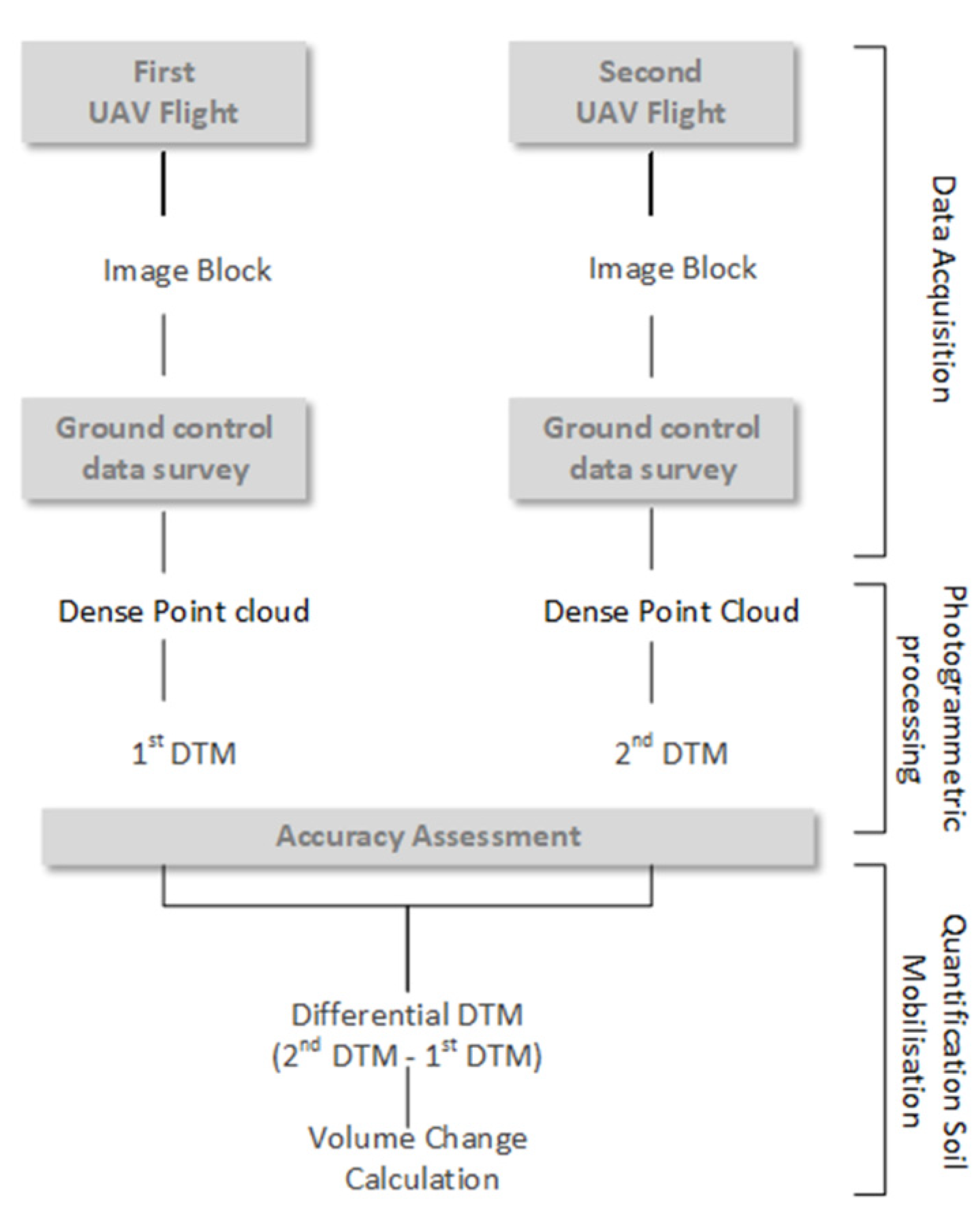
This study proposes a methodology (Figure 1) for the quantification of mobilised soil volume following soil tillage. This methodology is composed of the following three stages: (1) data acquisition, (2) photogrammetry processing, and (3) quantification of soil tillage/mobilisation.

The first stage is related to the acquisition of UAV imagery and ground control survey. The ground control survey is essential to support and improve the positional accuracy of the next stage. The second stage consists of georeferencing each image block based on the photogrammetric SfM workflow, followed by the accuracy assessment. Finally, the last stage has three essential tasks within a volume change workflow: (1) production of a differential DTM grid, containing the elevation difference for every pixel related to the occurred change; (2) correction of differential DTM by unchanged-area-matching method; and (3) calculation of mobilised soil volume from the differential DTM, including the quantification of fill and cut areas (a digital volume model was produced).

The accuracy assessment should be performed at the end of photogrammetric processing and for the 2D/3D products. Both are essential to enable the horizontal and vertical accuracy of results. Positional accuracy should be in the range of one centimetre, taking into account the values that are expected to be estimated for the soil volume mobilisation. Data and process quality control in the whole methodological process are also concerns.

The computing framework was based on the software Agisoft Metashape for SfM processing, and some free and open-source tools from SAGA, GRASS GIS, and QGIS related to raster and statistical analysis were used for co-registration, mapping changed areas, and calculating volume. The use of these GIS tools increases reproducibility and reduces operational costs (available for free use, modification, and distribution) based on the Free and Open Source Software (FOSS) GIS environment.

2.1. Study Area

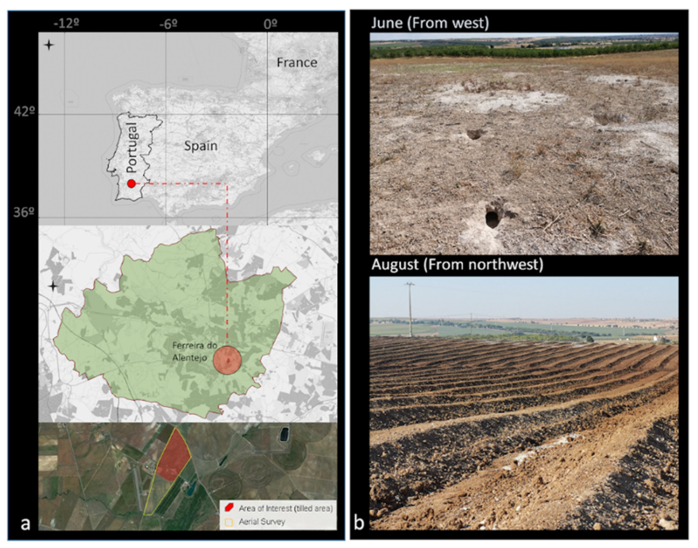
The study area is a rural area located in the small village of Ferreira do Alentejo in the district of Beja, which is approximately 150 km south of Lisbon, Portugal (Figure 2). The total area is approximately 0.55 square kilometres, with an extension of 650 m wide North to South and 400 m long East to West. This rural area can be divided into two areas: the southern area covered by walnut trees and some herbaceous vegetation, and the northern area where a soil tillage operation occurred in August 2019 for olive tree cultivation. The tilled soil area is 187,000 square metres, about 35% of the total area surveyed by UAV.

The collection of UAV data in this area in June and August was easier because it is not a very windy area and the weather in this part of Portugal is temperate with rainy winters and dry, warm summers. Topographically, the terrain has a gentle slope from North to South, with slopes below 10 degrees in 80% of the area of interest.

2.2. UAV Data Acquisition

UAV image acquisition implies completing a series of tasks before flying: (1) choosing sensor or UAV equipment; (2) dealing with administrative procedures, such as flight permissions, pilot licenses, and data collection authorisations; (3) analysing weather conditions (wind and cloudiness); (4) analysing terrain characteristics (vegetation and topography); and (5) mapping flight planning and parameters. In [34], the authors provide a checklist to help users in UAV flight planning and also suggest the metadata for aerial surveys.

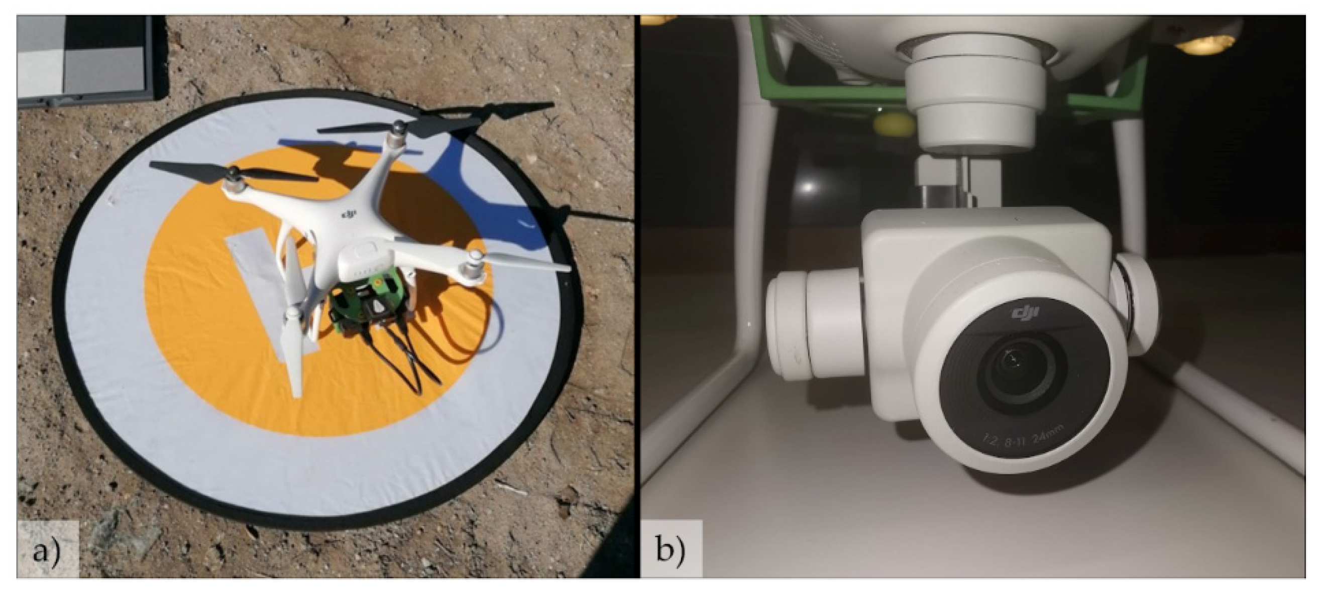
The UAV integrates a direct georeferencing system [35] that includes a GNSS receiver and an inertial navigation system (INS). In practice, this means that the absolute position and orientation parameters of each aerial image are known. The DJI Phantom 4 Pro [36] used in this work is about 1.4 Kg and has a battery autonomy of approximately 20 min (Figure 3) that enabled the coverage of the study area on a single flight. The horizontal and vertical accuracy positioning of onboard GNSS/INS are ±1.5 m and ±0.5 m, respectively [36].

The UAV was equipped with an optical sensor FC6310 (Figure 3b) for RGB data collection, which has a nominal focal length (f) of 8.8 mm and a physical size of 13.2 mm by 8.8 mm. This sensor has a resolution of 20 MPixel (5472 × 3648 pixels) and a pixel size of 2.41 mm. Assuming the characteristics of sensor and flight heights between 100 m and 350 m, the ground sampling distance (GSD) varies from approximately 3 to 10 cm, respectively. The GSD is given by the following equation [37]:

$$\mathrm{GSD}=\frac{\mathrm{H}}{\mathrm{f}}\frac{\mathrm{SS}}{\mathrm{IS}},$$

(1)

where

H: flight height,

f: focal length,

SS: sensor size in pixels,

and IS: image size related to sensor size in pixels.

The amount of UAV flights required to cover a site depends on the size of the area, image overlapping, flight line configuration, GSD, and UAV battery autonomy. For instance, a small GSD leads to longer flight times to cover the entire area of interest.

The study area was covered by two aerial photogrammetric surveys using the same UAV. The first aerial survey was carried out in June 2019, and the second was in August two months later. A very-high spatial resolution (a few centimetres) and higher overlapping imagery were defined for the UAV flight missions, taking into account the objectives of this work.

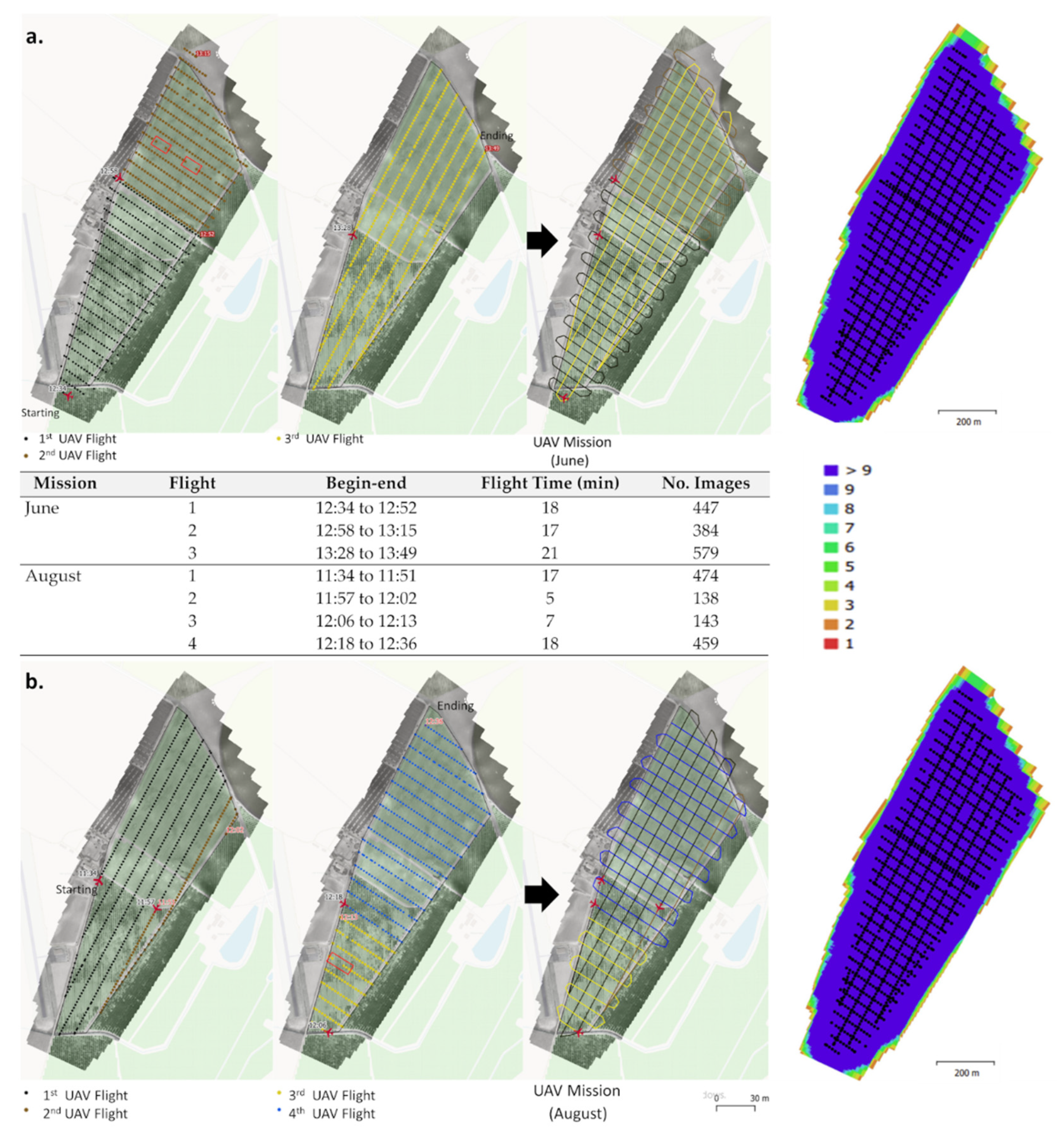
The study area can be covered by one UAV flight in the North–South direction, under suitable conditions of battery life and stable weather conditions with reduced wind. However, the two flight missions made in June and August were planned to enable full coverage of the area, thus reducing the impact of possible camera triggering issues. Therefore, two UAV flights were carried out for each mission (Figure 4): one flight in the North–South direction and the second flight in the opposite direction (West–East). This cross-flight pattern allowed us to increase the point density of the point cloud and provided more details on the topographic surface. Moreover, cross-flight patterns improve camera calibration during image block processing [38] and enhance vertical accuracy in flat and homogeneous terrains [39].

All flights were performed with a forward overlap (between two consecutive images) of about 90%, and the overlap between two consecutive flight lines (side overlap) was about 70% (Figure 4).

The slight variations between exposure cameras that occurred in few areas of image coverage did not contribute to gaps in point cloud (Figure 4) because of the higher overlapping. Usually, these variations result from local disturbances on the UAV system due to wind, radio interference, electro-mechanical failure, etc. [37].

UAV imagery collection with this higher overlapping resulted in at least nine images per object point, without stereoscopic failures, as illustrated in Figure 4. Furthermore, the higher image overlap from multiple point-views and angles contributes to a high level of redundancy and reduces systematic errors [40] in image block photogrammetric processing. In other words, the dense multi-image matching increases the positional quality and point density of the 3D point cloud [41].

It is important to add that the software used to support the flight planning and monitoring of each UAV mission was Map Pilot of DJI. The flight planning was based on the definition of a set of several flight parameters, like some of those mentioned above. The characteristics of UAV flight missions can be seen in

Table 1. Characteristics of the UAV flight missions.

Date	Flying Height (m)	No. of UAV Flights	No. of Flight Lines	GSD (cm/pixel)	No. of Images Taken
27 June 2019	119	3	43	3.1	1410
29 August 2019	117	4	33	3.3	1214

.

Each UAV flight mission (June and August) took one hour approximately with various flights (Figure 4 and Table 1).

For aerial flights, solar altitude is also a relevant factor for the radiometric quality of the imagery. Therefore, low sun angles (<30°) must be avoided to reduce the presence of long shadows and details obscured on images [42]. In this work, the flights were made with a sun angle above 55 degrees of the horizon.

2.3. Ground Control Data Survey

Typically, the direct georeferencing technique (onboard GNSS/IMU) is limited and does not ensure the highest required positional quality [35]. Therefore, the measurement of well-defined points on images—Ground Control Points (GCPs)—for the photogrammetric processing is required to increase the positional accuracy of the image block at the centimetre level [43,44]. Despite some advances in direct georeferencing with the onboard RTK (real-time kinematic) or PPK (post-processed kinematic) positioning technologies, the use of some GCPs is still recommended [42,45].

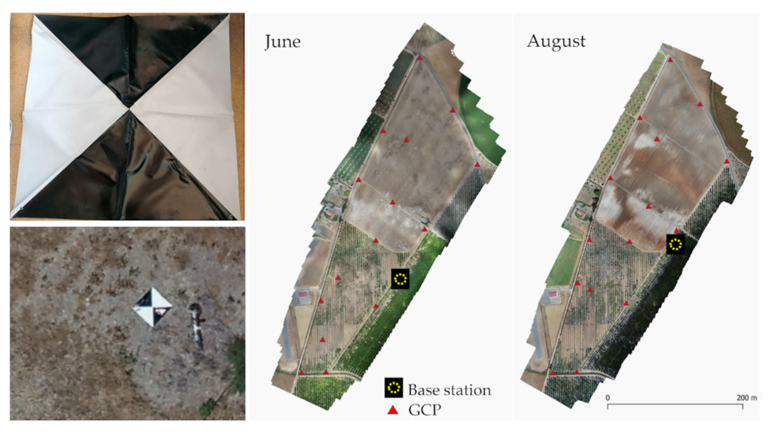
Usually, man-made or natural features can be used as GCP in the area covered by aerial image pairs. However, in this study area, well-defined points were difficult to find as it is a rural area. Therefore, artificial targets of 1 by 1 metre were placed in the area (Figure 5) in June and August. The targets designed were plastic bands with a black and white triangular pattern, with contrasting colours in the centre. Additionally, they were stuck with hooks on the ground to avoid any shift of these plastic bands during the operational flight.

We should highlight that the GCP network established and measured was not the same for the two time periods, including the base station.

It is essential to ensure a good definition of these points in the images for accurate measurements of their image coordinates in the photogrammetric processing as otherwise the positional accuracy of the DSM/DTM would be affected. Although the smallest identifiable object in the image is related to the GSD, the dimension of these points should be slightly higher than the GSD to ensure their clear identification and measuring on images. Assmann et al. [46] recommended an overall side length 7–10 times the GSD for the dimension of these types of square targets. Therefore, the size of artificial targets should not be smaller than 21 cm, considering the GSD imagery. Additionally, these square targets (1 by 1 m) can enable accurate measurements of image coordinates at their mark centre for a GSD of up to 10 cm or a maximum flight height of about 360 m (Equation (1)).

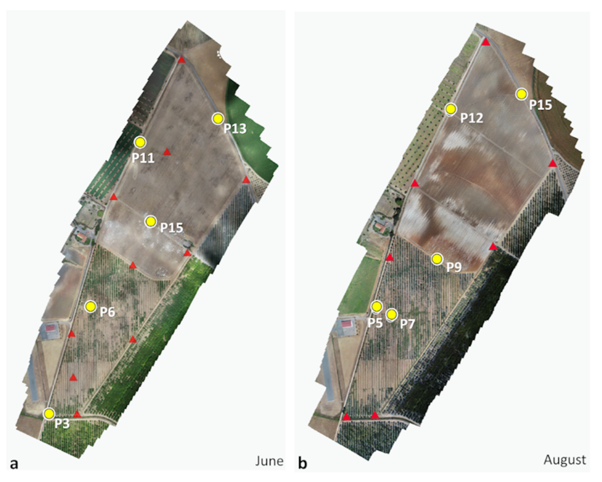
In addition, the accuracy of the field measurements of these targets is also critical for the positional quality of DTM. The position of these 15 target centre points evenly distributed along the area of interest (Figure 5) was accurately measured with a low-cost GNSS system, Emlid Reach RS+ GNSS receiver. According to the manufacturer’s specifications, Emlid’s accuracy is ±0.007 m + 1 ppm horizontal and ±0.014 m + 2 ppm vertical for a single baseline of up to 10 km.

The RTK performance of Emlid is adequate for this work, following the requirements to achieve centimetre-level accurate measurements, viz. (1) the baseline length (distance between the rover and the base station) should be up to 10 km—this is essential because the Emlid system only receives satellite signals on one frequency (L1), which means that positional accuracy decreases at the rate of 1 mm/km [47]; (2) fixing the position derived from measuring, which needed more time for a single-frequency receiver as Emlid. More details about this low-cost device’s usage, accuracy, and limitations can be found in [48].

The coordinate measurements were performed in RTK mode for both surveys, whose distance from the base station to the rover was not more than 1 km. Some of these artificial target points were used as independent check points (ICP) for the accuracy assessment of photogrammetric end-products, which means that they were not included in the processing of UAV data.

It is important to highlight that the assessment of the need for artificial points on the ground should take place before the UAV flight. Another solution is to place some GCPs materialised outside the tilled area, which means that the area can be more easily monitored in the future using the same GCPs.

2.4. Photogrammetric Processing

Photogrammetric processing is an automated image-based reconstruction that combines computer vision and photogrammetric techniques. The photogrammetric mapping includes a range of 2D/3D products, such as dense point clouds, 3D surface models (DSM, DTM), and orthoimages.

Several commercial software products and FOSS photogrammetric solutions have been developed for the automatic processing of UAV imagery. In this study, 3D data were acquired from Agisoft Metashape, commercial software that provides a photogrammetric workflow based on Structure from Motion–Multi-View Stereo (SfM–MVS) for image-block processing.

SfM is a photogrammetric technique that generates a dense point cloud from overlapping images. SfM has revolutionised traditional photogrammetry [40] because it enables the identification and matching of pixels in images at different scales and orientations, including self-camera calibration, and it can produce a georeferenced 3D point cloud without GCPs (using the information of direct georeferencing in the mathematical model).

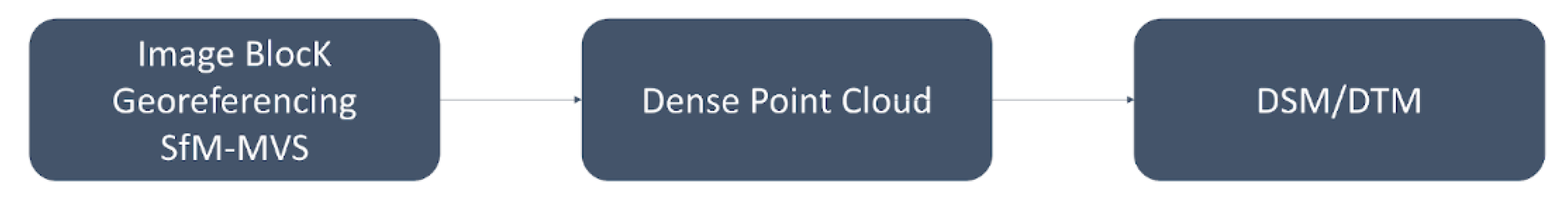
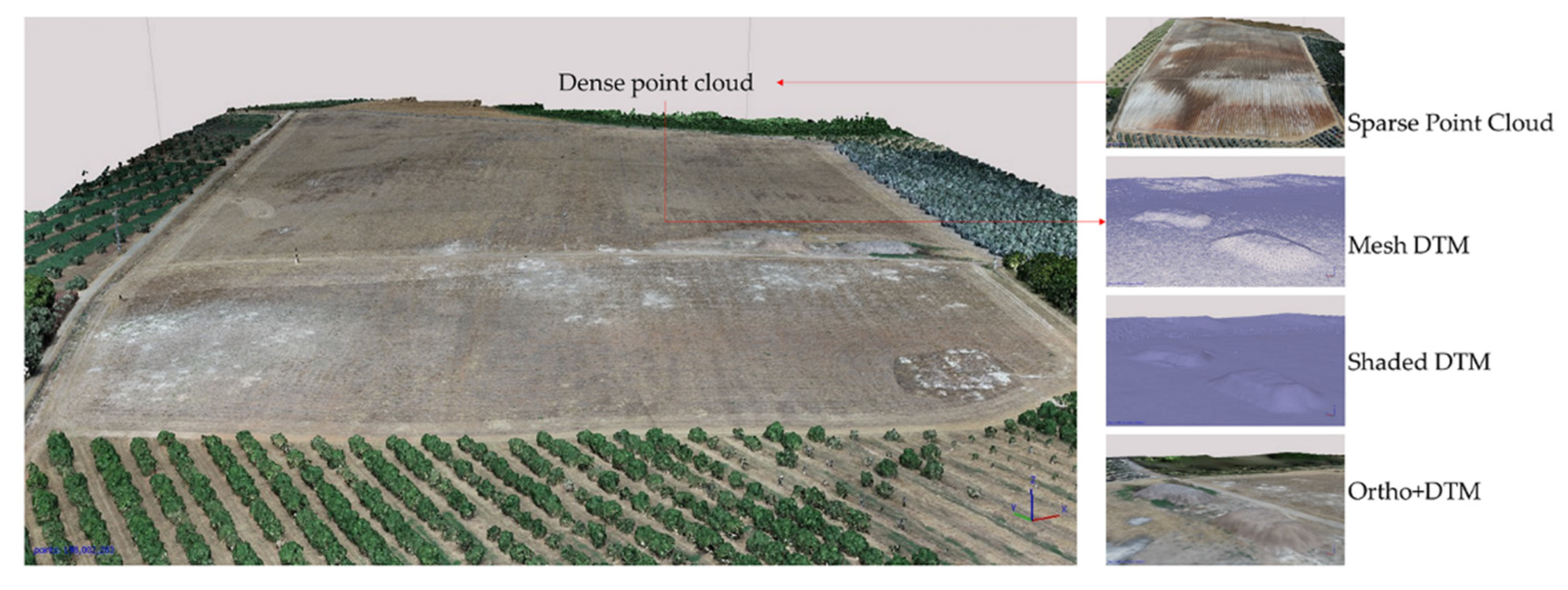
The three main steps of photogrammetric processing used for the production of DSM/DTM are (1) image block georeferencing, (2) dense point cloud generation, and (3) derived DTM from filtering DSM (Figure 6).

Georeferencing is the reconstruction of image block geometry at the exposure time, following the basic principles of aerial triangulation, where camera self-calibration and bundle block adjustment (BBA) were performed within a SfM photogrammetric workflow [40,49].

At the beginning of processing, an initial “alignment” of image pairs is performed using a scale-invariant feature transform (SIFT) approach [50], in which a set of key points identified and matched (tie points) are automatically extracted from the image pairs that overlap. Then, the SfM performs bundle adjustments to compute the camera interior orientation (IO) parameters (including lens distortion), the six exterior orientation parameters (related to the position and orientation of each image captured), and a sparse 3D point cloud (set of tie points). During the BBA step, the image coordinates of a set of GCPs (evenly distributed along the study area) are measured in all image pairs where they appear. In practice, this task is performed simply to correct the position of these points in the images because the block has already undergone an initial alignment from the onboard navigation system. We should also stress that to enable the positional accuracy of block georeferenced and derived products, the usage of a reasonable number of well-defined GCPs with an optimal spatial distribution near image block borders is crucial, as well as some additional GCPs in the middle [42,44,51,52].

Self-camera calibration is also performed in this processing with the initial correction of IO parameters and addition of parameters; in the case of Agisoft Metashape, Brown’s distortion model is used [53].

In sequence, every task involved in the imagery processing contributes to the level of accuracy of an end-product. For instance, sub-pixel accuracy in image-matching, accurate set of GCPs (centimetre-level accuracy) measured in image pairs, and exact camera calibration contribute to a positional accuracy of a few centimetres.

The georeferenced sparse point cloud is densified using an MVS dense matching algorithm. The result is a dense point cloud with RGB information derived from the input images. Finally, the dense point cloud classified as non-ground and ground points was interpolated into a DTM. The grid resolution of the DTM should not be smaller than the point spacing, which is given by the square root of the inverse point density (pts/m2).

The DTM represents the elevation of the bare earth; both artificial and natural objects are excluded. The filtering technique applied for point cloud classification is essential to obtain accurate terrain modelling without errors, and without information that does not belong to the terrain [54], since they influence the estimation of volume changes [55]. Agisoft [53] implemented a ground point filtering, which included a threshold parameter related to the maximum angle between the terrain model and the line to connect the point (15 degrees by default) and the maximum distance parameters for a set of surrounding points. Higher values of the angle parameter may improve results in steeper areas. The accuracy of DSM/DTMs produced from this software is detailed in [43].

In this work, an orthoimage mosaic was also produced using a high-resolution DTM and georeferenced image block. This product was obtained to support the visual inspection of the study area.

2.5. Positional Accuracy

Positional accuracy is a mandatory issue in the UAV mapping of any geospatial product [51]. As one of the measures to assess spatial data quality [56], it reflects the spatial proximity of an element represented in a system from the “true position” or more accurate position. This discrepancy represents a positional error (e_i). Therefore, the positional accuracy of spatial data can be evaluated by the root mean square error (RMSE) statistic [51]. Thus, the horizontal accuracy is assessed by planar RMSE_XY for both directions x and y in Equation (2), and vertical accuracy of 3D data by RMSEz in the z-direction given by Equation (3).

$${\mathrm{RMSE}}_{\mathrm{XY}}=\sqrt{\frac{{\sum }_{\mathrm{i}=1}^{\mathrm{n}}\left(e_x^2{}_i+e_y^2{}_i\right)}{\mathrm{n}}}$$

(2)

$${\mathrm{RMSE}}_{\mathrm{Z}}=\sqrt{\frac{{\sum }_{i=1}^n{e}_z^2{}_i}{n}}$$

(3)

where

n: number of independent checkpoints used;

and $e_x, e_y, e_z$ are positional errors in x, y, and z directions, respectively.

It represents the difference between the estimated coordinate from SfM and the coordinate value obtained from an independent source of higher accuracy (GNSS) for identical ground points; n is the total number of observations.

In practice, the assessment follows the traditional method of comparing estimated and measured ground coordinates for GCPs or ICPs. The ICPs were used to assess the quality of the georeferenced dense point cloud and the DTM at the end of UAV imagery processing. The accuracy assessment of georeferenced image blocks and the DTMs will be discussed in Section 3.2.

2.6. Quantification of Mobilised Soil Volume

Measuring the amount of mobilised soil after tillage implies calculating volume changes for the time frame studied (before and after soil tillage). Among the various methods available for mapping volume changes, the differential DTM was the solution chosen, taking into account UAV-based RGB imagery.

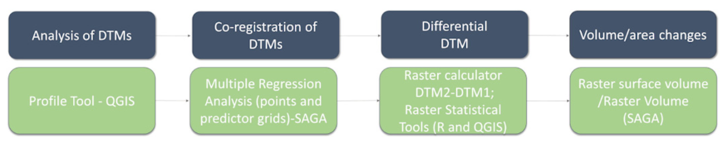
The quantification of mobilised soil volume from the two previously obtained DTMs involves the following steps: (1) analysis of DTMs; (2) co-registration of DTMs, where the deviation between the two DTMs should be reduced; (3) generation of differential DTM; and (4) estimation of volume/area changes occurred after the soil tillage (Figure 7).

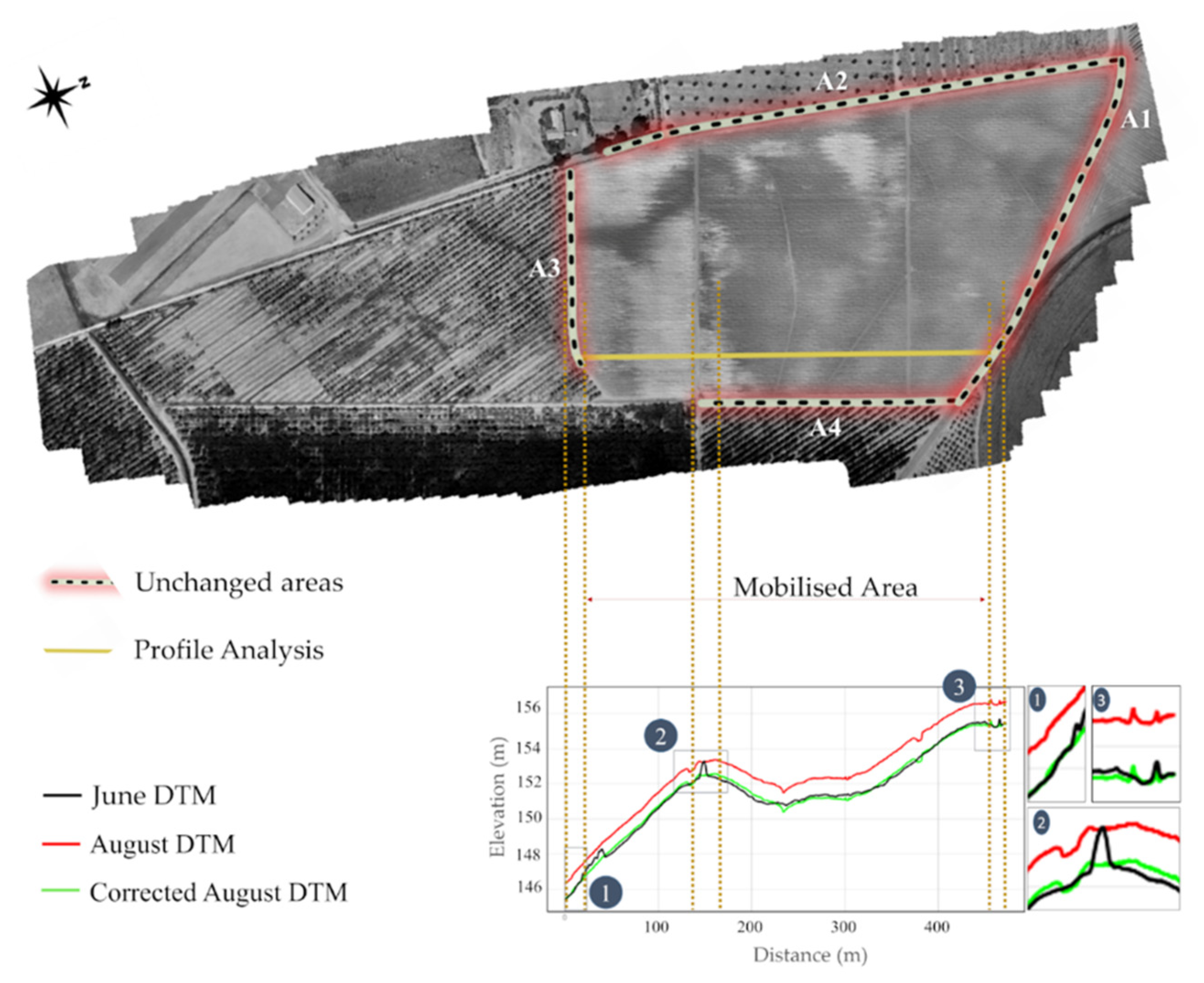
Analytical methods to support the analysis of various DTMs are essential, such as the traditional terrain profiles and the swath profile method [57,58]. In this study, the visual checking of DTM errors and analysis of deviations between the two DTMs were performed with terrain profiles using the QGIS plugin profile tool. Additionally, raster statistical tools from GRASS GIS (r. stats) and QGIS (raster layer statistics) were used to compare the range of elevation values in the two DTMs.

The differential DTM should be derived from the difference between two DTMs with the same resolution, position, and size. This 3D model contains information about the elevation difference for each grid cell data.

The differential DTM provides reliable results if the two following conditions for the input DTMs are met [55]: (1) pixel size, height ranges, and corner coordinates are the same; and (2) the number of free-cut areas and their location match.

Usually, the difficulties in the estimation of accurate volume changes are (1) the uncertainties of input DTMs, related to the quality of point cloud georeferencing and point cloud classification; and (2) the relative co-registration quality of different DTMs (ensuring that in unchanged areas the terrain profiles are almost coincident). The result of differential DTMs never reflects the actual scenario of changes if the issues mentioned above have not been controlled. Several methods have been used to ensure (or improve) the quality of mapping relative changes or volume changes based on correction of relative position between multi-temporal 3D data at the point cloud or DTM levels, such as (1) co-registering point clouds using stable areas, such as roads (using the CloudCompare software) before the generation of the two DSMs [22]; (2) using SIFT key points to detect and match functions (in OpenCV) for the co-registration of raster DSMs [59]; (3) aligning dense point clouds by fitting a reference plane using CloudCompare software [31]; and (4) estimating a mean depth value for differential DTMs, applied for the estimation of a landslide volume [60] in areas of difficult and restricted access.

It is important to highlight that most studies related to the measurement of erosion and landslides consider the same ground control network for the imagery processing and accuracy assessment of DTMs [19,23,24], which allows one to reduce the uncertainties and avoid the alignment of DTMs. However, in our study, the two DTMs were not produced with the same GCPs, because it was not possible to materialise these points due to soil mobilisation. This limitation contributes to a misalignment error between the DTMs.

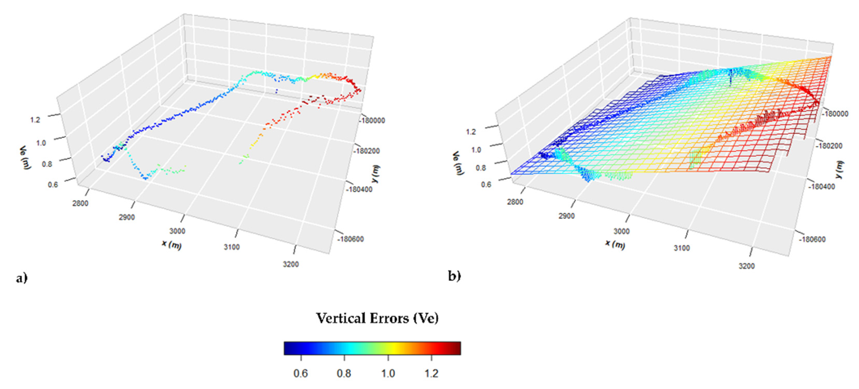
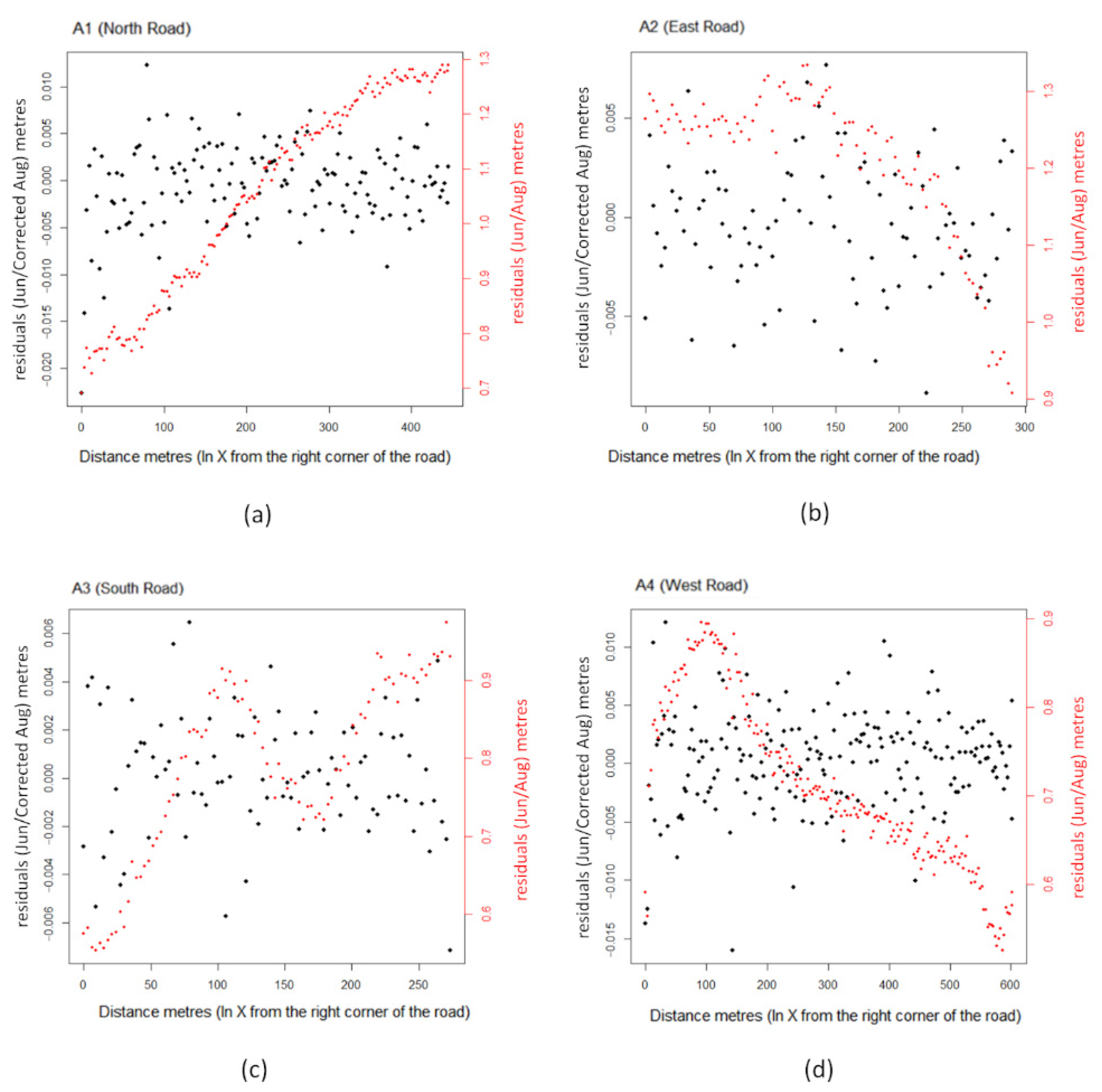
In this work, before the generation of the differential DTM, the relative position between the two DTMs was improved using the unchanged-area-matching method. This method is similar to the co-registration techniques described in previous studies [28,29,61]. Ideally, the DTMs should be coincident in areas where no changes have occurred between the time frames studied. Therefore, the proposed method uses a multiple regression analysis model to reduce the elevation differences in corresponding points of the two DTMs in unchanged areas. The modelling is based on a set of June elevation values related to unchanged areas, where the August DTM (grid) is the dependent variable. The multiple regression model with three independent variables is given by the following equation:

$$Z_{Aug}=\alpha +{\beta }_1{Z}_{Jun}+{\beta }_{2}X+{\beta }_{3}Y\mp \epsilon$$

(4)

where

Z_Jun,: predictor variable related to the elevation data of June profiles,

X$, Y$: predictor variables related to the horizontal coordinates,

$\alpha$: value of Z_Aug when all the other parameters are set to zero (the intercept),

${\beta }_i$: regression coefficients of the corresponding independent variables,

and $\epsilon$: model error (residuals).

The residuals represented in the regression equation by the model error is the difference between the observed and the estimated elevation values of August.

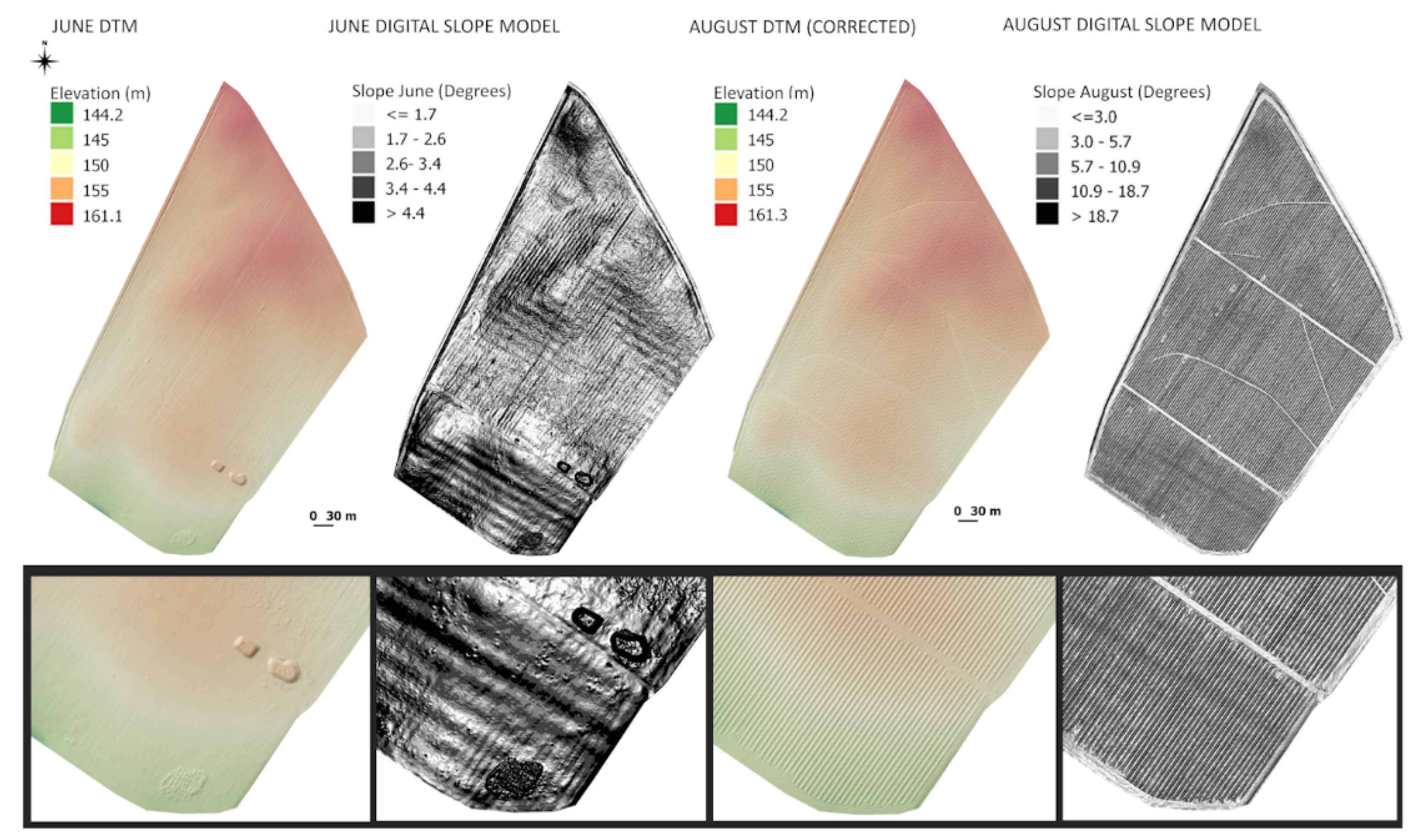
This regression analysis was performed by the multiple regression analysis (points and predictor grids) module implemented in SAGA [62]. First, the regression coefficients were estimated from June elevation profiles of unchanged areas and the August DTM, where the horizontal coordinates were included; second, a new August DTM was produced using the estimated regression model, where the residuals were interpolated onto a regular grid using the bicubic spline interpolation method. The DTM resampled with regression-based values will be called corrected August DTM. The elevation values of corrected August DTM should be closer to the elevation values of June for unchanged areas, as expected (or residuals closer to zero).

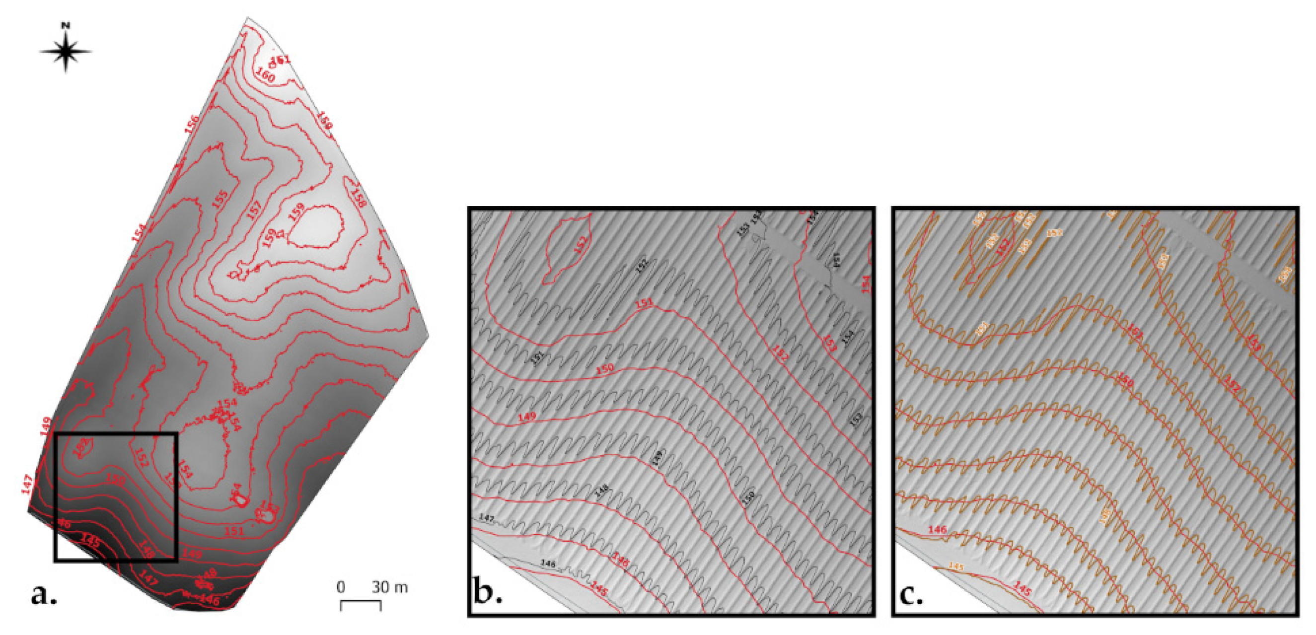
The unchanged areas chosen in the DTMs should be roads or areas with objects above the surface accurately removed by point cloud filtering. It is recommended not to select crop areas or dense vegetation areas when the time frame between the two DTMs is too long to reduce the contribution of inaccurate filtering.

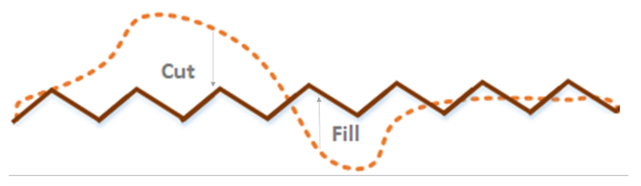
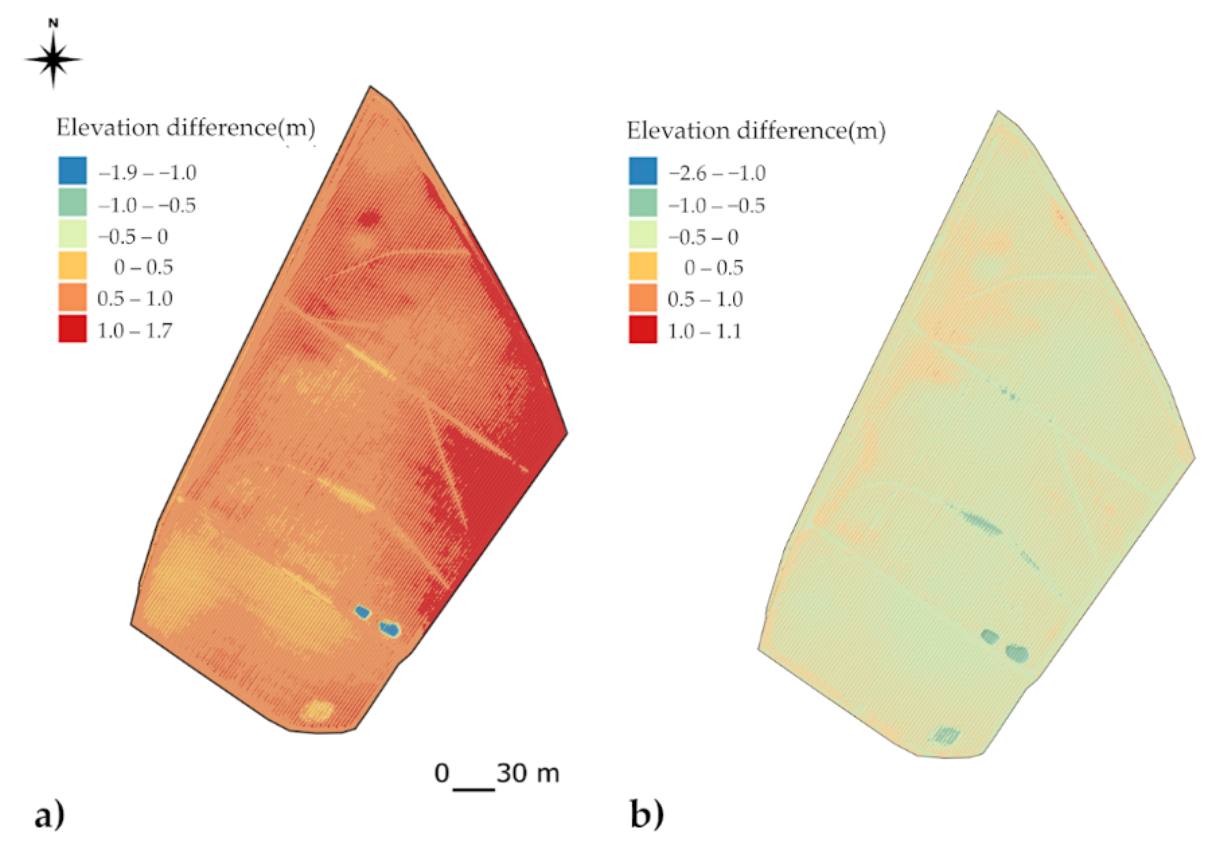
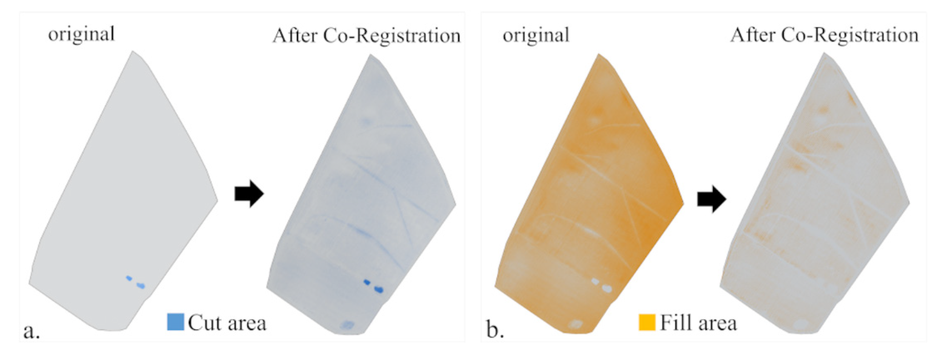
The differential DTM was obtained by subtracting the June DTM from the corrected August DTM using the raster calculator tool in QGIS. This 3D model enabled the identification of the areas where the soil was extracted (cut) or accumulated (fill) in a soil tillage operation (Figure 8). Then, the positive values of the differential DTM grid mean that the terrain elevation has increased or has been filled in August, and negative values indicate that the terrain elevation has decreased or has been cut in August.

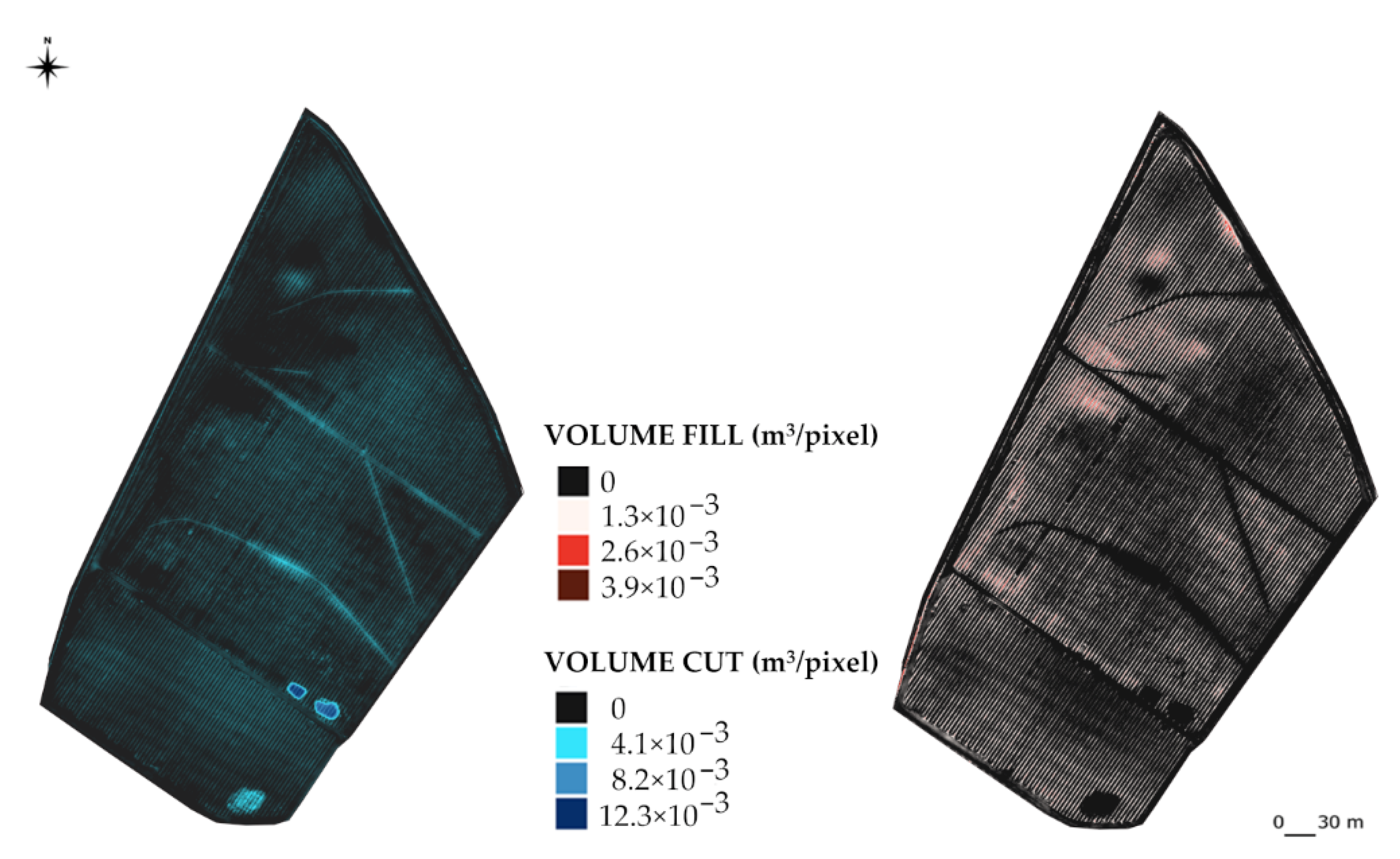
The total mobilised soil volume [V_T] was calculated separately for every pixel that represents fill or cut areas. In practice, it corresponds to the difference between fill and cut volumes. The volume change formula calculated for every differential DTM pixel is given by the following equation:

$$V_T={\displaystyle \sum }_{\mathrm{i}=1}^{\mathrm{n}}{GR}^2{\times h}_i-\left|{\displaystyle \sum }_{j=1}^{m}G{R}^2\times h_j\right|$$

(5)

where

n, m: number of cells for the fill and cut areas, respectively,

GR²: area of each cell, which is given by the grid resolution of Differential DTM,

and h: elevation difference.

The total volume of transferred soil during the soil tillage operation is given by the sum of fill and cut volumes. The digital volume change model was also generated in this work, where each cell grid represents the volume change value. It implies multiplying the differential DTM cells by each cell area on the ground.

The differential DTM, digital volume change model, and the extraction of statistical values were carried out by a set of algorithms dedicated to the analysis and statistical raster grid surface within an environmental QGIS, such as raster volume and raster surface volume.

3. Results and Discussion

The results obtained from the methodology proposed will be presented and discussed in the following sections. Georeferenced image block and DTM accuracy assessment will be discussed in detail. Following the accuracy assessment, the results for the estimation of volume changes will be presented to answer the question: “What is the impact of the co-registration method in Differential DTM quality for the calculation of mobilised soil volume?”

3.1. Imagery Processing and 3D Models

The photogrammetric processing of each UAV image block was made for higher full automation, which required longer processing (about one day and a half of processing for this case study) but enabled a more detailed and accurate dense point cloud for the generation of a high-resolution DTMs. Moreover, in the dense point cloud reconstruction step, a noise filter or “depth filtering“, included in Agisoft [53], was selected for both processing operations. A “mild-depth filtering” [53] was selected for the June image block because there were small mounds or clumps of granular soil that should not have been sorted out as outliers and spatially distinguished in the scene to be reconstructed. For the August image block, a “moderate depth filtering” [53] was applied to the tilled soil (more spatially homogeneous). The main results of the UAV image blocks processed can be seen in

Table 2. Results of SfM processing for each image block (June and August).

	June 2019	August 2019
No. of Images processed	1412	1214
Tie Points	1,327,544	863,682
Reprojection error (pixels)	0.6	0.5
No. of points in the dense point cloud	198,002,283	134,610,431
Point Density (pts/m2)	261	204
Point Spacing (cm/pixel)	6.2	7.0

.

An automatic inspection of aerial image quality was made before the beginning of SfM processing; for both checks, no images were removed (Table 2) from the UAV image block (the quality ranged from 0.8 to 1).

In the re-alignment stage, 15 markers were identified for the June image block (10 GCPs and 5 ICPs) and 12 markers (7 GCPs and 5 ICPs) for the August image block (Figure 9). The GCPs must be used to improve the positional accuracy of georeferencing point clouds from metres to centimetres [43], and consequently, the DTM accuracy. The GCPs used were well-distributed throughout the study area along the block on the margins and in the corners of the area surveyed.

For both processing operations, the sparse point clouds (Figure 10) obtained at the end of georeferencing had no gaps and ranged between several hundred thousand and one million three hundred tie points (Table 2). Finally, the high-density point cloud allowed us to produce a high-resolution DTM with a cell size of 0.07 m using a resampling algorithm included in Agisoft. The results of UAV processing can be seen below (Figure 10).

3.2. Accuracy Assessment

The positional accuracy assessment, horizontal and vertical, is a mandatory procedure. It should be evaluated at the end of the SfM processing for (1) georeferencing; and (2) DTM, or DSM obtained from the georeferenced block.

3.2.1. Georeferencing UAV Image Blocks

The quality of the georeferenced image blocks depends on various factors such as image radiometric quality, flight line configuration, overlapping quality, camera calibration, number of GCPs and their distribution in the image block, GCP positional accuracy, accurately measured GCPs in all image pairs where they appear, processing parameters, and point cloud filtering. For instance, inaccurate GCP measurements in image pairs and inaccurate ground coordinates will affect georeferencing quality significantly.

This study measured the GCPs in mode RTK following the required technical conditions to achieve centimetre-level accuracy. Therefore, two receivers (base station and rover) were included with a base station connected to a National Continuously Operating References Station (CORS) called RENEP, allowing an accuracy better than 10 cm for each GCP measured.

For each image block georeferencing process (June and August): (a) the overlapping for the area of interest was higher than nine images, and no gaps were identified; (b) self-camera calibration parameters and errors were of a few microns; and (c) the tie points were captured with a mean reprojection error less than one pixel (Table 2), which means that the sparse point cloud met the positional accuracy required by standards or the IO and EO parameters were estimated with higher quality.

Both georeferenced dense point clouds achieve a positional accuracy very close to a few centimetres (

Table 3. RMSE values (in cm) computed from the positional errors between estimated GCP (obtained from SfM processing) and field-measured GCP.

RMSE	June 2019	August 2019
XY	5.9	3.1
Z	6.9	8.3
Total	9.2	8.8

). For the June block, the horizontal accuracy is twice less accurate than for the August block, with an RMSE_XY value of about 6 cm (Table 3). On the other hand, the vertical accuracy was slightly better than for the August block, with an RMSEz value of about 7 cm, minus 1.4 cm than the August RMSEz value.

The level of accuracy achieved means that (1) the geometry of image blocks was successfully reconstructed and (2) the georeferenced point cloud obtained will allow the production of a DTM/DSM with a few centimetre-accuracy required for the estimation of mobilised soil volume.

3.2.2. Positional Quality: DTM

DTM accuracy was evaluated using the RMSE calculation based on ICP errors. Then, the horizontal and vertical errors obtained for the five ICPs identified were calculated by ICP-to-raster comparison. For the vertical error, ICP elevation on the DTM produced was compared with ICP elevation measured by GNSS. This task was implemented on an automatic geoprocessing model using a set of QGIS algorithms, included in the GRASS GIS v.what.rast algorithm.

The positional errors obtained were used to calculate the mean absolute error (

Table 4. Positional errors between ICP coordinates estimated from SfM processing and ICP observed (values in centimetres), and mean absolute error (MAE).

ICP	June 2019			ICP	August 2019
	X	Y	Z		X	Y	Z
P3	−2.9	−3.0	−4.1	P5	1.5	1.7	9.9
P6	12.6	2.7	10.9	P7	−0.1	−1.2	−5.4
P11	1.0	7.8	15.9	P9	−1.7	−0.7	13.2
P13	−3.0	−2.5	10.6	P12	−2.6	5.8	3.5
P15	−4.0	2.8	−12.7	P15	−0.4	−2.0	10.1
MAE	3.8	3.2	10.8	MAE	1.3	2.3	8.4

) and RMSE values (

Table 5. RMSE values (in cm) computed from the positional errors obtained for ICPs.

RMSE	June 2019	August 2019
XY	7.2	3.3
Z	11.5	9.1
Total	13.5	9.7

). For the August DTM, the magnitude of positional errors given by mean absolute error (MAE) was slightly lower than for the June DTM (Table 4), with 1.3, 2.3, and 8.4 centimetres for easting(X), northing (Y), and elevation (Z), respectively.

Prior usage of GCPs in the UAV image processing was fundamental to obtain this accuracy of centimetres for the DTM, which without GCPs would be of some metres. Several SfM processing operations were performed for each block based on different scenarios—changing the number of GCPs and their disposition—to get the higher vertical accuracy possible. During this task, four less reliable GCPs were removed from the SfM processing of the August block as the RMSEz values would range between 50 cm and 1 m. In addition, measuring the GCPs on every image where they appear was also relevant to achieve the required accuracy level.

Table 5 shows that the horizontal and vertical accuracy were of centimetres for both DTMs. The RMSExy values were about 7 cm for the June DTM and 3 cm for the August DTM, and RMSEz values for June and August DTMs were 13.5 cm and 10 cm, respectively (Table 5).

Vertical accuracy for both DTMs was similar. This proximity was essential to reduce the effects of a less accurate DTM in estimating changes in elevation after soil preparation.

Compared with other similar studies that aim to quantify soil movement (erosion or accumulation) related to landslides or erosion studies, the vertical accuracy of the DTMs was slightly higher. Gillan et al. [24], Sestras et al. [23], and Gong et al. [19] had RMSEz values for DTMs that ranged from approximately 2 to 3 cm. Gillan et al. had produced a DTM with an RMSEz value of 2.3 cm using GCPs measured with a total station. Goong and Sestras achieved RMSE_Z values of 1.6 cm and 2.7 cm, respectively. Both used higher spatial resolution imagery (1.8 cm and 1.0 cm, respectively) to generate DTMs. DTMs with RMSEz values ranging from 2.7 to 4.6 cm are obtained in Gonçalves et al. [63]. On the other hand, the GCPs were measured with higher precision equipment using dual-frequency GNSS or total station for all these mentioned studies.

Many factors can contribute to DTM accuracy, which makes it challenging to compare studies. Tmušić et al. [34] illustrate well the complexity and the dependence between a large number of factors that can contribute to DTM quality. For instance, some of these factors are (1) the UAV system (sensor and platform type); (2) processing software (parameters of processing, filtering, distribution, and density of the GCPs); (3) environmental conditions at the moment of flight (wind speed, sun-angle, and cloudiness); (4) flight parameters (GSD, flight height); (5) flight planning (overlap, configuration); and (6) GCP positional quality, and the precision of the GNSS equipment used to measure these points.

In our work, during GCP field measurements (August ground survey), we found some difficulties to fix the GNSS observations of some points (it took longer than expected), and the connection to the CORS network was not stable. The vertical accuracy of some GCPs used in SfM processing may not have contributed to higher vertical accuracy (RMSEz < 5 cm). Unfortunately, the use of unmaterialised artificial targets did not enable the repetition of GNSS measurements for a better understanding of these results. However, considering the nature of the soil changes that we intended to estimate, the RMSE values (Table 5) indicated that the DTMs had the positional quality required for this task.

However, it is recommended for DTM accuracy assessment to increase the number of ground points or to use accurate vector data for better quality control. For these studies related to differential DTM, it is important to place a materialised GCP network on the ground distributed evenly across the entire area but outside the area that will be the target of a tillage operation. On the one hand, this ground control network will allow us to use identical ground points for both surveys to ensure the same ground reference for block georeferencing and thus reduce the positional errors on the differential DTMs. On the other hand, it will allow us to improve the unchanged-area-matching method.

3.3. Quantification of Mobilised Soil Volume

The differential DTM was calculated by subtracting the June DTM from the August DTM only for the area of interest (AOI) where the soil tillage was performed. The first analysis of these two DTMs was based on a set of terrain profiles that intersected the unchanged areas (Figure 11), where significant deviations were not expected. This checking profile allowed us to identify a deviation between the two DTMs of about one metre. This deviation evidenced a systematic error between the two DTMs, which may have been caused by (a) the fact that both image block processing operations were not based on the same ground control network and (2) the base station was not identical for both ground surveys.

The correction of this deviation should be performed using a co-registration method to enable the reliable estimation of mobilised soil volume. To better understand the importance of this study, how the co-registration of DTMs is crucial for the accurate measurement of soil tilled volume will be demonstrated and discussed in this section.

3.3.1. Co-Registration of DTMs

The unchanged-area-matching method allowed us to estimate the vertical error between these two DTMs for each corresponding pixel of the unchanged area selected and correct the August DTM with these errors. Four unchanged areas were selected (Figure 11 and

Table 6. Mean elevation and mean elevation difference for each unchanged area.

Unchanged Areas	No. of DataPoints	Mean Elevation June DTM (m)	Mean Elevation Aug DTM (m)	Mean Elevation Difference (m)
A1	5539	158.03	159.08	1.05
A2	7758	153.74	154.45	0.71
A3	3387	145.76	146.56	0.79
A4	3440	151.01	152.21	1.20
Mean		152.14	153.08	0.94

): a paved road of the north area of interest (A1); and the remaining west, south, and east dirt roads of the area of interest (A2, A3, and A4, respectively). An elevation profile from the June DTM was created for each road, which allowed us to obtain a set of elevation points or one elevation point for each DTM pixel (distance between the consecutive two elevation points was approximately 7 cm).

The mean elevation of profiles (June and August) were obtained for each of these unchanged areas, and then the difference between them was analysed (Table 6). The mean elevation difference between DTMs shows a significant deviation for the A1 and A4 areas (Table 6). The mean elevation difference value obtained for the unchanged areas was 94 cm, showing that the co-registration between the August DTM and the June DTM was needed.

The scatterplot of vertical errors (or elevation difference for each point of the profile) between the August and June profiles can be seen in Figure 12. The higher values were located to the northeast of the A1 and A4 unchanged areas. The simple regression plane also shows approximately the spatial distribution and magnitude of the vertical errors along the tilled area limited by profiles.

The co-registration of the August DTM to the June DTM was performed using a multiple regression analysis of June elevation points (extracted from the unchanged areas) to the August DTM grid. Therefore, the vertical errors for these unchanged areas are expected to be closer to zero.

The horizontal coordinates (X and Y) were also included as independent variables. Since the sample points were taken from the edges of the study area, there was bound to be some degree of directional spatial dependence in the series (W-E or N-S). The non-inclusion of these variables could potentially cause bias in the estimates [64]. Nonetheless, it is worth mentioning that the inclusion of horizontal coordinates as regressors is one of several methods to account for spatial structure in the data [65]. Therefore, the modelling results for the corrected August DTM (${\widehat{Z}}_{Aug})$ were given by the following equation:

$${\widehat{Z}}_{Aug}=-147.10+1.06Z_{Jun}-0.002X-0.001Y\mp \epsilon$$

(6)

The estimated coefficients indicate the magnitude of deviation between the two DTMs obtained from different UAV surveys. As expected, the “June elevation points” variable shows a strong relationship with the estimated August elevation points.

After estimating the regression coefficients, the August DTM was corrected using the regression-based values, where the elevation values on unchanged areas were modelled to the June elevations. Finally, the vertical errors (or residuals) between corrected August and June DTMs were calculated for unchanged areas.

The regression model (Equation (6)) is robust for the co-registration of the August DTM onto the June DTM, based on the analysis of multiple R-Squared, adjusted R-Squared, and residuals (Figure 13). The R-Squared and adjusted R-Squared statistics derived from the regression equation (Equation (6)) were approximately 0.998, which close to 1 indicates good model performance to correct the August DTM. Furthermore, the residuals that represented the vertical errors between the corrected August and June elevations are close to zero (

Table 7. Statistical values for vertical errors (Corrected August DTM–June DTM) of unchanged areas (values in metres).

Vertical Errors	Mean Absolute Error	Min.	Max.	Std. dev.	RMSE
August–June	0.905	0.263	1.786	0.447	0.935
Corrected August–June	0.004	−0.043	0.044	0.005	0.005

and Figure 13), ranging from −0.043 m to 0.044 m.

The August DTM was adjusted to the June DTM (Figure 13) for unchanged areas (Figure 13). This means a good fit of the August DTM in these areas was achieved using the regression model presented in Equation (6).

The MAE of vertical errors was improved from 0.91 m to 0.004 m with the correction of the August DTM. The RMSEz value obtained from this modelling was about 0.005 m (Table 7), indicating the model’s error lower magnitude.

Analysing the area of interest, the difference between the mean elevation of the August DTM and the June DTM decreased from +0.82 m to −0.03 m with this correction (

Table 8. Characterisation of DTMs by elevation values (m) obtained for the area of interest (AOI).

DTM	AOI
	Jun.	Aug.	Corrected Aug.
Mean	153.58	154.40	153.55
Minimum	144.14	145.03	144.17
Maximum	161.19	162.06	161.33

); only in the unchanged areas did it decrease from +0.94 m to 3.74 × 10⁻⁵ m (Table 6). Furthermore, the range of elevation values for the corrected August DTM became closer to the elevation range values of June (Table 8 and Figure 11).

A visual inspection of the relative position of the two DTMs, along x and y, can be made easier using contour lines. This qualitative evaluation allowed us to ascertain that the applied multiple regression model (Equation (6)) is reliable to adjust the DTMs or effective in reducing the presence of horizontal deviation between the DTM dataset (Figure 14).

The above analysis shows that the unchanged-area-matching method effectively aligned multi-temporal DTMs obtained from UAV surveys with the minimisation of uncertainties. However, in previous studies that use the multiple regression model for the co-registration of DEMs obtained from satellite images, the magnitude of errors was higher than the results obtained in this study [28].

The high-resolution of these DTMs produced easily allowed us to identify that conventional soil tillage occurred in August, where a well-defined tilled pattern is shown (Figure 15). In June, 98% of the study area had slope angles of less than 10 degrees, and the mean slope was 3.5 degrees (Figure 15). After the soil tillage operation, the slope angles of less than 10 degrees decreased to 56% of the total area and the mean slope increased to 10.6 degrees. The maximum slopes in June and August were about 63 and 73 degrees, respectively, and occurred along the boundary area of interest.

The analysis of topography and slopes before the soil tillage operation can be useful to quantify the amount of soil that is expected to have been mobilised and simultaneously estimate the costs of the operation. Furthermore, the DTM and the digital slope model can provide a solid basis for management and decision-making, e.g., by answering the question “What tillage method should be applied in an area where the soil is highly erodible, and the slope is very steep?” Additionally, the DTM produced before the soil was tilled allowed us to check the quality of the operation performed, as well as predict erodible areas and flood zones.

In addition, the 3D data obtained before soil tillage can help plan a conventional tillage operation with the optimisation and minimisation of farming machinery traffic, such as reducing the number of trajectories during the soil tillage, taking into account the obstacles and slopes. The development of traffic farming techniques has been addressed by some authors [66,67] to minimise erosion and soil compaction during a conventional tillage operation.

3.3.2. Differential DTM

The comparison between the differential DTM improved by the corrected August DTM and the differential DTM without co-registration is discussed in this subsection, where the impact level of the corrected August DTM in the differential DTM is demonstrated.

The differential DTM results show two very different scenarios regarding the amount of soil that was tilled (Figure 16). The first scenario corresponds to the differential DTM obtained from the two DTMs (without any correction). The second represents the differential DTM corrected by the adjustment of the August DTM to the June DTM using the unchanged-area-matching method. In the corrected differential DTM, the soil tillage is slightly negative (or more area was cut) with a mean elevation difference of about −0.04 m, while the initial differential DTM shows positive soil tillage (or more area was filled) with a mean elevation of +0.82 m (

Table 9. Statistical values for differential DTMs (elevation difference values in metres).

Differential DTM	Mean	Minimum	Maximum
August–June	0.82	−1.90	1.66
Corrected August–June	−0.04	−2.62	1.10

). The elevation difference values for the initial differential DTM varies between −1.90 m (minimum) and +1.66 m (maximum), which after co-registration decreases to −2.62 m and +1.10 m, respectively.

These distinct scenarios estimated show the impact of co-registration made by the unchanged-area-matching method. Access paths created with the soil mobilisation were easily identified on the differential DTM (Figure 16b) with range elevation difference from −0.5 to 0 cm. The northeast part of the differential DTM (Figure 16a) with the highest elevation difference values was corrected for a range between −0.5 and 0.5 cm. The co-registration of the DTMs is fundamental to enable reliable results on the soil tillage operation performed.

3.3.3. Calculation of the Tilled Soil Volume

First, an analysis of the impact of co-registration for the estimation of extracted and accumulated areas resulting from the soil tillage operation was carried out. The cut area change rate increased from 0.3% to 62% with the correction of the August DTM (Figure 17a and

Table 10. Fill and cut volumes and change volume for the different differential DTM scenarios: First scenario—differential DTM without co-registration of input DTMs; second scenario—differential DTM with correction of the August DTM.

Scenarios	Volume	Area (m2)	Change Area (%)	Volume (m3)	Volume Change (m3)
First	Cut	522	0.3%	−517	156,625
	Fill	190,827	99.7%	157,143
Second	Cut	118,756	62.1%	−16,146	−7108
	Fill	72,587	37.9%	9037

). This increase means more than 118,200 m² (more than 61.8% of the total area) of soil was extracted during the tillage operation. The fill area change rate significantly decreased from 99.7% to 37.9% (Figure 17b).

Among the two estimated scenarios for the cut and fill areas, we can also assess the degree of difficulty in carrying out the soil tillage operation. In the first scenario, the difficulty was lower (underestimated) than in the second. For instance, the mechanic work performed in the soil, such as digging, moving, and turning, will be more difficult in the second scenario.

Next, the estimated mobilised soil volume is analysed for these two different scenarios (Figure 17 and Table 10). The co-registration of the DTMs increased the cut volume from −517 m³ to −16,146 m³ and decreased the fill volume from 157,143 m³ to 9037 m³ (Table 10). As a result, the volume change resulting from the tillage operation showed a positive value for the first scenario with 156,625 m³, while in the second scenario, it changed significantly with a negative value of 7108 m³. This means that the volume change was corrected considerably between these two scenarios in absolute values corresponding to minus 163,733 m³.

The soil tillage operation performed in August also shows that about 25,183 m³ of the soil transferred was mobilised in about 190,000 m². This value allowed us to estimate the time spent by a company in the execution of this operation and enabled the estimation of operation costs as a function of the volume transferred (cut and fill volume).

The digital volume change models obtained for this soil tillage operation are shown in Figure 18.

The volume change for each pixel of this model is smaller, taking into account the size area of a pixel on the ground (4.9 × 10⁻³ m²/pixel). The cut volume varies between $4\times {10}^{-3}$m³ and $12\times {10}^{-3}$m³/pixel, and the fill volume from $1\times {10}^{-3}$m³/pixel to $4\times {10}^{-3}$m³/pixel (Figure 18).

These results allowed us to identify the areas where the tillage operation was more intensive, based on higher volume changes. The higher volume changes occurred in the areas (1) closer to mounds of land, which means cutting and then filling the surrounding areas; (2) northwest/west of the study area, due to high variability in the slopes before the tillage operation (Figure 15); and (3) including the dirt road access paths. It also means that the volume changes in these areas resulted in a higher intensity of machinery traffic and thus increased the risk of adverse effects, such as soil compaction.

To validate these 3D models, the usage of a set of GNSS field-measured sample objects is recommended before the soil tillage operation, such as mounds of land.

4. Conclusions

This study showed the potential of UAV data in the estimation of soil volume change for a soil tillage operation. Therefore, a methodology was proposed to manage and monitor land preparation with low costs within a short time, which includes estimating fill/cut volumes and change volumes after the soil tillage with an accuracy level of a few centimetres. It also integrates the positional accuracy assessment of georeferenced UAV blocks and DTMs, where the accuracy of a few centimetres was required for this work. Following the importance of data quality assessment to estimate change volume, the impact of differential DTM co-registered with the unchanged-area-matching method was also demonstrated.

Some improvements must be considered for this proposed methodology: (1) usage of a UAV system that integrates GNSS RTK or PPK to reduce the fieldwork when measuring GCPs, and (2) establishing a materialised GCP network outside the tilled area to ensure the monitoring of future tasks in the same area, and also to reduce (or avoid) the vertical error between multi-temporal DTMs/DSMs.

This work contributes to monitoring soil changes with a methodology that allows us to combine multi-temporal DTMs obtained from different UAV surveys. Furthermore, the usage of multi-temporal UAV data will become a more common procedure and a challenge for data users, which will increase the demand for solutions that allow for the comparison of 3D data. From a farmer’s point of view, it is helpful in monitoring runoff conditions. Moreover, it can be used as an economic model, where the costs of soil tillage operations are based on volume (3D data) instead of area size (2D data).

UAV technology and robust methodologies for the acquisition of 3D models that can be easily implemented and used by farmers in land preparation will bring many advantages when managing and monitoring the effects of traditional and conventional tillage systems, such as reducing soil compaction caused by machinery. Furthermore, it will contribute to sustainable precision agriculture with the usage of efficient geospatial tools, ensuring the data quality of a 2D/3D product.

References

1. Khanal, S.; Kc, K.; Fulton, J.; Shearer, S.; Ozkan, E. Remote Sensing in Agriculture—Accomplishments, Limitations, and Opportunities. Remote Sens. 2020, 12, 3783. [Google Scholar] [CrossRef]
2. Sishodia, R.P.; Ray, R.L.; Singh, S.K. Applications of Remote Sensing in Precision Agriculture: A Review. Remote Sens. 2020, 12, 3136. [Google Scholar] [CrossRef]
3. Hristov, G.; Raychev, J.; Kinaneva, D.; Zahariev, P. Emerging Methods for Early Detection of Forest Fires Using Unmanned Aerial Vehicles and Lorawan Sensor Networks. In Proceedings of the 2018 28th EAEEIE Annual Conference (EAEEIE), Reykjavik, Iceland, 26–28 September 2018; pp. 1–9. [Google Scholar]
4. Park, S.; Ryu, D.; Fuentes, S.; Chung, H.; Hernández-Montes, E.; O’Connell, M. Adaptive estimation of crop water stress in nectarine and peach orchards using high-resolution imagery from an unmanned aerial vehicle (UAV). Remote Sens. 2017, 9, 828. [Google Scholar] [CrossRef] [Green Version]
5. Ahmed, O.S.; Shemrock, A.; Chabot, D.; Dillon, C.; Williams, G.; Wasson, R.; Franklin, S.E. Hierarchical land cover and vegetation classification using multispectral data acquired from an unmanned aerial vehicle. Int. J. Remote Sens. 2017, 38, 2037–2052. [Google Scholar] [CrossRef]
6. Orsini, R.; Fiorentini, M.; Zenobi, S. Evaluation of Soil Management Effect on Crop Productivity and Vegetation Indices Accuracy in Mediterranean Cereal-Based Cropping Systems. Sensors 2020, 20, 3383. [Google Scholar] [CrossRef]
7. Adão, T.; Hruška, J.; Pádua, L.; Bessa, J.; Peres, E.; Morais, R.; Sousa, J.J. Hyperspectral imaging: A review on UAV-based sensors, data processing and applications for agriculture and forestry. Remote Sens. 2017, 9, 1110. [Google Scholar] [CrossRef] [Green Version]
8. Michez, A.; Piégay, H.; Lisein, J.; Claessens, H.; Lejeune, P. Classification of riparian forest species and health condition using multi-temporal and hyperspatial imagery from unmanned aerial system. Environ. Monit. Assess. 2016, 188, 1–19. [Google Scholar] [CrossRef] [Green Version]
9. Quan, Y.; Li, M.; Zhen, Z.; Hao, Y.; Wang, B. The Feasibility of Modelling the Crown Profile of Larix olgensis Using Unmanned Aerial Vehicle Laser Scanning Data. Sensors 2020, 20, 5555. [Google Scholar] [CrossRef]
10. Christiansen, M.P.; Laursen, M.S.; Jørgensen, R.N.; Skovsen, S.; Gislum, R. Designing and Testing a UAV Mapping System for Agricultural Field Surveying. Sensors 2017, 17, 2703. [Google Scholar] [CrossRef] [Green Version]
11. Fu, Z.; Jiang, J.; Gao, Y.; Krienke, B.; Wang, M.; Zhong, K.; Cao, Q.; Tian, Y.; Zhu, Y.; Cao, W.; et al. Wheat Growth Monitoring and Yield Estimation based on Multi-Rotor Unmanned Aerial Vehicle. Remote Sens. 2020, 12, 508. [Google Scholar] [CrossRef] [Green Version]
12. Madsen, S.L.; Dyrmann, M.; Laursen, M.S.; Jørgensen, R.N. RoboWeedSupport-Semi-Automated Unmanned Aerial System for Cost Efficient High Resolution in Sub-Millimeter Scale Acquisition of Weed Images. Int. J. Mech. Mechatron. Eng. 2017, 11, 835–839. [Google Scholar]
13. Dash, J.P.; Watt, M.; Pearse, G.D.; Heaphy, M.; Dungey, H. Assessing very high resolution UAV imagery for monitoring forest health during a simulated disease outbreak. ISPRS J. Photogramm. Remote Sens. 2017, 131, 1–14. [Google Scholar] [CrossRef]
14. Bellvert, J.; Zarco-Tejada, P.J.; Girona, J.; Fereres, E. Mapping crop water stress index in a ‘Pinot-noir’ vineyard: Comparing ground measurements with thermal remote sensing imagery from an unmanned aerial vehicle. Precis. Agric. 2014, 15, 361–376. [Google Scholar] [CrossRef]
15. Radoglou-Grammatikis, P.; Sarigiannidis, P.; Lagkas, T.; Moscholios, I. A compilation of UAV applications for precision agriculture. Comput. Netw. 2020, 172, 107148. [Google Scholar] [CrossRef]
16. Tsouros, D.C.; Bibi, S.; Sarigiannidis, P.G. A review on UAV-based applications for precision agriculture. Information 2019, 10, 349. [Google Scholar] [CrossRef] [Green Version]
17. Kaiser, A.; Neugirg, F.; Rock, G.; Müller, C.; Haas, F.; Ries, J.; Schmidt, J. Small-Scale Surface Reconstruction and Volume Calculation of Soil Erosion in Complex Moroccan Gully Morphology Using Structure from Motion. Remote Sens. 2014, 6, 7050–7080. [Google Scholar] [CrossRef] [Green Version]
18. Neugirg, F.; Stark, M.; Kaiser, A.; Vlacilova, M.; Della Seta, M.; Vergari, F.; Schmidt, J.; Becht, M.; Haas, F. Erosion processes in calanchi in the Upper Orcia Valley, Southern Tuscany, Italy based on multitemporal high-resolution terrestrial LiDAR and UAV surveys. Geomorphology 2016, 269, 8–22. [Google Scholar] [CrossRef]
19. Gong, C.; Lei, S.; Bian, Z.; Liu, Y.; Zhang, Z.; Cheng, W. Analysis of the Development of an Erosion Gully in an Open-Pit Coal Mine Dump During a Winter Freeze-Thaw Cycle by Using Low-Cost UAVs. Remote Sens. 2019, 11, 1356. [Google Scholar] [CrossRef] [Green Version]
20. Raeva, P.L.; Filipova, S.L.; Filipov, D.G. Volume computation of a stockpile—A study case comparing GPS and UAV measurements in an open pit quarry. ISPRS Int. Arch. Photogramm. Remote Sens. Spat. Inf. Sci. 2016, 41, 999–1004. [Google Scholar] [CrossRef] [Green Version]
21. Carabassa, V.; Montero, P.; Crespo, M.; Padró, J.-C.; Pons, X.; Balagué, J.; Brotons, L.; Alcañiz, J.M. Unmanned aerial system protocol for quarry restoration and mineral extraction monitoring. J. Environ. Manag. 2020, 270, 110717. [Google Scholar] [CrossRef]
22. Rauhala, A.; Tuomela, A.; Davids, C.; Rossi, P.M. UAV Remote Sensing Surveillance of a Mine Tailings Impoundment in Sub-Arctic Conditions. Remote Sens. 2017, 9, 1318. [Google Scholar] [CrossRef] [Green Version]
23. Sestras, P.; Bilașco, Ș.; Roșca, S.; Dudic, B.; Hysa, A.; Spalević, V. Geodetic and UAV Monitoring in the Sustainable Management of Shallow Landslides and Erosion of a Susceptible Urban Environment. Remote Sens. 2021, 13, 385. [Google Scholar] [CrossRef]
24. Gillan, J.K.; Karl, J.W.; Elaksher, A.; Duniway, M.C. Fine-Resolution Repeat Topographic Surveying of Dryland Landscapes Using UAS-Based Structure-from-Motion Photogrammetry: Assessing Accuracy and Precision against Traditional Ground-Based Erosion Measurements. Remote Sens. 2017, 9, 437. [Google Scholar] [CrossRef] [Green Version]
25. Barbosa, V.F. Planting. In Sugarcane Agricultural Production, Bioenergy and Ethanol, 1st ed.; Santos, F., Borém, A., Caldas, C., Eds.; Academic Press: Cambridge, MA, USA, 2015; p. 492. ISBN 9780128022399. [Google Scholar] [CrossRef]
26. Cucchiaro, S.; Maset, E.; Cavalli, M.; Crema, S.; Marchi, L.; Beinat, A.; Cazorzi, F. How does co-registration affect geomorphic change estimates in multi-temporal surveys? GIScience Remote Sens. 2020, 57, 611–632. [Google Scholar] [CrossRef]
27. Nuth, C.; Kääb, A. Co-registration and bias corrections of satellite elevation data sets for quantifying glacier thickness change. Cryosphere 2011, 5, 271–290. [Google Scholar] [CrossRef] [Green Version]
28. Peduzzi, P.; Herold, C.; Silverio, W. Assessing high altitude glacier thickness, volume and area changes using field, GIS and remote sensing techniques: The case of Nevado Coropuna (Peru). Cryosphere 2010, 4, 313–323. [Google Scholar] [CrossRef] [Green Version]
29. Gorokhovich, Y.; Voustianiouk, A. Accuracy assessment of the processed SRTM-based elevation data by CGIAR using field data from USA and Thailand and its relation to the terrain characteristics. Remote Sens. Environ. 2006, 104, 409–415. [Google Scholar] [CrossRef]
30. Ashapure, A.; Jung, J.; Yeom, J.; Chang, A.; Maeda, M.; Maeda, A.; Landivar, J. A novel framework to detect conventional tillage and no-tillage cropping system effect on cotton growth and development using multi-temporal UAS data. ISPRS J. Photogramm. Remote Sens. 2019, 152, 49–64. [Google Scholar] [CrossRef]
31. Remke, A.; Rodrigo-Comino, J.; Gyasi-Agyei, Y.; Cerdà, A.; Ries, J.B. Combining the Stock Unearthing Method and Structure-from-Motion Photogrammetry for a Gapless Estimation of Soil Mobilisation in Vineyards. ISPRS Int. J. Geo-Inf. 2018, 7, 461. [Google Scholar] [CrossRef] [Green Version]
32. Paroissien, J.-B.; Lagacherie, P.; le Bissonnais, Y. A regional-scale study of multi-decennial erosion of vineyard fields using vine-stock unearthing–burying measurements. Catena 2010, 82, 159–168. [Google Scholar] [CrossRef]
33. Delgado, J.A.; Short, N.M.J.; Roberts, D.P.; Vandenberg, B. Big Data Analysis for Sustainable Agriculture on a Geospatial Cloud Framework. Front. Sustain. Food Syst. 2019, 3, 54. [Google Scholar] [CrossRef] [Green Version]
34. Tmušić, G.; Manfreda, S.; Aasen, H.; James, M.R.; Gonçalves, G.; Ben-Dor, E.; Brook, A.; Polinova, M.; Arranz, J.J.; Mészáros, J.; et al. Current Practices in UAS-based Environmental Monitoring. Remote Sens. 2020, 12, 1001. [Google Scholar] [CrossRef] [Green Version]
35. Turner, D.; Lucieer, A.; Wallace, L. Direct Georeferencing of Ultrahigh-Resolution UAV Imagery. IEEE Trans. Geosci. Remote Sens. 2014, 52, 2738–2745. [Google Scholar] [CrossRef]
36. DJI. Phantom 4 Pro-User Manual V1.8. DJI. Available online: https://dl.djicdn.com/downloads/phantom_4_pro/20200108/Phantom_4_Pro_Pro_Plus_Series_User_Manual_EN.pdf (accessed on 20 July 2021).
37. Grubesic, T.H.; Nelson, J.R. Legal, Environmental, Operational, and Safety Challenges in Urban Areas. In UAVs Urban Spatial Analysis: An Introduction; Grubesic, T.H., Nelson, J.R., Eds.; Springer International Publishing: Berlin/Heidelberg, Germany, 2020; pp. 51–69. [Google Scholar] [CrossRef]
38. Przybilla, H.-J.; Bäumker, M.; Luhmann, T.; Hastedt, H.; Eilers, M. Interaction between direct georeferencing, control point configuration and camera self-calibration for RTK-based UAV photogrammetry. ISPRS-Int. Arch. Photogramm. Remote Sens. Spat. Inf. Sci. 2020, 43, 485–492. [Google Scholar] [CrossRef]
39. Gerke, M.; Przybilla, H.-J. Accuracy Analysis of Photogrammetric UAV Image Blocks: Influence of Onboard RTK-GNSS and Cross Flight Patterns. Photogramm. Fernerkund. Geoinf. 2016, 2016, 17–30. [Google Scholar] [CrossRef] [Green Version]
40. Iglhaut, J.; Cabo, C.; Puliti, S.; Piermattei, L.; O’Connor, J.; Rosette, J. Structure from Motion Photogrammetry in Forestry: A Review. Curr. For. Rep. 2019, 5, 155–168. [Google Scholar] [CrossRef] [Green Version]
41. Haala, N.; Cramer, M.; Rothermel, M. Quality of 3D point clouds from highly overlapping UAV imagery. ISPRS Int. Arch. Photogramm. Remote Sens. Spat. Inf. Sci. 2013, 183–188. [Google Scholar] [CrossRef] [Green Version]
42. Wolf, P.R.; Dewitt, B.A.; Wilkinson, B. Elements of Photogrammetry with Applications in GIS, 4th ed.; McGraw-Hill: New York, NY, USA, 2014; p. 696. ISBN 9780071761123. [Google Scholar]
43. Muji, A.L.; Tahar, K.N. Assessment of Digital Elevation Model (DEM) using onboard GPS and ground control points in UAV image processing. In Proceedings of the Intelligent Systems Conference (IntelliSys), London, UK, 7 September 2017; IEEE: New York, NY, USA, 2017; pp. 835–842. [Google Scholar]
44. Sanz-Ablanedo, E.; Chandler, J.H.; Rodríguez-Pérez, J.R.; Ordóñez, C. Accuracy of Unmanned Aerial Vehicle (UAV) and SfM Photogrammetry Survey as a Function of the Number and Location of Ground Control Points Used. Remote Sens. 2018, 10, 1606. [Google Scholar] [CrossRef] [Green Version]
45. Forlani, G.; Diotri, F.; di Cella, U.M.; Roncella, R. UAV Block Georeferencing and Control By On-Board GNSS Data. ISPRS-Int. Arch. Photogramm. Remote Sens. Spat. Inf. Sci. 2020, 43, 9–16. [Google Scholar] [CrossRef]
46. Assmann, J.J.; Kerby, J.T.; Cunliffe, A.M.; Myers-Smith, I.H. Vegetation monitoring using multispectral sensors—best practices and lessons learned from high latitudes. J. Unmanned Veh. Syst. 2019, 7, 54–75. [Google Scholar] [CrossRef] [Green Version]
47. EMLID: Tutorials. Available online: https://docs.emlid.com/reachm-plus/common/tutorials/ (accessed on 10 March 2021).
48. Hill, A.C.; Limp, F.; Casana, J.; Laugier, E.J.; Williamson, M. A New Era in Spatial Data Recording: Low-Cost GNSS. Adv. Archaeol. Pract 2019, 7, 169–177. [Google Scholar] [CrossRef] [Green Version]
49. Verykokou, S.; Ioannidis, C. A photogrammetry-based structure from motion algorithm using robust iterative bundle adjustment techniques. ISPRS Ann. Photogramm. Remote Sens. Spat. Inf. Sci. 2018, 4, 73–80. [Google Scholar] [CrossRef] [Green Version]
50. Lowe, D.G. Distinctive Image Features from Scale-Invariant Keypoints. Int. J. Comput. Vis. 2004, 60, 91–110. [Google Scholar] [CrossRef]
51. Whitehead, K.; Hugenholtz, C.H. Applying ASPRS Accuracy Standards to Surveys from Small Unmanned Aircraft Systems (UAS). Photogramm. Eng. Remote Sens. 2015, 81, 787–793. [Google Scholar] [CrossRef]
52. Skarlatos, D.; Procopiou, E.; Stavrou, G.; Gregoriou, M. Accuracy assessment of minimum control points for UAV photography and georeferencing. First International Conference on Remote Sensing Geoinformation of the Environment (RSCy2013), Proc. SPIE 2013, 8795, 879514. [Google Scholar] [CrossRef]
53. Agisoft Metashape User Manual. Available online: https://www.agisoft.com/pdf/metashape-pro_1_7_en.pdf (accessed on 12 March 2021).
54. Anders, N.; Valente, J.; Masselink, R.; Keesstra, S. Comparing Filtering Techniques for Removing Vegetation from UAV-Based Photogrammetric Point Clouds. Drones 2019, 3, 61. [Google Scholar] [CrossRef] [Green Version]
55. Wilfried, L. Digital photogrammetry: A practical course, fourth edition. In Digital Photogrammetry: A Practical Course, 4th ed.; Springer: Berlin/Heidelberg, Germany, 2016; p. 209. [Google Scholar] [CrossRef]
56. Drummond, J. Positional Accuracy. In Elements of Spatial Data Quality; Guptill, S.C., Morrison, J.L., Eds.; Elsevier Science: Tokyo, Japan, 1995; pp. 31–58. [Google Scholar] [CrossRef]
57. Telbisz, T.; Kovács, G.; Székely, B.; Szabó, J. Topographic swath profile analysis: A generalization and sensitivity evaluation of a digital terrain analysis tool. Z. Geomorphology 2013, 57, 485–513. [Google Scholar] [CrossRef]
58. Tseng, C.-M.; Lin, C.-W.; Stark, C.P.; Liu, J.-K.; Fei, L.-Y.; Hsieh, Y.-C. Application of a multi-temporal, LiDAR-derived, digital terrain model in a landslide-volume estimation. Earth Surf. Process. Landf. 2013, 38, 1587–1601. [Google Scholar] [CrossRef]
59. Huang, Y.; Hu, Q. Co-registration of multi-temporal DEM based on SIFT algorithm for change detection of glaciers. ISPRS-Int. Arch. Photogramm. Remote Sens. Spat. Inf. Sci. 2017, 42, 747–752. [Google Scholar] [CrossRef] [Green Version]
60. Guzzetti, F.; Ardizzone, F.; Cardinali, M.; Rossi, M.; Valigi, D. Landslide volumes and landslide mobilization rates in Umbria, central Italy. Earth Planet. Sci. Lett. 2009, 279, 222–229. [Google Scholar] [CrossRef]
61. Hsieh, Y.-C.; Chan, Y.-C.; Hu, J.-C. Digital Elevation Model Differencing and Error Estimation from Multiple Sources: A Case Study from the Meiyuan Shan Landslide in Taiwan. Remote Sens. 2016, 8, 199. [Google Scholar] [CrossRef] [Green Version]
62. Bahrenberg, G.; Giese, E.; Nipper, J. Statistische Methoden in der Geographie. Band 2: Multivariate Statistik; Schweizerbart Science Publishers: Stuttgart, Germany, 2008; p. 415. ISBN 978-3-443-07144-8. [Google Scholar]
63. Gonçalves, J.A.; Henriques, R. UAV photogrammetry for topographic monitoring of coastal areas. ISPRS J. Photogramm. Remote Sens. 2015, 104, 101–111. [Google Scholar] [CrossRef]
64. Fotheringham, S.; Charlton, M.; Brunsdon, C. Geographically Weighted Regression: A Natural Evolution of the Expansion Method for Spatial Data Analysis. Environ. Plan. A Econ. Space 1998, 30, 1905–1927. [Google Scholar] [CrossRef]
65. Anselin, L. Spatial Econometrics: Methods and Models; Kluwer Academic Publishers: Boston, MA, USA, 1988. [Google Scholar]
66. Řezník, T.; Herman, L.; Klocová, M.; Leitner, F.; Pavelka, T.; Leitgeb, Š.; Trojanová, K.; Štampach, R.; Moshou, D.; Mouazen, A.; et al. Towards the Development and Verification of a 3D-Based Advanced Optimized Farm Machinery Trajectory Algorithm. Sensors 2021, 21, 2980. [Google Scholar] [CrossRef]
67. Kvíz, Z.; Kroulik, M.; Chyba, J. Machinery guidance systems analysis concerning pass-to-pass accuracy as a tool for efficient plant production in fields and for soil damage reduction. Plant Soil Environ. 2014, 60, 36–42. [Google Scholar] [CrossRef] [Green Version]
Figure 1. Methodology for the quantification of mobilised soil volume.
Remotesensing 13 04336 g001
Figure 2. Location of the study area in Portugal, Alentejo: aerial survey and area of interest (a); onsite images captured in June and August (b).
Remotesensing 13 04336 g002
Figure 3. UAV system: DJI Phantom 4 Pro (a) and sensor (b).
Remotesensing 13 04336 g003
Figure 4. UAV flight for June (a) and August (b). The characterisation of each UAV flight with the flight time and the number of aerial images acquired. The red areas in the flight indicate “small disturbances” on image coverage. On the right side, the pictures show image overlaps, where the colour coding represents the number of images where the camera location appears.
Remotesensing 13 04336 g004
Figure 5. Artificial targets on the ground, spatial distribution of artificial GCPs on the ground for June and August, and location of the base station for each survey.
Remotesensing 13 04336 g005
Figure 6. Photogrammetric workflow.
Remotesensing 13 04336 g006
Figure 7. Volume change workflow.
Remotesensing 13 04336 g007
Figure 8. Differential DTM profile: DTM before the tillage operation (dashed line); DTM of soil tillage (filled line); and fill and cut volumes.
Remotesensing 13 04336 g008
Figure 9. GCPs (red triangles) used for SfM processing and ICPs (yellow circles) used for accuracy assessment. Disposition of GCPs and ICPs in the June block (a) and August block (b).
Remotesensing 13 04336 g009
Figure 10. 3D models obtained from the June image block processing: dense point cloud, sparse point cloud, DTM as a triangular mesh and shaded relief, and orthoimage over DTM.
Remotesensing 13 04336 g010
Figure 11. Location of unchanged areas. Terrain profile analysis for each DTM crossing two unchanged areas (A1 and A3) and the soil tillage area.
Remotesensing 13 04336 g011
Figure 12. 3D scatterplots: vertical errors in metres for each unchanged area elevation profile (a) and a fitting plane performed through a planar regression of these errors on a 30-metre grid (b). In these plots, only the elevation points with a distance of 3 m from each other were represented, resulting in 534 points out of a total of 20,124.
Remotesensing 13 04336 g012
Figure 13. Residual plots for each unchanged area (point distance of profiles were filtered for a distance of 3 m): north vertical error profiles (a), east vertical error profiles (b), south vertical error profiles (c), and west vertical error profiles (d). Black dots represent the vertical errors between the corrected August DTM (estimated) and the June DTM, and red dots represent the vertical errors between the August DTM (observed) and the June DTM.
Remotesensing 13 04336 g013
Figure 14. Contour lines (1-metre) derived from each DTM. June contour lines (JCL) (a); JCL and August contour lines (black line) overlaid (b); JCL and August contour lines derived from DTM corrected using model of Equation (6) (brown line) overlaid (c).
Remotesensing 13 04336 g014
Figure 15. DTM and digital slope model of the area of interest in June and August. For the representation of slopes, a quantile classification was used.
Remotesensing 13 04336 g015
Figure 16. Differential DTMs: differential DTM without correction (a), and differential DTM obtained from the corrected August DTM (b).
Remotesensing 13 04336 g016
Figure 17. Fill and cut areas estimation, without and with DTM co-registration; (a) negative elevation difference values or cut areas; and (b) positive elevation difference values, the soil has been “filled in”.
Remotesensing 13 04336 g017
Figure 18. Volume change (m3 per pixel) obtained from the multiplication of the pixel area (0.49 cm2) by elevation difference value.
Remotesensing 13 04336 g018