An Indoor Positioning and Tracking Algorithm Based on Angle-of-Arrival Using a Dual-Channel Array Antenna

Abstract

The angular position measurement of an array antenna based on a wireless signal has high accuracy in an indoor no-occlusion environment. However, due to the high complexity of indoor environments, signal occlusion, multipath, and other interfering factors are inevitable when users move randomly, which can greatly reduce the positioning accuracy. In addition, different directions of the positioning source signal can also affect the positioning result. The switching wheels of the dual-polarization antenna array are collected in channel 1, the fast Fourier transform (FFT) is applied to the data of channel 2 to estimate the frequency offset, and the phase of the data is compensated. Using the FFT frequency offset estimation, the high-precision positioning of a single base station is realized using the dual-channel switch and dual-polarization antenna array in turn. Aiming at analyzing the affecting factors of the positioning system accuracy, the strong tracking kalman filter algorithm is studied. At the same time, the singular value decomposition of the covariance matrix is performed to improve the robustness of the strong tracking kalman filter, and the adaptive factor is introduced to improve the filtering accuracy. The proposed positioning algorithm can achieve the positioning accuracy within 1 m in the coverage area in a line-of-sight (LOS) environment, while the dynamic positioning accuracy within 1 m cannot be guaranteed in the coverage area in a non-line-of-sight (NLOS) environment. On this basis, the analysis of the static, rotational, and dynamic positioning accuracies of the source in the LOS and NLOS environments shows that the proposed singular value decomposition strong tracking kalman filter (SVD-STKF) algorithm can improve the overall positioning accuracy of the system by 0.03 m, and the maximum error in the LOS environment can be reduced by 0.08 m. The proposed SVD-STKF algorithm can correct the Hausdorff distance of dynamic positioning by up to 0.513 m in the NLOS environment where the system’s positioning accuracy decreases sharply due to the signal shielding. Also, it can make the positioning results smoother and achieve a good correction effect for the points far away from the true trajectory.

1. Introduction

With the continuous development of satellite communication and navigation, mobile Internet, and artificial intelligence technology, the demand for navigation and positioning technology has been growing rapidly [1]. High-precision positioning has become increasingly important in many fields. The acquisition of high-precision positioning has brought great convenience to people’s lives. The Global Navigation Satellite System (GNSS) can provide users with high-accuracy real-time positioning services in outdoor environments [2], but its indoor positioning precision can meet the needs of people’s daily lives. The GNSS has been widely used in transportation, agriculture, business, and other industries. Many studies have demonstrated that most of people’s activity areas are indoors. Different indoor environments, such as large shopping malls, airports, and stations, require efficient flow monitoring and dynamic analysis means. Also, many special types of work, such as mines and high-rise buildings, need to locate internal personnel accurately in real-time, especially in an emergency. Furthermore, medical and nursing institutions require locating nursing objects in real-time to maximize the rescue time to provide the most timely medical services. In recent years, there have been numerous efforts to use the basic features of acoustics [3], light [4], electricity [5,6,7,8,9], magnetic field [10], and force [11] in different fields, including detection, to obtain the parameters associated with indoor positioning. However, due to the indoor environment’s complexity, the proposed indoor positioning technology and methods have not been enough mature and perfect [12], lacking the performance of high precision, low cost, and easy deployment of an indoor positioning environment. An indoor positioning method of low cost, wide coverage, low power consumption, high precision, and easy deployment is urgently needed.

Wireless signal indoor positioning technology can be divided into categories of signal feature matching, time measurement, and angle measurement according to signal parameter measurement methods. Signal feature matching is mainly based on using the measured signal strength or channel status information (i.e., RSS or CSI) to establish a feature fingerprint database to obtain matching location. Time distance measurement includes measuring the signal’s time of arrival, time difference, or time of flight (i.e., TOA, TDOA, or TOF). Angle measurement includes measuring the signal’s arrival angle or direction of arrival (i.e., AOA or DOA) [13,14,15,16,17]. The radio direction finding, angle measuring, and positioning have been applied in many fields. A radar system using an array antenna can perform high-resolution direction finding. The 5G system equipped with a large-scale antenna array makes high-precision ranging and angle measuring possible. The Bluetooth Special Interest Group (Bluetooth SIG) has added the directional finding to the Bluetooth 5.1 standard, which was released in 2019 [18]. Compared with the positioning method based on measuring time and distance using multiple base stations, single-base station high-precision angular positioning technology based on using an antenna array requires fewer base stations, has lower cost, and avoids the problems of time synchronization and joint calculation between base stations [19]. In [19], a dual-channel switch switching and dual-polarization wheel antenna array was proposed, and the phase-specific angle measurement method of the antenna was introduced to eliminate the frequency estimation error caused by the antenna switching. Combined with the super-resolution estimation algorithm of angle and pole decoupling, the high-precision positioning of a single base station was realized. In this paper, the method is modified. The switching wheels of the dual-polarization antenna array are collected in turn in channel 1, the fast Fourier transform (FFT) is applied to the data of channel 2 to estimate the frequency offset, and the phase of the data is compensated, without eliminating the frequency estimation error through phase comparison. It can also achieve high precision positioning within the coverage area of a single base station. However, in the non-line-of-sight (NLOS) environment with signal occlusion, multipath, and other interfering factors, the dynamic positioning accuracy of the proposed Bluetooth array angular measurement and positioning system decreases sharply. Therefore, it is necessary to develop a positioning and tracking algorithm.

To realize an accurate system state estimation using a classical kalman filter, the prerequisite is that the dynamic model of the system is accurate and that the noise is an uncorrelated white noise. Also, to ensure system stability, appropriate initial value and variance matrix must be selected [20,21,22]. However, in a complex indoor environment, it is obviously difficult to guarantee. Aiming to solve this problem, many adaptive filtering algorithms based on the estimation algorithm of statistical characteristics of time-varying noise have been proposed. When the covariance matrix $Q$ of the system noise and the covariance matrix $R$ of the measurement noise are uncertain, the adaptive filtering uses the information on the observed data to estimate and correct the statistical characteristics of the noise continuously so as to reduce the state estimation error [23,24]. Among $Q$ and $R$ algorithms for uncertainty, the Sage–Husa algorithm is most representative [25,26]. Simulation and practical results show that the accuracy of the adaptive kalman filtering algorithm is much higher than that of the conventional kalman filtering algorithm, but the tracking ability of the adaptive kalman filtering algorithm decreases when the observed value anomaly and system equation disturbance occur. Thus, the adaptive kalman filter does not have the ability to deal with the system mutations. To ensure filter reliability, in [27], it has been suggested that it is possible to sacrifice certain accuracy for achieving better filter stability, and a strong tracking filter algorithm [27] named the strong tracking filter (STF) was proposed. This method is to multiply the covariance matrix P of the predicted state by a weighted coefficient, so the strong tracking kalman filter has strong robustness to the changes in system parameters and a strong ability to deal with the system mutations. Although the robustness of the strong tracking kalman filter is significantly improved compared with the adaptive kalman filter, the optimal condition of the filter is destroyed, and the accuracy of the filter is reduced compared with the adaptive kalman filter [28,29,30,31]. In [31], a fuzzy logic adaptive system was used to adjust the scaling factor of an r-array when the p-array scaling factor of the strong tracking kalman filter was obtained [31]. This method has the disadvantage of estimating the r-matrix independently, and the control logic of the FLAS is complex. This paper proposes a Bluetooth array positioning system for a complex indoor environment, including shelter and multipath. The results of the positioning method of mutation status tracking ability of a strong tracking kalman filtering algorithm for target tracking, singular value decomposition (SVD) [32,33,34]. On the basis of further improvement of the strong tracking kalman filter robustness, an adaptive factor is introduced. Finally, the feasibility of the algorithm is verified by the measured data.

2. Array Antenna Angle-of-Arrival Positioning Algorithm

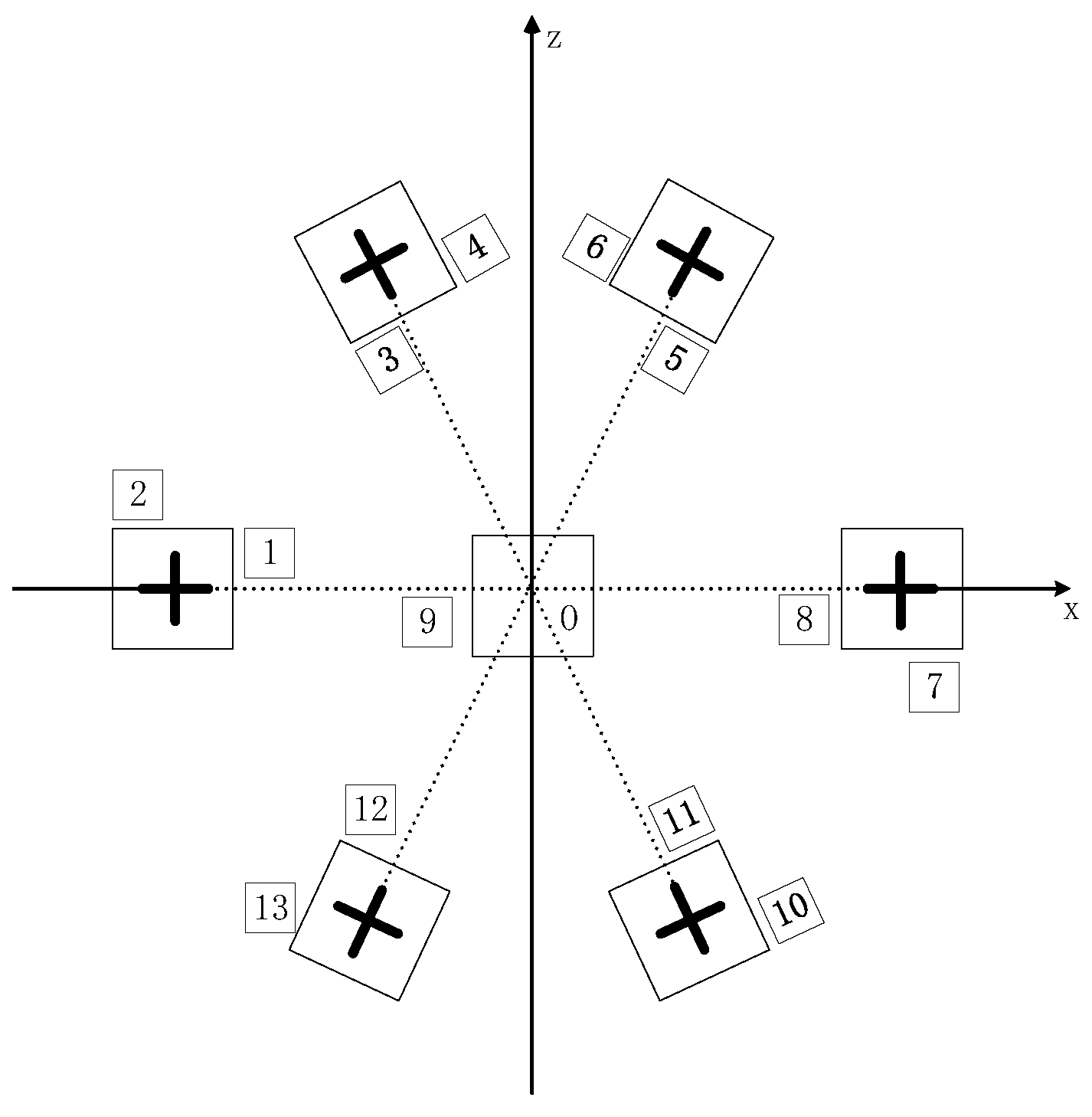
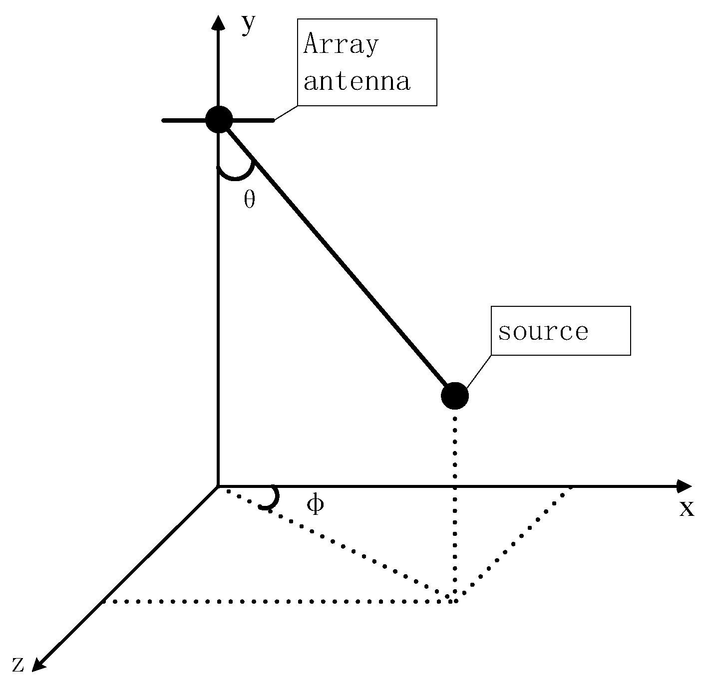
The schematic diagram of a circular antenna array is presented in Figure 1. In Figure 1, the middle antenna 9 is used as a single frequency estimation antenna corresponding to one receiving channel. Because this antenna is not switched, the number of sampling points collected is sufficient. FFT can better estimate the frequency offset. The surrounding six pairs of orthogonally polarized antennas, which include a total of 12 arrays, are used as circular antennas connected to another receiving channel. The schematic diagram of the positions of the array antenna and source during the observation is presented in Figure 2. The specific algorithm is given below.

Suppose that $s(t)$ is an incident signal waveform, $f_0$ is the signal carrier frequency, ${\lambda }_0$ is the signal wavelength, $\theta$ is the incidence pitch angle, and $\phi$ is the incidence azimuth. A two-channel circular array antenna is adopted to receive the incident signal, and the switching time interval of the acquisition antenna is $T$. Then, the received echo signals of an alternating acquisition antenna and a single-channel antenna can be respectively expressed as:

$$x_n(t)=b\times p_n(\theta ,\phi ,\gamma ,\eta )s[t+(n-1)T-{\tau }_n(\theta ,\varphi )]e^{i2\pi (f_0+f_d)[t+(n-1)T-{\tau }_n(\theta ,\varphi )]}$$

(1)

$$x_{n0}(t)=b\times p_0(\theta ,\phi ,\gamma ,\eta )s[t+(n-1)T-{\tau }_0(\theta ,\varphi )]e^{i2\pi (f_0+f_d)[t+(n-1)T-{\tau }_{n0}(\theta ,\varphi )]}$$

(2)

where $b$ represents the component related to the transmitting power of the source and the distance from the array antenna; $p_n(\theta ,\phi ,\gamma ,\eta )$ is the component related to the polarization; $\gamma$ and $\eta$ are two polarization parameters; ${\tau }_n(\theta ,\varphi )$ represents the time delay of the signal to the $n$ array element; $f_d$ is the Doppler frequency of the source.

After the frequency-mixing signal processing, the echo signals can be expressed as:

$$x_n(t)=b\times p_n(\theta ,\phi ,\gamma ,\eta )s[t]e^{-i2\pi f_0{\tau }_n(\theta ,\varphi )}{e}^{i2\pi f_d[t+(n-1)T-{\tau }_n(\theta ,\varphi )]}$$

(3)

$$x_{n0}(t)=b\times p_0(\theta ,\phi ,\gamma ,\eta )s[t]e^{-i2\pi f_0{\tau }_0(\theta ,\varphi )}{e}^{i2\pi f_d[t+(n-1)T-{\tau }_n(\theta ,\varphi )]}$$

(4)

The existence of the frequency synchronization error leads to the deviation between $\overline{f_0}$ and $f_0$, which can be expressed as $f_{\Delta }=f_0-\overline{f_0}$. Since a base station is generally arranged at a high level and the incident signals are narrowband signals in the far-field, the delay along the array of the envelope of the received signal can be ignored. Then, Equations (3) and (4) can be respectively rewritten as:

$$x_n(t)=b\times p_n(\theta ,\phi ,\gamma ,\eta )s[t]e^{-i2\pi f_0{\tau }_n(\theta ,\varphi )}{e}^{i2\pi (f_{\Delta }+f_d)[t+(n-1)T-{\tau }_n(\theta ,\varphi )]}$$

(5)

$$x_{n0}(t)=b\times p_0(\theta ,\phi ,\gamma ,\eta )s[t]e^{-i2\pi f_0{\tau }_0(\theta ,\varphi )}{e}^{i2\pi (f_{\Delta }+f_d)[t+(n-1)T-{\tau }_n(\theta ,\varphi )]}$$

(6)

For the $N$-point FFT transformation of $x_{n0}(t)$ the spectrum is expressed as follows:

$$X_N(k)=FFT[x_{n0}(t)]={\displaystyle \sum _{n=0}^{N-1}{x}_{n0}(t)e^{-j\frac{2\pi kn}{N}}}$$

(7)

where the spectrum line corresponding to the amplitude is $k$.

For the maximum value of the spectrum, the corresponding spectrum line is denoted as $k_1$. According to the maximum likelihood estimation principle, the relationship between the frequency offset value and $k_1$ can be obtained as follows:

$$f_{\Delta }=\{\begin{array}{cc}\frac{k1}{TN}& 0\le k1\le \frac{N}{2}-1\\ -\frac{N-k1}{TN}& \frac{N}{2}\le k1\le N-1\end{array}$$

(8)

According to Equation (8), the estimation accuracy of the frequency offset is directly related to the FFT length, and its maximum estimation error is obtained as $\frac{k1}{2TN}$. In this system, the data acquisition points of channel 2 are equal to the sum of the data acquisition points of 12 antennas in channel 1, so the FFT length is long enough to estimate the frequency offset accurately.

By substituting the estimated frequency offset value into Equation (5), the $2N$ matrix metadata arranged into a column vector can be obtained as follows:

$${\mathit{x}}_l=\left[\begin{array}{c}{x}_1(t_l)\\ x_2(t_l)\\ \\ x_{2N}(t_l)\end{array}\right]=b_l\times \mathit{p}(\theta ,\phi ,\gamma ,\eta )\odot {\mathit{a}}_s(\theta ,\phi )$$

(9)

where $\mathit{p}(\theta ,\phi ,\gamma ,\eta )=\mathit{P}(\theta ,\phi )\mathit{w}(\gamma ,\eta )$,$\mathit{P}(\theta ,\phi )=\left[\begin{array}{c}{\mathit{p}}_1^T(\theta ,\phi )\\ {\mathit{p}}_2^T(\theta ,\phi )\\ ⋮\\ {\mathit{p}}_{2N}^T(\theta ,\phi )\end{array}\right]$,$\mathit{w}(\gamma ,\eta )=\left[\begin{array}{c}\cos \gamma \\ \sin \gamma e^{i\eta }\end{array}\right]$, ${\mathit{a}}_s(\theta ,\varphi )=\left[\begin{array}{c}{e}^{-i2\pi f_0{\tau }_1(\theta ,\varphi )}{e}^{i2\pi (f_{\Delta }+f_d)[t+(n-1)T-{\tau }_1(\theta ,\varphi )]}\\ e^{-i2\pi f_0{\tau }_2(\theta ,\varphi )}{e}^{i2\pi (f_{\Delta }+f_d)[t+(n-1)T-{\tau }_2(\theta ,\varphi )]}\\ ⋮\\ e^{-i2\pi f_{2N}{\tau }_1(\theta ,\varphi )}{e}^{i2\pi (f_{\Delta }+f_d)[t+(n-1)T-{\tau }_{2N}(\theta ,\varphi )]}\end{array}\right]$, and $\odot$ denotes the Hardmard product.

Considering the receiver noise, the echo signal vector can be expressed as follows:

$${\mathit{y}}_i=b\mathit{a}(\theta ,\varphi ,\gamma ,\eta )+{\mathit{n}}_i$$

(10)

where $\mathit{a}(\theta ,\varphi ,\gamma ,\eta )=\mathit{p}(\theta ,\varphi ,\gamma ,\eta )e\mathit{a}(\theta ,\varphi )$, and ${\mathit{n}}_i\in CN(0,{\mathit{R}}_n)$ is a complex Gaussian noise vector with a zero mean and a covariance matrix ${\mathit{R}}_n$.

In an indoor environment, signals received by the array contain not only direct waves but also multipath echoes that reached the array after being reflected by various obstacles such as walls, tables, and floors. After considering these factors, the receiver echo signal ${\mathit{y}}_i$ can be expressed in the following form:

$${\mathit{y}}_i=\mathit{A}{\mathit{s}}_i+{\mathit{n}}_i$$

(11)

where $\mathit{A}=\left[\begin{array}{cccc}\mathit{a}({\theta }_1,{\varphi }_1,{\gamma }_1,{\eta }_1)& \mathit{a}({\theta }_2,{\varphi }_2,{\gamma }_2,{\eta }_2)& L& \mathit{a}({\theta }_P,{\varphi }_P,{\gamma }_P,{\eta }_P)\end{array}\right]$ denotes the array manifold matrix, $P$ is the number of direct waves and multipath signals, and ${\mathit{s}}_i$ is the signal vector, which can be expressed as:

$${\mathit{s}}_i{=[\mathrm{b}}_{1l}{,\mathrm{b}}_{2l}{,\mathrm{L},\mathrm{b}}_{Pl}{]}^T$$

(12)

In a multipath environment, the direct wave signal and multipath signal need to be separated to estimate the target direction accurately. In this case, a super-resolution angle estimation method is needed. Considering that the Multiple Signal Classificaion (MUSIC) spectrum estimation algorithm has the advantages of a small amount of computation and low complexity, the MUSIC spectrum estimation algorithm is adopted.

Assume that ${\widehat{\mathit{R}}}_{music}=\frac{1}{L}{\displaystyle \sum _{l=1}^L{\mathit{y}}_i{\mathit{y}}_i^H}$ is the covariance matrix of the received signal.

The spatial spectrum obtained by the MUSIC spectrum algorithm is expressed as follows:

$$Pmusic(\theta ,\varphi ,\gamma ,\eta )=\frac{1}{{\mathit{a}}^H(\theta ,\varphi ,\gamma ,\eta ){\mathit{Q}}_{music}\mathit{a}(\theta ,\varphi ,\gamma ,\eta )}$$

(13)

where ${\mathit{Q}}_{music}={\mathit{U}}_N{\mathit{U}}_N^H$, and ${\mathit{U}}_N$ is the eigenvector matrix of noise subspace derived from ${\widehat{\mathit{R}}}_{music}$ eigen decomposition.

The target parameter is obtained by searching the peak value of the spectral function by parameters, which can be expressed as:

$$[\widehat{\theta },\widehat{\phi },\widehat{\gamma },\widehat{\eta }]=\arg \max Pmusic(\theta ,\varphi ,\gamma ,\eta )$$

(14)

Since the above process is a four-dimensional search and requires a large amount of calculation, to reduce the amount of calculation, B is expressed in the following form by combining Equation (14) and the properties of the Hardmard product:

$$\mathit{a}(\theta ,\varphi ,\gamma ,\eta )=\mathit{p}(\theta ,\varphi ,\gamma ,\eta )e\mathit{a}(\theta ,\varphi )={\mathit{\Lambda }}_s(\theta ,\varphi )\mathit{P}(\theta ,\varphi )\mathit{\omega }(\gamma ,\eta )$$

(15)

where ${\mathit{\Lambda }}_s(\theta ,\varphi )$ denotes a diagonal matrix consisting of $\mathit{a}(\theta ,\varphi )$, so $Pmusic(\theta ,\varphi ,\gamma ,\eta )$ can be expressed as follows:

$$\begin{array}{ll}Pmusic(\theta ,\varphi ,\gamma ,\eta )& =\frac{1}{{\mathit{\omega }}^H(\gamma ,\eta ){\mathit{P}}^H(\theta ,\varphi ){\mathit{\Lambda }}_s^H(\theta ,\varphi ){\mathit{Q}}_{music}{\mathit{\Lambda }}_s(\theta ,\varphi )\mathit{P}(\theta ,\varphi )\mathit{\omega }(\gamma ,\eta )}\\ & =\frac{1}{{\mathit{\omega }}^H(\gamma ,\eta )\mathit{D}(\theta ,\varphi )\mathit{\omega }(\gamma ,\eta )}\end{array}$$

(16)

where $\mathit{D}(\theta ,\varphi )={\mathit{P}}^H(\theta ,\varphi ){\mathit{\Lambda }}_s^H(\theta ,\varphi ){\mathit{Q}}_{music}{\mathit{\Lambda }}_s(\theta ,\varphi )\mathit{P}(\theta ,\varphi )$.

To maximize $Pmusic(\theta ,\varphi ,\gamma ,\eta )$, $\mathit{D}(\theta ,\varphi )$ should be as small as possible, and parameter search can be achieved as follows:

$$[\hat{\theta },\hat{\phi }]=\arg \min {\lambda }_{\min }(\mathit{D}(\theta ,\varphi ))$$

(17)

where ${\lambda }_{\min }(\mathit{D}(\theta ,\varphi ))$ represents the minimum eigenvalue of $\mathit{D}(\theta ,\varphi )$.

Assuming that the vertical distance between the source and base station is $h$, the coordinates of the source location can be obtained by combining Figure 2 as follows:

$$[x,z]=[h\tan \theta \cos \phi ,h\tan \theta \sin \phi ]$$

(18)

3. Proposed Tracking Algorithm

According to Equation (7), the multipath and other factors in the echo signal of the receiver cannot be eliminated, and the characteristics of the reflected signals vary with the material and size of obstacles. Therefore, in an NLOS environment, the dynamic positioning accuracy of the proposed Bluetooth array angular measurement and positioning system decreases sharply. Therefore, if only relying on the positioning accuracy of the system, the high-precision positioning within the coverage area cannot be guaranteed, so the tracking algorithm is particularly important. After comparative analysis, this paper selects strong tracking kalman filtering algorithm as a basic tracking algorithm and optimizes it.

3.1. Strong Tracking Kalman Filter

The source coordinates and their rate of change are taken as the state parameters, ${\mathit{X}}_{cv,k}=\left[\begin{array}{cccc}{x}_k& z_k& v_x& v_z\end{array}\right]$.

Assume that the state equation is given by:

$${\mathit{X}}_{cv,k}=\mathit{F}{\mathit{X}}_{cv,k-1}+w_{cv,k}$$

(19)

where $\mathit{F}=\left[\begin{array}{cccc}1& 0& \Delta T& 0\\ 0& 1& 0& \Delta T\\ 0& 0& 1& 0\\ 0& 0& 0& 1\end{array}\right]$, $\Delta T$ is the data output interval expressed in seconds, and $w_{cv,k}$ is the system noise at the current moment, whose covariance matrix is ${\mathit{Q}}_{cv,k}$.

The measurement information represents directly output positioning information, so the measurement equation is given by:

$${\mathit{Z}}_{cv,k}=\mathit{H}{\mathit{X}}_{cv,k}+{\mathit{V}}_{cv,k}$$

(20)

where ${\mathit{Z}}_{cv,k}=\left[\begin{array}{cc}{x}_k^R& z_k^R\end{array}\right]$, ${\mathit{H}}_{cv,k}=\left[\begin{array}{cccc}1& 1& 0& 0\end{array}\right]$, $x_k^R$ is directly output location information at the current time; ${\mathit{V}}_{cv,k}$ is the measurement noise at the current moment, and its covariance matrix is ${\mathit{R}}_{cv,k}$.

In the strong tracking kalman filter, the gain matrix ${\mathit{K}}_k$ needs to be determined online to satisfy the following conditions:

$$E[x_k-{\hat{x}}_k]{[x_k-{\hat{x}}_k]}^T=\min$$

(21)

$$\begin{array}{cc}E[{\mathit{r}}_k^T{\mathit{r}}_{k+j}]=0,& k=0,1,2,\cdots ,j=1,2\cdots \end{array}$$

(22)

where ${\mathit{r}}_k={\mathit{Z}}_k-{\mathit{H}}_k{\mathit{X}}_{k,k-1}$ represents an innovation vector, whose covariance matrix is ${\mathit{N}}_k={\mathit{H}}_k{\mathit{P}}_{k,k-1}{\mathit{H}}_k^T$. Equation (22) requires ${\mathit{r}}_k$ to be orthogonal, which actually represents an index of the residual sequence that is orthogonal on the basis of the index of minimum variance of the residual.

If the signal is not affected by environmental factors, such as refraction, reflection, and multipath effect, it can be considered that ${\mathit{r}}_k$ obeys the Gaussian distribution with the zero mean. In this case, Equation (22) satisfies. Therefore, in that case, the strong tracking kalman filter represents the standard extended kalman filter. However, uncertain influencing factors in the external environment will lead to the deviation of the filter state estimate from the system state. In this situation, to realize the system state tracking by the filter, the gain matrix needs to be adjusted online to make the residual sequence still be mutually orthogonal.

Based on Equations (19) and (20), the strong tracking filtering algorithm can be expressed as follows:

$$\{\begin{array}{l}{X}_{k,k-1}=F{X}_{k-1}\\ P_{k,k-1}=L(k)F{P}_{k-1}{F}^T+Q_{cv,k-1}\\ K_k=P_{k,k-1}{H}_k^T{(H_k{P}_{k,k-1}{H}_k^T+R_{cv,k})}^{-1}\\ P_k=(I-K_k{H}_k)P_{k,k-1}\\ X_k=X_{k,k-1}+K_k(Z_k-H_k{X}_{k,k-1})\\ L(k)=diag[{\lambda }_{1(k)},{\lambda }_{2(k)},\cdots {\lambda }_{n(k)}]\end{array}$$

(23)

where ${\mathit{X}}_{k,k-1}$ is the predicted state vector, ${\mathit{P}}_{k,k-1}$ is the covariance matrix of the predicted state, ${\mathit{K}}_k$ is the Kalman gain matrix; ${\mathit{X}}_{k-1}$ and ${\mathit{X}}_k$ represent the estimated state matrices at times (k−1) and k, and ${\mathit{P}}_{k-1}$ and ${\mathit{P}}_k$ are their respective covariance matrices, respectively; $Z_k$ indicates the measured value at the current time; $\mathit{I}$ is the identity matrix; $L(k)$ is the time-varying elimination matrix; ${\lambda }_{i(k)}\ge 1(i=1,2,\cdots ,n)$ is the $n$ time-varying fading factor, which can be expressed as follows:

$${\lambda }_{i(k)}=\{\begin{array}{cc}{\lambda }_{0(k)}& {\lambda }_{0(k)}>1\\ 1& {\lambda }_{0(k)}\le 1\end{array}$$

(24)

where ${\lambda }_{0(k)}=\frac{Tr(N_k)}{Tr(M_k)}$, $V_{0,k}=\{\begin{array}{cc}{r}_0{r}_0^T& k=0\\ \frac{\rho V_{0,k-1}+r_k{r}_k^T}{1+\rho }& k\ge 1\end{array}$, $N_k=V_{0,k}-H_k{Q}_{k-1}{H}_k^T-l_k{R}_k$, and $\rho$ is the forgetting factor.

It can be seen that when the system state mutates, the increase in $V_{0,k}$ will increase with the $r_0{r}_0^T$, so the time-varying fading factor will also increase, and the tracking ability of the filter will be enhanced.

3.2. Improved Tracking Algorithm

It is considered that the covariance matrix $P_{k,k-1}$ is a symmetric matrix of the $n$th order. However, after enough large number of times of calculation, it no longer has non-negative and positive character. Suppose the rank is $e$, $0<e<1$, $S$ is a diagonal matrix, and they satisfy the semi-positive definite condition, whose eigenvalue is set as $\begin{array}{cccc}{\sigma }_1^2,& {\sigma }_2^2,& \cdots ,& {\sigma }_n^2\end{array}$, and it holds that ${\sigma }_1^2\ge {\sigma }_2^2\ge \cdots \ge {\sigma }_n^2,{\sigma }_{r+1}^2=\cdots ={\sigma }_n^2=0$. Then, there must be an orthogonal matrix $V$ of order $n$, making $P^{T}P$ similar to a diagonal matrix, which can be expressed as follows [34]:

$$V^T({P_{k,k-1}}^T{P}_{k,k-1})V=diag(\begin{array}{cccc}{\sigma }_1^2,& {\sigma }_2^2,& \cdots ,& {\sigma }_r^2,\end{array}\begin{array}{ccc}0,& \cdots ,& 0\end{array})=S_n^2=\left[\begin{array}{cc}{S}_r^2& 0\\ 0& 0\end{array}\right]$$

(25)

where $V=\left[\begin{array}{cc}{V}_1& V_2\end{array}\right]=[\begin{array}{cccc}{v}_1,& v_2,& \cdots ,& v_n\end{array}]$, and $P_{k,k-1}{V}_2=0$.

Set $U_1=P_{k,k-1}{V}_1{S}_r^{-1}$ to obtain $U_1^T{U}_1=I$, so the -column vectors of $U_1$ are unit orthonormal vectors, which can be extended to an orthonormal basis. There exists $U_2$ such that $U=[\begin{array}{cc}{U}_1& U_2\end{array}]$ is an orthonormal matrix of order $n$, and:

$$U^T{P}_{k,k-1}V=\left[\begin{array}{cc}{U}_1^T{P}_{k,k-1}{V}_1& U_1^T{P}_{k,k-1}{V}_2\\ U_2^T{P}_{k,k-1}{V}_1& U_1^T{P}_{k,k-1}{V}_2\end{array}\right]$$

(26)

From $U_1=P_{k,k-1}{V}_1{S}_r^{-1}$, we get $P_{k,k-1}{V}_1=U_1{S}_r$, which yields to:

$$U_1^T{P}_{k,k-1}{V}_1=S_r^{-1}{V}_1^T{P_{k,k-1}}^T{P}_{k,k-1}{V}_1=S_r^{-1}{S}_r^2=S_r$$

(27)

$$U_2^T{P}_{k,k-1}{V}_1=U_2^T{U}_1{S}_r=0$$

(28)

Further, because $P_{k,k-1}{V}_2=0$, then $U_1^T{P}_{k,k-1}{V}_2=U_2^T{P}_{k,k-1}{V}_2=0$.

$U^T{P}_{k,k-1}V=\left[\begin{array}{cc}I& 0\\ 0& 0\end{array}\right],P_{k,k-1}=U\left[\begin{array}{cc}I& 0\\ 0& 0\end{array}\right]V^T$.

Since is symmetric, it holds that:

$$\begin{array}{l}{V}^T({P_{k,k-1}}^T{P}_{k,k-1})V=V^T(P_{k,k-1}{P}_{k,k-1})V\\ =V^T(U{S}_n{V}^{T}U{S}_n{V}^T)V=(V^{T}U)S_n(V^{T}U)S_n=S_n^2\end{array}$$

(29)

So, $V^{T}U=I$ and $V=U$, which yields to:

$$P_{k,k-1}=U\left[\begin{array}{cc}{S}_r& 0\\ 0& 0\end{array}\right]U^T$$

(30)

By setting $D=\left[\begin{array}{cc}{S}_r& 0\\ 0& 0\end{array}\right]$, we obtain:

$$K_k=UD{U}^T{H}_k^T{(H_{k}UD{U}^T{H}_k^T+R_{cv,k})}^{-1}$$

(31)

The SVD is applicable to any matrix decomposition. It can express a complex matrix by the product of several relatively simple matrices (eigenvalues and eigenvectors), which can not only simplify the operation but also preserve the properties of the original matrix. In the classical kalman filter (KF) algorithm, the rounding error of the state covariance matrix gradually accumulates over time, leading to the loss of its non-negative property. Using the SVD can ensure its non-negative positive property so that the algorithm can go on and improve the operation accuracy.

In the Kalman filter, $r_k=Z_k-H_k{X}_{k,k-1}$ represents the innovation vector, and its covariance matrix is $N_k=H_k{P}_{k,k-1}{H}_k^T$. If the signal is not affected by environmental factors, such as refraction, reflection, and multipath effect, it can be considered that ${\mathit{r}}_k$ obeys the Gaussian distribution with the zero mean. If the influence of the external environmental factors leads to the decrease in the positioning accuracy or abnormal positioning values, it can be considered that ${\mathit{r}}_k$ follows the Gaussian distribution with the mean value of ${\mathit{Z}}_k-{\mathit{Z}}_k^T$, where ${\mathit{Z}}_k^T$ is the actual location. Based on the innovation vector and its covariance matrix, the test information is constructed as $\Delta r_k=r_k^T{D}^{-1}{r}_k$, and it is used as a condition to judge whether the positioning result is abnormal; it is defined as follows:

$$\{\begin{array}{cc}|\Delta r_k|\le m& \mathrm{Locate} \mathrm{normal}\\ |\Delta r_k|>m& \mathrm{Locate} \mathrm{abnormal}\end{array}$$

(32)

where $m$ denotes the threshold value, which is determined through multiple static tests at different points.

Huber functions are used to construct adaptive factors as follows:

$${\alpha }_k\{\begin{array}{cc}1& |\Delta {\mathit{r}}_k|\le m\\ \frac{\Delta {\mathit{r}}_k}{m}& |\Delta {\mathit{r}}_k|>m\end{array}$$

(33)

The robust estimation of positioning can be achieved by replacing $R_{cv,k}$ in the gain matrix with ${\alpha }_k{R}_{cv,k}$. The absolute value of $\Delta r$ is compared with the prior threshold information. When the absolute value of $\Delta r$ is greater than the prior threshold, the positioning result is considered abnormal. In this case, the robust factor of the constructed measurement noise is used to update its covariance matrix to achieve robust filtering performance and to improve the positioning accuracy.

The Sage–Husa filter can estimate and modify the statistical characteristics of the system noise in real-time so as to improve the filter accuracy further and has a certain anti-interference ability. Therefore, combined with the improved Sage–Husa filter, the covariance matrix of the system noise can be estimated in real-time as follows [24]:

$$\begin{array}{l}{\mathit{Q}}_{cv,k}=\left(1-{\beta }_k\right){\mathit{Q}}_{cv,k-1}+{\beta }_k[K_k{r}_k{r}_k^T{K}_k^T+P_k-F_{k-1}{P}_{k-1}{F}_{k-1}^T-\\ 2K_k{H}_k{P}_{k,k-1}{H}_k^T{K}_k^T-2K_k{\alpha }_k{R}_{cv,k}{K}_k^T+P_{k,k-1}{H}_k^T{K}_k^T+K_k{H}_k{P}_{k,k-1}]\end{array}$$

(34)

where ${\beta }_k=(1-b)/(1-b^{k+1})$, and $b$ is the forgetting factor, and $0<b<1$. In the updating process of ${\mathit{Q}}_{cv,k}$, to prevent losing the non-negativity characteristic of the matrix, the diagonal elements in the second part on the right side of Equation (34) are treated with absolute value, and the non-diagonal elements are treated with zero.

When calculating the predicted state covariance matrix, the improved Sage–Husa filtering is used for the system noise covariance matrix for continuous real-time estimation and correction. To reduce the state estimation error, the adaptive differential resistance factor, combined with the measurement noise covariance matrix, is updated, thus further improving the accuracy and obtaining more accurate location information.

Based on the above theories, the specific algorithm of SVD-STKF can be described as:

(1)

Calculate the one-step state prediction value according to Equation (19).

(2)

Calculate innovation vector according to $r_k=Z_k-H_k{X}_{k,k-1}$.

(3)

Calculate the prediction error covariance matrix according to Equation (23).

(4)

Calculate the SVD factorization of $P_{k,k-1}$.

(5)

Calculate Kalman gain matrix according to Equation (31).

(6)

Status updates according to Equation (23).

(7)

Test information is constructed based on innovation vector and its covariance matrix according to Equation (32).

(8)

Huber function is used to construct adaptive factors according to Equation (33).

(9)

Update error covariance matrix according to Equation (23).

4. Experimental Validation

4.1. Experimental Environment

The field diagram of the antenna array AOA positioning test is presented in Figure 3. The test was performed in a room which was 7 m long and 6 m wide. The passive antenna array was placed on the ceiling, and its axes were as shown Figure 1. The source used in this test was a tag that transmitted the Bluetooth signal.

The hardware of the array antenna and source is shown in Figure 4. The receiver collected data from the peripheral circle of the polarized antenna in a time-sharing manner, and the collection sequence was (1–2, 3–4, 5–6, 7–8, 10–11, 12–13). The number of collection cycles was two, and eight data points were collected at each time. The data collected by antenna No. 9 in the middle, which was the frequency estimation antenna, entered the receiver through another channel. The source uses a tag that emits Bluetooth signals.

The Bluetooth array AOA position was determined by measuring the source emission signal, realizing the signal arrive angle positioning. The accuracy of frequency estimation has a significant influence on positioning accuracy; therefore, in the test, the Bluetooth tag antenna used an omnidirectional antenna. However, in the actual environment, the source is placed in a different direction so that the positioning result can have a certain degree of difference. Under the condition of different source locations, positioning accuracy was different. The farther the distance between the source and the base station, the lower the positioning accuracy. To verify the validity of the proposed algorithm, the static test, rotation test, and dynamic test were conducted on the source. It was assumed that the height of the source was known, and the true height of the source was substituted into the positioning formula. The defined relative coordinate system had the origin right below the center of the antenna array. In the actual scene, the x-axis and z-axis point, as shown Figure 3, which is consistent with the direction in Figure 2. The height of the source was about 3.35 m. To reduce the calculation complexity, the search range was limited to the range of the array beamwidth. The simulation results based on Matlab were as follows.

4.2. Empirical Positioning Algorithm

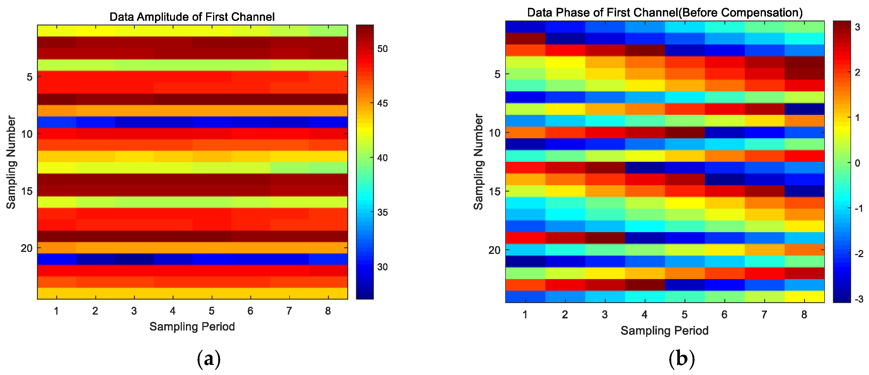
Figure 5 shows the single-frame data, including the amplitude and phase diagrams, where the horizontal axis denotes the sampling period, according to each antenna collection point, and the vertical axis represents the sampling sequence number in terms of the antenna number and order of calculating. Thus, for the single-channel data, although the amplitude of fundamental was not affected, the phase diagram was obviously affected by the presence of excess phase. The phase stability had a great influence on the accuracy and stability of subsequent positioning.

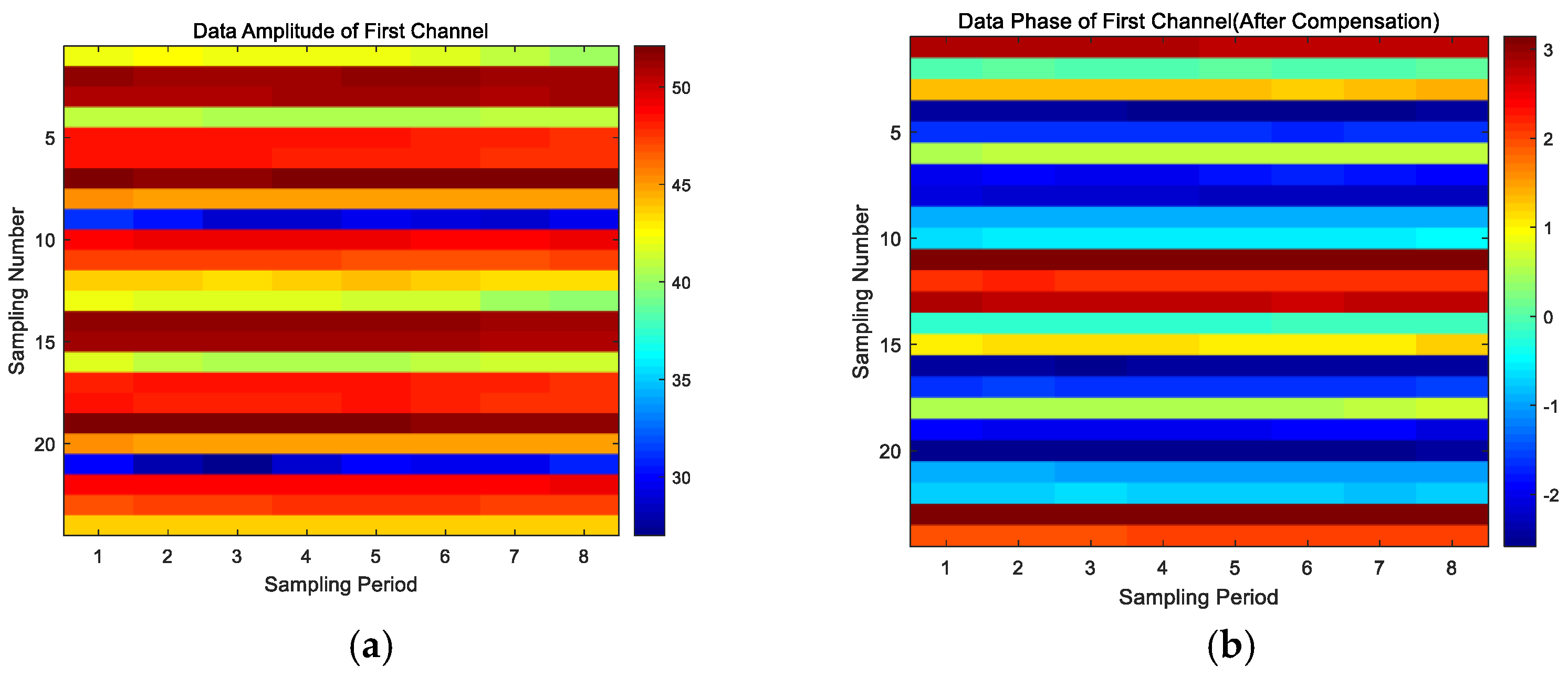
Figure 6 shows the amplitude and phase diagrams of the single-frame data after the compensation, where it can be seen that after the comparison, the redundant phase caused by the frequency deviation was complemented, and the redundant phase was corrected well.

To verify the effect of frequency estimation on the positioning results, the positioning results at the point (0, 0) with the compensation frequencies $\overline{f_0}$ and $\overline{f_0}\pm 2k$ are statistically analyzed in this paper. The estimated frequency at the point (0, 0) is 254 kHz.

Table 1. Influence of different frequencies on positioning results.

Point	Direction Component	Frequency (kHz)	Maximum Error (m)
(0, 0)	X	254	0.208
		256	0.415
		252	0.377
	Z	254	0.125
		256	0.269
		252	0.306

shows the positioning results. The statistical results show that a 2 kHz frequency estimation deviation can cause a 0.3 m positioning deviation. Therefore, the accuracy of the compensated frequency estimation is extremely important.

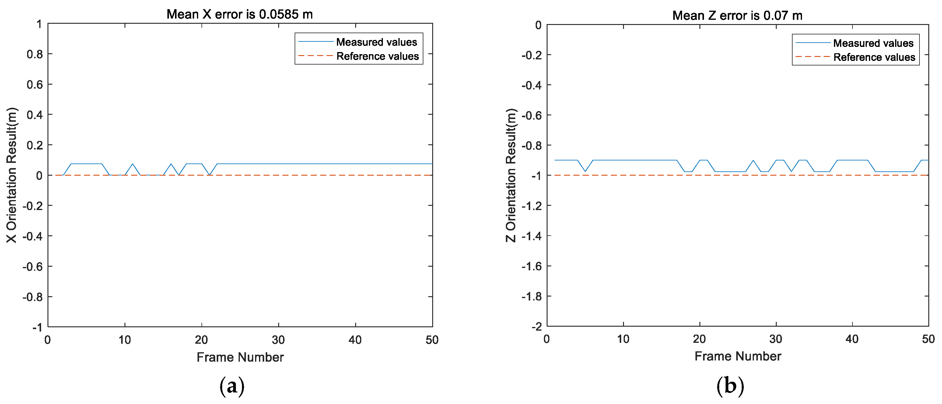
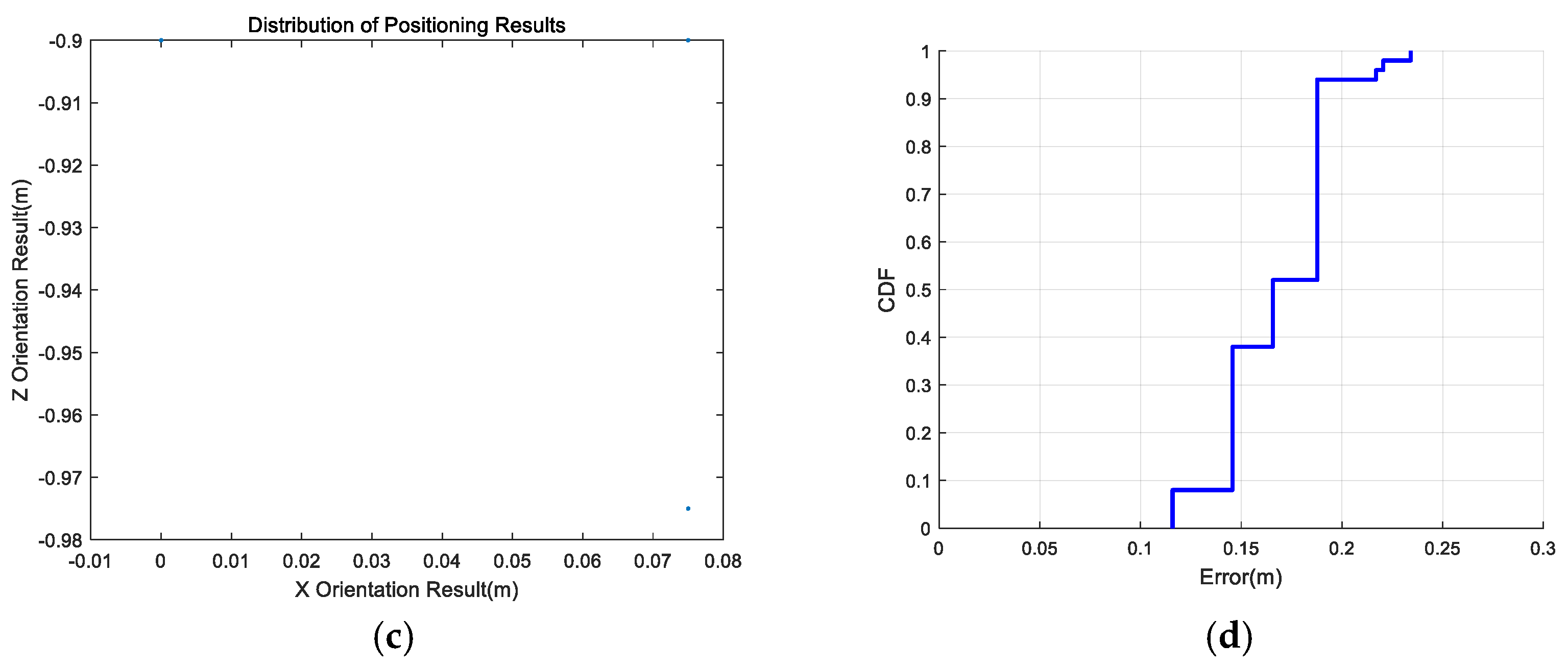
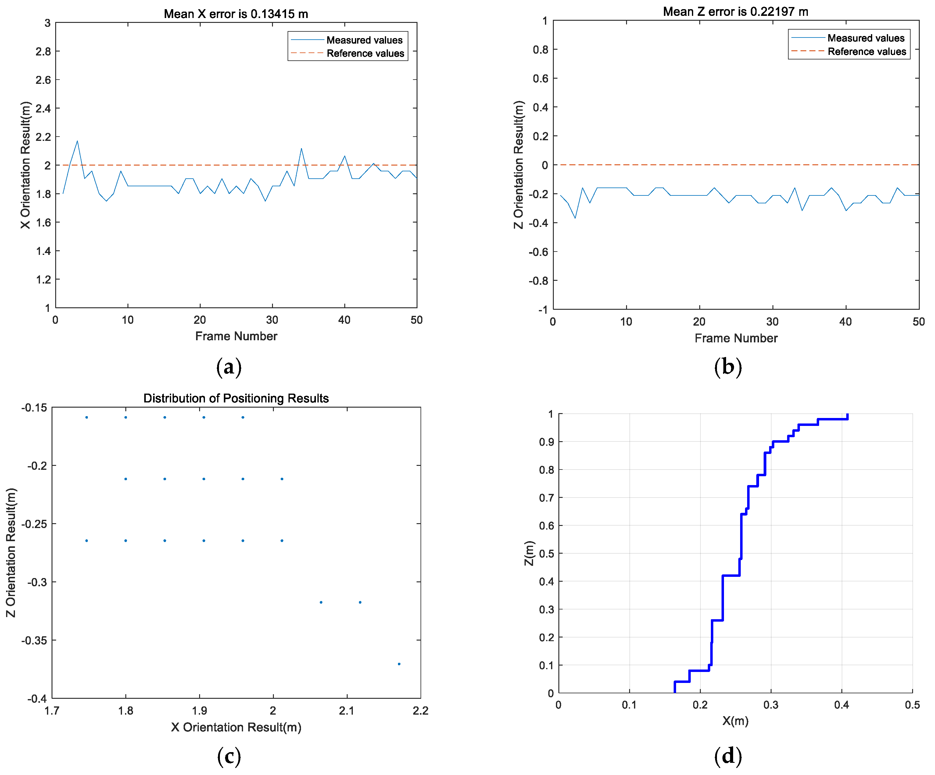
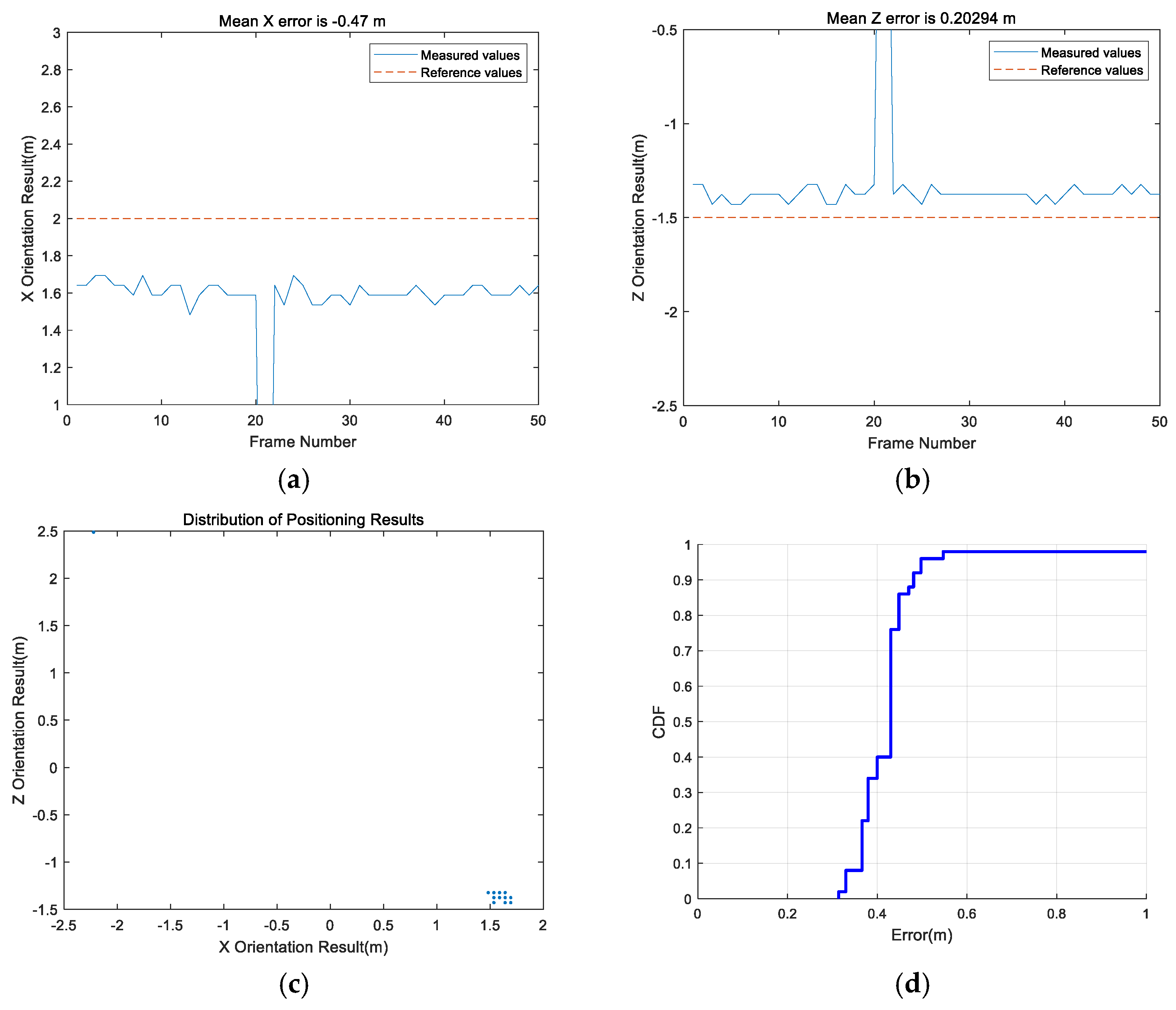
When the location of a source is different, the positioning accuracy is also different, so the static test was performed at different distances from the base station. In the static test, points (0, −1), (2, 0), and (2, −1.5) with different distances on the x-axis, z-axis, and non-coordinate axis were selected for testing. Fifty frames of data were collected at each position. The results are shown in Figure 7, Figure 8 and Figure 9. In the error graphs, the yellow horizontal line represents the coordinate value of the current position, the blue curve represents the positioning value given by the current system, the horizontal axis indicates the number of sampled frames, and the vertical axis represents the error value. In the distribution diagram of anchor points, the horizontal axis is x, the vertical axis is z, and the blue point represents the anchor point position of certain frame data. In the CDF diagrams, the horizontal axis represents the positioning error of the point, which can be calculated by $\sqrt{\Delta x^2+\Delta z^2}$, where $\Delta x$ and $\Delta z$ represent the errors of the current location point in the x- and z-directions, respectively, and the vertical axis represents the CDF. The multi-frame positioning results of the source at the point (0, −1) are shown in Figure 7, where it can be seen that the accuracies in the x-direction and z-direction were about 0.058 m and 0.07 m, respectively. The positioning results were good and stable without any jump point. As can be seen from the CDF diagram, the positioning errors were all within 0.3 m. The static test location results for the source locations of (2, 0) and (2, 1.5) are presented in Figure 8 and Figure 9, respectively, where it can be seen that the positioning accuracy was higher for the source location of (2, 0). The precision in the x-direction was about 0.1 m, whereas the accuracy in the z-direction of about 0.22 m. At point (2, 1.5), the source and array antenna elevation angle was close to 45°, so the accuracy was a little poor. However, there was only one peak point within 0.5 m, which could be interfered with by the other signals. The CDF diagram in Figure 8 and Figure 9 show that the positioning errors were within 0.5 m and 0.6 m, respectively.

4.3. Empirical Tracking Algorithm

4.3.1. Empirical Source Rotation Positioning

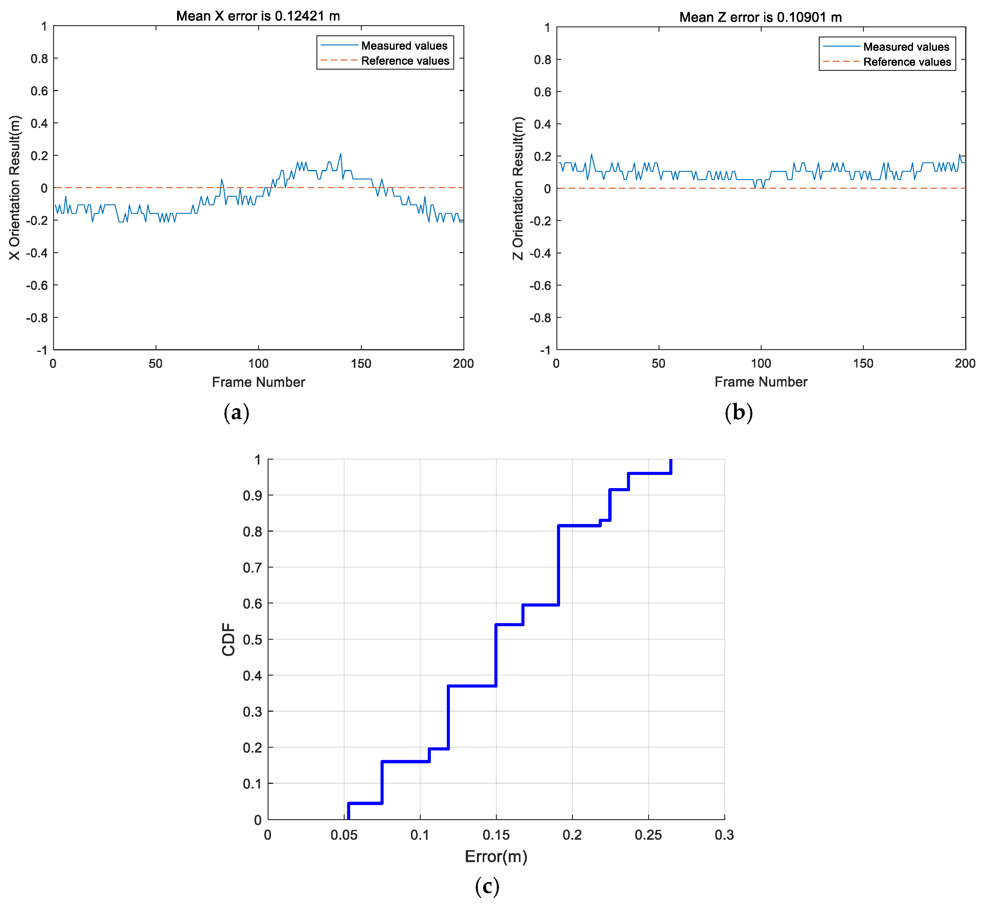
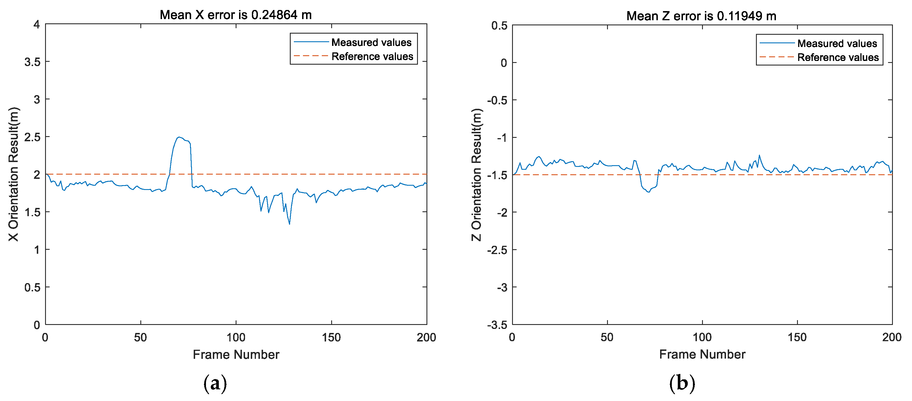
In the source rotation test, two representative points were used, point (0, 0) that was directly below the antenna, and point (2, −1.5) that was far away from the antenna on the non-coordinate axis. During the test, 200 frames of data were collected at each point. The error diagram of 200 frame data and the CDF graph corresponding to the single-frame data are presented in Figure 10 and Figure 11. In the error graph, the yellow horizontal line represents the coordinate value of the current position, the blue curve represents the positioning value obtained by the system, the horizontal axis is the number of sampled frames, and the vertical axis is the error value. In the CDF graph, the horizontal axis represents positioning error of this point, the vertical axis represents CDF. The precision in x-direction was about 0.124 m, and that in z-direction was about 0.109 m. The positioning result was good, and there was no jump point. It can be seen from the CDF diagram that the positioning errors are all within 0.3 m. The positioning result in the x-direction was strongly affected by the source rotation, which showed a trend of first decreasing, then increasing, and finally, decreasing. The positioning results in the z-direction were stable under the source rotation. Since point (2, −1.5) was far away from the base station, its positioning error increases. The precision in the x-direction was about 0.255 m, and that in the z-direction was about 0.125 m. Thus, when the source was far away from the base station, the positioning accuracy of some frames fluctuated significantly, with the maximum value exceeding 0.5 m. The CDF diagram shows that the positioning errors are all within 0.8 m.

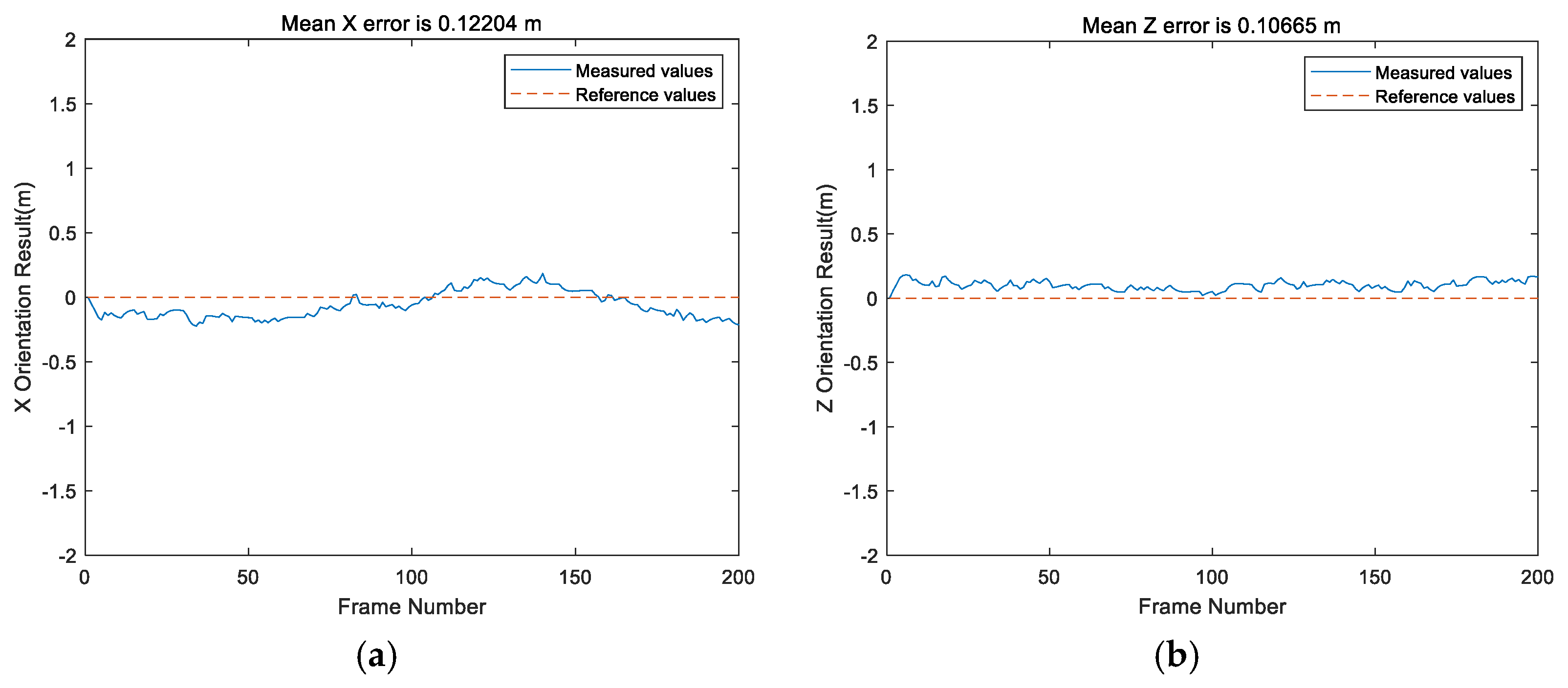
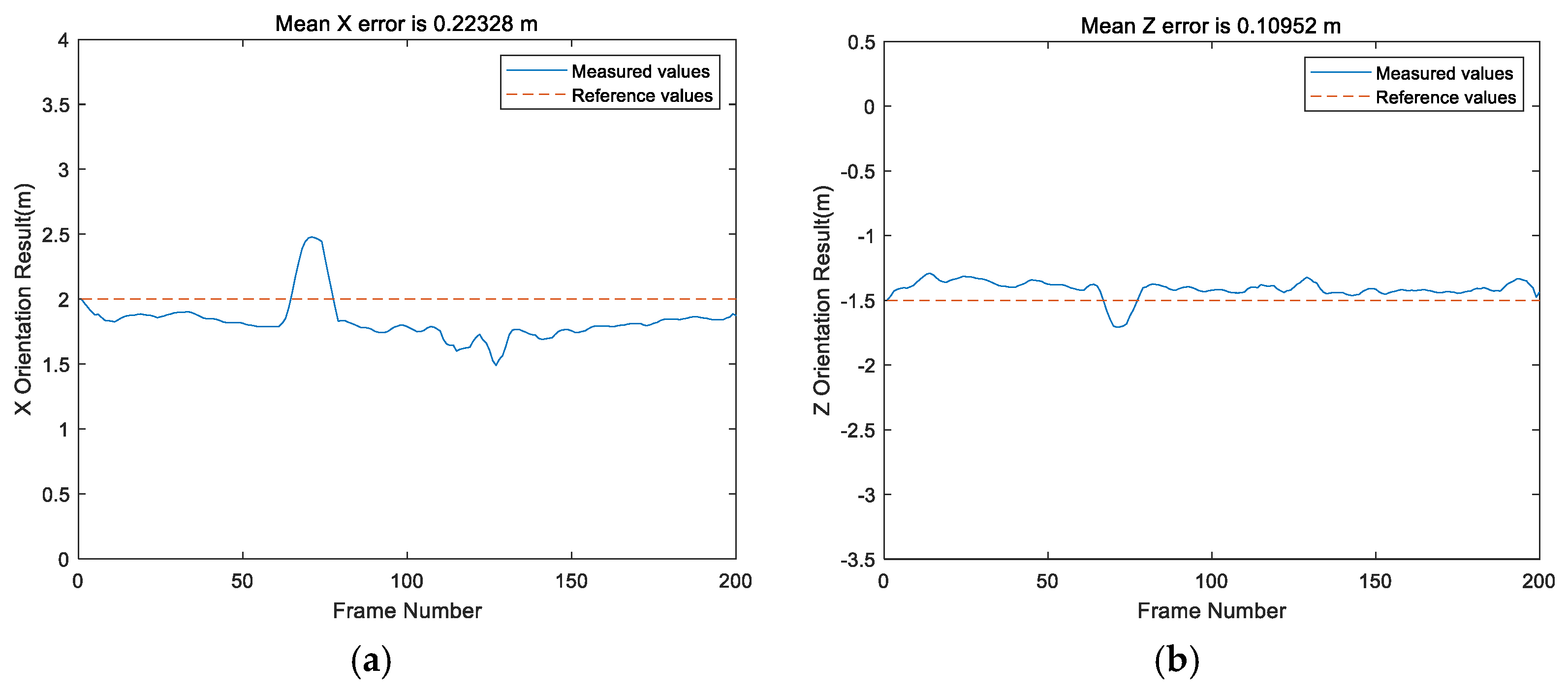
In addition, the STKF was applied to the above two points. The positioning results after the STKF optimization are shown in Figure 12 and Figure 13. The positioning accuracy of the point (0, 0) in the x-direction was about 0.122 m, and that in the y-direction was about 0.106 m. Compared with the results before the optimization, the accuracies in the x- and y-directions were improved by approximately 0.002 m and 0.003 m, respectively. The positioning accuracies of the point (2, −1.5) in the x- and z-directions were approximately 0.239 m and 0.119 m, respectively. Compared with the results before the optimization, the positioning accuracies in the x- and z-directions were improved by approximately 0.006 m and 0.005 m, respectively. Due to the instability of the positioning result caused by the source rotation, the STKF could only slightly improve the positioning accuracy; the accuracy improvement was small, by only a few millimeters. The positioning result was smoother than before the modification, but there was no significant correction for the mutation of point (2, −1.5).

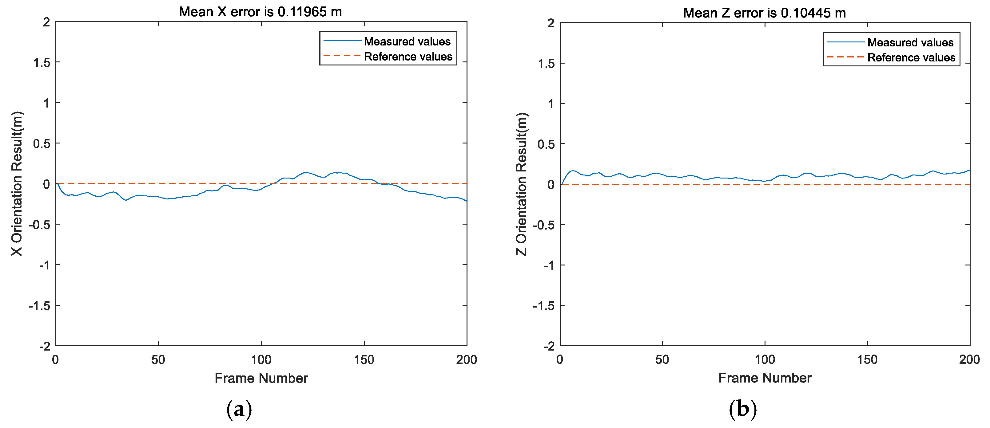
As shown in Figure 14 and Figure 15, in the case of source rotation, the strong tracking kalman filter could make the positioning result smoother, but the accuracy improvement was small. The singular value decomposition strong tracking kalman filter (SVD-STKF) was performed for the above two points. The positioning results after the SVD-STKF optimization are shown in Figure 9 and Figure 10. The positioning accuracies of the point (0, 0) in the x- and y-direction were approximately 0.12 m and 0.104 m, respectively. Compared with the results before the optimization, the accuracies in the x- and y-direction were improved by approximately 0.004 m and 0.003 m, respectively. The positioning accuracies of the point (2, −1.5) in the x- and z-direction were improved by approximately 0.226 m and 0.11 m, respectively. Compared with the results before the optimization, the positioning accuracies in the x- and z-direction were improved by about 0.029 m and 0.019 m, respectively. Compared with the STKF, the SVD-STKF achieved a more obvious improvement in accuracy and had a better tracking ability in the system mutation state. The accuracy of the mutation value at the point (2, −1.5) was improved by more than 0.05 m.

As shown in Figure 14 and Figure 15, for the point (0, 0), which was directly below the antenna, due to the strong signal, the positioning accuracy of the system was high, and the correction effect of the KF on it was not obvious. At this time, the difference between the SVD-STKF and strong KF tracking was small. However, for the distant point (2, −1.5), the stability of the signal decreased compared to the point (0, 0). Under the process of source rotation, the measurement error of some angles was large, and although the STKF improved the smoothness, the improvement in the accuracy was not obvious. The SVD-STKF provided a more obvious correction of the positioning results compared to the STKF. The overall positioning accuracy was improved by about 0.03 m, and the tracking ability for the abrupt state was stronger. The maximum error was reduced from 0.595 to 0.51, and the overall smoothing effect was good. The specific statistical results are given in

Table 2. Source rotation test error statistics.

Point	Direction Component	Filter Method	Maximum Error (m)	RMS
(0, 0)	x	Raw Output	0.21765	0.124
		STKF	0.215	0.122
		SVD-STKF	0.215	0.12
	z	Raw output	0.21765	0.109
		STKF	0.191	0.107
		SVD-STKF	0.189	0.104
(2,−1.5)	x	Raw output	0.541	0.255
		STKF	0.532	0.249
		SVD-STKF	0.47	0.223
	z	Raw output	0.247	0.125
		STKF	0.227	0.119
		SVD-STKF	0.204	0.11

.

To present the positioning results more intuitively, the distribution of anchor points is presented in Figure 16, where the horizontal axis represents the x-coordinate, and the vertical axis represents the z-coordinate. In Figure 16, the point represented by the red circle denotes the original output; the point represented by the blue asterisk denotes the output position obtained by the STKF; the point represented by the green plus sign denotes the output position of the SVD-STKF. As shown in Figure 16, after the STKF processing, the deviation degree between the anchor point and actual position decreased, and the accuracy of the maximum error point was improved to a certain extent, which was closer to the real position. The SVD-STKF showed the same effect, but the correction effect was better for the point position, especially for the mutation of the outliers.

4.3.2. Empirical Dynamic Positioning

In the case of source rotation, although the direction of the source had an impact on the positioning result, there was no occlusion in the signal propagation. Therefore, at the point (2, −1.5), which was far away from the base station, the maximum error value was 0.595 m, and the positioning accuracy could also be guaranteed within 1 m. However, for dynamic scenes, factors such as signal occlusion and multipath cannot be avoided in the process of moving pedestrians equipped with information sources. Therefore, dynamic positioning experiments were carried out, and the dynamic experiment process was as follows.

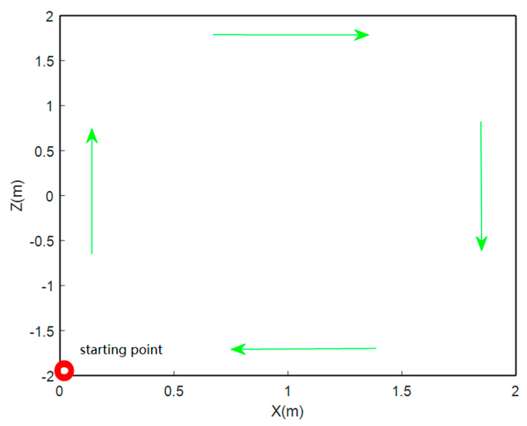
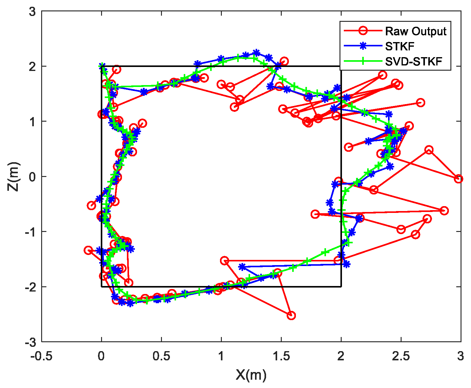
The user held the information source; the point (0, 2) was the starting point; the user traveled along the z-axis to the point (0, −2), then traveled along the positive direction of the x-axis to the point (2, −2), then turned to the positive direction of the z-axis to the point (2, 2), and finally, traveled along the negative direction of the x-axis to the starting point. The traveling diagram is presented in Figure 17, where the red circle indicates the starting position and green arrows indicate the direction of travel.

The trajectory comparison diagram after filtering is presented in Figure 18, where the horizontal axis represents the x-coordinate, and the vertical axis represents the z-coordinate; the point position represented by the red circle is the original output value, the blue asterisk represents the output value of the STKF algorithm, the green plus sign indicates the output value of the SVD-STKF algorithm, and the rectangle formed by the solid black line represents the true trajectory. As shown in Figure 18, in the process of normal pedestrian walking, the signal occlusion was not obvious when the pedestrian was walking along the z-axis, and the positioning effect was good. However, when the pedestrian was far away from the base station, due to the decrease in the positioning accuracy and severe signal occlusion, the positioning result had a large deviation. The offset of the farthest point from the real trajectory was close to 1 m, and the offset of the other anchor points was also large—almost all of them were above 0.5 m. The Hausdorff distance was 0.979 m. Therefore, in the dynamic process, due to the influences of signal occlusion and other factors, if the original output of the system is relied on, the positioning accuracy of distant points cannot be guaranteed. After the STKF correction, the trajectory was basically close to the real trajectory, the remote location points could be corrected, and the positioning results were smoother without random mutation points. The Hausdorff distance was increased to 0.519 m, achieving an increase of 0.46 m. On this basis, compared with the STKF algorithm, the SVD-STKF algorithm achieved more obvious corrections of the positioning results, making them be more close to the real trajectory; also, the Hausdorff distance was further increased to 0.464 m by 0.515 m.

5. Conclusions

In this paper, the static positioning accuracy, rotational positioning accuracy, and dynamic positioning accuracy in an NLOS environment are analyzed. The results show that in a line-of-sight (LOS) environment, the positioning accuracy of the Bluetooth array angle measurement is higher in its coverage range than in NLOS environment. The positioning accuracy of the points within 0.3 m (i.e., the near distance) can be guaranteed, but the maximum positioning error of points at a long distance can reach 0.595 m. The proposed SVD-STKF algorithm can improve the overall positioning accuracy up to 0.03 m, and the maximum value can be modified by 0.08 m. In the NLOS environment, the positioning accuracy decreases sharply, and the positioning error is close to 1 m in severe cases. However, the proposed SVD-STKF algorithm has a good effect. By using the proposed algorithm, the Hausdorff distance is improved by 0.513 m, the positioning results are smoother, there is no random mutation point, and good correction for the points far from the true trajectory is achieved. The comprehensive comparison results show that the proposed positioning algorithm can achieve the positioning accuracy within 1 m in the coverage area in a LOS environment, while in an NLOS environment, the dynamic positioning accuracy of the proposed Bluetooth array angular measurement and positioning system decreases sharply. Thus, by relying only on the positioning accuracy of the proposed system, the high-precision positioning within the coverage area cannot be guaranteed. However, after modifying the SVD-STKF tracking algorithm, the positioning accuracy within 1 m can be achieved for the source rotation situation in a LOS environment and the dynamic situation in an NLOS environment. Therefore, the high-precision positioning in the coverage area can be achieved by using a single base station.

References

1. Liu, J.; Chen, R.; Chen, Y.; Pei, L.; Chen, L. iParking: An Intelligent Indoor Location-Based Smartphone Parking Service. Sensors 2012, 12, 14612–14629. [Google Scholar] [CrossRef] [PubMed]
2. Wang, L.; Chen, R.; Shen, L.; Qiu, H.; Li, M.; Zhang, P.; Pan, Y. NLOS Mitigation in Sparse Anchor Environments with the Misclosure Check Algorithm. Remote Sens. 2019, 11, 773. [Google Scholar] [CrossRef] [Green Version]
3. Liu, Z.; Chen, R.; Ye, F.; Guo, G.; Li, Z.; Qian, L. Improved TOA Estimation Method for Acoustic Ranging in a Reverberant Environment. IEEE Sens. J. 2020. [Google Scholar] [CrossRef]
4. Xie, B.; Tan, G.; He, T. SpinLight: A High Accuracy and Robust Light Positioning System for Indoor Applications. In Proceedings of the 13th ACM Conference on Embedded Networked Sensor Systems, Seoul, Korea, 1–4 November 2015; pp. 211–223. [Google Scholar]
5. Chen, L.; Pei, L.; Kuusniemi, H.; Chen, Y.; Kröger, T.; Chen, R. Bayesian Fusion for Indoor Positioning Using Bluetooth Fingerprints. Wirel. Pers. Commun. 2013, 70, 1735–1745. [Google Scholar] [CrossRef]
6. Ye, F.; Chen, R.; Guo, G.; Peng, X.; Liu, Z.; Huang, L. A Low-Cost Single-Anchor Solution for Indoor Positioning Using BLE and Inertial Sensor Data. IEEE Access 2019, 7, 162439–162453. [Google Scholar] [CrossRef]
7. Yu, Y.; Chen, R.; Chen, L.; Guo, G.; Ye, F.; Liu, Z. A Robust Dead Reckoning Algorithm Based on Wi-Fi FTM and Multiple Sensors. Remote Sens. 2019, 11, 504. [Google Scholar] [CrossRef] [Green Version]
8. Guo, G.; Chen, R.; Ye, F.; Peng, X.; Liu, Z.; Pan, Y. Indoor Smartphone Localization: A Hybrid WiFi RTT-RSS Ranging Approach. IEEE Access 2019, 7, 176767–176781. [Google Scholar] [CrossRef]
9. Pengzhan, C.; Ye, K.; Xiaoyue, C. A UWB/Improved PDR Integration Algorithm Applied to Dynamic Indoor Positioning for Pedestrians. Sensors 2017, 17, 2065. [Google Scholar]
10. Kuang, J.; Niu, X.; Zhang, P.; Chen, X. Indoor Positioning Based on Pedestrian Dead Reckoning and Magnetic Field Matching for Smartphones. Sensors 2018, 18, 4142. [Google Scholar] [CrossRef] [Green Version]
11. Fan, Q.; Zhang, H.; Pan, P.; Zhuang, X.; Jia, J.; Zhang, P.; Zhao, Z.; Zhu, G.; Tang, Y. Improved Pedestrian Dead Reckoning Based on a Robust Adaptive Kalman Filter for Indoor Inertial Location System. Sensors 2019, 19, 294. [Google Scholar] [CrossRef] [PubMed] [Green Version]
12. Wang, B.; Gan, X.; Liu, X.; Yu, B.; Jia, R.; Huang, L.; Jia, H. A Novel Weighted KNN Algorithm Based on RSS Similarity and Position Distance for Wi-Fi Fingerprint Positioning. IEEE Access 2020, 8, 30591–30602. [Google Scholar] [CrossRef]
13. Ke, M.; Xu, Y.; Anpalagan, A.; Liu, D.; Zhang, Y. Distributed TOA-Based Positioning in Wireless Sensor Networks: A Potential Game Approach. IEEE Commun. Lett. 2017, 22, 316–319. [Google Scholar] [CrossRef]
14. Napoleon, S.A.; Omar, A.; Elramly, S.H.; Khamis, S.A.; Nasr, M.E. C5. Time difference of arrival by IEEE 802.11a, g based on practical estimation. In Proceedings of the 2012 29th National Radio Science Conference (NRSC), Cairo, Egypt, 10–12 April 2012; pp. 185–190. [Google Scholar]
15. Ruizhi, C.; Liang, C. Indoor positioning with smartphones: The state-of-the-art and the challenges. Acta Geod. Cartogr. Sin. 2017, 46, 118–128. [Google Scholar]
16. Zhang, R.; Hoflinger, F.; Reindl, L. Inertial sensor based indoor localization and monitoring system for emergency responders. IEEE Sens. J. 2013, 13, 838–848. [Google Scholar] [CrossRef]
17. Bluetooth Core Specification v5.1. Available online: https://www.bluetooth.com/events/launch-preview-bluetooth-core-specification-v5-1/ (accessed on 1 January 2019).
18. Zhen, J.; Wu, J.; Liu, J.; Xu, S.; Zhou, Z.; Xin, H. A High Accuracy Positioning Method for Single Base Station in Indoor Emergency Environment. Geomat. Inf. Sci. Wuhan Univ. 2020, 45, 1146–1154. [Google Scholar] [CrossRef]
19. Zhang, H.; Xie, J.; Ge, J.; Lu, W.; Liu, B. Strong tracking sckf based on adaptive cs model for maneuvering aircraft tracking. IET Radar Sonar Navigation 2018, 12, 742–749. [Google Scholar] [CrossRef]
20. Ma, Y.-F. Research on MSINS/GPS Integrated Navigation System and Its Data Fusion Technology; Southeast University: Nanjing, China, 2006. [Google Scholar]
21. Zhang, Q. Adaptive kalman filter for actuator fault diagnosis. IFAC-PapersOnLine 2017, 50, 14272–14277. [Google Scholar] [CrossRef]
22. Ding, W.; Wang, J.; Rizos, C. Improving Adaptive Kalman Estimation in GPS/INS Integration. J. Navig. 2007, 60, 517–529. [Google Scholar] [CrossRef] [Green Version]
23. Wei, W.; Qin, Y.Y.; Zhang, X.D.; Zhang, Y.C. Amelioration of the Sage Husa algorithm. J. Chin. Inert. Technol. 2012, 20, 678–686. [Google Scholar]
24. Sage, A.P.; Husa, G.W. Adaptive filtering with unknown prior statistics. Joint Autom. Control Conf. 1969, 760–769. [Google Scholar] [CrossRef]
25. Lichtfuse, E. Non-GPS Navigation Using Vision-Aiding and Active Radio Range Measurements; Department of the Air Force Air University, Air Force Institute of Technology, Wright-Pattersion Air Force Base: Greene County, OH, USA, 2011. [Google Scholar]
26. Hou, D.H.; Frank, P.M. Strong tracking filtering of nonlinear timevarying stochastic systems with coloured noise: Application to parameter estimation and empirical robustness analysis. Int. J. Control. 1996, 65, 295–307. [Google Scholar]
27. Hu, G.; Gao, S.; Zhong, Y.; Gao, B.; Subic, A. Modified strong tracking unscented Kalman filter for nonlinear state estimation with process model uncertainty. Int. J. Adapt. Control. Signal Process. 2015, 29, 1561–1577. [Google Scholar] [CrossRef]
28. Zhang, Y.; Li, X.; Yang, Z. On strong tracking Kalman filter based on forgetting factor dynamic optimization. In Proceedings of the 30th Chinese Control Conference, Yantai, China, 22–24 July 2011. [Google Scholar]
29. Chen, Y.; Li, W.; Xin, G.; Yang, H.; Xia, T. An Improved Strong Tracking Kalman Filter Algorithm for the Initial Alignment of the Shearer. Complexity 2019, 2019, 3172501. [Google Scholar] [CrossRef]
30. Jwo, D.J.; Wang, S.H. Adaptive Fuzzy Strong Tracking Extended Kalman Filtering for GPS Navigation. IEEE Sens. J. 2007, 7, 778–789. [Google Scholar] [CrossRef]
31. Wang, L.; Libert, G.; Minneback, P. A singular value decomposition based Kalman filter algorithm. In Proceedings of the 1992 International Conference on Industrial Electronics, Control, Instrumentation, and Automation, San Diego, CA, USA, 13 November 1992; Volume 3, pp. 1352–1357. [Google Scholar]
32. Kulikova, M.V.; Tsyganova, J.V. Improved discrete-time Kalman filtering within singular value decomposition. IET Control Theory Appl. 2017, 11, 2412–2418. [Google Scholar] [CrossRef] [Green Version]
33. Manneback, P. Kalman filter algorithm based on singular value decomposition. In Proceedings of the 31st IEEE Conference on Decision and Control, Tucson, AZ, USA, 16–18 December 1992. [Google Scholar]
34. Chun, M.A.; Zhang, Q.; Yang, W. Performance evaluation of cubature Kalman filter based on singular value decomposition. Sci. Surv. Mapp. 2018, 43, 23–27. [Google Scholar]
Figure 1. Circular array antenna illustration.
Remotesensing 13 04301 g001
Figure 2. Illustration of antenna.
Remotesensing 13 04301 g002
Figure 3. Test field image.
Remotesensing 13 04301 g003
Figure 4. The hardware of the array antenna and source.
Remotesensing 13 04301 g004
Figure 5. Amplitude and phase of the single–frame data. (a) Amplitude. (b) Phase.
Remotesensing 13 04301 g005
Figure 6. Amplitude and phase of the single–-frame data after compensation. (a) Amplitude after compensation. (b) Phase after compensation.
Remotesensing 13 04301 g006
Figure 7. The static test location results for the source location of (0, −1). (a) Average error in the x-direction. (b) Average error in the z-direction. (c) Location distribution. (d) CDF.
Remotesensing 13 04301 g007aRemotesensing 13 04301 g007b
Figure 8. The static test location results for the source location of (2, 0). (a) Average error in the x-direction. (b) Average error in the z-direction. (c) Location distribution. (d) CDF.
Remotesensing 13 04301 g008
Figure 9. The static test location results for the source location of (2, −1.5). (a) Average error in the x-direction. (b) Average error in the z-direction. (c) Location distribution. (d) CDF.
Remotesensing 13 04301 g009
Figure 10. The source rotation test positioning results at the point (0, 0). (a) Error in the x-direction. (b) Error in the z-direction. (c) CDF.
Remotesensing 13 04301 g010
Figure 11. The source rotation test positioning results at the point (2, −1.5). (a) Error in the x-direction. (b) Error in the z-direction. (c) CDF.
Remotesensing 13 04301 g011aRemotesensing 13 04301 g011b
Figure 12. The strong tracking kalman filter (STKF) positioning results under the source rotation for the point (0, 0). (a) Error in the x-direction. (b) Error in the z-direction.
Remotesensing 13 04301 g012
Figure 13. The STKF positioning results under the source rotation for the point (2, −1.5). (a) Error in the x-direction. (b) Error in the z-direction.
Remotesensing 13 04301 g013
Figure 14. The singular value decomposition SVD–STKF positioning results under the source rotation for the point (0, 0). (a) Error in the x-direction. (b) Error in the z-direction.
Remotesensing 13 04301 g014
Figure 15. The SVD–STKF positioning results under the source rotation for the point (2, −1.5). (a) Error in the x-direction. (b) Error in the z-direction.
Remotesensing 13 04301 g015
Figure 16. Distribution of rotation anchor points of the source. (a) (0, 0) location distribution. (b) (2, −1.5) location distribution.
Remotesensing 13 04301 g016
Figure 17. Reference trajectory of the dynamic experiment.
Remotesensing 13 04301 g017
Figure 18. Trajectory comparison of the dynamic experiment.
Remotesensing 13 04301 g018