Environmental Strain on Beach Environments Retrieved and Monitored by Spaceborne Synthetic Aperture Radar

Abstract

Environmental effects and climate change are lately representing an increasing strain on coastal areas, whose topography strongly depends on these conditions. However, the processes by which weather and environmental phenomena influence the highly variable beach morphology are still unknown. Continuous monitoring of the beach environment is necessary to implement protection strategies. This paper presents the results of an innovative study performed on a coastal area using satellite remote sensing data with the aim of understanding how environmental phenomena affect beaches. Two years of synthetic aperture radar (SAR) Sentinel-1 images are used over a test area in Noordwijk, the Netherlands. At the same time as the SAR acquisitions, information on tidal and weather conditions are collected and integrated from nearby meteorological stations. Dedicated codes are implemented in order to understand the relationship between the SAR amplitude and the considered phenomena: wind, precipitation, and tidal conditions. Surface roughness is taken into account. The results indicate a strong correlation between the amplitude and the wind. No particular correlation or trend could be noticed in the relationship with precipitation. The analysis of the amplitude also shows a decreasing trend moving from the dry area of the beach towards the sea and the correlation coefficient between the amplitude and the tide level gets negative with the increase of the water content.

1. Introduction

In the last decades, anthropogenic activities, environmental effects, and climate change are representing an increasing strain on the coastal environment, resulting in ecological, economic, societal, and safety concerns. Commerce, transportation, tourism, and fishing are among the economical services affected by these factors [1]. With its highly dynamic morphology, the beach environment strongly depends on atmospheric conditions both in the short- and long-term [2], as well as human activities. However, the processes by which storm, wind, precipitation, tides, currents, and human activities influence coastal morphology, in particular erosion, have not been fully investigated.

Continuous monitoring of the coastal area, including its topographic and morphological state, is of great importance for a better understanding and to implement protection strategies able to adapt to climate change [3,4,5,6]. Ground-based surveying is currently able to provide accurate measurements with a resolution of a few centimeters both for coastal and nearshore areas [7,8,9], but it is not efficient for the evaluation of big areas due to logistical difficulties and high costs [10,11]. Spaceborne remote sensing techniques provide a viable alternative tool for topography and bathymetry mapping of coastal areas [11]. For a better understanding of topography variation, particular consideration shall be given to soil moisture. Surface moisture, governed by complex tidal and weather phenomena, groundwater and capillary flow [12,13] is, in fact, one of the drivers of coastal dune development affected by aeolian transport [14,15,16,17]: it increases the threshold wind speed at which sediment begins to move, by increasing the resistance of the upper sand layers against wind erosion [18,19]. It is affected by many factors such as tides, precipitation, temperature, and soil characteristics, and it can be considered as an indicator of environmental changes (such as long-term shoreline changes, dust storms, or erosions) [20].

Traditional soil moisture observations on coastal areas include direct in situ measurements [14,21,22,23]. Unfortunately, in situ measurements are time-consuming and expensive, very localized in scale, and impractical for wide coverage due to the high spatial variability of the target. Remote sensing, with its ability to detect soil moisture, provides a unique ability to monitor and map coastal areas with complete, repeated, and frequent coverage of the Earth’s surface. Optical remote sensing techniques are based on the principle that wet sand is less reflective than dry sand, due to pore water surrounding the sand grains [24]. Their potential for aeolian research was demonstrated by [25,26,27,28] and while widely used, these techniques are susceptible to cloud, rain, and light conditions. This is not convenient in areas with high average annual cloud cover. Active microwave remote sensing systems, despite their lower resolution, can penetrate through clouds and provide continuous and all-weather monitoring. This allows for more reliable and consistent sand monitoring. Synthetic Aperture Radar (SAR) is the most common active remote sensing system for Earth observation [29]. In recent years, many studies demonstrated the advantage of using SAR for the estimation of soil surface characteristics, such as surface roughness and soil moisture [30,31,32,33]. Different sensor configurations, in terms of wavelength, polarization, and incidence angle, allow for the discrimination of various soil parameters, such as surface roughness, soil dielectric constant, and vegetation cover [34,35]. The exploitation of X-, L-, or C-band for soil moisture retrieval has been presented in many studies: from X-band [36,37,38], to C-band [39,40,41,42] and L-band [43,44,45].

SAR backscatter is directly related to the dielectric constant of the target [46], which describes the electrical properties of a medium relative to the dielectric constant of free space: for water, the (dimensionless) dielectric constant is ∼80%, and for dry soil, it is ∼2% [47]. This strong contrast between the dielectric properties of water and dry soil forms the base of microwave soil moisture estimation. However, the backscatter is also a function of target-specific factors such as the roughness of the ground surface. Several semi-empirical models for estimating and disentangling soil moisture and surface roughness from radar backscattering coefficients have been reported in the literature [48,49], but none of these models have been tested on sandy areas. One of the most common characterizations of surface roughness is its root-mean-squared height (RMSH). For this purpose, Terrestrial Laser Scanning (TLS) has been investigated for its huge potential for coastal processes [25,50], as it allows fast and repeatable measurements of surface topography [23] and surface moisture. Several studies demonstrated how soil roughness can be evaluated using TLS [51,52].

A further advantage of the use of SAR systems for understanding of the beach environment and aeolian transport is the possibility to provide knowledge of the characteristics of wind fields over both the ocean and the littoral zones with high spatial resolution [53]. Satellite active microwave sensors appear to be the best instruments for information about wind over large offshore areas [54,55]. Many approaches for wind retrievals have been investigated, e.g., [56,57,58,59] for C-band co-polarized SAR images. The backscatter coefficient ${\sigma }_0$ for cross-pol (cross polarization) linearly increases with wind speed without saturating [60,61,62], gradually transiting to a cubic curve for high wind condition ($>10$ m/s), whilst for co-pol, ${\sigma }_0$ increases and saturates for wind speed higher than 16 m/s [60]. Sentinel-1 VV and HH SAR images for wind field retrievals have been investigated in [63,64].

Here we present the results of a study performed on a beach at Noordwijk, the Netherlands, located centrally on the Dutch coastline. The dataset includes a two-year stack of Single Look Complex (SLC) Sentinel-1 images, VH and VV polarization, with a six-day temporal resolution, all taken from the same descending orbit parallel to the coastline. We study the potential of SAR for the retrieval and monitoring of soil properties over a sandy area, to search for a potential empirical relationship between the SAR amplitude and wind, precipitation, and tidal condition (affecting the soil moisture). Human activities have not been considered in the present work. Soil roughness, in terms of RMSH, has been retrieved using a dedicated TLS system. In Section 2 the study area, the satellite imagery, and the ancillary data are presented. In Section 3 the methods have been presented; in particular in Section 3.3 the roughness of the study area and its correlation with the SAR signal have been evaluated. Section 4 shows the results of the present study, Section 4.1 shows the analysis of the wind conditions, Section 4.2 presents the results of the rain conditions, while Section 4.3 reports the investigation of the tidal condition. In Section 4 a discussion of the obtained results is presented.

2. Materials

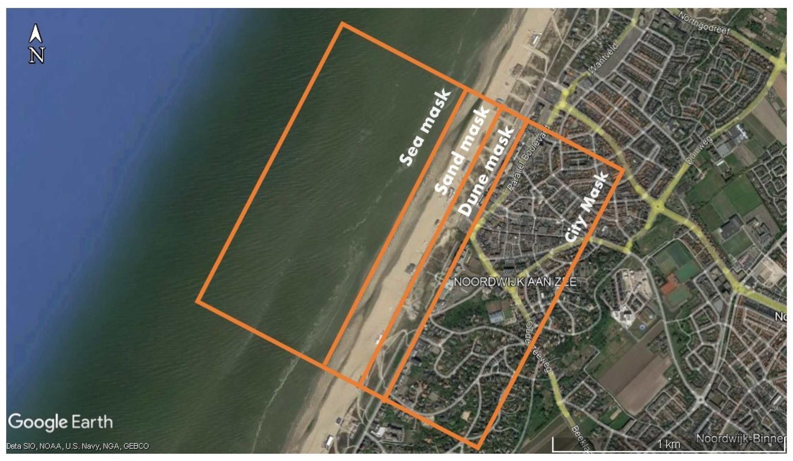
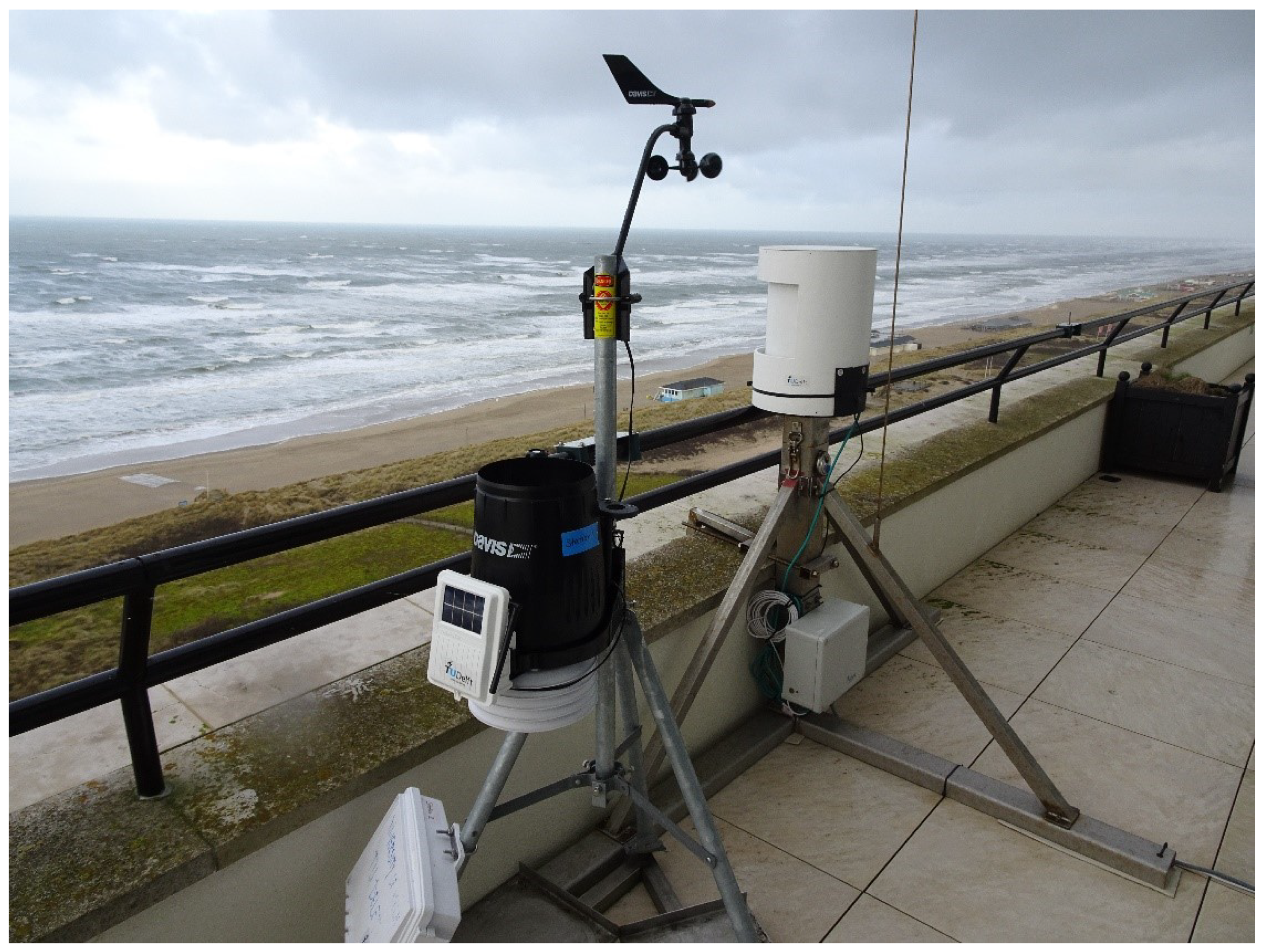
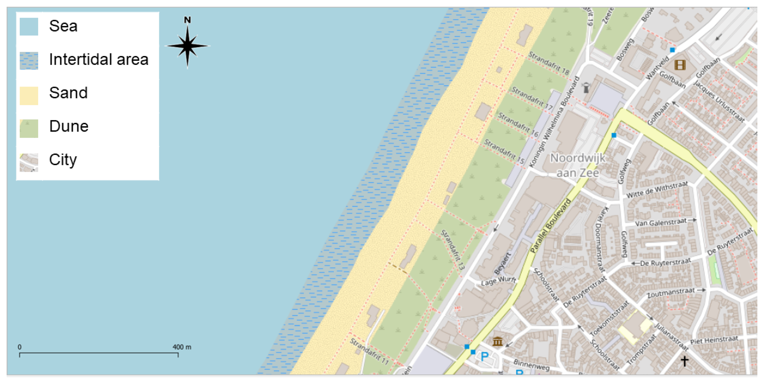
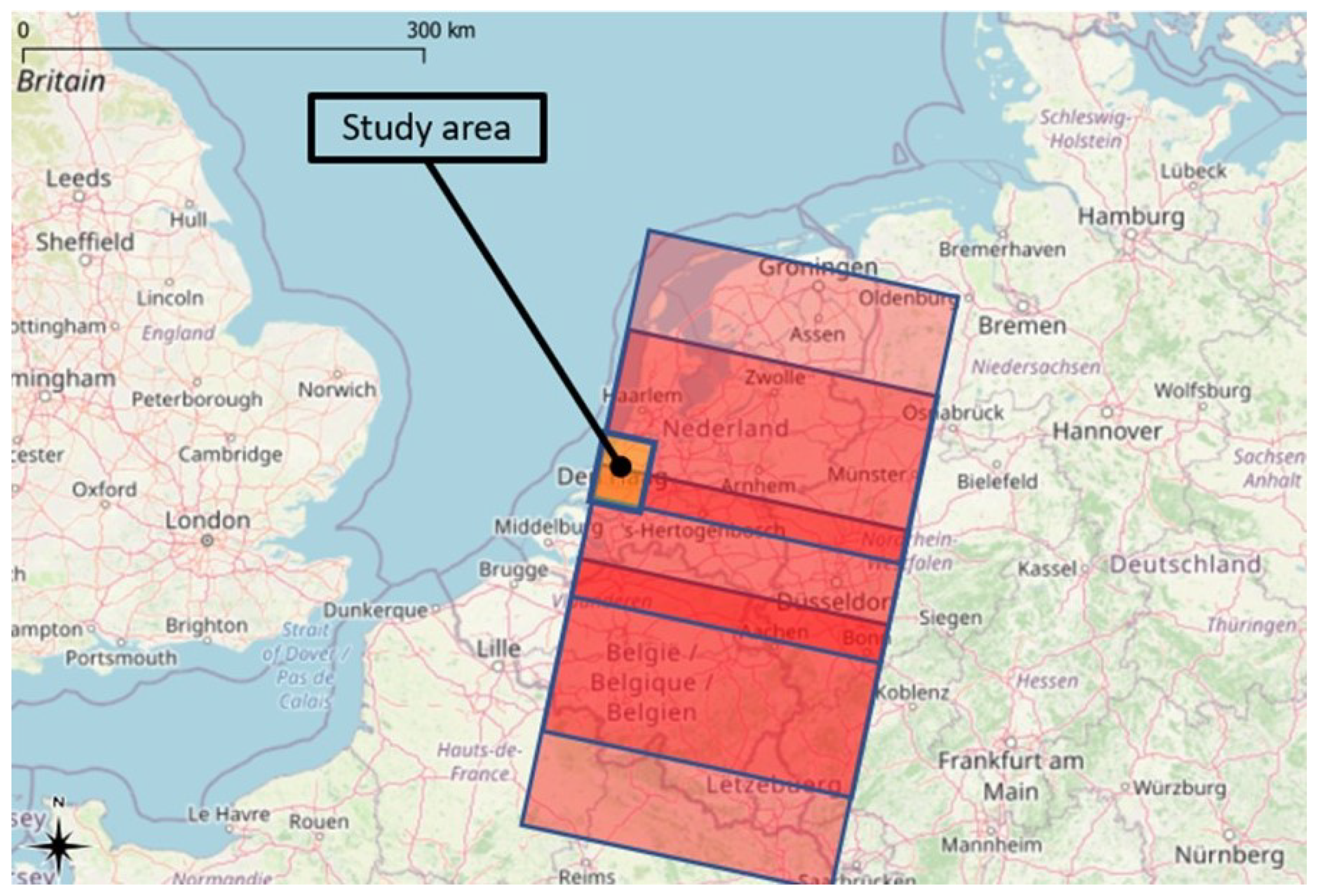
2.1. Study Area

The study site is a beach section at Noordwijk, located at 52.24°N, 4.42°E (Figure 1).

The area investigated covers a surface of about 100 km². Part of the area is covered by sea. A large part of the beach (∼130 m wide) consists of a dune area covered by vegetation. The dune area has not been taken into account for the analysis considering the presence of vegetation and the highly variable slopes which require a different approach for the investigation of the radar signal. The city area represents the section that is more heterogeneous. The considered beach area is relatively narrow ($\sim 140$ m wide in the case of low tide), consisting predominantly of fine quartz sand ($>90$%) [65]. We estimated the mean grain size to be ∼260 $\mathsf{\mu }$m using sieving methods from sediment collected within the top 2 mm. Fieldwork measurements were taken in order to estimate the shoreline position in case of high tide and low tide. These measurements have been used for the mask evaluations in Section 3.1.

2.2. Satellite Imagery and Pre-Processing

The considered Sentinel-1 dataset collected over the Dutch coast ranges from January 2018 until December 2019. The SAR data, in C band at $5.6$ cm wavelength, are available both in VV and VH polarization. A total of 106 and 108 images from a descending orbit (DSC37) have been used for VH and VV, respectively. The acquisition orbit selected was descending, parallel to the coastline, see Figure 2, to ensure optimal coverage of the area of interest. The dataset, provided in Interferometric Wide swath mode (IW), consists of Level-1 Single-Look Complex (SLC) products, where each image pixel is represented by a complex value and contains both amplitude and phase information. The imagery is geo-referenced using orbit and attitude data from the satellite. Each IW SLC image consists of a series of bursts.

IW SLC products are re-sampled to a common pixel spacing grid in range and azimuth. The pre-processing of the satellite imagery has been done by using the SNAP tool (https://step.esa.int/main/toolboxes/snap/, accessed on 1 October 2020). The data were split by selecting the subswath, the burst and the polarization, and then co-registered. After co-registration, a subset containing the area of interest was cropped. For each pixel, the amplitude has been automatically evaluated as a function of the given complex number. We decided not to apply any sort of noise correction or mitigation on the amplitude value in order to keep the original information. In order to have amplitude values easily comparable in the figures, given the amplitude $A=\sqrt{i^2+q^2}$, the amplitude values used in this paper are obtained as $lo{g}_{10}\left(A\right)$.

2.3. Ancillary Data

Numerous meteorological stations continuously monitor the area of interest providing detailed variables. For the present study, information regarding wind (speed and direction) and precipitation accumulation at the time of the satellite pass were collected. All the weather data used in this study have been collected at the moment of the satellite pass. Instantaneous wind values for both speed and direction have been used, whilst for the rain, the precipitation accumulation has been considered, which is the sum of precipitation over a certain period of time. In particular, the precipitation accumulation over the past 7 h before the satellite pass has been considered. Four weather stations were selected since they provide the type of data and the temporal sampling required: two amateur and two professional meteorological stations. The amateur meteorological stations are located in Noordwijk (52.25°N, 4.43°E) and Katwijk (52.19°N, 4.41°E), both on the beach and close to the area of interest (respectively 1 km and 7 km from the area of interest); the professional weather stations are located at IJmuiden (52.463°N, 4.555°E) and Schiphol (52.318°N, 4.790°E), i.e., 31 km and 34 km from the area of interest, respectively. The datasets of the two KNMI (KNMI: Koninklijk Nederlands Meteorologisch Instituut, https://www.knmi.nl/nederland-nu/klimatologie/daggegevens, accessed on 1 October 2020) weather stations have high correlation coefficients with each other concerning the wind and rain variables. The wind data set of station Noordwijk during the two years is not as complete as station Katwijk, while the opposite goes for the rain dataset, where the station in Katwijk does not contain a fully complete dataset. The two amateur weather stations at Katwijk and Noordwijk are closely correlated with the KMNI stations and therefore they have been used as a reliable source for wind (speed and direction) and precipitation accumulation. Tidal condition information is provided by the Dutch authorities (Rijkswaterstaat) and is freely accessible online (https://www.worldtides.info/copyright, accessed on 1 October 2020). As for the weather conditions, tidal conditions at the time of the satellite pass have been considered.

3. Methods

3.1. Mask Selection

In the subset cropped at the end of the SAR pre-processing, four masks have been classified depending on the coverage as shown in Figure 3. The analysis of the amplitude has been performed per mask.

The four masks include: (i) a city area, which has been mostly used for evaluating the low-variability pixels and for data calibration; (ii) a dune area, including the dunes and vegetation zone located between the city and the beach, which has not been evaluated due to the complexity of the area (including slope and vegetation) and to its limited relevance for the present study; (iii) the beach area, including the entire sandy area. It consists in a dry part of the beach, not affected by tidal cycles but only by weather condition and human activities; this area also includes small constructions such as bars, restaurants, temporary stands, or boats permanently or temporarily located on the beach; it also includes the intertidal area, which is the area affected by the tides and which can be either partially dry or covered by sea depending on the tidal condition; (iv) the shallow sea area, just behind the main surf where waves are breaking, particularly relevant for the analysis of the wind conditions.

3.2. Amplitude Calibration

The SAR signal is typically affected by soil properties with the same order of magnitude as the signal wavelength [66], i.e., the surface roughness, and the dielectric properties and water content. We performed a sensitivity analysis to understand how the amplitude of Sentinel-1 from a coastal area is affected by the above-mentioned parameters. As a first step, an empirical local calibration of the images has been done. The city mask showed the least amplitude variability over time. Within this mask, the 25% of the pixels with the least amplitude variability (smallest standard deviation) over time have been selected and used for calibrating the images. This calibration has been done separately for the VV and the VH polarization. For the VH polarization, the mean amplitude over time for the selected pixels ranges between 0.92 and 1.13, whilst for VV polarization it ranges between 0.75 and 1.11. Figure 4 (left), for VV polarization, shows that there is no significant correlation ($r=0.25$) between the amplitude values of the city mask and the ones of the sand mask (e.g., caused by noise in the image). Figure 4 (right) shows instead a high correlation ($r=0.84$) between the sand and sea masks. For VH polarization, the correlation factor between city and sand mask is $r=0.05$ and between the sea and sand it is $r=0.68$. As the morphology of the study area shows (Figure 1), the heterogeneity of the masks taken into consideration is different. At the SAR resolution, the coverage of sand and of the sea mask can be considered homogeneous whilst the city mask includes different anthropogenic structures (buildings, grass/agricultural fields, streets, etc.). In Figure 4 (left), when investigating the correlation between city and sand mask at a pixel resolution, there are pixels with different degrees of correlation depending on the pixel coverage in the city mask, but when considering the entire city mask, the correlation factor is low. In Figure 4 (right) instead, two homogeneous areas are compared (sand and sea) and their correlation is high. The color bar of Figure 4 expresses the wind intensity: it shows that there is no clear correlation between the wind speed and the city mask, whilst the wind speed shows a more explicit influence on the sand and sea areas.

After calibrating all the images relative to the low variability area, we analyze the mean amplitude value of the considered masks as a function of time for both the polarizations VV and VH, see Figure 5 and Figure 6. For VV polarization, the highest values occur for the city mask, which is also shows the least variability (13% over time) and the least influenced by the weather conditions.

The maximum variability (31%) and the lowest mean values occur in the shallow sea area. We hypothesize that is that this is mainly due to the wind, which affects the surface roughness. A high variability (20%) also occurs in the sandy area. This can be due to anthropogenic factors (e.g., the presence of boats or temporary stands during summer, people, tractors, sand deposits built during winter around the buildings, the effect on the moisture and on the roughness of the tide), weather conditions (the wind reshaping the sand), and tidal conditions. For VH polarization, similar conditions occur but the variability of the three masks is lower: City, 6%; Sand, 15%; Sea, 11%. Thus, it appears that VV polarization is more sensitive to phenomena affecting both the sand and the sea mask. Figure 5 and Figure 6 also represent VV and VH ranges in the city, the sandy and the shallow sea mask. They show how this maximum value decreases going from the city towards the sea. Both polarizations show the same behavior, but the values in VH polarization always range lower than VV.

This analysis also showed that it is not possible to identify a temporal or a seasonal trend in the amplitude values.

3.3. Roughness Analysis

The purpose of this section is to evaluate the roughness of the beach surface by using a Terrestrial Laser Scanner (TLS), and evaluating the Root Mean Square Heights (RMSH) for each SAR pixel. These values will be compared to the SAR amplitude. The TLS used for this analysis is a Riegl-VZ2000, which was installed in July 2019 on the upper balcony of a building at 156 m distance from the beach area of Noordwijk (see Figure 7).

It has collected data for two years. The field of view is $\sim 1$ km by $\sim 300$ m and contains a part of the dunes, the beach and the intertidal zone during high and low tide. This yields detailed information on the beach morphology.

3.3.1. Terrestrial Laser Scanner

Every hour a dataset containing a 3D representation of the scanned area and the backscatter intensity is collected by the TLS. The Riegl VZ-2000 operates with an accuracy of 8 mm and a precision of 5 mm [67] in the near-infrared. The laser beam divergence is $0.3$ mrad, and its field of view is 100° horizontal and 360° vertical. Each point is associated with a horizontal angle $\varphi$ and vertical angle $\theta$. These coordinates are automatically converted into ($x,y,z$) coordinates relative to the TLS. The laser scans the area every hour in low resolution, which corresponds to $0.03$° angular point spacing (about 30 cm point spacing at the waterline). Each data point contains ($x,y,z$) coordinates and reflectance. Low-resolution data points, in terms of ($x,y,z$) coordinates, converted to the geographic coordinate system, have been used to perform the relation with SAR data.

3.3.2. RMSH Evaluation

In order to evaluate the RMSH index over the study area, the following procedure has been adopted:

1.

Creation of two different stacks of images. The first stack contains the coregistered Sentinel-1 images, from the same orbit used for the study described above, acquired during the period of TLS activity, from July 2019 until April 2020. The second stack contains the coregistered TLS images acquired at the same local time of Sentinel-1 pass over the study area. The two stacks contain 30 images which have been therefore acquired on the same day and at the same local time.

2.

TLS and SAR images have been coregistered: each TLS data point has been associated to the closest SAR pixel center. After the match, at least a hundred TLS data points are associated with each SAR pixel. SAR pixels with a low number of TLS data points have not been considered.

3.

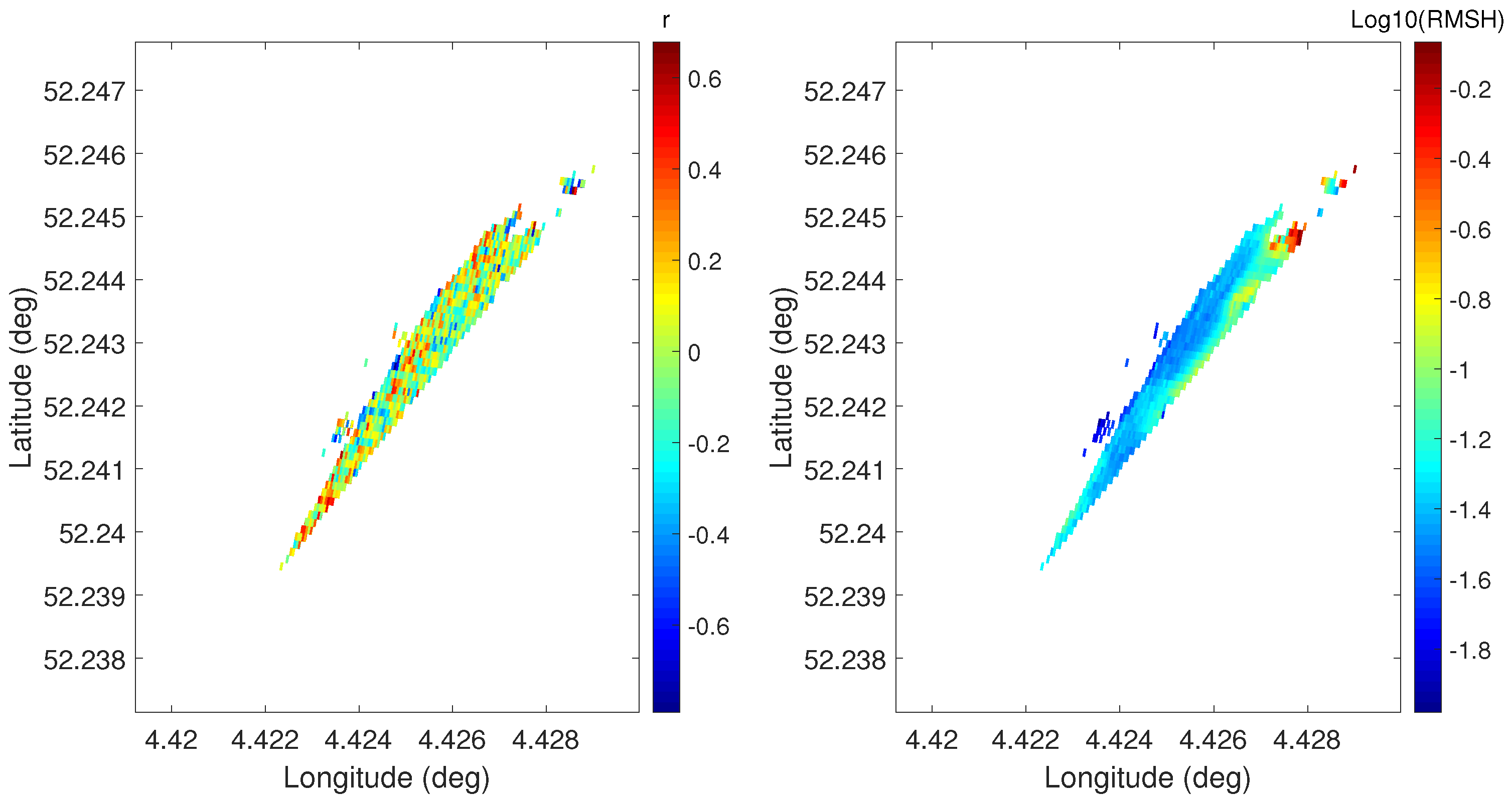
The z values of the data points belonging to each SAR pixel have been interpolated on a $M\times N$ pixels grid (with a resolution of 0.1 × 10⁻⁵ degrees in latitude and longitude). For each grid, RMSH has been evaluated as in [52]:

$$\mathrm{RMSH}=\sqrt{\frac{1}{MN}\sum _{c=0}^{M-1}\sum _{r=0}^{N-1}{[z(x_c,y_r)-\mu ]}^2}$$

(1)

where:

M = number of columns;

N = number of rows;

c = column index;

r = row index;

$z(x_c,y_r)$ = z-value at position $x_c$,$y_r$;

$\mu$ = average z-value

4.

Using (1) each SAR pixel is characterized by its own local RMSH value, with a $\sim 10$ cm resolution.

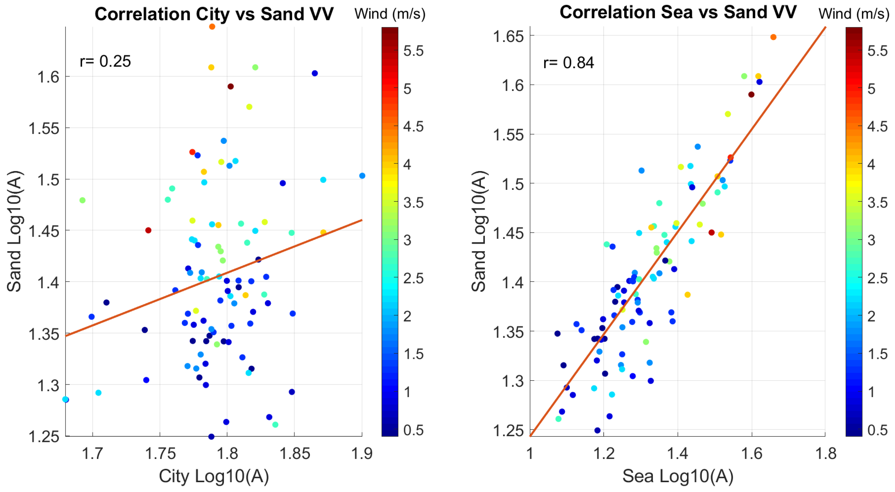
3.3.3. RMSH Correlation

In total, $\sim 400$ pixels have been considered in the present analysis. For each SAR pixel, a time-series has been developed containing RMSH values as a function of ${log}_{10}\left(A\right)$, and their correlation has been evaluated. The correlation maps between RMSH values and ${log}_{10}\left(A\right)$ (Figure 8 (left)) have been compared to the mean RMSH for each pixel (Figure 8 (right)). Figure 8 (right) shows how, excluding the upper right area corresponding to the end of the dunes area, RMSH values are almost constant over the beach, and that they get lower moving toward the sea. Figure 8 (left) shows how the range of the correlation values is very wide (from $-0.65$ up to $+0.65$). No evident correlation seems to exist between RMSH values and correlation values, and that the relation between RMSH and ${log}_{10}\left(A\right)$ could have a stochastic nature.

4. Results

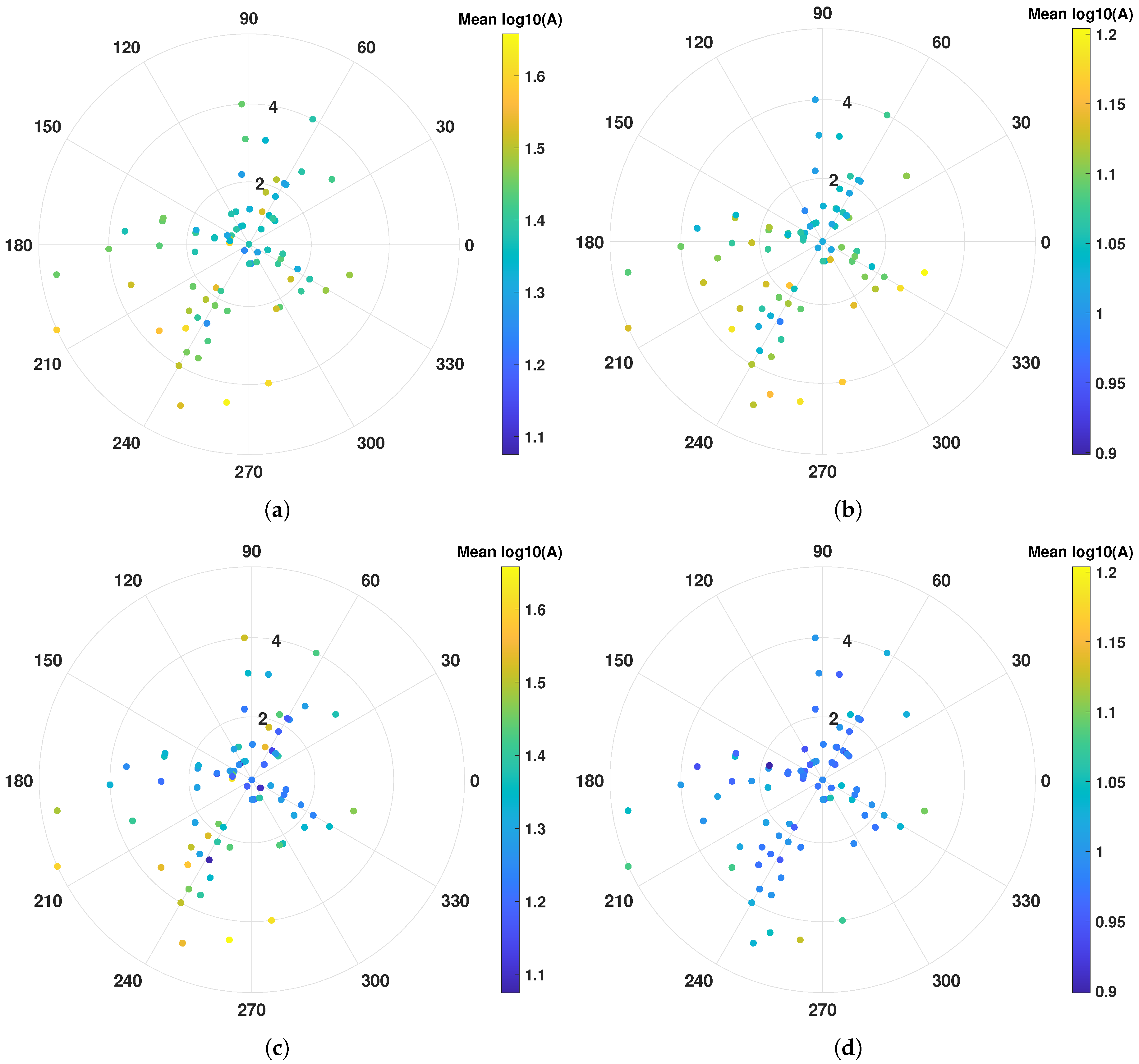
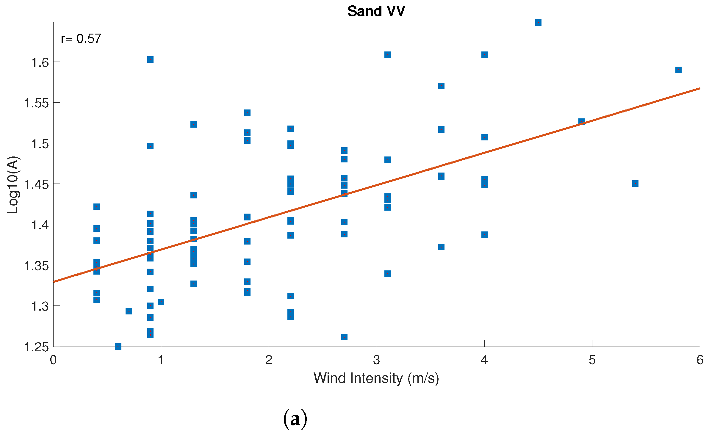
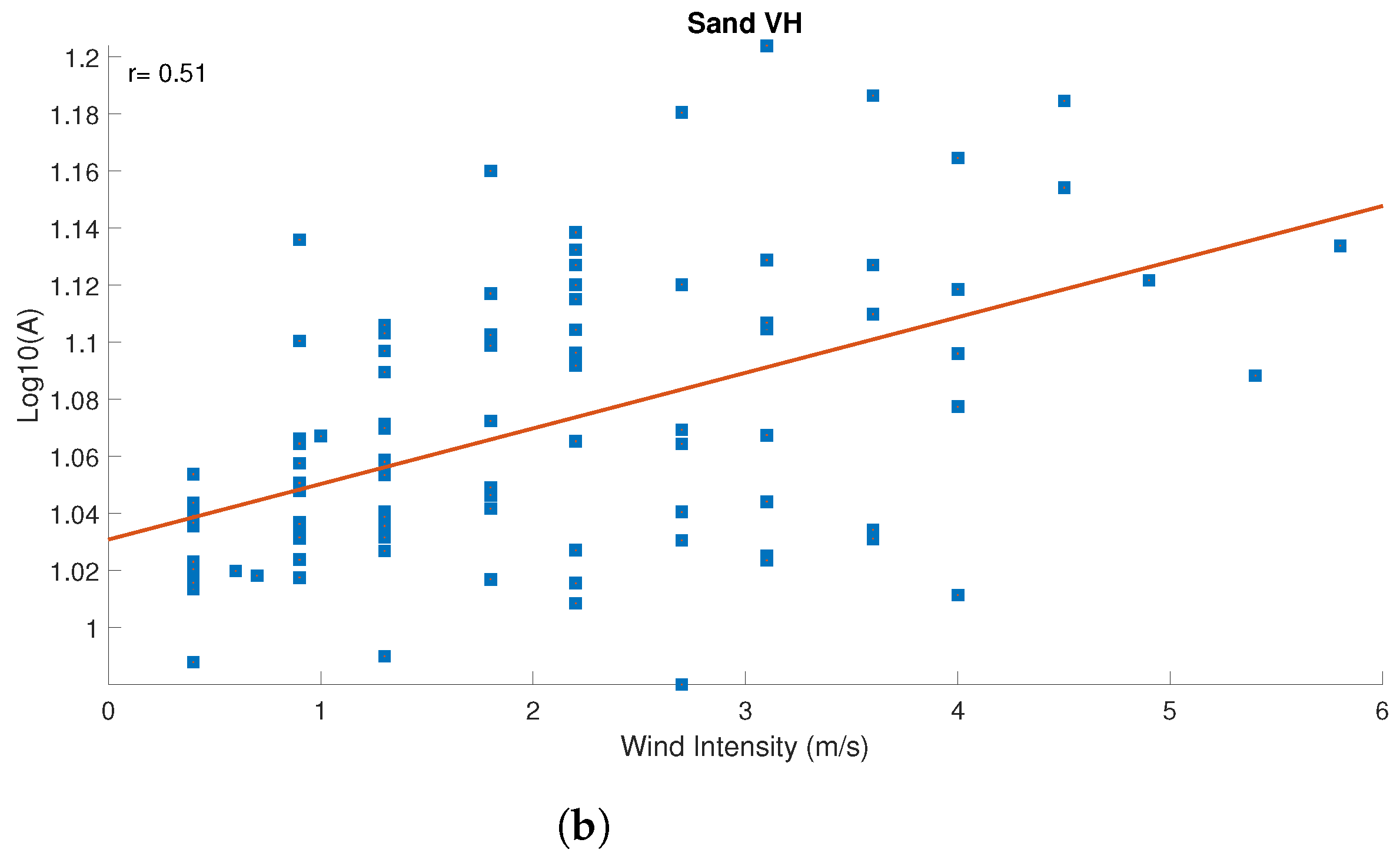
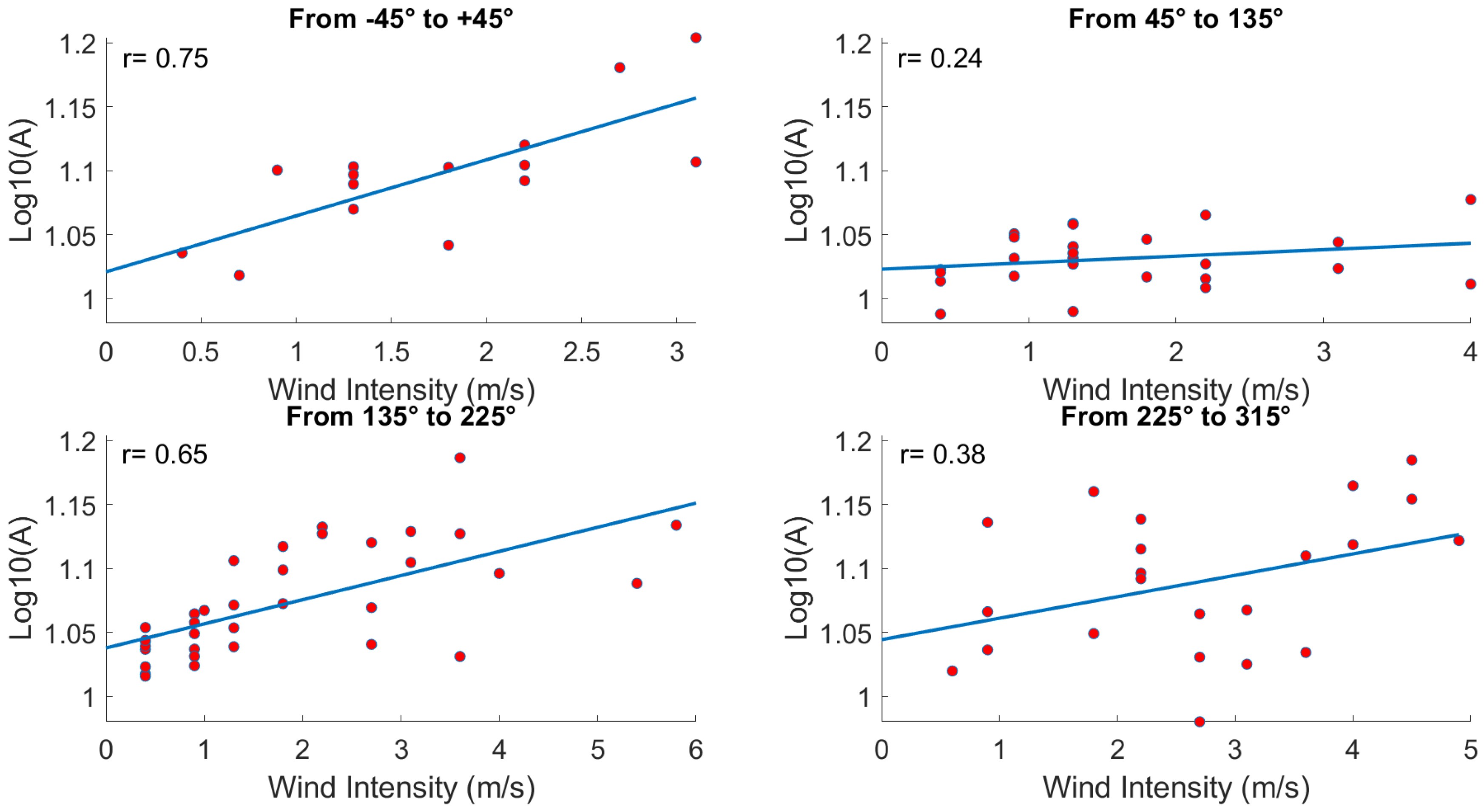
4.1. Wind Analysis

To investigate the sensitivity of the amplitude signal to the wind, scatter plots of the amplitude at VV and VH polarization versus wind intensity and speed were generated. Figure 9 shows respectively the plots of the wind speed and direction as a function of the amplitude mean value for the sand and sea masks in both VV and VH polarizations. The amplitude mean value is shown in the color bar, on a logarithmic scale. A dependence of amplitude on the wind direction can be noticed both in the two masks and in the two polarization.

Considering the sand mask, the distribution of wind intensity is associated with low or high amplitude depending on the wind direction. For some wind angles (i.e., 210°–240°), the dependence of the amplitude on the wind is more considerable. The same considerations can be done for the sea mask, where it can be noticed how low amplitude values are associated with low wind intensity, which increases going towards higher amplitude values. A dependence on the wind direction can be also noticed, e.g., in the range 270°–360°. In general, for both polarizations and both masks, a high wind intensity is associated with high amplitude values.

The correlation factor between the amplitude and the wind intensity has been evaluated for both polarizations and for all the masks. The highest correlation occurs obviously in the sea mask for both polarizations, with a correlation factor $r=0.56$ for VH and $r=0.62$ for VV. Polarizations VV and VH also show a significant correlation on the sand area, where the correlation factors are $r=0.57$ and $r=0.51$ respectively, see Figure 10a,b.

It is interesting to note that the correlation increases or decreases depending on the wind direction. Figure 11 shows how the correlation factor in the sandy area has the highest value of 0.75 for wind direction $-45$°–$45$° and a minimum value of 0.24 for wind direction 45°–135°.

Further analysis of the amplitude of the city area shows a very low correlation both with the wind direction and with the wind speed (correlation factor between amplitude and wind speed: $r=0.2$ for VH and $r=0.1$ for VV).

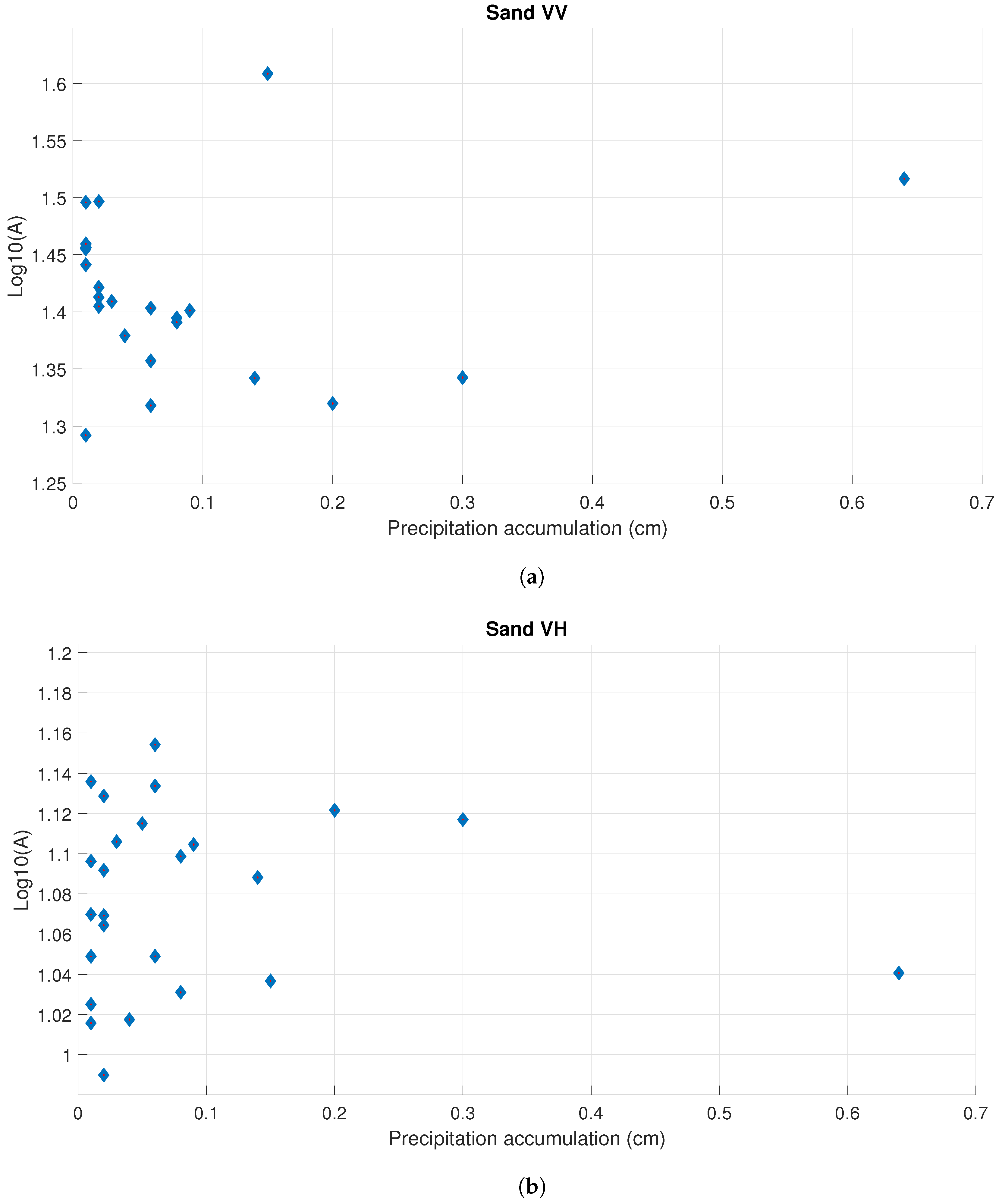
4.2. Rain Condition

The rain conditions were also taken into consideration. Over the two-year dataset, 25 days with a precipitation accumulation $>0$ at the time of the satellite pass were registered. These days were used to generate a scatter plot of the amplitude value (VV and VH polarizations) versus the precipitation accumulations. Despite the low number of days with positive precipitation accumulation at the moment of the satellite pass during the two years analyzed, these data were used to generate a scatter plot of the amplitude value (VV and VH polarizations) versus the precipitation accumulations in order to evaluate any possible relation. No particular correlation or trend can be noticed in this analysis for all the considered masks (see Figure 12), and the effect of the rain on the SAR signal is not relevant to get further information on sandy areas.

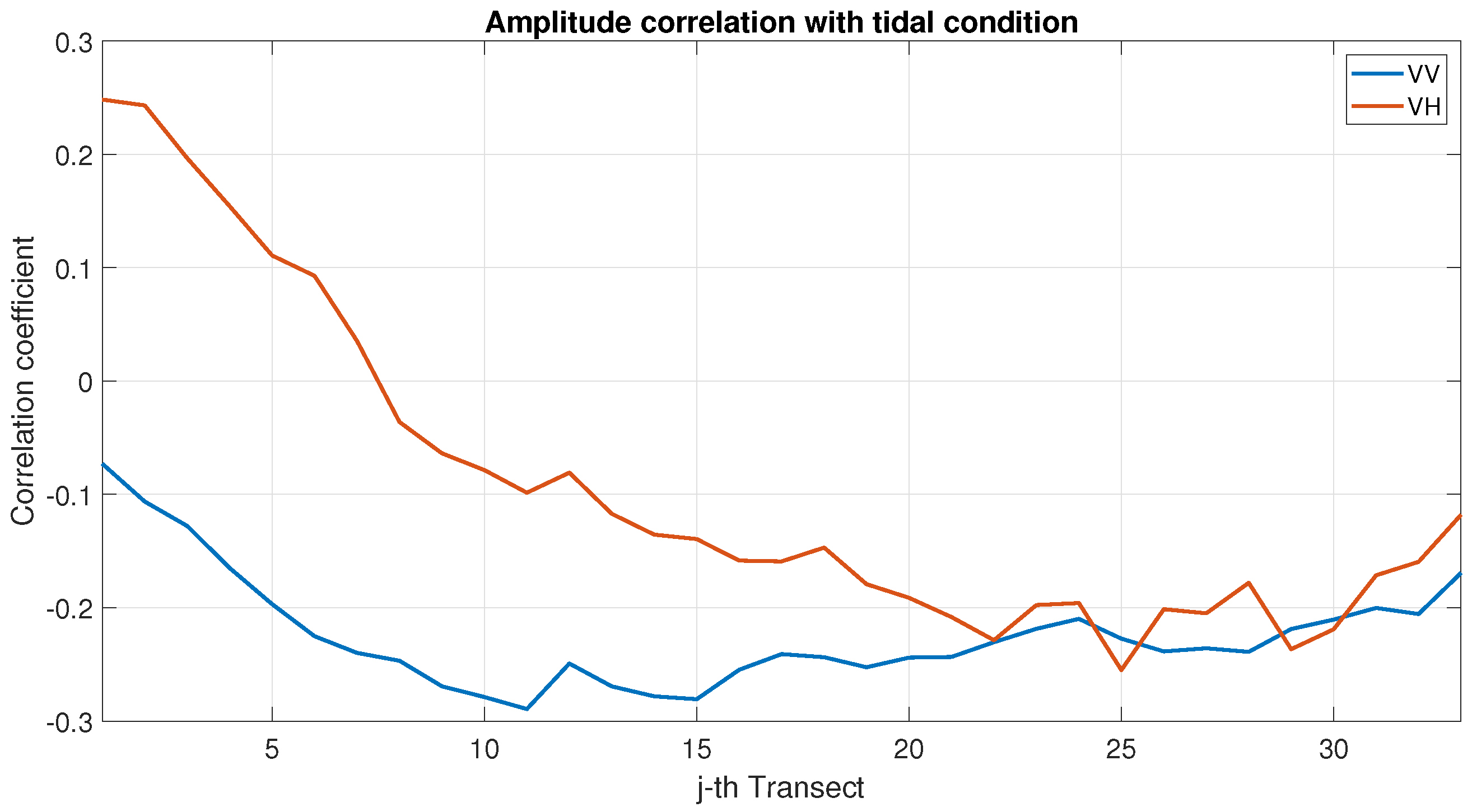
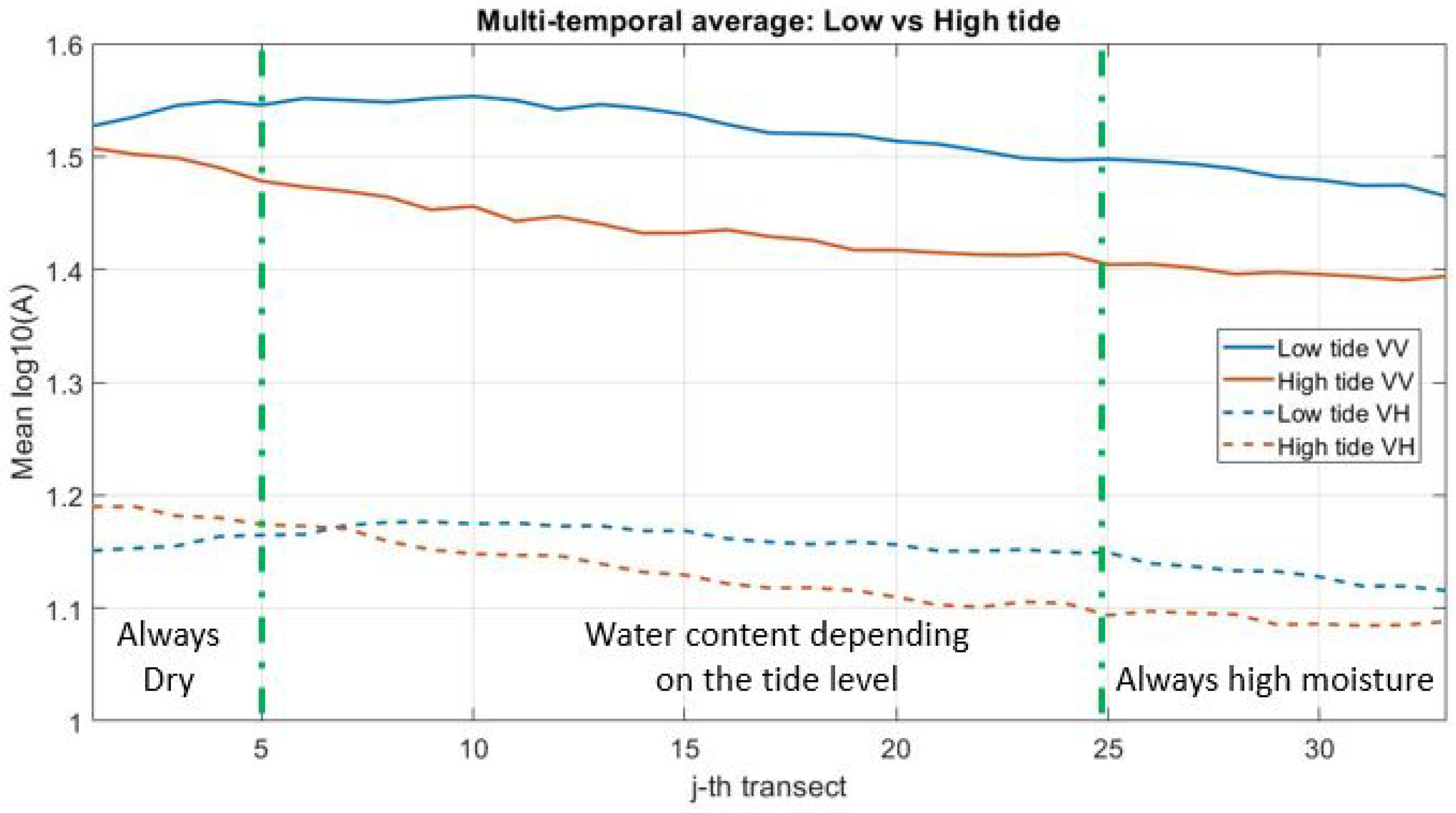
4.3. Tidal Condition Analysis

The sensitivity analysis of the amplitude signal to the tidal condition, which is connected to the sensitivity of the SAR signal to the soil moisture and to the presence of water in the pixels, has been carried out in the following way. The considered area covers a surface of $0.14$ km², and it corresponds to the intertidal mask plus the last part of the dry mask. Sea waves can reach this area in case of very high wind with a specific direction. It is reasonable to think that the anthropic influence on this area is particularly low. This area has been divided into 33 transects, $3.5$ m wide, parallel to the waterline. For each transect, the mean multi-temporal amplitude both for VV and VH polarizations have been evaluated (Figure 13). It can be noticed the decreasing trend going from the dry transect ($j=1$) towards the sea ($j=33$). Both polarizations show about 6% decrease of the $log\left(A\right)$ along the transects. The last transects have always either seawater (high tide) or high moisture content (low tide), whilst the water content of the intermediate transects depends on the tide level. When evaluating the correlation of the amplitude for each transect with the tidal condition (Figure 14), it is noticed that there is a sign change. For VH polarization, the correlation with the tide ranges from $+0.25$ to $-0.25$ going from the dry transect towards the sea. The correlation factor gets negative with the increase of the water content along the transects (therefore the amplitude decreases). VV polarization seems to have a different sensitivity and the correlation factor is negative for all the analyzed transects. The last plot shows the amplitude variation when separating the low and the high tidal condition (Figure 15). For VH polarization, in the case of high tide (higher water level in the transects), the amplitude values are in general lower than the case of low tide (less water content). This does not occur for the transects which are always dry. VV polarization shows the same trend but a different sensitivity and higher amplitude values. This analysis can be further investigated in order to understand to what extent it is possible to detect the water content on the sand considering the sensitivity of the two polarizations.

5. Discussion

5.1. Weather Correlation

In Section 4.1 and Section 4.2 we presented the results obtained by correlating SAR amplitude and weather information collected at the moment of the satellite pass. Further analysis on different typologies of weather dataset have been conducted in order to select the appropriate data for the purpose of the present study.

Regarding the wind data, tests have been conducted by using a daily mean speed value instead of an instantaneous value. The results obtained by comparing the SAR amplitude with the daily mean wind values led to slightly lower correlation values. This lower correlation has been attributed to the days when a sudden change in wind speed (in particular a sudden increase in speed) occurred in the hours before the satellite pass. During the days with stable wind conditions, no difference could be retrieved in the correlation with the SAR amplitude; therefore, it has been decided to use instantaneous values. Regarding the precipitation dataset, it has been decided to consider the precipitation accumulation instead of the instantaneous value in order to take into consideration the possible effect of the sand moisture which could affect the SAR signal; the use of an instantaneous precipitation value would have excluded the consideration of this factor in all the cases in which the sand is wet due to previous precipitation phenomena, but there is no rain at the moment of the satellite pass. However, as shown in Section 4.2, the low amount of days with positive precipitation accumulation values at the moment of the satellite pass did not show any particular correlation with the SAR amplitude.

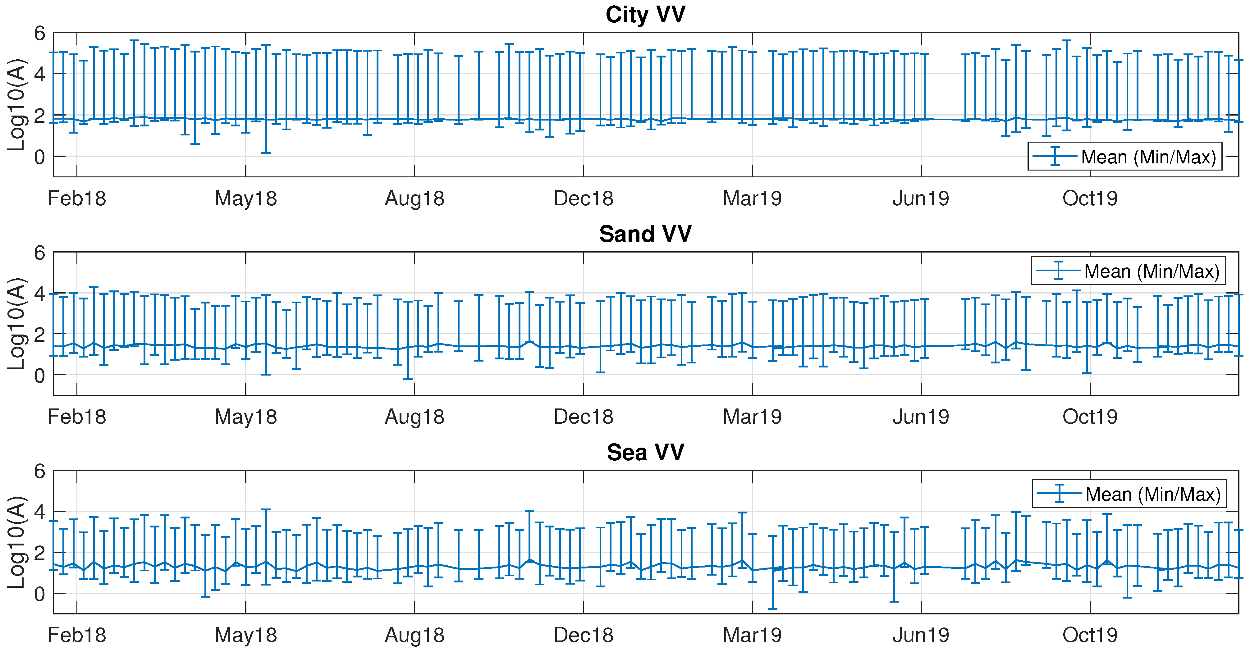
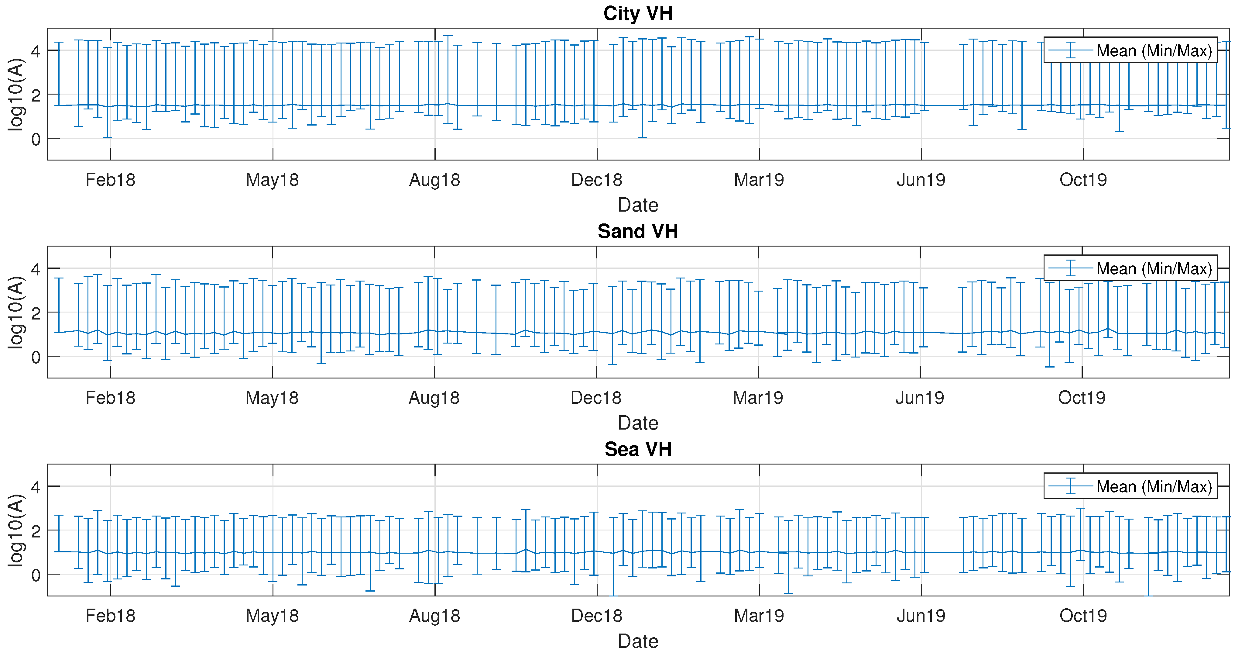
5.2. Amplitude Time Series

As presented in Section 2.2, a SAR time series has been created from January 2018 to December 2019. Further analyses have been conducted in order to understand whether a SAR amplitude trend (e.g., monthly, seasonal, or annual) exists in the considered masks. Results of this analysis did not show any particular SAR trend which could be attributed to seasonal or annual variations, therefore the entire stack of SAR data has been used to create a time series. Monthly, seasonal, and annual trends of the amplitude related to the tide have also been investigated, and also in this case results showed that no trend is particularly evident.

5.3. Roughness Influence

As shown in Figure 4, sea and sand masks are highly correlated. Both in sea and sand masks, the distribution of wind intensity is associated with low or high amplitude depending on the wind direction, and the correlation factor between amplitude and wind intensity significantly increases or decreases when focusing the analysis on specific wind direction. The same situation occurs in the sea mask. On the other hand, mean RMSH analysis showed that no evident correlation seems to exist between RMSH and amplitude. Considering these phenomena, the hypothesis is that the SAR signal—for the considered wavelength (C band) and the considered orbit direction and angle of view on the study area—on sandy areas, might be related to the directional variation of the roughness of the surface more than on variation of the height of the surface points represented by the RMSH. Therefore specific wind directions which cause directional surface roughness variation on the sand give a higher correlation with the backscatter signal, compared to other wind directions. In the present study, the mean evaluated RMSH is on the order of a decimeter, roughly twice the dimension of the SAR wavelength. Different orders of magnitude of the RMSH, as well as different SAR bands or orbit directions, might also affect the results.

6. Conclusions

This paper presents the results of a feasibility study intended to gain insight into the potential and limitations of SAR imagery for the retrieval of soil properties over coastal areas. The most relevant result is a strong correlation between the amplitude evaluated on the sandy area, both for VV and VH polarizations, and the local wind. The distribution of wind intensity is associated with low or high amplitude depending on the wind direction. The rain conditions were taken into consideration by exploiting the precipitation accumulation on the beach of Noordwijk at the moment of the satellite pass and no particular correlation or trend of the amplitude could be noticed. Future studies could take into consideration the use of different weather datasets for both wind and rain (e.g., longer precipitation accumulation time or longer time series for the precipitation phenomena; different mean for the wind speed value, or the influence of wind direction over the hours before the satellite pass) to demonstrate whether a higher or lower correlation with SAR signal exists. The sensitivity analysis of the amplitude signal to the tidal condition has been carried out considering transects of the beach parallel to the coastline in the intertidal area. Both polarizations show a decreasing trend of the amplitude along the transects, moving from the dry area of the beach towards the sea. The correlation coefficient between the amplitude and the tide level gets negative with the increase of the water content along the transects.

In the present work, only environmental phenomena have been taken into consideration. In future works, the effect of anthropogenic activities could be added to have a more complete overview of the SAR backscatter variations on coastal areas. Future work will also include a deeper exploitation of SAR data as an input for providing a better knowledge of the causal empirical relationship between weather phenomena and protective capability of beaches, i.e., thanks to the creation of classification maps of the coastal environment (in particular shoreline position and separation between intertidal and dry beach area) which, with a long-term analysis, will allow the understanding of their multitemporal evolution depending on natural phenomena. A deeper investigation on the different contributions of moisture and roughness (i.e., by using SAR images with higher resolution, dedicated SLC processing or different SAR bands and orbit directions) on the amplitude signal is necessary to understand whether the SAR signal can be exploited to retrieve more detailed information both on sand moisture and on the effect of the wind on the surface roughness. In particular, deeper investigation on the surface roughness can show in which way this phenomena affects the SAR signal. This information can be of great importance in the field of aeolian transport, considering the unique SAR capability of worldwide coverage with continuous monitoring of the coastal areas.

References

- Burkett, V.; Davidson, M. Coastal Impacts, Adaptation, and Vulnerabilities; Springer: Washington, DC, USA, 2012. [Google Scholar]
- Wright, D.J. Ocean Solutions, Earth Solutions; Esri Press: Redlands, CA, USA, 2015. [Google Scholar]
- Klemas, V.V. The role of remote sensing in predicting and determining coastal storm impacts. J. Coast. Res. 2009, 25, 1264–1275. [Google Scholar] [CrossRef] [Green Version]
- Bochev-Van der Burgh, L.; Wijnberg, K.M.; Hulscher, S.J. Decadal-scale morphologic variability of managed coastal dunes. Coast. Eng. 2011, 58, 927–936. [Google Scholar] [CrossRef]
- Keijsers, J.G.; Giardino, A.; Poortinga, A.; Mulder, J.P.; Riksen, M.J.; Santinelli, G. Adaptation strategies to maintain dunes as flexible coastal flood defense in The Netherlands. Mitig. Adapt. Strateg. Glob. Chang. 2015, 20, 913–928. [Google Scholar] [CrossRef] [Green Version]
- Benveniste, J.; Cazenave, A.; Vignudelli, S.; Fenoglio-Marc, L.; Shah, R.; Almar, R.; Andersen, O.B.; Birol, F.; Bonnefond, P.; Bouffard, J.; et al. Requirements for a coastal hazards observing system. Front. Mar. Sci. 2019, 6, 348. [Google Scholar] [CrossRef] [Green Version]
- Mason, D.; Gurney, C.; Kennett, M. Beach topography mapping—A comparsion of techniques. J. Coast. Conserv. 2000, 6, 113–124. [Google Scholar] [CrossRef]
- Mielck, F.; Hass, H.C.; Betzler, C. High-resolution hydroacoustic seafloor classification of sandy environments in the German Wadden Sea. J. Coast. Res. 2014, 30, 1107–1117. [Google Scholar] [CrossRef]
- Porskamp, P.; Rattray, A.; Young, M.; Ierodiaconou, D. Multiscale and hierarchical classification for benthic habitat mapping. Geosciences 2018, 8, 119. [Google Scholar] [CrossRef] [Green Version]
- Choi, C.; Kim, D.J. Optimum baseline of a single-pass In-SAR system to generate the best DEM in tidal flats. IEEE J. Sel. Top. Appl. Earth Obs. Remote Sens. 2018, 11, 919–929. [Google Scholar] [CrossRef]
- Salameh, E.; Frappart, F.; Almar, R.; Baptista, P.; Heygster, G.; Lubac, B.; Raucoules, D.; Almeida, L.P.; Bergsma, E.W.; Capo, S.; et al. Monitoring beach topography and nearshore bathymetry using spaceborne remote sensing: A review. Remote Sens. 2019, 11, 2212. [Google Scholar] [CrossRef] [Green Version]
- Atherton, R.J.; Baird, A.J.; Wiggs, G.F. Inter-tidal dynamics of surface moisture content on a meso-tidal beach. J. Coast. Res. 2001, 17, 482–489. [Google Scholar]
- Namikas, S.; Edwards, B.; Bitton, M.; Booth, J.; Zhu, Y. Temporal and spatial variabilities in the surface moisture content of a fine-grained beach. Geomorphology 2010, 114, 303–310. [Google Scholar] [CrossRef]
- Davidson-Arnott, R.G.; MacQuarrie, K.; Aagaard, T. The effect of wind gusts, moisture content and fetch length on sand transport on a beach. Geomorphology 2005, 68, 115–129. [Google Scholar] [CrossRef]
- Bauer, B.; Davidson-Arnott, R.; Hesp, P.; Namikas, S.; Ollerhead, J.; Walker, I. Aeolian sediment transport on a beach: Surface moisture, wind fetch, and mean transport. Geomorphology 2009, 105, 106–116. [Google Scholar] [CrossRef]
- Ellis, J.T.; Sherman, D.J.; Farrell, E.J.; Li, B. Temporal and spatial variability of aeolian sand transport: Implications for field measurements. Aeolian Res. 2012, 3, 379–387. [Google Scholar] [CrossRef]
- De Vries, S.; de Vries, J.V.T.; Van Rijn, L.; Arens, S.; Ranasinghe, R. Aeolian sediment transport in supply limited situations. Aeolian Res. 2014, 12, 75–85. [Google Scholar] [CrossRef]
- McKenna-Neuman, C.; Nickling, W. A theoretical and wind tunnel investigation of the effect of capillary water on the entrainment of sediment by wind. Can. J. Soil Sci. 1989, 69, 79–96. [Google Scholar] [CrossRef]
- Cornelis, W.; Gabriels, D. The effect of surface moisture on the entrainment of dune sand by wind: An evaluation of selected models. Sedimentology 2003, 50, 771–790. [Google Scholar] [CrossRef]
- Ahmed, A.; Zhang, Y.; Nichols, S. Review and evaluation of remote sensing methods for soil-moisture estimation. SPIE Rev. 2011, 2, 028001. [Google Scholar]
- Wiggs, G.; Baird, A.; Atherton, R. The dynamic effects of moisture on the entrainment and transport of sand by wind. Geomorphology 2004, 59, 13–30. [Google Scholar] [CrossRef]
- Yang, Y.; Davidson-Arnott, R.G. Rapid measurement of surface moisture content on a beach. J. Coast. Res. 2005, 21, 447–452. [Google Scholar] [CrossRef]
- Nield, J.M.; King, J.; Jacobs, B. Detecting surface moisture in aeolian environments using terrestrial laser scanning. Aeolian Res. 2014, 12, 9–17. [Google Scholar] [CrossRef]
- Nolet, C.; Poortinga, A.; Roosjen, P.; Bartholomeus, H.; Ruessink, G. Measuring and modeling the effect of surface moisture on the spectral reflectance of coastal beach sand. PLoS ONE 2014, 9, e112151. [Google Scholar]
- Di Biase, V.; Hanssen, R.F.; Vos, S.E. Sensitivity of near-infrared permanent laser scanning intensity for retrieving soil moisture on a coastal beach: Calibration procedure using in situ data. Remote Sens. 2021, 13, 1645. [Google Scholar] [CrossRef]
- McKenna Neuman, C.; Langston, G. Measurement of water content as a control of particle entrainment by wind. Earth Surf. Process. Landforms J. Br. Geomorphol. Res. Group 2006, 31, 303–317. [Google Scholar] [CrossRef]
- Darke, I.; Neuman, C.M. Field study of beach water content as a guide to wind erosion potential. J. Coast. Res. 2008, 24, 1200–1208. [Google Scholar] [CrossRef]
- Delgado-Fernandez, I.; Davidson-Arnott, R.; Ollerhead, J. Application of a remote sensing technique to the study of coastal dunes. J. Coast. Res. 2009, 25, 1160–1167. [Google Scholar] [CrossRef]
- Şekertekin, A.; Marangoz, A.M.; Abdikan, S. Soil moisture mapping using Sentinel-1A synthetic aperture radar data. Int. J. Environ. Geoinform. 2018, 5, 178–188. [Google Scholar] [CrossRef]
- Baghdadi, N.; Gaultier, S.; King, C. Retrieving surface roughness and soil moisture from synthetic aperture radar (SAR) data using neural networks. Can. J. Remote Sens. 2002, 28, 701–711. [Google Scholar] [CrossRef]
- Srivastava, H.S.; Patel, P.; Sharma, Y.; Navalgund, R.R. Large-area soil moisture estimation using multi-incidence-angle RADARSAT-1 SAR data. IEEE Trans. Geosci. Remote Sens. 2009, 47, 2528–2535. [Google Scholar] [CrossRef]
- Zribi, M.; Gorrab, A.; Baghdadi, N. A new soil roughness parameter for the modelling of radar backscattering over bare soil. Remote Sens. Environ. 2014, 152, 62–73. [Google Scholar] [CrossRef] [Green Version]
- Gorrab, A.; Zribi, M.; Baghdadi, N.; Mougenot, B.; Chabaane, Z.L. Potential of X-band TerraSAR-X and COSMO-SkyMed SAR data for the assessment of physical soil parameters. Remote Sens. 2015, 7, 747–766. [Google Scholar] [CrossRef] [Green Version]
- Fung, A.; Liu, W.; Chen, K.; Tsay, M. An improved IEM model for bistatic scattering from rough surfaces. J. Electromagn. Waves Appl. 2002, 16, 689–702. [Google Scholar] [CrossRef]
- Attarzadeh, R.; Amini, J.; Notarnicola, C.; Greifeneder, F. Synergetic use of Sentinel-1 and Sentinel-2 data for soil moisture mapping at plot scale. Remote Sens. 2018, 10, 1285. [Google Scholar] [CrossRef] [Green Version]
- Aubert, M.; Baghdadi, N.; Zribi, M.; Douaoui, A.; Loumagne, C.; Baup, F.; El Hajj, M.; Garrigues, S. Analysis of TerraSAR-X data sensitivity to bare soil moisture, roughness, composition and soil crust. Remote Sens. Environ. 2011, 115, 1801–1810. [Google Scholar] [CrossRef] [Green Version]
- Baghdadi, N.; Camus, P.; Beaugendre, N.; Issa, O.M.; Zribi, M.; Desprats, J.F.; Rajot, J.L.; Abdallah, C.; Sannier, C. Estimating surface soil moisture from TerraSAR-X data over two small catchments in the Sahelian Part of Western Niger. Remote Sens. 2011, 3, 1266–1283. [Google Scholar] [CrossRef] [Green Version]
- Zribi, M.; Kotti, F.; Lili-Chabaane, Z.; Baghdadi, N.; Issa, N.B.; Amri, R.; Amri, B.; Chehbouni, A. Soil texture estimation over a semiarid area using TerraSAR-X radar data. IEEE Geosci. Remote Sens. Lett. 2011, 9, 353–357. [Google Scholar] [CrossRef] [Green Version]
- Zribi, M.; Dechambre, M. A new empirical model to retrieve soil moisture and roughness from C-band radar data. Remote Sens. Environ. 2003, 84, 42–52. [Google Scholar] [CrossRef]
- Balenzano, A.; Mattia, F.; Satalino, G.; Davidson, M.W. Dense temporal series of C-and L-band SAR data for soil moisture retrieval over agricultural crops. IEEE J. Sel. Top. Appl. Earth Obs. Remote Sens. 2010, 4, 439–450. [Google Scholar] [CrossRef]
- Lievens, H.; Verhoest, N.E. Spatial and temporal soil moisture estimation from RADARSAT-2 imagery over Flevoland, The Netherlands. J. Hydrol. 2012, 456, 44–56. [Google Scholar] [CrossRef]
- Jacome, A.; Bernier, M.; Chokmani, K.; Gauthier, Y.; Poulin, J.; De Sève, D. Monitoring volumetric surface soil moisture content at the La Grande basin boreal wetland by radar multi polarization data. Remote Sens. 2013, 5, 4919–4941. [Google Scholar] [CrossRef] [Green Version]
- Paloscia, S.; Pettinato, S.; Santi, E. Combining L and X band SAR data for estimating biomass and soil moisture of agricultural fields. Eur. J. Remote Sens. 2012, 45, 99–109. [Google Scholar] [CrossRef]
- Kim, S.B.; Moghaddam, M.; Tsang, L.; Burgin, M.; Xu, X.; Njoku, E.G. Models of L-band radar backscattering coefficients over global terrain for soil moisture retrieval. IEEE Trans. Geosci. Remote Sens. 2013, 52, 1381–1396. [Google Scholar] [CrossRef]
- Wigneron, J.P.; Jackson, T.; O’neill, P.; De Lannoy, G.; De Rosnay, P.; Walker, J.; Ferrazzoli, P.; Mironov, V.; Bircher, S.; Grant, J.; et al. Modelling the passive microwave signature from land surfaces: A review of recent results and application to the L-band SMOS & SMAP soil moisture retrieval algorithms. Remote Sens. Environ. 2017, 192, 238–262. [Google Scholar]
- Elachi, C. Introduction to the Physics and Techniques of Remote Sensing, 2nd ed.; John Wiley & Sons: New York, NY, USA, 1987. [Google Scholar]
- Moran, M.S.; Hymer, D.C.; Qi, J.; Sano, E.E. Soil moisture evaluation using multi-temporal synthetic aperture radar (SAR) in semiarid rangeland. Agric. For. Meteorol. 2000, 105, 69–80. [Google Scholar] [CrossRef] [Green Version]
- Dubois, P.C.; Van Zyl, J.; Engman, T. Measuring soil moisture with imaging radars. IEEE Trans. Geosci. Remote Sens. 1995, 33, 915–926. [Google Scholar] [CrossRef] [Green Version]
- Smith, J.R., Jr.; Mirotznik, M.S. Rough surface scattering models. In Proceedings of the IGARSS 2004. 2004 IEEE International Geoscience and Remote Sensing Symposium, Anchorage, AK, USA, 20–24 September 2004; Volume 5, pp. 3107–3110. [Google Scholar]
- French, J.; Burningham, H. Coastal geomorphology: Trends and challenges. Prog. Phys. Geogr. 2009, 33, 117–129. [Google Scholar] [CrossRef]
- Perez-Gutierrez, C.; Martínez-Fernández, J.; Sanchez, N.; Álvarez-Mozos, J. Modeling of soil roughness using terrestrial laser scanner for soil moisture retrieval. In Proceedings of the 2007 IEEE International Geoscience and Remote Sensing Symposium, Barcelona, Spain, 23–28 July 2007; pp. 1877–1880. [Google Scholar]
- Haubrock, S.N.; Kuhnert, M.; Chabrillat, S.; Güntner, A.; Kaufmann, H. Spatiotemporal variations of soil surface roughness from in-situ laser scanning. Catena 2009, 79, 128–139. [Google Scholar] [CrossRef]
- Huang, L.; Liu, B.; Li, X.; Zhang, Z.; Yu, W. Technical evaluation of Sentinel-1 IW mode cross-pol radar backscattering from the ocean surface in moderate wind condition. Remote Sens. 2017, 9, 854. [Google Scholar] [CrossRef] [Green Version]
- Zecchetto, S. Ocean wind fields from satellite active microwave sensors. In Geoscience and Remote Sensing, New Achievements; Intech: Rijeka, Croatia, 2010; pp. 263–283. [Google Scholar]
- Guo, Q.; Xu, X.; Zhang, K.; Li, Z.; Huang, W.; Mansaray, L.R.; Liu, W.; Wang, X.; Gao, J.; Huang, J. Assessing global ocean wind energy resources using multiple satellite data. Remote Sens. 2018, 10, 100. [Google Scholar] [CrossRef] [Green Version]
- Wackerman, C.C.; Clemente-Colón, P.; Pichel, W.G.; Li, X. A two-scale model to predict C-band VV and HH normalized radar cross section values over the ocean. Can. J. Remote Sens. 2002, 28, 367–384. [Google Scholar] [CrossRef]
- Hersbach, H. CMOD5: An Improved Geophysical Model Function for ERS C-Band Scatterometry; European Centre for Medium-Range Weather Forecasts: Reading, MA, USA, 2003. [Google Scholar]
- Yang, X.; Li, X.; Pichel, W.G.; Li, Z. Comparison of ocean surface winds from ENVISAT ASAR, MetOp ASCAT scatterometer, buoy measurements, and NOGAPS model. IEEE Trans. Geosci. Remote Sens. 2011, 49, 4743–4750. [Google Scholar] [CrossRef]
- Liu, G.; Yang, X.; Li, X.; Zhang, B.; Pichel, W.; Li, Z.; Zhou, X. A systematic comparison of the effect of polarization ratio models on sea surface wind retrieval from C-band synthetic aperture radar. IEEE J. Sel. Top. Appl. Earth Obs. Remote Sens. 2013, 6, 1100–1108. [Google Scholar] [CrossRef]
- Hwang, P.A.; Zhang, B.; Toporkov, J.V.; Perrie, W. Comparison of composite Bragg theory and quad-polarization radar backscatter from RADARSAT-2: With applications to wave breaking and high wind retrieval. J. Geophys. Res. Ocean. 2010, 115. [Google Scholar] [CrossRef] [Green Version]
- Zhang, B.; Li, X.; Perrie, W.; He, Y. Synergistic measurements of ocean winds and waves from SAR. J. Geophys. Res. Ocean. 2015, 120, 6164–6184. [Google Scholar] [CrossRef] [Green Version]
- Zhang, G.; Li, X.; Perrie, W.; Hwang, P.A.; Zhang, B.; Yang, X. A hurricane wind speed retrieval model for C-band RADARSAT-2 cross-polarization ScanSAR images. IEEE Trans. Geosci. Remote Sens. 2017, 55, 4766–4774. [Google Scholar] [CrossRef]
- Zecchetto, S.; De Biasio, F.; Della Valle, A.; Quattrocchi, G.; Cadau, E.; Cucco, A. Wind fields from C-and X-band SAR images at VV polarization in coastal area (Gulf of Oristano, Italy). IEEE J. Sel. Top. Appl. Earth Obs. Remote Sens. 2016, 9, 2643–2650. [Google Scholar] [CrossRef]
- Monaldo, F.; Jackson, C.; Li, X.; Pichel, W.G. Preliminary evaluation of Sentinel-1A wind speed retrievals. IEEE J. Sel. Top. Appl. Earth Obs. Remote Sens. 2016, 9, 2638–2642. [Google Scholar] [CrossRef]
- Eisma, D. Composition, origin and distribution of Dutch coastal sands between Hoek van Holland and the island of Vlieland. Neth. J. Sea Res. 1968, 4, 123–267. [Google Scholar] [CrossRef] [Green Version]
- Ulaby, F.T.; Moore, R.K.; Fung, A.K. Microwave Remote Sensing: Active and Passive. Volume 3-From Theory to Applications; Artech House: Norwood, MA, USA, 1986. [Google Scholar]
- RIEGL. Data Sheet; RIEGL VZ-2000; RIEGL: Horn, Austria, 2000. [Google Scholar]
Publisher’s Note: MDPI stays neutral with regard to jurisdictional claims in published maps and institutional affiliations. |
© 2021 by the authors. Licensee MDPI, Basel, Switzerland. This article is an open access article distributed under the terms and conditions of the Creative Commons Attribution (CC BY) license (https://creativecommons.org/licenses/by/4.0/).
Share and Cite
Di Biase, V.; Hanssen, R.F. Environmental Strain on Beach Environments Retrieved and Monitored by Spaceborne Synthetic Aperture Radar. Remote Sens. 2021, 13, 4208. https://doi.org/10.3390/rs13214208
Di Biase V, Hanssen RF. Environmental Strain on Beach Environments Retrieved and Monitored by Spaceborne Synthetic Aperture Radar. Remote Sensing. 2021; 13(21):4208. https://doi.org/10.3390/rs13214208
Chicago/Turabian StyleDi Biase, Valeria, and Ramon F. Hanssen. 2021. "Environmental Strain on Beach Environments Retrieved and Monitored by Spaceborne Synthetic Aperture Radar" Remote Sensing 13, no. 21: 4208. https://doi.org/10.3390/rs13214208
APA StyleDi Biase, V., & Hanssen, R. F. (2021). Environmental Strain on Beach Environments Retrieved and Monitored by Spaceborne Synthetic Aperture Radar. Remote Sensing, 13(21), 4208. https://doi.org/10.3390/rs13214208