Abstract
High-throughput measurement of plant photosynthesis ability presents a challenge for the breeding process aimed to improve crop yield. As a novel technique, hyperspectral lidar (HSL) has the potential to characterize the spatial distribution of plant photosynthesis traits under less confounding factors. In this paper, HSL reflectance spectra of maize leaves were utilized for estimating the maximal velocity of Rubisco carboxylation (Vcmax) and maximum rate of electron transport at a specific light intensity (J) based on both reflectance-based and trait-based methods, and the results were compared with the commercial Analytical Spectral Devices (ASD) system. A linear combination of the Lambertian model and the Beckmann law was conducted to eliminate the angle effect of the maize point cloud. The results showed that the reflectance-based method (R2 ≥ 0.42, RMSE ≤ 28.1 for J and ≤4.32 for Vcmax) performed better than the trait-based method (R2 ≥ 0.31, RMSE ≤ 33.7 for J and ≤5.17 for Vcmax), where the estimating accuracy of ASD was higher than that of HSL. The Lambertian–Beckmann model performed well (R2 ranging from 0.74 to 0.92) for correcting the incident angle at different wavelength bands, so the spatial distribution of photosynthesis traits of two maize plants was visually displayed. This study provides the basis for the further application of HSL in high-throughput measurements of plant photosynthesis.
1. Introduction
Increasing crop productivity is a major target in the 21st century to feed the growing population and respond to global climate change. The current increase rate of crop yield, however, cannot meet the demand of the global population [1] and will lead to serious food shortages by 2050 [2]. Enhancing photosynthetic ability provides the possibility for pursuing crop yield since harvested crop dry mass mainly comes from photosynthesis [3,4]. The improved photosynthesis is mainly achieved by the understanding of the photosynthetic pathways, simulation of the photosynthetic process, and the advancement of genetic engineering [5,6]. Despite breeding, researchers have attempted to screen for crop cultivars with high photosynthesis ability, high-throughput measurement of the photosynthetic ability for thousands of plant genotypes in the field remains a significant challenge [7,8].
Photosynthetic parameters are spatially heterogeneous and differ along with the depth of plant canopy [9], and the lower leaf layers with shading intercept less light compared to the upper layers [5,10]. As canopy photosynthesis light response differs from that of isolated leaves in the canopy [11], the three-dimensional (3D) distribution of photosynthesis can help to explore the mechanism of upscaling photosynthesis from leaf-scale to canopy-scale. The understanding of the upscaling process is beneficial for manipulating photosynthesis at the leaf level for improved crop productivity [5], as well as estimating photosynthetic performance at larger scales with fewer uncertainties in data interpreting when leaf-level measurements are used as “ground truth” data [3]. Furthermore, canopy photosynthesis is a key driver in almost all crop simulating models as photosynthesis determinates the growth and development of crops [4], thus the estimation of photosynthetic proxies in 3D is also the key for optimizing crop simulating models.
Traditionally, gas exchange measurements based on photosynthetic light response curves are used in photosynthetic capacity, while this time-consuming and laborious method cannot satisfy the requirement of high-throughput research quantifying hundreds to thousands of crop cultivars [12]. Sun-induced chlorophyll fluorescence (SIF) has been widely recognized as one proxy of photosynthesis capacity since the SIF signal emitted from chlorophyll a molecules results from the competition with photosynthesis and non-photochemical quenching (NPQ, i.e., heat dissipation) [13,14,15]. The observed SIF signal, however, is not equal to the total emitted SIF due to its dependence on canopy structure, thus lessening its correlation with photosynthesis capacity [15,16]. Despite the SIF signal being successfully tested in the estimation of photosynthetic parameters at the small plot level [12], the quantitative measurement of SIF was based on the decoupling of reflected information and SIF signal within the upwelling radiation [16,17,18], presenting a challenge in the application of plant high-throughput phenotyping measurements. Optical reflectance reflects the interaction between target plants and incident radiation at a wide spectral domain, thus it has been gradually recognized as a potential tool for plant photosynthetic capability estimation. The linkage between photosynthetic parameters and reflectance were mainly explored based on a handheld spectroradiometer (Analytical Spectral Devices—ASD) [19,20,21,22,23], as the signal recorded by the spectroradiometer at the leaf scale is less affected by confounding factors such as canopy structure and background which may mask the detected spectral information of targets [8], providing the basis for further employing spectral information at large scales.
Regardless of the high spectral accuracy, the time-consuming ASD measurement with a leaf clip only records signals at several positions within leaves, constraining its high-throughput agricultural application. Alternatively, hyperspectral sensors and cameras board on field-based phenotyping platforms [3,24,25] or manned aircraft and unmanned aerial vehicle remote sensing platforms [26] have a great advantage in estimating field-based photosynthetic capacity due to their flexibility and efficiency. Despite these commercial spectral systems coupled with high-throughput plant phenotyping platforms that can record spectral information with high spatial resolution, their application is still confounded mainly by two factors: (1) The recorded signals are easily complicated by soil background and canopy structure, thus the masking of these confounding factors to plant reflectance results in the lower signal-to-noise ratio of the recorded signal [27,28,29]; (2) the acquired photosynthesis traits lack spatial information since plant photosynthetic parameters generally present heterogeneity in three-dimensional (3D) space [4,30]. Thus, hyperspectral systems for high-throughput extraction of plant photosynthesis traits are at present still limited.
To address the problems stated above, a point cloud with abundant spectral information is a promising approach. Spectral point clouds with spatial information can easily separate vegetation information from soil and background signals. Furthermore, optical reflectance information thus photosynthetic parameters can be characterized in space. Generally, there are three traditional ways for the generation of the spectral 3D point cloud. The first is the combination of the hyperspectral information with the 3D point cloud [27,31]. This method requires complicated processing steps such as the transformation of coordinate systems, and the difference of instantaneous field of view between passive and active sensors leading to difficulty of data coupling. Monitoring target properties from the sensing platform boarding several monochromatic laser sensors is another method [32,33], while sensors with different spectral bands have their respective attributes (e.g., laser width, divergence angle), thus asking for advanced techniques of point cloud registration. The last method is the structure from motion (SFM) method, which reconstructs spectral point clouds with two-dimensional images acquired from different viewing angles [34,35]. The accuracy of the reconstrued point cloud is largely affected by the quality of captured two-dimensional images. In addition, as a proximal remote sensing method, the effect of SFM is easily complicated by leaf specular reflection and shading.
Hyperspectral lidar (HSL) systems combining the advantages of both lidar and imagingscopy have gradually developed [36,37,38,39]. Its design is based on the advanced supercontinuum laser (SC source), which can extend a narrow wavelength band to a wide spectrum covering 400–2400 nm [40,41]. The newly emerged equipment can detect target hyperspectral reflectance at any 3D position, achieving the obtainment of target spectral and spatial information using a single system, thus avoiding registration and data coupling problems [38,39]. The agricultural and forestry applications of HSL have been mainly tested in the estimation of biochemical parameters, such as chlorophyll and nitrogen (N), for maize [42], rice [43,44], and trees [45,46]. Despite lidar being an important tool for phenotyping technology [47,48], no research has been conducted to test the potential of HSL in photosynthesis. Considering the lower scanning effectiveness of HSL prototype systems, the majority of previous researches was conducted at the leaf level [38,43,44]. However, unawareness of the physiological and biochemical information in 3D space has prevented a deeper understanding and accurate estimation of plant properties.
Maize is one of the world’s most important crops and also represents a model for species with C4 photosynthesis. Maize, paddy rice, wheat, and soybean are the four most important primary foodstuffs consumed globally [6]. To the best of our knowledge, previous studies have only focused on passive remote sensors for photosynthesis traits estimation, while no research about photosynthesis has been conducted with HSL. Three points were evaluated in this study: (1) whether the spectral information of the HSL system is sufficient for estimating photosynthetic parameters (e.g., maximal velocity of Rubisco carboxylation (Vcmax), and maximum rate of electron transport at a specific light intensity (J)), (2) the difference of the estimation precision between HSL and ASD, and (3) whether HSL has the potential for characterizing the 3D distribution of photosynthesis traits.
2. Materials and Methods
2.1. Mazie Plants and Sampling
Maize plants were planted outdoors in flowerpots with a diameter of 35 cm during the growing season in 2021 at the National Experiment Station for Precision Agriculture (40°10.6′N, 116°26.3′E), China. Potted maize plants were irrigated and loosened every 3 to 5 days; other conditions were set according to local agricultural practices and identical for all maize plants. Given the limited space of indoor measurements, the growth period of maize plants was about 1.5 months, with the height varying between 50 to 100 cm.
A total of 74 leaves randomly selected from 50 maize plants were measured in this experiment. HSL backscattered intensity, leaf standard reflectance, and CO2 response curves were measured for each leaf. Leaf N and chlorophyll were also determined.
2.2. The HSL Prototype System
The hyperspectral lidar system is a full-waveform laser scanner developed by the Chinese Academy of Sciences [39,41]. The full-waveform lidar system records the entire backscattered waveform instead of several discrete points. Due to the wide spectral range (400–2500 nm) of the SC laser source, the returned backscattered intensity of targets contains abundant spectral information compared with traditional lidar systems. An optical granting system was used to divide the returned spectrum into 32 wavelengths from 409 nm to 914 nm. Other specifications of the system are given in Table 1. In this study, 20 wavelengths (ranging from 523 to 833 nm) with a higher signal-to-noise ratio were chosen to test the ability of HSL of estimating plant photosynthetic parameters.

Table 1.
Characteristics of the hyperspectral LiDAR prototype instrument.
2.3. Data Acquisition and Processing
2.3.1. CO2 Response Curves
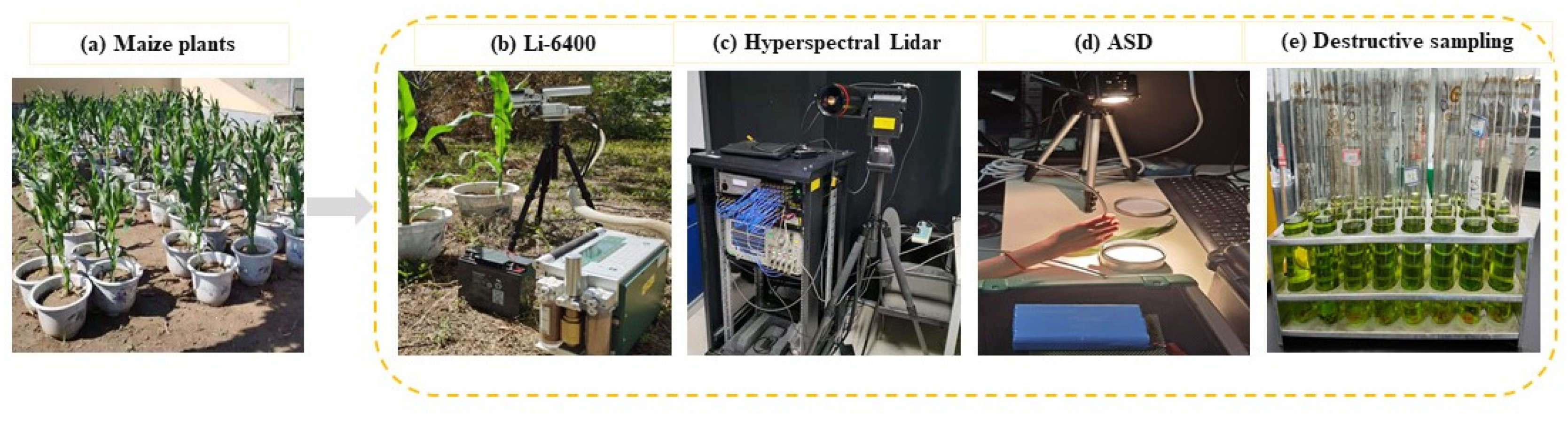
CO2 response curves were measured in situ when maize plants were under normal growth status. A portable leaf gas exchange system (LI-6400, LICOR Biosciences, Lincoln, NE, USA) was used. A standard 2 × 3 cm2 chamber with a red/blue LED light source was installed on the LI-6400 system, as shown in Figure 1b. The photosynthetic photon flux density was set at 2000 μmol m−1 s−1 to provide the light source for leaves, the temperature was set to close to the environment. Each maize leaf was first adapted to the environment of the chamber for about 30 min. During the measurement, the CO2 concentration in the chamber was set to 400, 300, 200, 100, 50, 400, 600, 800, 1000, 1200 μmol mol−1, and the measurement under each CO2 concentration lasted a minimum of 200 s and a maximum of 300 s. Vcmax and J at 25 °C were determined from measured CO2 response curves using a curve-fitting program for C4 plants [49].
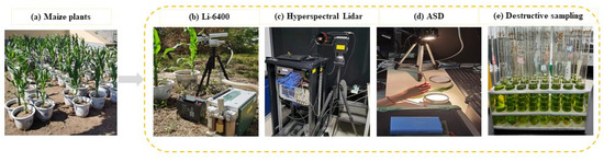
Figure 1.
The data collection of (a) potted maize plants, (b) Li-6400 measurement, (c) HSL scanning, (d) ASD measurement, and (e) destructive sampling.
2.3.2. HSL Data
Following the measurement of CO2 response curves, selected leaves were removed from maize plants and sent to the dark laboratory for HSL measurements. No external light was used since HSL actively emits the laser source. Before scanning each leaf, a white reference panel was scanned at a distance of 5 m. Subsequently, maize leaf pasted on a black panel and perpendicular to the laser source was scanned at the same distance. Twenty-five reflectance curves were recorded and then averaged to give the reflectance characteristics of each leaf.
Besides the acquisition of leaf-level HSL data, two maize plants inclined to the HSL system were scanned to further test the ability of HSL in characterizing 3D photosynthetic parameters. To correct the angle effect of backscatter intensity, another 10 maize leaves were scanned to simulate the fraction of specular and diffuse intensity. The incident angles varied between 0° and 70°, with a step of 5° from 0° to 30° and 10° from 30° to 70°.
For each full-waveform data, the backscattered intensity was defined as the maximum intensity of each curve after Gaussian filtering. The corresponding returned time was used to calculate line-of-sight distance based on the time-of-flight principle (distance = 3 ∗ 108 m/s ∗ returned time/2), thus the 3D position of each target point can be determined when coupled with the viewing angle. The reflectance at different wavelengths was defined as the ratio of backscattered intensity between the leaf and the white reference panel.
2.3.3. ASD Reflectance Data
Along with the HSL measurements, leaf reflectance was measured indoors using ASD with a spectral resolution of 1 nm (350–2500 nm). An illuminator was obliquely placed about 50 cm above targets to provide the external light for the ASD system. Other light sources were turned off during the measurement. Before measuring each leaf, the reflectance information of the reference panel was recorded. Twenty reflectance spectrums were measured at different positions for each leaf. Abnormal spectrums were eliminated based on the 3σ principle, and the remaining spectrums were averaged to give a mean value for each leaf.
2.3.4. Destructive Sampling
The determination of biochemical parameters was the last step. Measured leaves were placed in a plastic bag and then used for the determination of N and chlorophyll. When maize leaves were mixed in 95% ethanol, chlorophyll content was determined based on their absorption properties at two spectral bands (665 nm and 649 nm). The N concentration was subsequently determined using the Kjeldahl method [50]. Maize leaves were first oven-dried at 105 °C until a constant weight was reached and subsequently digested in a solution at 420 °C for 45 min in an automatic Kjeldahl digestion unit.
2.4. Incident Angle Correction
The specular backscattered intensity confounds the reflectance properties of targets, and the fraction of diffuse and specular intensity relies on both leaf surface and wavelength bands [51]. A linear combination of the Lambertian model and the Beckmann law [52] was used to simulate leaf backscattered intensity.
where is the backscatter intensity, is backscatter intensity at normal incidence angle, is the diffuse fraction and varies between 0 to 1, is incidence angle, and is the surface roughness and varies between 0 to 0.6.
and were determined when the best fit was observed between modeled and measured intensity via the iteration process. Leaf points with their incident angle above 70 degrees were removed from the maize point cloud, as the over-correction effect was observed for large incident angles [53].
2.5. Statistical Analysis
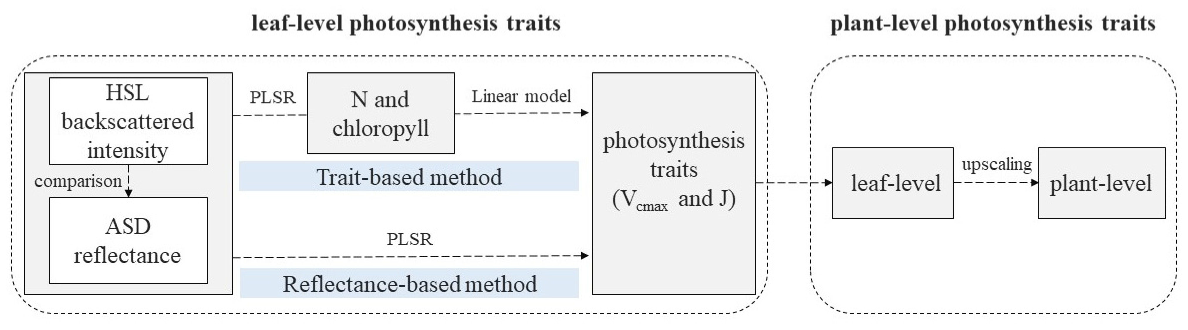
The workflow of this study is illustrated in Figure 2. Actual photosynthetic traits (e.g., Vcmax and J) of maize leaves were detected by the Li-6400 system, the spectral information of HSL was subsequently utilized for estimating these two photosynthesis traits. Given that the detection mechanisms between active and passive sensors differed, the result of HSL was also compared with that of the ASD at the leaf level. The estimation process was based on two methods: (1) Reflectance-based method [8,19,22]: partial least squares regression (PLSR) models of Vcmax and J were directly performed on all recorded spectral information; (2) trait-based method [19,54]: photosynthetic parameters were estimated based on their linear relationship with biochemical traits (N and chlorophyll), where the actual values of N and chlorophyll were obtained by destructive sampling. Compared with ASD, HSL can also extract spatial information of targets, achieving the simultaneous extraction of structural and spectral properties. Thus, with the correction of the incident angle effect in the HSL 3D point, the spatial distribution of photosynthetic traits at the plant level was characterized based on the constructed leaf-level estimating models.
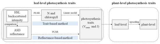
Figure 2.
Workflow of data processing.
The minimum root mean square errors of prediction (RMSEP) calculated from the validation results were utilized to determine the optimal number of latent variables. Due to the relatively small dataset of this research, no additional validation dataset but leave-one-out cross-validation method was used to test the prediction performance of constructed PLSR models. The coefficient of determination (R2), root mean square error (RMSE), and index of agreement (dr) were used to describe the fitness between measured and predicted values. dr was found to have a broad utility in model performance [55], its calculation was based on the mean absolute error (MAE) of estimation results and the mean absolute deviation (MAD) of observed values, as shown in Equation (2). For simplicity, we set c as 1.0. All statistical analyses were performed in Python, version 2.7 (http://www.python.org, accessed on 23 September 2021).
3. Results
3.1. Measured Leaf Properties
3.1.1. Leaf Traits
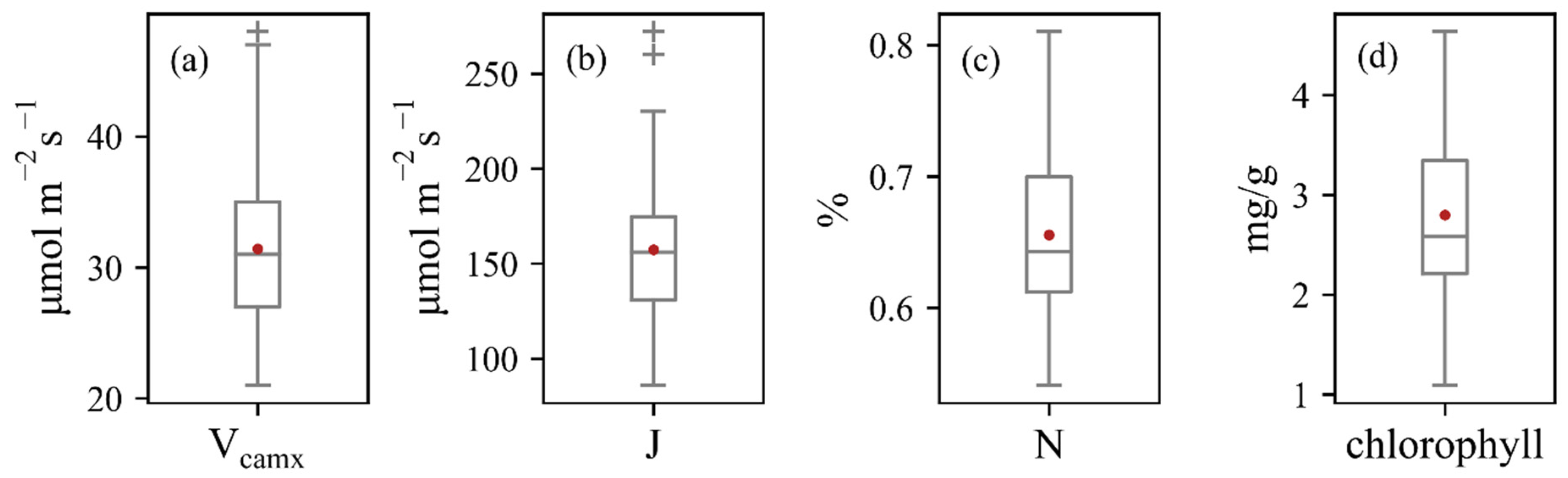
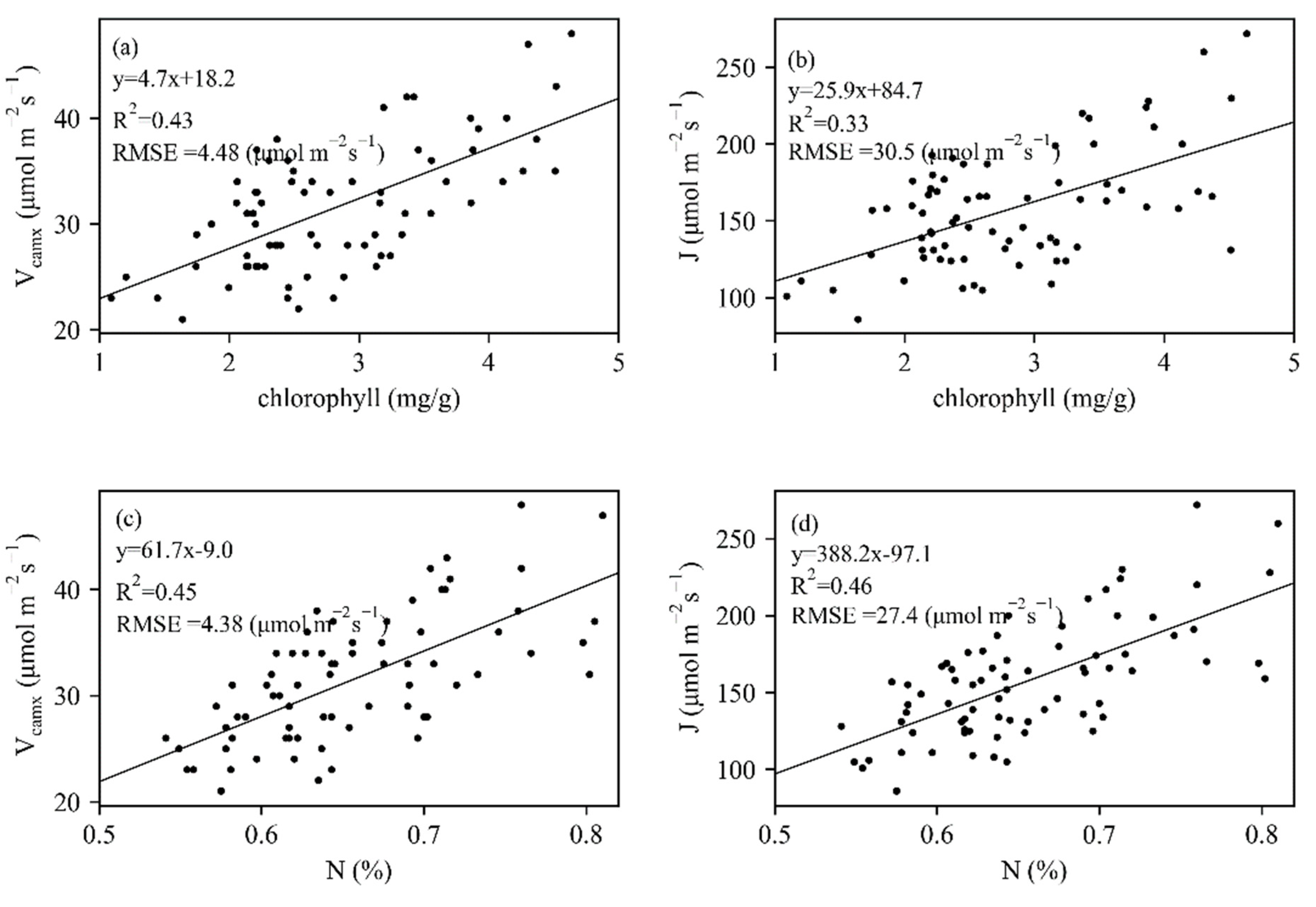
Measured leaf traits of 74 maize leaves collected from 50 maize plants presented a wide variation (Figure 3). Vcmax and J varied between 21 and 48 μmol m−2 s−1, 86 and 272 μmol m−2 s−1, respectively. Measured chlorophyll and N had close correlations with Vcmax and J (Figure 4), whereas N showed stronger relationships with photosynthesis traits. The constructed linear relationships were coupled with reflectance information for the trait-based estimation of Vcmax and J.

Figure 3.
Box plots of the measured values of (a) Vcmax, (b) J, (c) N, and (d) chlorophyll.
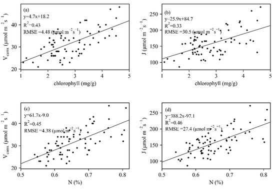
Figure 4.
The relationships between biochemical parameters (chlorophyll and N) and (a,c) Vcamx and (b,d) J.
3.1.2. Leaf Reflectance Spectra
The reflectance spectra (523–833 nm) were mainly located in the visible region, with several wavelengths belonging to the near-infrared region.
Twenty wavelength bands were contained in each HSL and ASD reflectance curve since ASD data was resampled according to HSL wavelengths. The spectral spectrums derived from passive and active sensors were slightly different, and the ASD spectrum was regarded as the leaf standard reflectance curve. The red-edge region of the HSL spectrum was not as steep as that of ASD, and the HSL reflectance was lower than ASD reflectance for wavelengths above 735 nm (Figure 5).
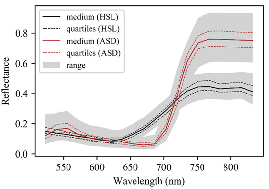
Figure 5.
Overview of leaf reflectance spectrum of 74 leaf samples measured by HSL and ASD system. The continuous black line stands for the median reflectance spectrum, the dashed red line stands for the first or third quartile reflectance spectrum, and the grey shaded area stands for the range of all reflectance spectrum.
3.2. Leaf-Level Photosynthesis Traits Estimation
3.2.1. Reflectance-Based Method
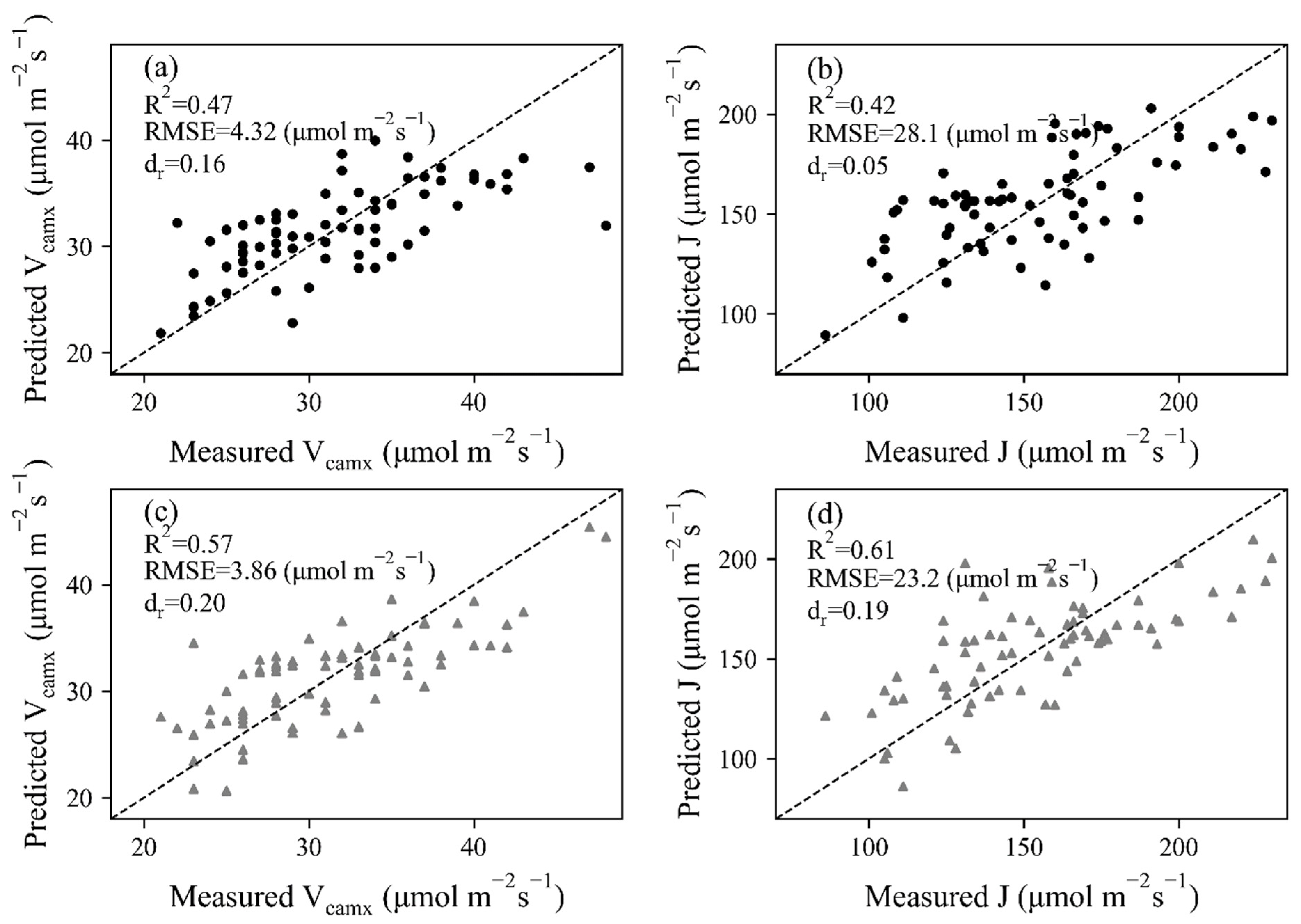
With reflectance at 20 wavelength bands as inputs, PLSR models of Vcmax and J were built by extracting principal components in these wavelengths. Leave-one-out cross-validation was conducted to show the estimating ability of constructed PLSR models, as shown in Figure 6. A moderate result (R2 = 0.47 and RMSE = 4.32 μmol mol−1 s−1 for Vcmax, R2 = 0.42 and RMSE = 28.1 μmol mol−1 s−1 for J) was observed for HSL data pairs. The dr value was largest (0.20) in J estimation with ASD data, indicating 20 percent of the total reference effort can be explained by model predictions. However, the two points with Vcmax higher than 43 μmol mol−1 s−1 obviously deviated from the 1:1 line.
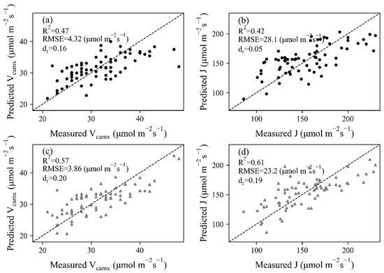
Figure 6.
Leave-one-out cross-validation results of Vcmax and J for (a,b) HSL and (c,d) ASD dataset. The dashed lines stand for 1:1 lines.
Compared with the results derived from the HSL dataset, improved relationships (R2 = 0.57 and 0.61 and RMSE = 3.86 μmol mol−1 s−1 for Vcmax, R2 = 0.61 and RMSE = 23.2 μmol mol−1 s−1 for J) were built between measured and predicted photosynthetic parameters for ASD data, and the data points of both Vcmax and J were closer to the 1:1 line. The main reason was that the leaf reflectance obtained by the commercial ASD system was more representative of leaf properties, despite an additional illumination that was needed during ASD data collection.
3.2.2. Trait-Based Method
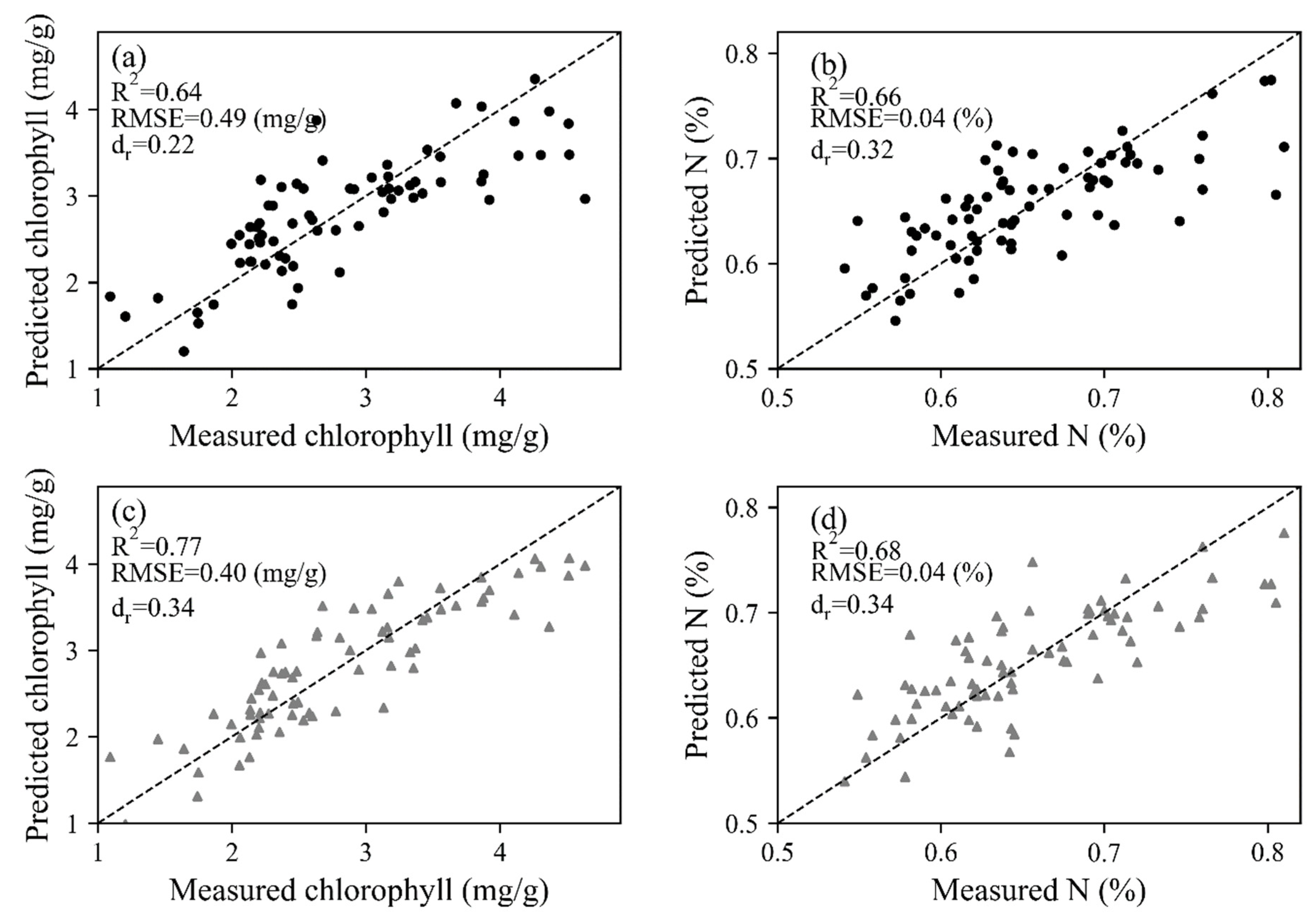
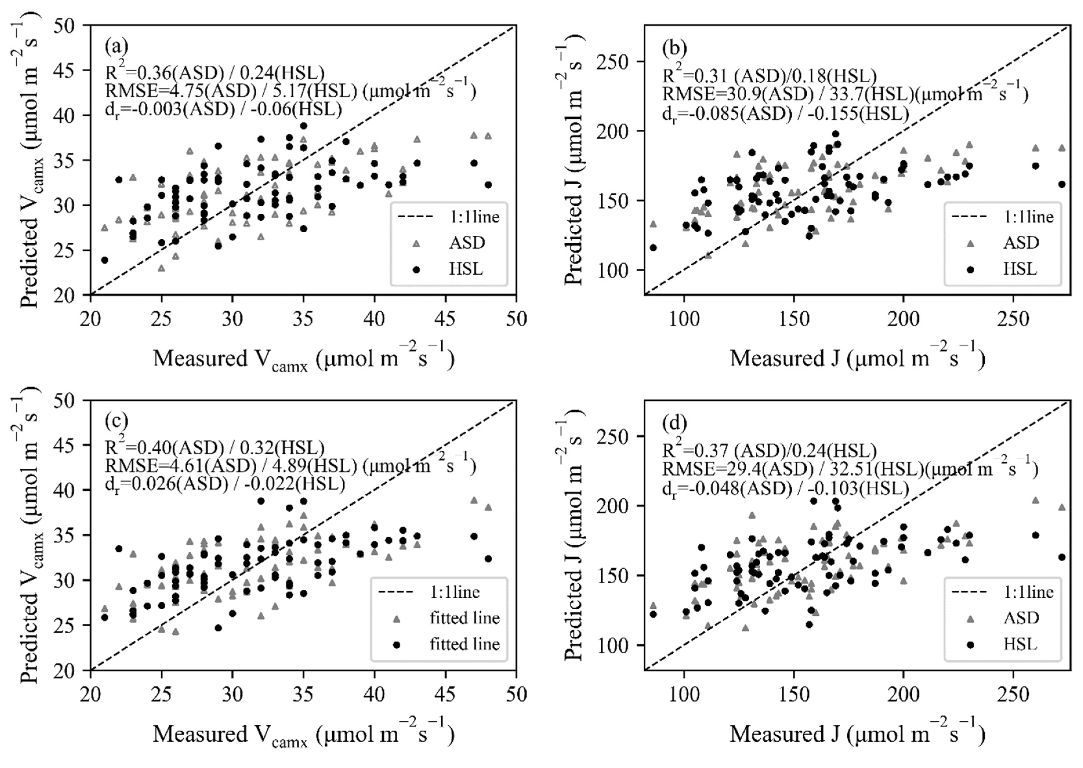
The trait-based method was based on the relationship between photosynthetic and biochemical parameters, thus the retrieval of chlorophyll and N using spectral information was the prerequisite. With the coefficients of constructed PLSR models, leave-one-out cross-validation results were obtained by leaving one sample as the testing dataset for each repetition (Figure 7). The dr values were all located in the positive portion, varying between 0.22 and 0.68. For both HSL and ASD datasets, the correlation between measured and predicted values was better for chlorophyll (R2 = 0.64 for HSL and 0.77 for ASD) than N concentration (R2 = 0.66 for HSL and 0.68 for ASD), and the estimation accuracy of biochemical properties was higher in contrast with photosynthetic parameters. With the estimated chlorophyll and N values, as well as the constructed linear model between biochemical and photosynthetic parameters (Figure 4), Vcamx and J were predicted and then fitted with measured values (Figure 8). Most dr values were negative, which means that the average error magnitude was larger than the average reference error. The data points of ASD were closer to the 1:1 line, thus higher R2 (R2 ≥ 0.32 for Vcamx and ≥0.24 for J) and lower RMSE values (RMSE ≤ 4.89 μmol mol−1 s−1 for Vcamx and ≤32.51 μmol mol−1 s−1 for J) were obtained than HSL data. The N-based method (Figure 8a,b) performed better than the chlorophyll-based method (Figure 8c,d).

Figure 7.
Leave-one-out cross-validation results of chlorophyll and N for (a,b) HSL and (c,d) ASD dataset. The dashed lines stand for 1:1 lines.
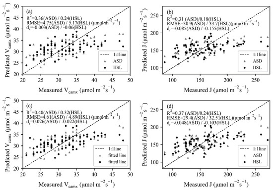
Figure 8.
The relationships between measured and estimated Vcmax and J using (a,b) chlorophyll-based method and (c,d) N-based method for HSL and ASD data.
Leaf spectrum contained more information about biochemical properties than Vcmax and J, and corresponding PLSR models with higher accuracy were constructed for chlorophyll and N concentration. However, the trait-based method showed weaker estimation ability than the reflectance-based method (Table 2) since the highest relationship in Vmax or J estimation was obtained by using the reflectance-based method for both ASD and HSL datasets. Data points of the trait-based method were far away from the 1:1 line, especially for Vcamx and J with higher values. This was mainly caused by the weaker correlation between measured biochemical and photosynthetic parameters of the experimental dataset.
Table 2.
The R2 values of Vcmax and J estimation results for HSL and ASD datasets. The highest R2 values are shown in bold.
3.3. Plant-Level Photosynthesis Traits Characterization
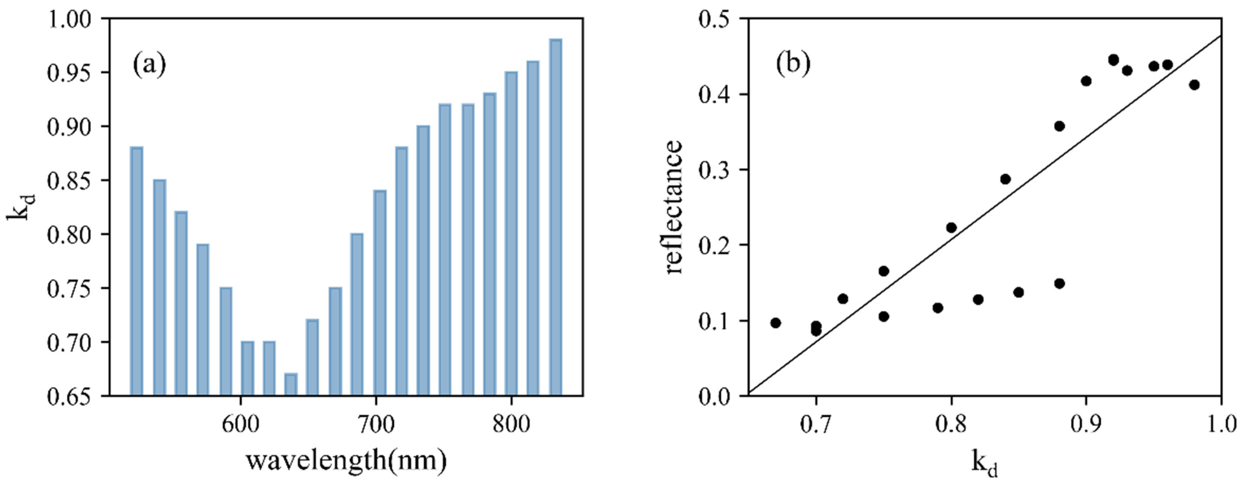
The diffuse fraction and the roughness at different wavelengths were retrieved from the Lambertian–Beckmann simulating model (Table 3). The constructed models, with R2 all above 0.74, performed well for simulating the reflectance of maize leaves at different incident angles. With the increasing wavelengths, kd values decreased in the first few bands and then significantly increased from 637 nm (Figure 9a). To further explore the relationship between the faction of diffuse intensity and reflectance at 20 wavelength bands, a linear model was built and a strong positive correlation (R2 = 0.77, Figure 9b) was observed. The four points within 523–572 nm deviated from others, which was related to lidar manufacturing technology. In contrast, m showed no dependence on wavelengths. Constructed Lambertian–Beckmann models were subsequently utilized for correcting the angle effect of the maize 3D point cloud.
Table 3.
The simulation of HSL backscattered intensity based on the linear combination of Lambertian model and Beckmann law. kd stands for the diffuse fraction, and m stands for surface roughness.
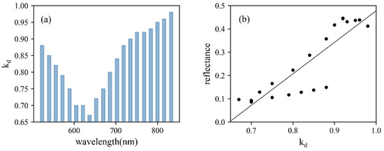
Figure 9.
(a) The diffuse fraction, kd, of constructed Lambertian–Beckmann models. (b) The linear relationship between kd and reflectance of 20 wavelength bands.
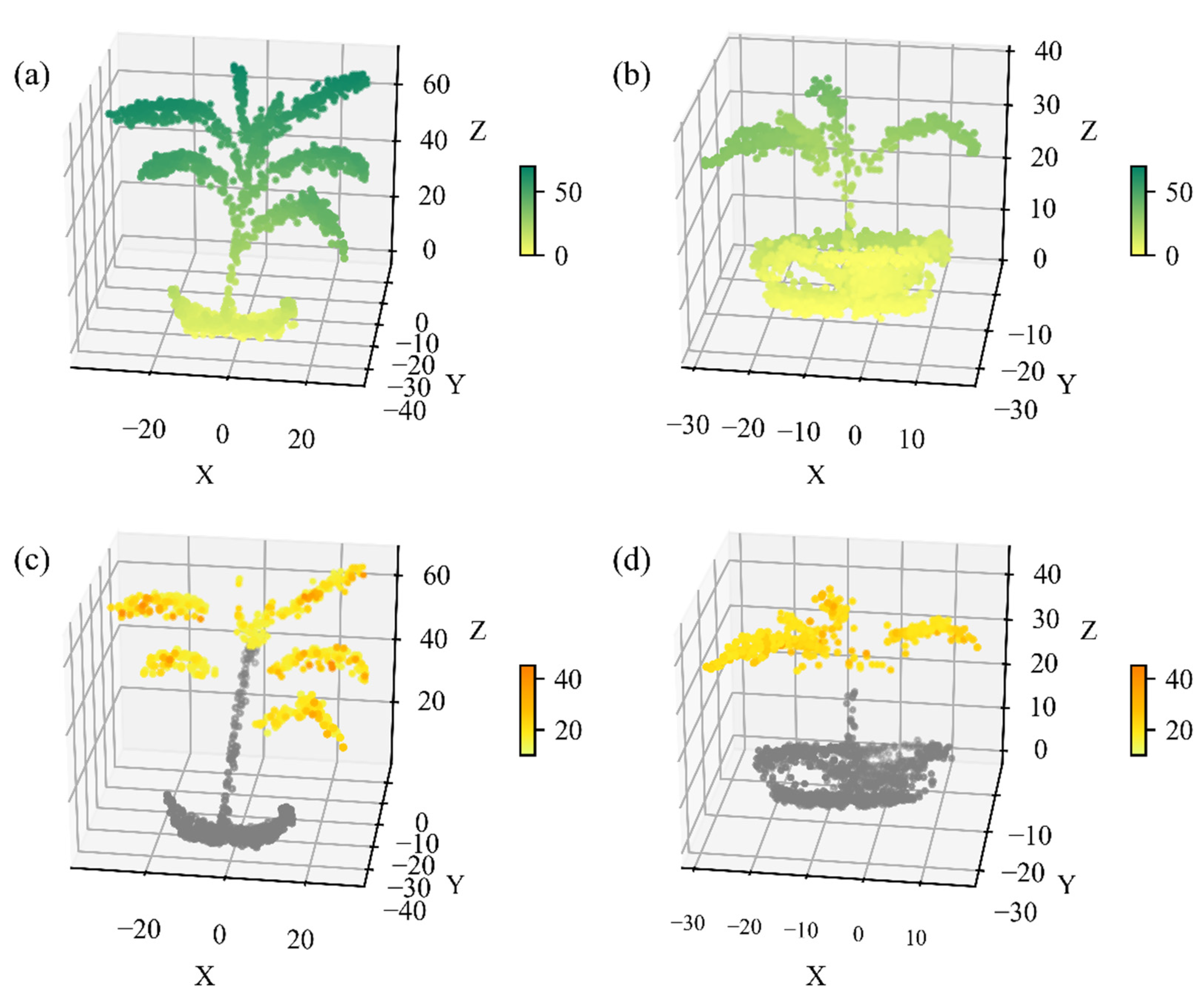
The spectral point cloud of two maize plants was constructed from HSL full-waveform data. The spatial property of maize plants was visually demonstrated in Figure 10a,b. The maize leaves and stem were separated and displayed in space, despite the density of the maize point cloud being relatively sparse which was limited by the scanning speed of the HSL prototype system. Leaf points with their incident angle below 70 degrees were further used for calculating photosynthetic parameters, while the spectral information of stem and flowerpot points were not processed. Taking Vcmax as an example, the 3D distribution of photosynthetic parameters, estimated using the reference-based method, was subsequently characterized based on the spectral information at each position (Figure 10c,d), demonstrating the potential ability of HSL to monitor plant photosynthesis in 3D space.
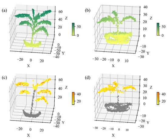
Figure 10.
The 3D distribution of (a,b) elevation and (c,d) Vcmax of two potted maize plants. The units of elevation and Vcmax were cm and μmol mol−1 s−1, respectively. Vcmax values were estimated using the constructed PLSR model of the reflectance-based method. The unit of X, Y, and Z was centimeter.
4. Discussion
Previous studies have tested the ability of passive optical sensors in plant photosynthesis traits estimation [8,19,22], while these remote sensors were easily affected by some confounding factors (e.g., illuminating conditions, plant structure, and soil background) and had a weak ability in detecting plant structural parameters, limiting their further application in precision agriculture. In contrast, this study showed the potential of HSL as an active remote sensor in estimating maize photosynthesis properties at both the leaf level and plant level. The estimation accuracy of HSL (R2 < 0.5) was lower than that of previous studies conducted with passive spectral data [19,20,22], which can be explained by several points: (1) The high intensity of the HSL laser beam and ASD illuminator caused damage to leaf physiological properties, thus leaf spectral properties were slightly changed; (2) except for Li-6400 measurements conducted in situ with living leaves, other measurements were carried out with maize leaves removed from maize plants; (3) only 20 wavelength bands with a higher signal-to-noise ratio (523–833 nm) were chosen in this experiment, while previous researchers used more wavelength bands with a wider spectral range. The collected spectral spectrum of ASD and HSL was not identical (Figure 5), which can be explained by the difference in measurement time between these two systems and the different detection mechanisms between active and passive remote sensors. Compared with the estimation results of HSL, ASD showed a higher accuracy at the 2D leaf level (Table 2). However, ASD as a passive optical sensor needs an external light source and has a weak ability in characterizing plant 3D structural properties. In contrast, with the ability to generate a 3D spectral point cloud, HSL as an active sensor can characterize photosynthesis traits at the plant level.
Leaf traits (e.g., chlorophyll, N, and LMA) have been proven to have a strong linkage with photosynthetic parameters [8,20,22]. Chlorophyll, N, Vcmax, and J of maize leaves were simultaneously estimated by HSL (Figure 6 and Figure 8), thus the reflectance information can provide an insight into the mechanism under photosynthesis prediction. The reflectance-based method performed better than the N-based method and chlorophyll-based method (Table 2), while the result of this study was not consistent with previous studies demonstrating that the trait-based method was superior to the reflectance-based method [19]. In this study, HSL reflectance information had a closer relationship with biochemical parameters than photosynthesis traits, while the weaker relationship between measured biochemical and photosynthetic data (Figure 4) caused the lower accuracy of the trait-based method.
The diffuse fraction of backscattered intensity comes from the multiple scattering of leaf radiation, and the intensity of specular reflection represents the properties of the leaf surface [52]. In this study, the linear combination of the Beckmann law and the Lambertian model was used for the correction of the incident angle. With R2 ranging from 0.74 to 0.92 at 20 wavelengths (Table 3), this simulating model showed its effectiveness for lidar data, the same as previous lidar studies [52]. The diffuse fraction, kd, of constructed simulating models showed a strong dependence on wavelength bands, where the wavelength with a higher reflectance had a higher kd value (Figure 9). The wavelength-dependent feature of the specular and diffuse fraction was also observed by Qian et al. [56].
Plant photosynthesis is not only related to photosynthetic parameters such as Vcmax, and J, but also to light interception largely affected by canopy structure [9,57]. Prior to the simulation of light interception within the plant canopy using optical simulating methods such as ray-tracing and radiosity, the accurate construction of plant 3D models is vitally important [10,57,58]. Lidar systems have a strong ability in constructing 3D point clouds, and HSL prototype systems have shown their ability in the extraction of structural parameters [59,60,61]. Thus, HSL has the potential to assess canopy light interception when coupled with optical simulating models. In this study, the spatial distribution of Vcmax of two maize plants was illustrated based on the HSL point cloud (Figure 10).
Several limitations were faced in this study that requires improvements in further studies. Firstly, the HSL used in this study was a prototype system, thus its scanning efficiency was inferior compared with commercial lidar devices. To meet the requirement of obtaining a large dataset, the development of hardware manufacturing technology is the prerequisite. Secondly, the maximum returned intensity of 20 wavelength bands was extracted after the Gaussian filtering of full-waveform data in this experiment, whereas more data processing methods need to be explored as the HSL data containing both spectral and spatial information is a novel type of lidar data.
Furthermore, the experiment was performed indoors and mounted on a tripod. High-throughput plant phenotyping platforms aimed at improving the data collection efficiency and accuracy, thus the efficiency of crop breeding, involves various proximal sensing platforms and remote sensing platforms [1,62]. Lidar sensors can be boarded on proximal sensing planforms (e.g., gantry, vehicle, tripod, backpack, and handheld platforms) both indoors and outdoors [62], while the efficiency of some field-based platforms is limited when applied to large plot areas [63]. For remote sensing platforms, laser sensors can couple with unmanned aerial vehicles, manned aircraft, and satellites for efficient high-throughput monitoring of plant phenotyping at the plot, landscape, or region level [64,65]. Despite the high-throughput measurement of photosynthesis traits not being possible with prototype HSL systems at present, HSL with improved manufacturing technology may board on various platforms to meet high-throughput demands of photosynthesis estimation in the future.
5. Conclusions
The results successfully addressed the three points evaluated in the study: (1) Based on the spectral information of 20 wavelength bands, HSL has the ability to estimate photosynthetic parameters. (2) The estimation accuracy of ASD was higher than that of HSL, as ASD was a commercial system while the efficiency of the prototype HSL system needs to be further improved. The estimation process was based on either the reference-based method or the trait-based method, whereas the trait-based method performed worse than the reflectance-based method for both ASD and HSL datasets (Table 2). (3) Containing spectral and structural properties of targets, HSL data have the ability to estimate photosynthesis traits at both the leaf level and 3D plant level.
The linear combination of the Lambertian model and Beckmann law performed well (R2 ≥ 0.74 for 20 wavelength bands) in correcting the incident angle, thus the distribution of plant-level photosynthesis traits was visually displayed based on the HSL 3D spectral point cloud. The characterization of 3D photosynthesis traits is beneficial for understanding the upscaling process of plant photosynthesis [5], estimating photosynthetic performance at larger scales [3], and optimizing crop-simulating models [4]. Despite the potential of HSL in estimating 3D photosynthesis traits not being fully explored, this study provided the basis for further application of HSL in the photosynthesis field.
The maximum returned intensity of HSL full-waveform was used for the estimation of maize biochemical and photosynthetic properties; whereas, full-waveform data is superior to discrete returns, as it can extract more information (e.g., echo width and backscatter cross-section) correlated with plant reflectance information [66,67]. In the next step, the advanced data decomposition method of HSL full-waveform data needs to be explored. With the development of HSL hardware manufacturing technology, HSL could be boarded on various platforms for high-throughput measurement of plant photosynthesis, which is important for breeding studies and the pursuit of crop yield.
Author Contributions
Conceptualization, S.G.; methodology, K.B. and S.X.; software, Z.H.; validation, S.G. and Z.N.; formal analysis, J.B.; investigation, J.B. and G.S.; resources, Z.N. and G.S.; data curation, J.B.; writing—original draft preparation, K.B. and S.X.; writing—review and editing, K.B. and S.X.; visualization, J.W.; supervision, S.G.; project administration, S.G.; funding acquisition, S.G. and Z.N. All authors have read and agreed to the published version of the manuscript.
Funding
The study was funded by National Natural Science Foundation of China (41730107), National Natural Science Foundation of China (42171377) and the Strategic Priority Research Program of Chinese Academy of Sciences (XDA19030304).
Acknowledgments
The authors wish to express heartfelt thanks to the researchers of the National Experiment Station for Precision Agriculture for providing us with potted maize plants. We greatly appreciate the constructive comments from the all anonymous reviewers.
Conflicts of Interest
The authors declare no conflict of interest.
References
- Zhao, C.; Zhang, Y.; Du, J.; Guo, X.; Wen, W.; Gu, S.; Wang, J.; Fan, J. Crop phenomics: Current status and perspectives. Front. Plant Sci. 2019, 10, 714. [Google Scholar] [CrossRef] [Green Version]
- Ray, D.K.; Mueller, N.D.; West, P.C.; Foley, J.A. Yield trends are insufficient to double global crop production by 2050. PLoS ONE 2013, 8, e66428. [Google Scholar] [CrossRef] [Green Version]
- Meacham-Hensold, K.; Fo, P.; Wu, J.; Serbin, S.; Montes, C.C.; Ainsworth, E.; Guan, K.; Dracup, E.; Pederson, T.; Driever, S.; et al. Plot-level rapid screening for photosynthetic parametersusing proximal hyperspectral imaging. J. Exp. Bot. 2020, 71, 2312–2328. [Google Scholar] [CrossRef]
- Chang, T.-G.; Zhao, H.; Wang, N.; Song, Q.-F.; Xiao, Y.; Qu, M.; Zhu, X.-G. A three-dimensional canopy photosynthesis model in rice with a complete description of the canopy architecture, leaf physiology, and mechanical properties. J. Exp. Bot. 2019, 70, 2479–2490. [Google Scholar] [CrossRef]
- Wu, A.; Song, Y.; van Oosterom, E.J.; Hammer, G.L. Connecting biochemical photosynthesis models with crop models to support crop improvement. Front. Plant Sci. 2016, 7, 1518. [Google Scholar] [CrossRef] [Green Version]
- Long, S.P.; Marshall-Colon, A.; Zhu, X.G. Meeting the global food demand of the future by engineering crop photosynthesis and yield potential. Cell 2015, 161, 56–66. [Google Scholar] [CrossRef] [PubMed] [Green Version]
- Furbank, R.T.; Tester, M. Phenomics--technologies to relieve the phenotyping bottleneck. Trends Plant Sci. 2011, 16, 635–644. [Google Scholar] [CrossRef] [PubMed]
- Meacham-Hensold, K.; Montes, C.M.; Wu, J.; Guan, K.; Fu, P.; Ainsworth, E.A.; Pederson, T.; Moore, C.E.; Brown, K.L.; Raines, C.; et al. High-throughput field phenotyping using hyperspectral reflectance and partial least squares regression (PLSR) reveals genetic modifications to photosynthetic capacity. Remote Sens. Environ. 2019, 231, 111176. [Google Scholar] [CrossRef] [PubMed]
- Niinemets, U. Photosynthesis and resource distribution through plant canopies. Plant Cell Environ. 2007, 30, 1052–1071. [Google Scholar] [CrossRef] [PubMed]
- Kim, D.; Kang, W.H.; Hwang, I.; Kim, J.; Kim, J.H.; Park, K.S.; Son, J.E. Use of structurally-accurate 3D plant models for estimating light interception and photosynthesis of sweet pepper (Capsicum annuum) plants. Comput. Electron. Agric. 2020, 177, 105689. [Google Scholar] [CrossRef]
- Hirose, T. Development of the monsi-saeki theory on canopy structure and function. In Annals of Botany; Oxford University Press: London, UK, 2005. [Google Scholar]
- Fu, P.; Meacham-Hensold, K.; Siebers, M.H.; Bernacchi, C.J. The inverse relationship between solar-induced fluorescence yield and photosynthetic capacity: Benefits for field phenotyping. J. Exp. Bot. 2020, 72, 1295–1306. [Google Scholar] [CrossRef] [PubMed]
- Porcar-Castell, A.; Tyystjarvi, E.; Atherton, J.; van der Tol, C.; Flexas, J.; Pfundel, E.E.; Moreno, J.; Frankenberg, C.; Berry, J.A. Linking chlorophyll a fluorescence to photosynthesis for remote sensing applications: Mechanisms and challenges. J. Exp. Bot. 2014, 65, 4065–4095. [Google Scholar] [CrossRef] [PubMed]
- Yang, H.; Yang, X.; Zhang, Y.; Heskel, M.A.; Lu, X.; Munger, J.W.; Sun, S.; Tang, J. Chlorophyll fluorescence tracks seasonal variations of photosynthesis from leaf to canopy in a temperate forest. Glob. Chang. Biol. 2017, 23, 2874–2886. [Google Scholar] [CrossRef] [PubMed]
- Dechant, B.; Ryu, Y.; Badgley, G.; Zeng, Y.; Berry, J.A.; Zhang, Y.; Goulas, Y.; Li, Z.; Zhang, Q.; Kang, M.; et al. Canopy structure explains the relationship between photosynthesis and sun-induced chlorophyll fluorescence in crops. Remote Sens. Environ. 2020, 241, 111733. [Google Scholar] [CrossRef] [Green Version]
- Lu, X.; Liu, Z.; Zhao, F.; Tang, J. Comparison of total emitted solar-induced chlorophyll fluorescence (SIF) and top-of-canopy (TOC) SIF in estimating photosynthesis. Remote Sens. Environ. 2020, 251, 112083. [Google Scholar] [CrossRef]
- Alonso, L.; Gomez-Chova, L.; Vila-Frances, J.; Amoros-Lopez, J.; Guanter, L.; Calpe, J.; Moreno, J. Improved fraunhofer line discrimination method for vegetation fluorescence quantification. IEEE Geosci. Remote Sens. Lett. 2008, 5, 620–624. [Google Scholar] [CrossRef]
- Dechant, B.; Ryu, Y.; Kang, M. Making full use of hyperspectral data for gross primary productivity estimation with multivariate regression: Mechanistic insights from observations and process-based simulations. Remote Sens. Environ. 2019, 234, 111435. [Google Scholar] [CrossRef]
- Dechant, B.; Cuntz, M.; Vohland, M.; Schulz, E.; Doktor, D. Estimation of photosynthesis traits from leaf reflectance spectra: Correlation to nitrogen content as the dominant mechanism. Remote Sens. Environ. 2017, 196, 279–292. [Google Scholar] [CrossRef]
- Wang, S.; Guan, K.; Wang, Z.; Ainsworth, E.A.; Zheng, T.; Townsend, P.A.; Li, K.; Moller, C.; Wu, G.; Jiang, C. Unique contributions of chlorophyll and nitrogen to predict crop photosynthetic capacity from leaf spectroscopy. J. Exp. Bot. 2020, 72, 341–354. [Google Scholar] [CrossRef] [PubMed]
- Serbin, S.P.; Dillaway, D.N.; Kruger, E.L.; Townsend, P.A. Leaf optical properties reflect variation in photosynthetic metabolism and its sensitivity to temperature. J. Exp. Bot. 2012, 63, 489–502. [Google Scholar] [CrossRef] [Green Version]
- Yendrek, C.R.; Tomaz, T.; Montes, C.M.; Cao, Y.; Morse, A.M.; Brown, P.J.; McIntyre, L.M.; Leakey, A.D.; Ainsworth, E.A. High-throughput phenotyping of maize leaf physiological and biochemical traits using hyperspectral reflectance. Plant Physiol. 2017, 173, 614–626. [Google Scholar] [CrossRef]
- Silva-Perez, V.; Molero, G.; Serbin, S.P.; Condon, A.G.; Reynolds, M.P.; Furbank, R.T.; Evans, J.R. Hyperspectral reflectance as a tool to measure biochemical and physiological traits in wheat. J. Exp. Bot. 2018, 69, 483–496. [Google Scholar] [CrossRef] [PubMed] [Green Version]
- Jiang, Y.; Snider, J.L.; Li, C.; Rains, G.C.; Paterson, A.H. Ground based hyperspectral imaging to characterize canopy-level photosynthetic activities. Remote Sens. 2020, 12, 315. [Google Scholar] [CrossRef] [Green Version]
- Watt, M.S.; Buddenbaum, H.; Leonardo, E.M.C.; Estarija, H.J.C.; Bown, H.E.; Gomez-Gallego, M.; Hartley, R.; Massam, P.; Wright, L.; Zarco-Tejada, P.J. Using hyperspectral plant traits linked to photosynthetic efficiency to assess N and P partition. ISPRS J. Photogramm. Remote Sens. 2020, 169, 406–420. [Google Scholar] [CrossRef]
- Serbin, S.P.; Singh, A.; Desai, A.R.; Dubois, S.G.; Jablonski, A.D.; Kingdon, C.C.; Kruger, E.L.; Townsend, P.A. Remotely estimating photosynthetic capacity, and its response to temperature, in vegetation canopies using imaging spectroscopy. Remote Sens. Environ. 2015, 167, 78–87. [Google Scholar] [CrossRef]
- Behmann, J.; Mahlein, A.-K.; Paulus, S.; Kuhlmann, H.; Oerke, E.-C.; Plümer, L. Calibration of hyperspectral close-range pushbroom cameras for plant phenotyping. ISPRS J. Photogramm. Remote Sens. 2015, 106, 172–182. [Google Scholar] [CrossRef]
- Eitel, J.U.H.; Höfle, B.; Vierling, L.A.; Abellán, A.; Asner, G.P.; Deems, J.S.; Glennie, C.L.; Joerg, P.C.; LeWinter, A.L.; Magney, T.S.; et al. Beyond 3-D: The new spectrum of lidar applications for earth and ecological sciences. Remote Sens. Environ. 2016, 186, 372–392. [Google Scholar] [CrossRef] [Green Version]
- Liu, H.; Bruning, B.; Garnett, T.; Berger, B. Hyperspectral imaging and 3D technologies for plant phenotyping: From satellite to close-range sensing. Comput. Electron. Agric. 2020, 175, 105621. [Google Scholar] [CrossRef]
- Lv, Y.; Xu, J.; Liu, X.; Wang, H. Vertical profile of photosynthetic light response within rice canopy. Int. J. Biometeorol. 2020, 64, 1699–1708. [Google Scholar] [CrossRef] [PubMed]
- Behmann, J.; Mahlein, A.-K.; Paulus, S.; Dupuis, J.; Kuhlmann, H.; Oerke, E.-C.; Plümer, L. Generation and application of hyperspectral 3D plant models: Methods and challenges. Mach. Vis. Appl. 2015, 27, 611–624. [Google Scholar] [CrossRef]
- Budei, B.C.; St-Onge, B.; Hopkinson, C.; Audet, F.-A. Identifying the genus or species of individual trees using a three-wavelength airborne lidar system. Remote Sens. Environ. 2017, 204, 632–647. [Google Scholar] [CrossRef]
- Pan, S.; Guan, H.; Chen, Y.; Yu, Y.; Gonçalves, W.N.; Marcato Junior, J.; Li, J. Land-cover classification of multispectral LiDAR data using CNN with optimized hyper-parameters. ISPRS J. Photogramm. Remote Sens. 2020, 166, 241–254. [Google Scholar] [CrossRef]
- Aasen, H.; Burkart, A.; Bolten, A.; Bareth, G. Generating 3D hyperspectral information with lightweight UAV snapshot cameras for vegetation monitoring: From camera calibration to quality assurance. ISPRS J. Photogramm. Remote Sens. 2015, 108, 245–259. [Google Scholar] [CrossRef]
- Renhorn, I.; Bergström, D.; Hedborg, J.; Letalick, D.; Möller, S. High spatial resolution hyperspectral camera based on a linear variable filter. Opt. Eng. 2016, 55, 114105. [Google Scholar] [CrossRef] [Green Version]
- Chen, Y.; Raikkonen, E.; Kaasalainen, S.; Suomalainen, J.; Hakala, T.; Hyyppa, J.; Chen, R. Two-channel hyperspectral LiDAR with a supercontinuum laser source. Sensors 2010, 10, 7057–7066. [Google Scholar] [CrossRef] [PubMed] [Green Version]
- Shao, H.; Chen, Y.; Yang, Z.; Jiang, C.; Li, W.; Wu, H.; Wen, Z.; Wang, S.; Puttnon, E.; Hyyppa, J. A 91-channel hyperspectral LiDAR for Coal/Rock classification. IEEE Geosci. Remote Sens. Lett. 2019, 17, 1052–1056. [Google Scholar] [CrossRef] [Green Version]
- Wei, G.; Shalei, S.; Bo, Z.; Shuo, S.; Faquan, L.; Xuewu, C. Multi-wavelength canopy LiDAR for remote sensing of vegetation: Design and system performance. ISPRS J. Photogramm. Remote Sens. 2012, 69, 1–9. [Google Scholar] [CrossRef]
- Niu, Z.; Xu, Z.; Sun, G.; Huang, W.; Wang, L.; Feng, M.; Li, W.; He, W.; Gao, S. Design of a new multispectral waveform LiDAR instrument to monitor vegetation. IEEE Geosci. Remote Sens. Lett. 2015, 12, 1506–1510. [Google Scholar] [CrossRef]
- Wang, Z.; Li, C.; Zhou, M.; Zhang, H.; He, W.; Li, W.; Qiu, Y. Recent development of hyperspectral LiDAR using supercontinuum laser. In Proceedings of the International Symposium on Optoelectronic Technology and Application, Beijing, China, 25 October 2016; p. 101560I. [Google Scholar]
- Sun, G.; Niu, Z.; Gao, S.; Huang, W.; Wang, L.; Li, W.; Feng, M. 32-channel hyperspectral waveform LiDAR instrument to monitor vegetation: Design and initial performance trials. In Proceedings of the SPIE—The International Society for Optical Engineering, Beijing, China, 18 November 2014; Volume 9263. [Google Scholar]
- Bi, K.; Xiao, S.; Gao, S.; Zhang, C.; Huang, N.; Niu, Z. Estimating vertical chlorophyll concentrations in maize in different health states using hyperspectral LiDAR. IEEE Trans. Geosci. Remote Sens. 2020, 58, 8125–8133. [Google Scholar] [CrossRef]
- Sun, J.; Shi, S.; Yang, J.; Chen, B.; Gong, W.; Du, L.; Mao, F.; Song, S. Estimating leaf chlorophyll status using hyperspectral lidar measurements by PROSPECT model inversion. Remote Sens. Environ. 2018, 212, 1–7. [Google Scholar] [CrossRef]
- Du, L.; Gong, W.; Shi, S.; Yang, J.; Sun, J.; Zhu, B.; Song, S. Estimation of rice leaf nitrogen contents based on hyperspectral LIDAR. Int. J. Appl. Earth Obs. Geoinf. 2016, 44, 136–143. [Google Scholar] [CrossRef]
- Nevalainen, O.; Hakala, T.; Suomalainen, J.; Mäkipää, R.; Peltoniemi, M.; Krooks, A.; Kaasalainen, S. Fast and nondestructive method for leaf level chlorophyll estimation using hyperspectral LiDAR. Agric. For. Meteorol. 2014, 198, 250–258. [Google Scholar] [CrossRef]
- Hakala, T.; Nevalainen, O.; Kaasalainen, S.; Mäkipää, R. Technical note: Multispectral lidar time series of pine canopy chlorophyll content. Biogeosciences 2015, 12, 1629–1634. [Google Scholar] [CrossRef] [Green Version]
- Lin, Y. LiDAR: An important tool for next-generation phenotyping technology of high potential for plant phenomics? Comput. Electron. Agric. 2015, 119, 61–73. [Google Scholar] [CrossRef]
- Su, Y.; Wu, F.; Ao, Z.; Jin, S.; Qin, F.; Liu, B.; Pang, S.; Liu, L.; Guo, Q. Evaluating maize phenotype dynamics under drought stress using terrestrial lidar. Plant Methods 2019, 15, 11. [Google Scholar] [CrossRef] [Green Version]
- Zhou, H.; Akçay, E.; Helliker, B.R. Estimating C4 photosynthesis parameters by fitting intensive A/Ci curves. Photosynth. Res. 2019, 141, 181–194. [Google Scholar] [CrossRef] [PubMed]
- Bradstreet, R.B. Kjeldahl method for organic nitrogen. Anal. Chem. 1954, 26, 185–187. [Google Scholar] [CrossRef]
- Kaasalainen, S.; Akerblom, M.; Nevalainen, O.; Hakala, T.; Kaasalainen, M. Uncertainty in multispectral lidar signals caused by incidence angle effects. Interface Focus 2018, 8, 20170033. [Google Scholar] [CrossRef] [PubMed] [Green Version]
- Zhu, X.; Wang, T.; Darvishzadeh, R.; Skidmore, A.K.; Niemann, K.O. 3D leaf water content mapping using terrestrial laser scanner backscatter intensity with radiometric correction. ISPRS J. Photogramm. Remote Sens. 2015, 110, 14–23. [Google Scholar] [CrossRef]
- Du, L.; Zhili, J.; Chen, B.; Chen, B.; Gao, W.; Yang, J.; Shi, S.; Song, S.; Wang, M.; Gong, W.; et al. Application of hyperspectral LiDAR on 3D chlorophyll-nitrogen mapping of Rohdea japonica in laboratory. IEEE J. Sel. Top. Appl. Earth Obs. Remote Sens. 2021, 14, 9667–9679. [Google Scholar] [CrossRef]
- Walker, A.P.; Beckerman, A.P.; Gu, L.; Kattge, J.; Cernusak, L.A. The relationship of leaf photosynthetic traits—Vcmax and Jmax -to leaf nitrogen, leaf phosphorus, and specific leaf area: A meta-analysis and modeling study. Ecol. Evol. 2014, 4, 3218–3235. [Google Scholar] [CrossRef] [Green Version]
- Willmott, C.J.; Robeson, S.M.; Matsuura, K.; Ficklin, D.L. Assessment of three dimensionless measures of model performance. Environ. Model. Softw. 2015, 73, 167–174. [Google Scholar] [CrossRef]
- Qian, X.; Yang, J.; Shi, S.; Gong, W.; Du, L.; Chen, B.; Chen, B. Analyzing the effect of incident angle on echo intensity acquired by hyperspectral lidar based on the Lambert-Beckman model. Opt. Express 2021, 29, 11055–11069. [Google Scholar] [CrossRef] [PubMed]
- Song, Q.; Zhang, G.; Zhu, X.G. Optimal crop canopy architecture to maximise canopy photosynthetic CO2 uptake under elevated CO2—A theoretical study using a mechanistic model of canopy photosynthesis. Funct. Plant Biol. 2013, 40, 108–124. [Google Scholar] [CrossRef] [PubMed] [Green Version]
- Kim, J.H.; Lee, J.W.; Ahn, T.I.; Shin, J.H.; Park, K.S.; Son, J.E. Sweet Pepper (Capsicum annuum L.) canopy photosynthesis modeling using 3D plant architecture and light ray-tracing. Front. Plant Sci 2016, 7, 1321. [Google Scholar] [CrossRef] [PubMed] [Green Version]
- Bi, K.; Niu, Z.; Gao, S.; Viao, S.; Pei, J.; Zhang, C.; Huang, N. Simultaneous extraction of plant 3-D biochemical and structural parameters using hyperspectral LiDAR. IEEE Geosci. Remote Sens. Lett. 2020, 1–5. [Google Scholar] [CrossRef]
- Woodhouse, I.H.; Nichol, C.; Sinclair, P.; Jack, J.; Morsdorf, F.; Malthus, T.J.; Patenaude, G. A Multispectral canopy LiDAR demonstrator project. IEEE Geosci. Remote Sens. Lett. 2011, 8, 839–843. [Google Scholar] [CrossRef]
- Morsdorf, F.; Nichol, C.; Malthus, T.; Woodhouse, I.H. Assessing forest structural and physiological information content of multi-spectral LiDAR waveforms by radiative transfer modelling. Remote Sens. Environ. 2009, 113, 2152–2163. [Google Scholar] [CrossRef] [Green Version]
- Jin, S.; Sun, X.; Wu, F.; Su, Y.; Li, Y.; Song, S.; Xu, K.; Ma, Q.; Baret, F.; Jiang, D.; et al. Lidar sheds new light on plant phenomics for plant breeding and management: Recent advances and future prospects. ISPRS J. Photogramm. Remote Sens. 2021, 171, 202–223. [Google Scholar] [CrossRef]
- Zhang, C.; Kovacs, J.M. The application of small unmanned aerial systems for precision agriculture: A review. Precis. Agric. 2012, 13, 693–712. [Google Scholar] [CrossRef]
- Smith, B.; Fricker, H.A.; Holschuh, N.; Gardner, A.S.; Adusumilli, S.; Brunt, K.M.; Csatho, B.; Harbeck, K.; Huth, A.; Neumann, T.; et al. Land ice height-retrieval algorithm for NASA’s ICESat-2 photon-counting laser altimeter. Remote Sens. Environ. 2019, 233, 111352. [Google Scholar] [CrossRef] [Green Version]
- Gao, S.; Niu, Z.; Sun, G.; Zhao, D.; Jia, K.; Qin, Y.C. Height extraction of maize using airborne full-waveform LIDAR data and a deconvolution algorithm. IEEE Geosci. Remote Sens. Lett. 2015, 12, 1978–1982. [Google Scholar] [CrossRef]
- Zhu, X.; Wang, T.; Skidmore, A.K.; Darvishzadeh, R.; Niemann, K.O.; Liu, J. Canopy leaf water content estimated using terrestrial LiDAR. Agric. For. Meteorol. 2017, 232, 152–162. [Google Scholar] [CrossRef]
- Höfle, B.; Pfeifer, N. Correction of laser scanning intensity data: Data and model-driven approaches. ISPRS J. Photogramm. Remote Sens. 2007, 62, 415–433. [Google Scholar] [CrossRef]

Publisher’s Note: MDPI stays neutral with regard to jurisdictional claims in published maps and institutional affiliations. |
© 2021 by the authors. Licensee MDPI, Basel, Switzerland. This article is an open access article distributed under the terms and conditions of the Creative Commons Attribution (CC BY) license (https://creativecommons.org/licenses/by/4.0/).