SC-SM CAM: An Efficient Visual Interpretation of CNN for SAR Images Target Recognition

Abstract

Convolutional neural networks (CNNs) have successfully achieved high accuracy in synthetic aperture radar (SAR) target recognition; however, the intransparency of CNNs is still a limiting or even disqualifying factor. Therefore, visually interpreting CNNs with SAR images has recently drawn increasing attention. Various class activation mapping (CAM) methods are adopted to discern the relationship between CNN’s decision and image regions. Unfortunately, most existing CAM methods are based on optical images; thus, they usually lead to a limiting visualization effect for SAR images. Although a recently proposed Self-Matching CAM can obtain a satisfactory effect for SAR images, it is quite time-consuming, due to there being hundreds of self-matching operations per image. G-SM-CAM reduces the time of such operation dramatically, but at the cost of visualization effect. Based on the limitations of the above methods, we propose an efficient method, Spectral-Clustering Self-Matching CAM (SC-SM CAM). Spectral clustering is first adopted to divide feature maps into groups for efficient computation. In each group, similar feature maps are merged into an enhanced feature map with more concentrated energy in a specific region; thus, the saliency heatmaps may more accurately tally with the target. Experimental results demonstrate that SC-SM CAM outperforms other SOTA CAM methods in both effect and efficiency.

1. Introduction

Synthetic aperture radar (SAR) imaging has been widely applied in remote sensing, geoscience, electronic reconnaissance, etc., due to its all-weather, day-and-night working conditions and high-resolution imaging ability [1,2,3,4]. Target recognition is usually deemed one of the most challenging tasks in SAR image processing, due to the blurred edge and heavy speckle noise in SAR images [5,6]. Therefore, a series of pre-processing procedures are required, including de-speckling [7], edge detection [8], region of interest (ROI) extraction [9], and feature fusion before a classifier-like support vector machine (SVM), perceptron, decision tree, etc., are used to categorize a SAR image to its most probabilistic classes. These multiple individual pre-processing steps are quite time-consuming and unfriendly for real-time applications. To resolve this, numerous deep-learning-based algorithms, especially convolutional neural network (CNN), are adopted to realize automatic target recognition (ATR). Ref. [6] adopted CNN as a classifier in ATR tasks and obtained higher accuracy than SVM. Ref. [10] proposed a gradually distilled CNN with a small structure and low time complexity for ATR. Ref. [11] designed a large margin, softmax batch-normalization CNN (LM-NB-CNN), particularly for the ATR of ground vehicles. Ref. [12] proposed a lightweight, fully convolutional neural network based on a channel-attention mechanism, and obtained higher accuracy than other existing ATR methods.

The above CNN-based algorithms can replace the aforementioned pre-processing with an end-to-end structure; thus, the computing efficiency can be improved dramatically. However, there is a dearth of analytical or mathematical interpretations of CNN’s inner recognition mechanism; thus, CNN is still used as a “black-box” [13,14]. The intransparency of CNN techniques may be a limiting or even disqualifying factor [15] in some special scenarios, especially if single wrong decisions can result in danger to the life and health of humans (e.g., autonomous driving [16], medical domain [17]) or significant monetary losses (e.g., electronic reconnaissance and countermeasures in remote sensing), relying on a data-driven system whose reasoning is incomprehensible may not be an option. To interpret the “black box”, some visualization methods are proposed to provide a saliency heatmap whose highlighted regions are most related to CNN’s decision, such as RISE [18], LRP [19], XRAI [20], Deep Taylor [21], and class activation mapping (CAM) [22]. Recently, increasing attention has been drawn to CAM methods due to its amazing and intuitive effects; thus, numerous modified CAM methods have been proposed, such as Grad-CAM [23], Grad-CAM++ [24], XGrad-CAM [25], Ablation-CAM [26], Score-CAM [27], etc. Unfortunately, these CAM methods are all based on optical images; thus, they show a very restricted visualization effect on SAR images. This is probably due to the difference in imaging mechanism and properties between SAR images and optical images, as discussed in the first paragraph.

To alleviate this limitation, we proposed a Self-Matching CAM, particularly for SAR images, obtaining a SOTA performance [28]. In the Self-Matching CAM, an artful operator, termed “self-matching”, is introduced to suppress energy that is irrelevant to the target in CNN’s feature maps. Therefore, the Self-Matching CAM can highlight a region matching the target precisely for most SAR images. However, the Self-Matching CAM is still not a panacea: (1) it is quite time-consuming since hundreds of “self-matching” operations are required per image; (2) there is sometimes a deviation between the highlighted region and target for a few SAR images. To boost the computational efficiency, Ref. [29] proposed Group-CAM, which divides the feature maps into several groups. Accordingly, the number of any feature map operations can be reduced dramatically. However, this time-boosting comes at the cost of visualization effect for SAR images because this straightforward strategy divides the feature maps with neighboring indices into a group. Nonetheless, there is no obvious relationship among feature maps with neighbouring channel indices in a convolutional layer.

In this paper, an efficient CAM method, Spectral-Clustering Self-Matching CAM (SC-SM CAM), is proposed to visualize CNN’s innate mechanism in ATR. The contribution of this paper can be summarized as follows: (1) SC-SM CAM provides a reasonable and interpretable grouping strategy instead of channel indices; thus, more highlighted pixels can be located in the target region; (2) SC-SM CAM is an efficient method. Differing from Group-CAM with the loss of effect, SC-SM CAM runs nearly twice as fast as the Self-Matching CAM, with a conspicuous improvement in visualization results.

The remainder of this paper is organized as follows. Section 2 introduces the basic theory of CAM and reviews several SOTA CAM methods, especially our previous work, the Self-Matching CAM. Section 3 elaborates the methodology of SC-SM CAM. Section 4 provides numerous experimental results from various perspectives to demonstrate the superiority of SC-SM CAM compared to other existing CAM methods. Section 5 discusses the experimental results and clarifies the confusion. Finally, Section 6 concludes this paper and discusses future work.

2. Related Work

In this section, we review several existing CAM methods from two categories: optical-based CAM and SAR-based CAM. The former contains numerous modified versions, while the latter denotes a Self-Matching CAM, particularly in this paper. Besides, since Group-CAM is based on optical images, we propose a modified version combined with Self-Matching CAM: Group-Self-Matching CAM (G-SM-CAM).

2.1. Optical-Based CAM

CAM was first proposed by Bolei Zhou, et al. in Ref. [22] for the CNN with global average pooling (GAP) after the last convolutional layer. The spatial element of the heatmap ${\mathbf{H}}^{CAM}$ generated by CAM for a given class c is defined by:

$$\begin{array}{c}\hfill {\mathbf{H}}^{CAM}=\sum _{k=1}^K{\alpha }_k^c{\mathbf{A}}^k,\end{array}$$

(1)

where ${\mathbf{A}}^k$ denotes the feature map in k-th channel in a convolutional layer. Note that GAP compresses each feature map to a single pixel and then connects it to neurons in fully connected layers; thus, the parameter ${\alpha }_k^c$ can be replaced with the weights ${\omega }_k^c$ between the last convolutional layer and its next fully connected layer. However, most SOTA CNN models have abandoned the GAP layer, so CAM cannot be directly performed on them. To improve generality, many researchers focus on modifications or manipulations of ${\alpha }_k^c$.

Different definitions of ${\alpha }_k^c$ lead to different CAM methods, i.e., Grad-CAM [23] and Grad-CAM++ [24] utilize the first-order and second-order partial gradient of prediction score $S_c$ with respect to ${\mathbf{A}}^k$ to formulate ${\alpha }_k^c$, respectively. [25] proposed XGrad-CAM to enhance the interpretability of ${\alpha }_k^c$. Recently, Refs. [26,27] proposed two gradient-free methods, Ablation CAM and Score CAM, to avoid the negative influences of gradient death and gradient explosion.

2.2. Self-Matching CAM

It is worth noting that the above optical-based CAM methods usually highlight a region that excessively covers the target in saliency heatmaps for SAR images. To alleviate this limitation, we proposed a Self-Matching CAM in Ref. [28] for SAR images. In the Self-Matching CAM, we introduce a “self-matching” operator to process the feature map ${\mathbf{A}}^k$ instead of manipulating ${\alpha }_k^c$. Specifically, the input SAR image and all feature maps are first downsampled and upsampled to the same size. Then, the Hadamard product of each feature map and SAR image is adopted as the new feature map ${\widehat{\mathbf{A}}}^k$, formulated as follows:

$$\begin{array}{c}\hfill {\widehat{\mathbf{A}}}^k=D\left(\mathbf{I}\right)\circ U\left({\mathbf{A}}^k\right),\end{array}$$

(2)

where ∘ denotes Hadmard product operation, $\mathbf{I}$ refers to the input SAR image, D(·) and U(·) denote downsampling and upsampling, respectively. This processing is termed as “self-matching”, since only the elements relevant to the target itself are preserved in feature maps. More details about these CAM methods can be found in Ref. [28].

2.3. Group-Self-Matching CAM

It should be noted that ${\alpha }_k^c$ in Self-Matching CAM can be obtained by any of the aforementioned CAM methods. Hence, similar to these CAM methods, the Self-Matching CAM method also requires hundreds of “self-matching” operations per image (most SOTA CNN models usually own hundreds of convolutional filters in the last convolutional layer). To improve computing efficiency, G-SM-CAM CAM utilizes a division strategy to divide the feature maps into G groups as follows,

$$\begin{array}{c}\hfill {\tilde{\mathbf{A}}}^l=\sum _{k=l\times g}^{(l+1)\times g-1}{\mathbf{A}}^k,g=K/G,l=1,2,\cdots ,G,\end{array}$$

(3)

where $K/G$ is the number of feature maps in a group, the number of $\tilde{\mathbf{A}}$ is less than K. In this case, the number of “self-matching” operation can be reduced from hundreds. The following should be noted: (1) The original Group-CAM adopts a series of operations such as smoothing mask, blurring image, and confidence calculation to estimate the weight of a specific feature map [29], while G-SM-CAM only adopts the division strategy to categorize feature maps into different groups; thus, no operation on weights is required. (2) This division strategy divides the feature maps with neighbouring indices into one group. However, there is no specific relationship among several neighbouring indices. This division strategy increases the speed at the cost of visualization effects, as discussed in Section 4.

3. Methodology

3.1. Motivation

As discussed in Section 2, Self-Matching CAM is effective for SAR images but time-consuming, while G-SM-CAM can improve computing efficiency greatly, with a loss of effect. Therefore, it is natural to wonder whether there is a more reasonable division strategy, which can be embedded in a Self-Matching CAM instead of the straightforward strategy in Group-CAM. In fact, the problem of Group-CAM is that this strategy divides the feature maps with less similarity into groups according to channel indices. These dissimilar feature maps may introduce redundant information in the new feature map ${\tilde{\mathbf{A}}}^k$. Thus, it is very important to divide the feature maps with high similarity in a group. In this paper, we adopt spectral-clustering (SC) as a division strategy because (1) SC is a very efficient clustering method; (2) SC uses a dimensional compression technology, and so is more suitable for high-dimensional data, e.g., feature maps in our experiments; (3) Different from other, traditional clustering algorithms, such as K-means, SC only requires a similarity matrix among the data, so it is very effective for clustering sparse data, such as feature maps (a number of feature maps are all-zero) [30,31,32].

3.2. SC-SM CAM

Assume the feature maps of the last convolutional layer in a CNN as ${\mathbf{A}}^k(k\in \{0,1,\cdots ,K-1\})$, where K is the number of channels. We categorize ${\mathbf{A}}^k$ into different groups by spectral clustering. Here, ${\mathbf{A}}^k$ is regarded as vertices; thus, the similarity matrix $\mathbf{S}\in {\mathbb{R}}^{K\times K}$ can be formulated by the Euclidian distance between two vertices:

$$\mathbf{S}(i,j)=\parallel {\mathbf{A}}^i-{\mathbf{A}}^j{\parallel }_F,$$

(4)

where ${\parallel ·\parallel }_F$ denotes the Frobenius norm of a matrix. The similarity matrix $\mathbf{S}$ is a symmetric matrix. Next, we can calculate the adjacency matrix $\mathbf{W}$ based on the K-nearest neighbor (KNN) [33]:

$$\mathbf{W}(i,j)=\mathbf{W}(j,i)=\left\{\begin{array}{cc}0,\hfill & {\mathbf{A}}_i\notin KNN\left({\mathbf{A}}_j\right)and{\mathbf{A}}_j\notin KNN\left({\mathbf{A}}_i\right),\hfill \\ exp(-\frac{S^2(i,j)}{2{\sigma }^2}),\hfill & {\mathbf{A}}_i\in KNN\left({\mathbf{A}}_j\right)or{\mathbf{A}}_j\in KNN\left({\mathbf{A}}_i\right).\hfill \end{array}\right.$$

(5)

where $\sigma$ controls the width of the neighborhoods, and the degree matrix is defined as a sum of the weights $\mathbf{W}(i,j)$:

$${\mathbf{D}}_i=\sum _{j=1}^K\mathbf{W}(i,j).$$

(6)

Note that the degree matrix $\mathbf{D}$ is a $K\times K$ diagonal matrix. Then, the Laplacian matrix $\mathbf{L}$ can be obtained as

$$\mathbf{L}=\mathbf{D}-\mathbf{W}$$

(7)

and the normalized Laplacians matrix:

$$\widehat{\mathbf{L}}={\mathbf{D}}^{-1/2}\mathbf{L}{\mathbf{D}}^{-1/2}=\mathbf{I}-{\mathbf{D}}^{-1/2}\mathbf{W}{\mathbf{D}}^{-1/2},$$

(8)

where $\widehat{\mathbf{L}}$ is a symmetric matrix. We seek $\widehat{K}$ lowest eigen values of $\widehat{\mathbf{L}}$ and their corresponding eigenvectors $\mathbf{y}={[y_0,y_1,\cdots ,y_{\widehat{K}-1}]}^T$ (T denotes transpose of the matrix). Then, the eigen matrix $\mathbf{H}$ can be formulated with $\mathbf{y}$,

$$\mathbf{H}(:,i)=y_i,i=1,2,\cdots ,\widehat{K}.$$

(9)

Here, all the feature maps in the same group will be summarized as a clustered feature map ${\mathbf{A}}^{C_n}={\sum }_i{\mathbf{A}}^i(n\in 1,2,\dots ,m)$. In this case, hundreds of ${\mathbf{A}}^k$ can be clustered into several representative feature maps ${\mathbf{A}}^{C_n}$. Then, a set of new feature maps can be obtained by “self-matching”:

$${\widehat{\mathbf{A}}}^{C_n}=D\left(\mathbf{I}\right)\circ U\left({\mathbf{A}}^{C_n}\right).$$

(10)

Finally, the saliency heatmap ${\mathbf{H}}^{SC-SM}$ is formulated as:

$${\mathbf{H}}^{SC-SM}=\sum _{n=1}^m{\alpha }_n^c{\widehat{\mathbf{A}}}^{C_n},$$

(11)

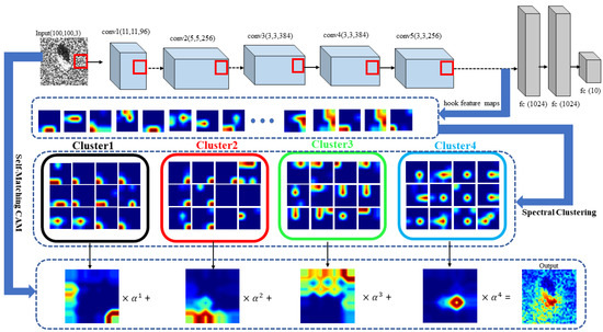
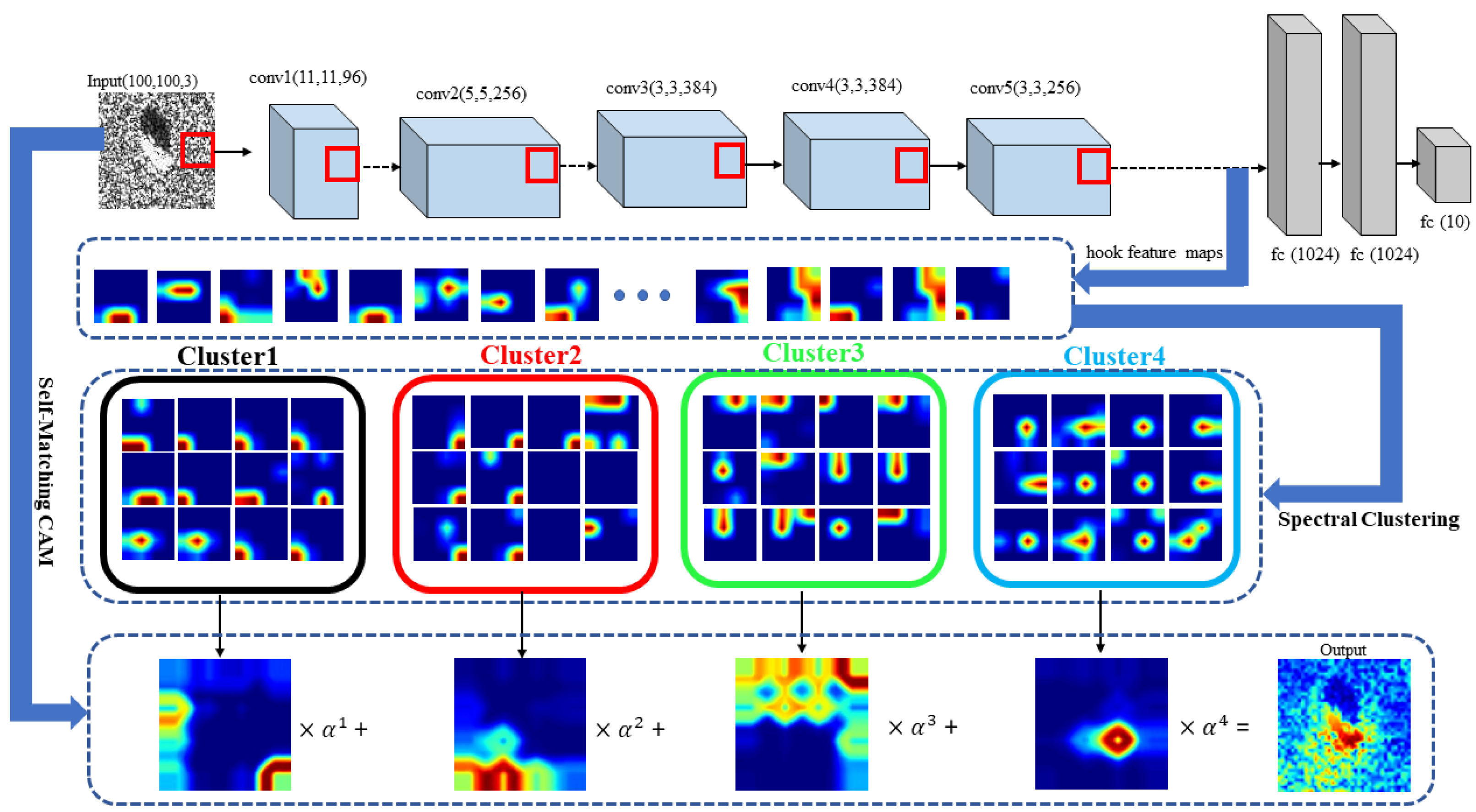
where the weight ${\alpha }_n^c$ is obtained by any of the aforementioned CAM methods. The flowchart of SC-SM CAM is shown in Figure 1. The pseudo-code is presented in Algorithm 1.

Algorithm 1: SC-SM CAM

Input: SAR image ${\mathbf{I}}_N$, model $\mathcal{F}(·)$, spectral clustering $\mathcal{SC}(·)$

$\mathbf{output}$:${\mathbf{H}}_c^{SC-SM}$

initialization:

$\hspace{1em}\hspace{1em}\hspace{1em}{\mathbf{H}}_c^{SC-SM}\leftarrow 0$

$\hspace{1em}\hspace{1em}\hspace{1em}{\mathbf{A}}_M^k\leftarrow$ $\mathcal{F}$(${\mathbf{I}}_N$), k-th feature map

$\mathbf{for}$ n in [1,…,m] $\mathbf{do}$

${\mathbf{A}}^{C_n}={\sum }_n\mathcal{SC}{\left(A_M^k\right)}_n$

${\widehat{\mathbf{A}}}_Q^{C_n}=D{\left({\mathbf{I}}_N\right)}_Q\circ U{\left({\mathbf{A}}^{C_n}\right)}_Q$

# obtain the weights:

${\alpha }_n^c$ ← ${\mathbf{A}}^{C_n}$, $\mathcal{F}$(${\mathbf{I}}_N$)

# generate final heatmap:

${\mathbf{H}}_c^{SC-SM}+={\alpha }_n^{c}Up{\left({\widehat{\mathbf{A}}}_Q^{C_n}\right)}_N$

Figure 1. Flowchart of SC-SM CAM. Here, the AlexNet model is taken as an example.

4. Experimental Results

In this section, the superiority of SC-SM CAM in both validity and efficiency will be demonstrated by numerous experiments. We first perform all the aforementioned CAM methods to compare their class discriminative visualization in Section 4.2. Then, we apply an insertion task to investigate the concentration of highlighted pixels in saliency heatmaps in Section 4.3. Next, two ablation study on two variable parameters will be analyzed in Section 4.4. Finally, we compare the running time of SC-SM CAM with that of the Self-Matching CAM and G-SM CAM to evaluate its computing efficiency in Section 4.5.

4.1. Experiment Setup

All experiments in this paper are conducted on the benchmark dataset MSTAR. MSTAR contains 5172 SAR images corresponding to 10 classes of military vehicles, 2536 for training, and 2636 for validation. All SAR images are size of $1\times 100\times 100$, and normalized to the range $[0,1]$. AlexNet is adopted as a CNN classifier in our experiments (optimizer is stochastic gradient descent (SGD), learning rate = $5\times {10}^{-4}$, and momentum = $0.9$).

4.2. Class Discriminative Visualization

In this section, we first present a qualitative comparison of saliency heatmaps generated by the aforementioned CAM methods, including Grad-CAM, Grad-CAM++, XGrad-CAM, Ablation-CAM, Score-CAM, Self-Matching CAM, G-SM-CAM, and SC-SM CAM, as shown in Figure 2.

Figure 2. Comparison of various CAM methods for MTSTAR SAR images. The ten rows denote vehicles of different classes: 2S1, BRDM_2, BTR_60, D7, SN_132, SN_9563, SN_C71, T62, ZIL131, and ZSU_23_4. The ten columns denote original SAR image, Grad-CAM, Grad-CAM++, XGrad-CAM, Ablation-CAM, Score-CAM, Group-CAM, Self-Matching CAM, G-SM-CAM and SC-SM CAM.

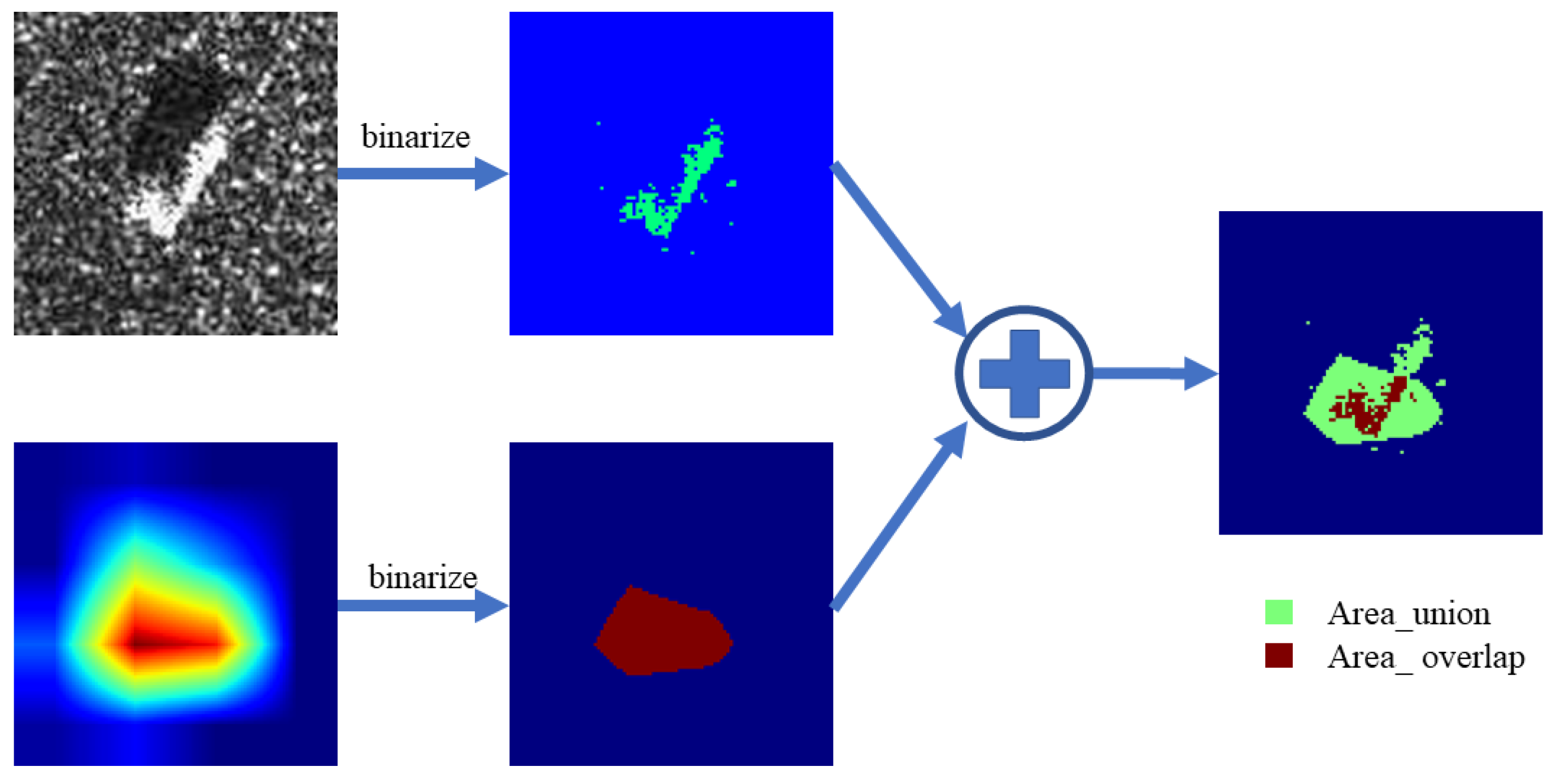
Intuitively, Self-Matching CAM, G-SM-CAM, and SC-SM CAM resemble the original target much more than other optical-based CAM methods. To further demonstrate this, we adopt intersection over union (IoU) to measure the similarity between the original SAR images and their corresponding heatmaps. The definition of IoU in our experiment is:

$$\begin{array}{c}\hfill \mathrm{IoU}=\frac{Area\_overlap}{Area\_union}\end{array}$$

(12)

where $Area\_overlap$ denotes the overlapped area of the highlighted region in the heatmap and its corresponding target area in SAR image, $Area\_union$ denotes the union of both parts, as shown in Figure 3.

Figure 3. Explanation of Area_overlap and Area_union in IoU.

From Equation (12), a high value of IoU means a high similarity between the original images and CAM heatmaps. Note that the ground truth of each image is manually labeled at pixel-level. In Table 1, we compute the IoU of each image in Figure 2.

Table 1. IoU for the SAR images and heatmaps. Each row corresponds to an original SAR image from the first to the tenth row in Figure 2.

Grad	Grad++	XGrad	Ablation	Score	Group	SM	G-SM	SC-SM
$0.187$	$0.204$	$0.177$	$0.235$	$0.279$	$0.210$	$0.504$	$0.588$	$\mathbf{0.659}$
$0.076$	$0.065$	$0.049$	$0.024$	$0.045$	$0.193$	$0.311$	$0.520$	$\mathbf{0.564}$
$0.208$	$0.181$	$0.198$	$0.204$	$0.210$	$0.033$	$0.459$	$0.551$	$\mathbf{0.556}$
$0.229$	$0.090$	$0.137$	$0.130$	$0.110$	$0.362$	$0.590$	$0.663$	$\mathbf{0.729}$
$0.169$	$0.188$	$0.171$	$0.205$	$0.054$	$0.173$	$0.517$	$0.600$	$\mathbf{0.619}$
$0.171$	$0.175$	$0.099$	$0.094$	$0.095$	$0.093$	$0.313$	$0.384$	$\mathbf{0.577}$
$0.162$	$0.117$	$0.135$	$0.133$	$0.152$	$0.126$	$0.408$	$0.634$	$\mathbf{0.638}$
$0.093$	$0.099$	$0.147$	$0.132$	$0.193$	$0.090$	$0.507$	$0.477$	$\mathbf{0.645}$
$0.003$	$0.004$	$0.003$	$0.003$	$0.037$	$0.272$	$0.545$	$0.650$	$\mathbf{0.659}$
$0.254$	$0.131$	$0.178$	$0.205$	$0.010$	$0.243$	$0.533$	$0.658$	$\mathbf{0.670}$

To quantitatively measure the performances of various CAM, Ref. [29] utilizes the “occlusion test” and “conservation test” to demonstrate the superiority of the Self-Matching CAM. In the “occlusion test”, the pixels most relevant to the target are occluded by pixel-multiplying the original SAR image and the binarized heatmap whose high-value elements are set to 0 with a threshold, while the “conservation test” preserve the pixels most relevant to the target. Then, the occluded or conserved images are sent to the CNN to detect the confidence_drop:

$$\begin{array}{c}\hfill confidence\_drop(I,\check{I})=\frac{S_c\left(I\right)-S_c\left(\check{I}\right)}{S_c\left(I\right)}\end{array}$$

(13)

where I refers to the original image and $\check{I}$ refers to the occluded or conserved image. According to the definition of confidence_drop, a high value of confidence_drop in the occlusion test and a low value in the conservation test means that the most discriminative information is contained in the occluded or conserved image. Ref. [29] denotes that only the Self-Matching CAM can simultaneously achieve a high confidence drop in the occlusion and conservation test. A more detailed analysis can be found in [29]. It is clear from the qualitative and quantitative evaluation that only three SAR-based CAM methods can precisely locate the target with a highlighted region in saliency heatmaps, while other, optical-based CAM methods show excessive highlighted regions, which overcover the target. Such overwhelming superiority is benefited from self-matching operations and matches the conclusion in Ref. [29]. Therefore, we will only discuss Self-Matching CAM, G-SM-CAM, and SC-SM CAM.

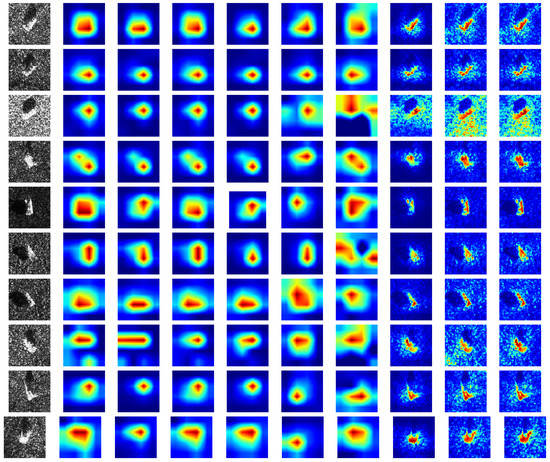
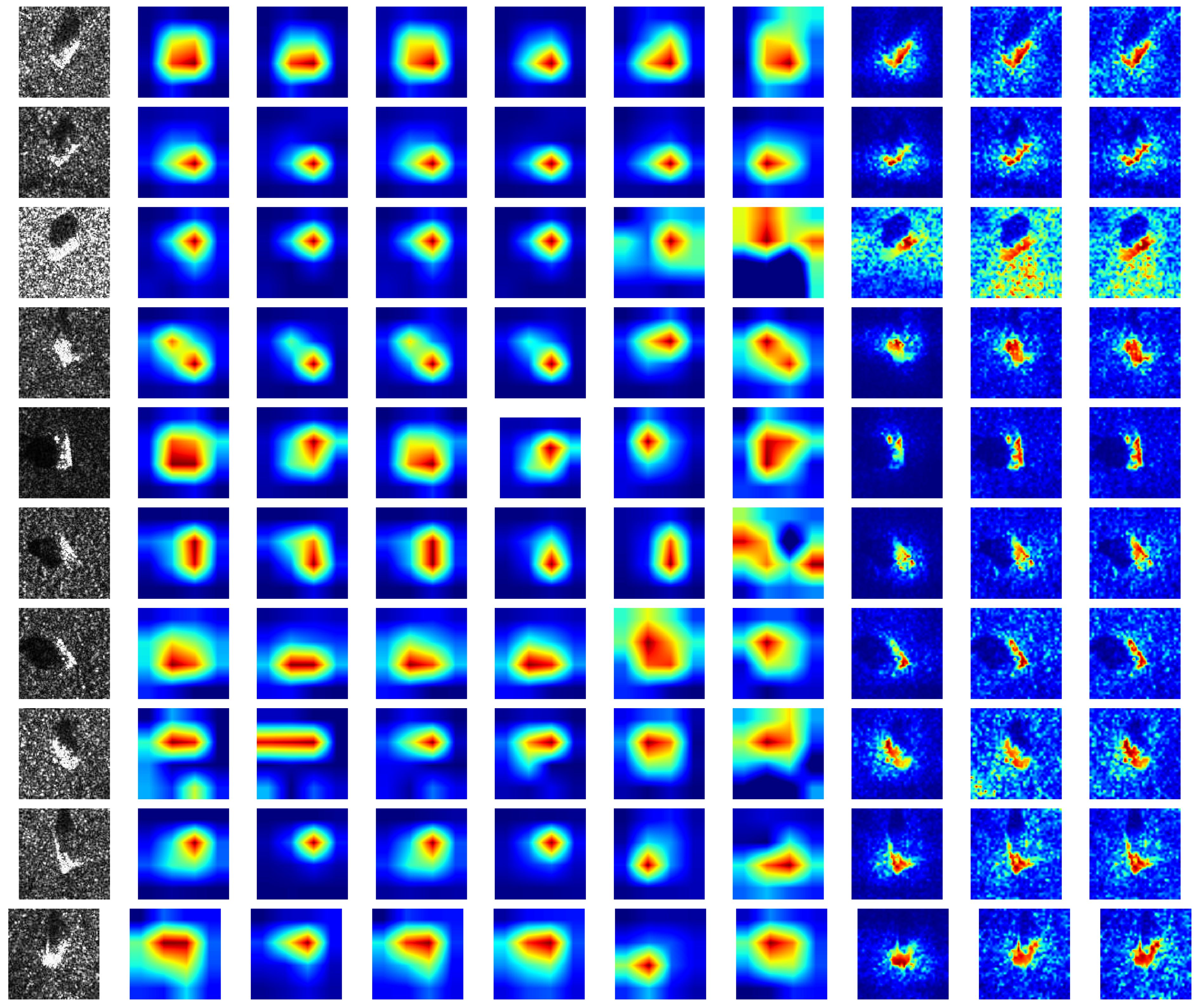
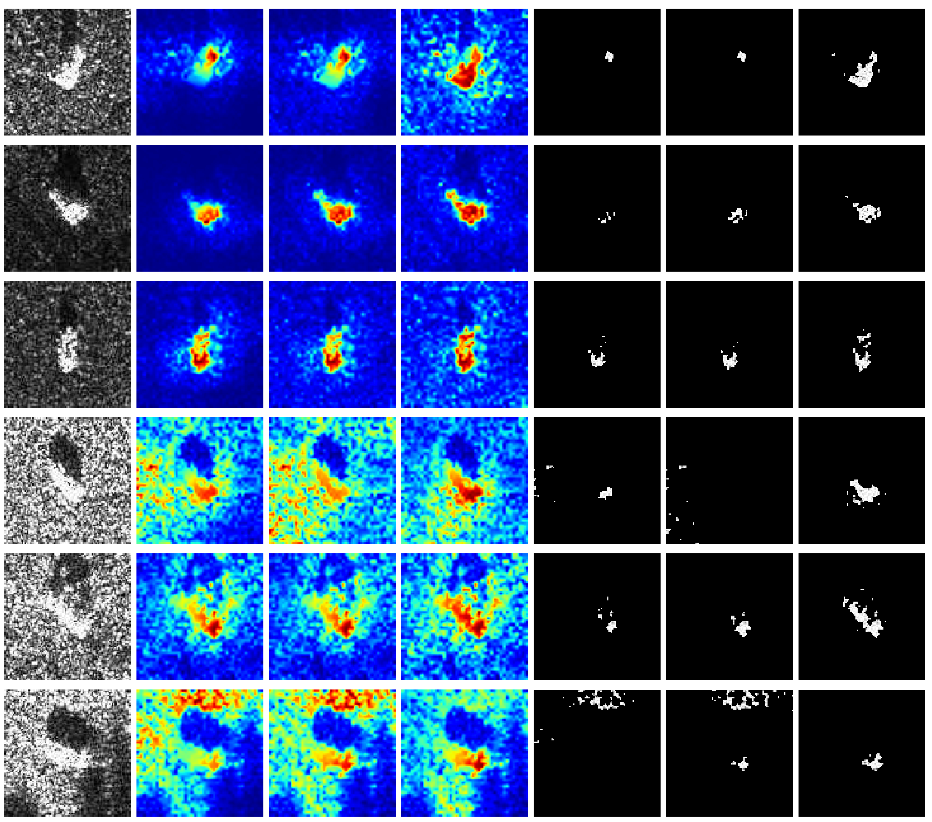
Figure 2 shows some representative SAR images and the saliency heatmaps generated by the three methods. For the images with less noise (e.g., from the first to third rows in Figure 2), although SC-SM CAM may produce more speckles in the background, the most highlighted region matches the target more precisely than Self-Matching CAM and G-SM-CAM. For the images with heavy noise (e.g., from the fourth to sixth rows in Figure 2), all three CAM methods produce numerous speckles, whereas only SC-SM CAM can concentrate the highlighted pixels in the target area. Self-Matching CAM and G-SM CAM even highlight a “wrong” region, irrelevant to the target, for the sixth image in Figure 2. To show this comparison more vividly, we preserve a set of elements in the original SAR images according to the top $20\%$ values in the corresponding saliency heatmaps, as shown in Figure 4 (from the fifth to seventh columns).

Figure 4. Saliency heatmaps of Self-Matching CAM, G-SM CAM, and SC-SM CAM. The first column shows original SAR images. The second to the fourth columns show saliency heatmaps generated by Self-Matching CAM, G-SM CAM, and SC-SM CAM. The fifth to the seventh columns show corresponding masked images.

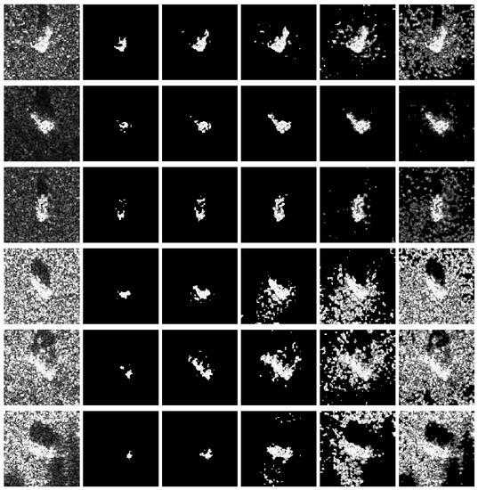
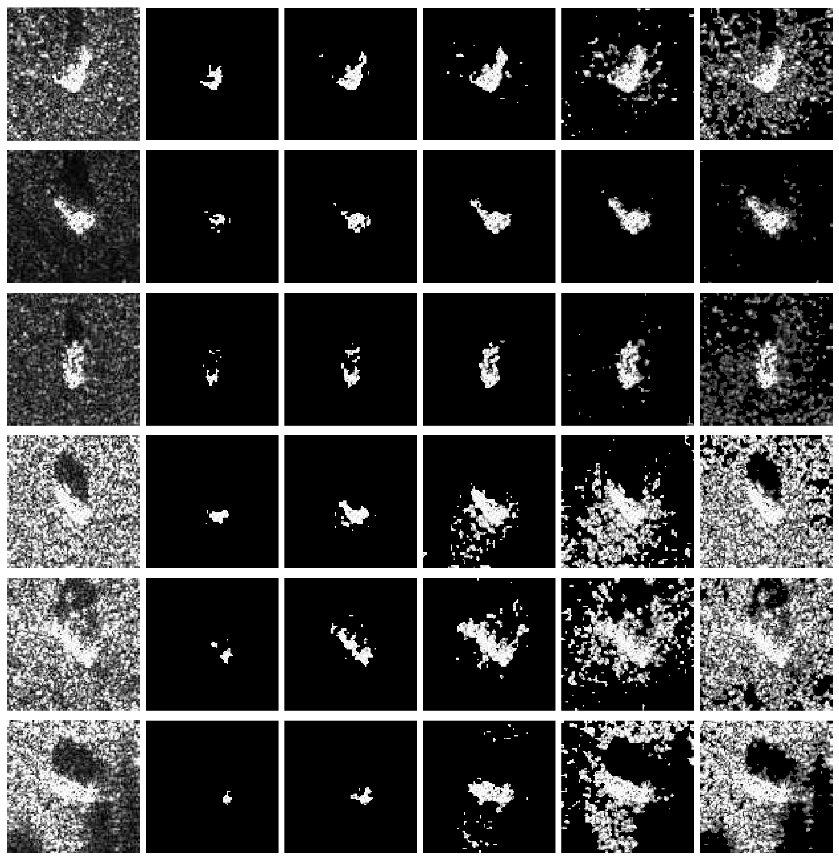
4.3. Insertion Check

We implement an insertion check in this section. Here, the insertion check starts with an all-zero image and gradually recovers contents according to the corresponding saliency heatmaps. Specifically, we replace $1\%$ pixels of the all-zero image until the image is recovered. Figure 5 shows the recovered images of SC-SM CAM with different insertion percentages $\theta$. From Figure 5, we can see that, with only a small $\theta$ ($\theta \le 20\%$), the shape of the target can be recovered. This further demonstrates that pixels with the highest values in saliency heatmaps are accurately concentrated on the target region.

Figure 5. Insertion results generated by SC-SM CAM with different $\theta$. The first column is the original SAR image. The second to the sixth columns are the inserted image when $\theta =10\%,20\%,40\%,60\%,80\%$.

To quantitatively evaluate these methods, we calculate the Area Under Curve (AUC) of the classification score after Softmax with different $\theta$ [34,35].

AUC denotes the area under receiver operating characteristic curve (ROC). For a binary classification problem, ROC refers to the curve of each point, drawn by taking the False Positive (FR) rate as an abscissa and True Positive (TR) rate as an ordinate. AUC can reflect a model’s performance, i.e., AUC = 1, the model’s performance is the best; AUC = 0.5, the model is a random classifier; AUC < 0.5, the model is usually worse than a random classifier. This concept can be extended to multiclass classification problems by regarding the real label as true and other labels as false.

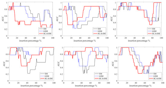
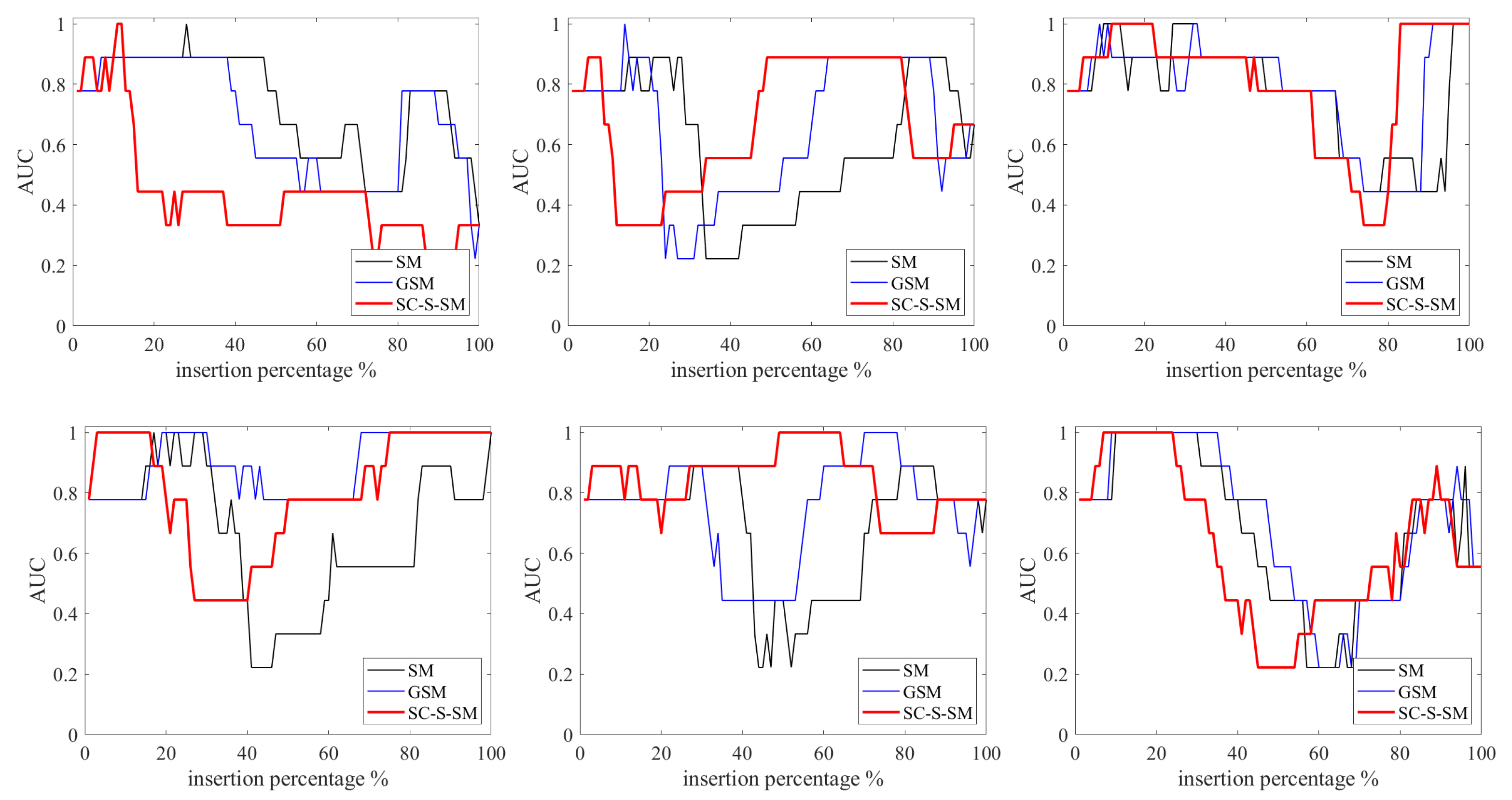
Firstly, we calculate the AUC of the six representative images in Figure 5. The results are shown in Figure 6. The AUC generally increases with $\theta$, sharply drops with a smaller $\theta$, and surges with a larger $\theta$. This is probably because when $\theta$ is small, the re-introduced pixels are concentrated on the target region, which represents the most discriminative feature of the target; whereas, when $\theta$ becomes larger, some sharp or “strange” edges are introduced, resulting in a low AUC. Hence, the earlier arrival of maximal AUC means the most highlighted pixels in the heatmaps are concentrated in the target.

Figure 6. AUC of six representative SAR images, which are calculated by SC-SM CAM with different $\theta$.

Without loss of generality, all 2636 validation images are sent to CNN and the average AUC is calculated from $\theta =5\%$ to $\theta =80\%$, as shown in Table 2. The highest AUC of SC-SM CAM appears when $\theta =15\%$, while this appears when $\theta =30\%$ for the Self-Matching CAM and G-SM CAM. This result further quantitatively validates the perfect precision of SC-SM CAM.

Table 2. Average AUC of each CAM method for all testing data with different $\theta$.

Method	Self-Matching	G-SM CAM	SC-SM CAM
$\theta$ = 5%	0.033	0.057	0.593
$\theta$ = 10%	0.127	0.125	0.667
$\theta$ = 15%	0.379	0.516	$\mathbf{0.906}$
$\theta$ = 20%	0.415	0.579	0.815
$\theta$ = 30%	$\mathbf{0.803}$	$\mathbf{0.825}$	0.815
$\theta$ = 40%	0.516	0.629	0.593
$\theta$ = 50%	0.417	0.530	0.412
$\theta$ = 60%	0.379	0.406	0.267
$\theta$ = 70%	0.415	0.493	0.680
$\theta$ = 80%	0.595	0.639	0.886

4.4. Ablation Study

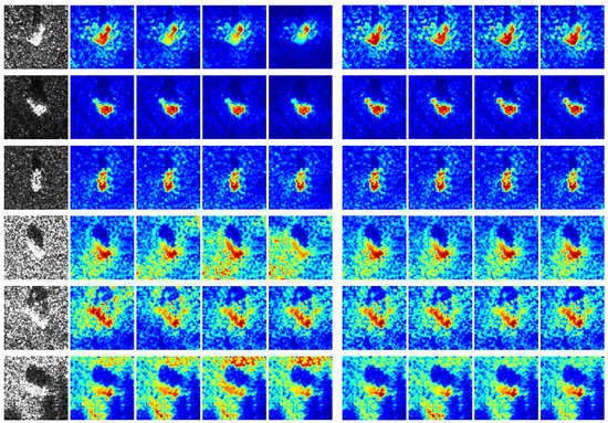
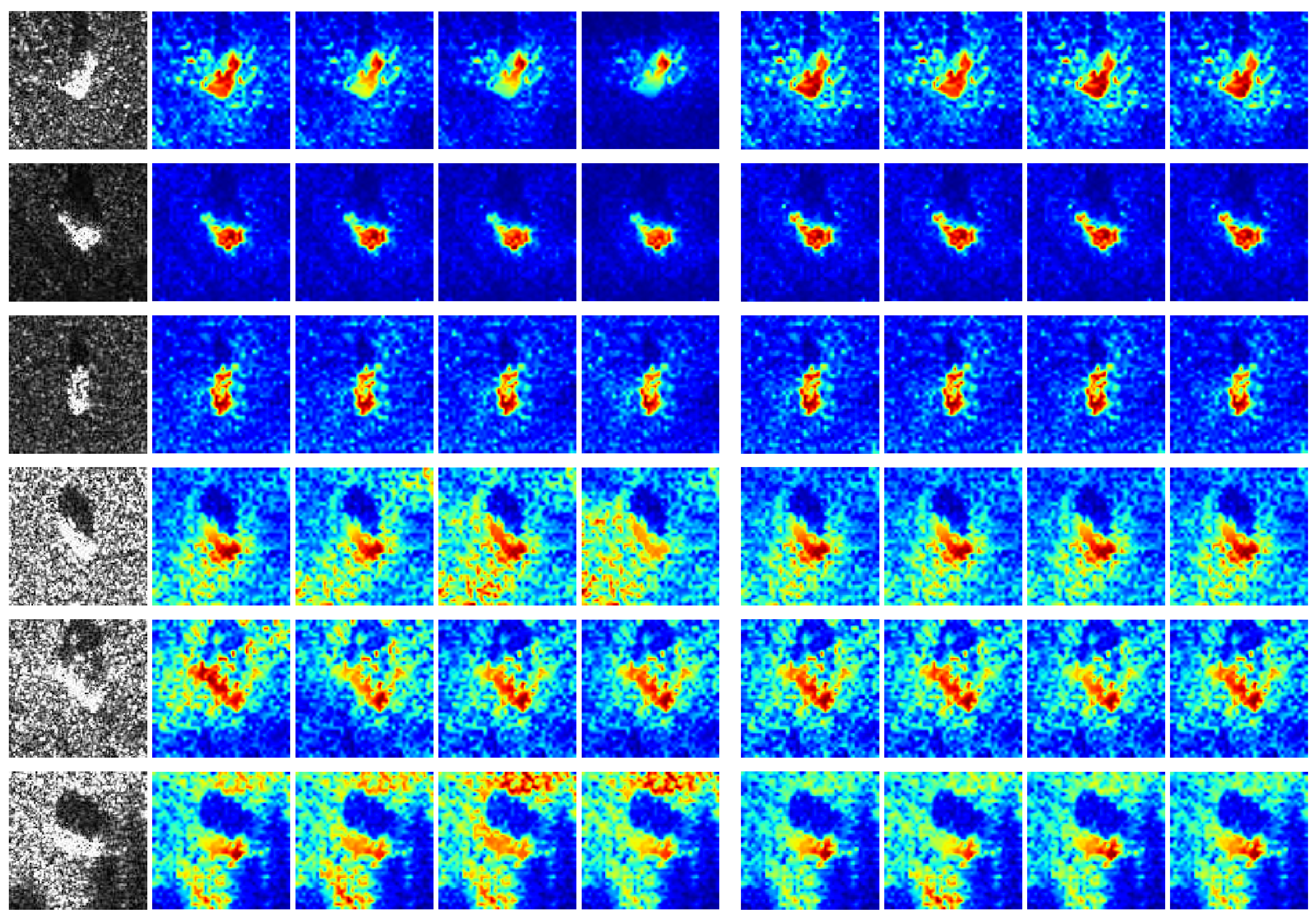
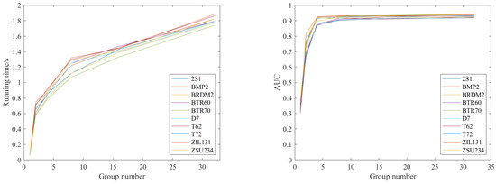
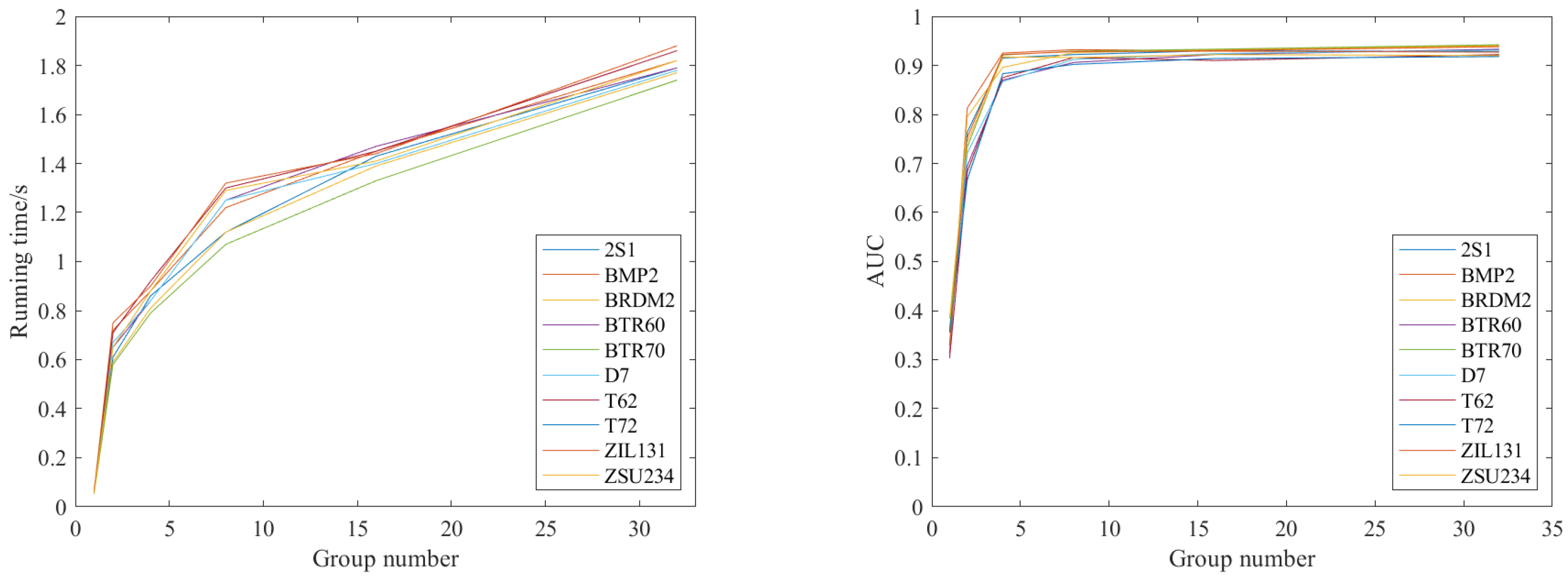
Both G-SM-CAM and SC-SM CAM adopt the “grouping” strategy; thus, we investigated the influence of group number G on the saliency heatmaps generated by G-SM CAM and SC-SM CAM, respectively. The results are shown in Figure 7. Apparently, the number of speckles in the saliency heatmaps of G-SM CAM decreases when G rises, while the saliency heatmaps of SC-SM CAM are nearly unrelated to G. This is because the groups in G-SM CAM are categorized according to channel indices. In this case, different G may divide feature maps with huge divergence into one group. In comparison, spectral clustering can ensure that similar feature maps are divided into a group in SC-SM CAM. According to our experimental results, we find that similar feature maps can be categorized into several groups, whereas the all-zero feature maps are distributed in the rest of the groups when G changes. Here, we further investigate the optimal G for 10 classes of SAR images. We record the running time and AUC when the top $15\%$ highlighted pixels are conserved. ($\theta =15\%$ in insertion check) with $G=1,2,4,8,16,32$, respectively, as shown in Figure 8. In general, the running time increases with G for each class. It is clear from the left subfigure in Figure 8 that the running time of SC-SM CAM is shorter than the median when $G\le 4$. Note that the running time of $G=1$ is much shorter than other G. This is because SC-SM CAM degrades into G-SM-CAM when $G=1$ (spectral clustering is not required). As for AUC, it is clear from the right subfigure in Figure 8 that the AUC is very low when $G=1$ and $G=2$, whereas it improves dramatically when $G=4$ and then almost retains this high value when $G>4$. This is because these similar feature maps can be divided into a group when G is small. In contrast, when $G>4$, the feature maps with high similarity can be divided into a group; thus, the AUC is almost unchanged. This result intuitively matches the heatmaps with different G in Figure 7.

Figure 7. Saliency heatmaps generated by G-SM-CAM and SC-SM CAM with different G. The first columns are original SAR images. The second to the fifth columns are generated by G-SM-CAM when $G=4$, 8, 16, 32. The sixth to the ninth columns are generated by SC-SM CAM when $G=4$, 8, 16, 32.

Figure 8. Running time and AUC for 10 classes of vehicles with different G. The left figure is running time with $G=1,2,4,8,16,32$. The right figure is AUC when the top $15\%$ highlighted pixels are conserved. ($\theta =15\%$ in insertion check) with $G=1,2,4,8,16,32$.

Based on the above analysis, we think $G=4$ is the optimal group number for MSTAR dataset which is a balance between effect and efficiency. Therefore, our experiments are all conducted with $G=4$ unless otherwise specified. Besides, it should be pointed out that $G=4$ is only optimal for MSTAR dataset, whereas, the optimal G probably changes for other SAR image datasets. This ablation experiment further demonstrates that spectral clustering works effectively in grouping feature maps.

4.5. Computing Efficiency

In this section, we will investigate the computational efficiency of our proposed method. We record the average running time of 2636 validation SAR images of Self-Matching CAM, G-SM CAM, and SC-SM CAM on 8th Gen Intel Core(TM) i7-8700, $3.20$ GHz, as shown in Table 3. It is clear from Table 3 that SC-SM CAM runs approximately twice as fast as Self-Matching CAM. It should be noted that, although G-SM-CAM runs much faster than the other methods, this high speed comes at the cost of visualization effects, whereas SC-SM CAM improves both the effect and the efficiency.

Table 3. Average running time of each CAM method.

Method	Running Time/s
Self-Matching CAM	$0.863$
G-SM-CAM (G = 4)	$\mathbf{0.068}$
SC-SM CAM (G = 4)	$0.449$

In addition, we further study the effect of the number of the eigenvectors on running time, as shown in Table 4. From Table 4, the number of the eigenvectors has no conspicuous influence on running time.

Table 4. Average running time with different numbers of eigenvectors.

Number of Eigenvectors	Running Time/s
4	$0.424$
10	$0.440$
50	$0.439$
100	$0.440$
256	$0.449$

5. Discussion

In our experiment, the effect and efficiency of SC-SM CAM are verified through both qualitative (class discriminative visualization and ablation study) and quantitative (insertion check and running time) analysis. Class discriminative visualization provides a vivid comparison of various CAM methods, especially the divergence among the three self-matching-based methods. An ablation study shows that an appropriate number of eigenvectors in the Laplacian matrix have a significant impact on the visualization effect of SC-SM CAM, whereas the number of clusters has a nominal influence. AN insertion check further demonstrates the SC-SM CAM concentrates the more high-value pixels in the target area in comparison to G-SM-CAM and Self-Matching CAM. The running time demonstrates the superiority of SC-SM CAM in terms of computational efficiency.

It should be noted that it is possible to strike a balance between the number of eigenvectors and the visualization effect. Seeking an optimal number of eigenvectors is our further research direction.

6. Conclusions

In this paper, we propose SC-SM CAM, an efficient visual interpretation algorithm of CNN, for target recognition of SAR images. In visualization effects, two SOTA SAR-based CAM methods, Self-Matching CAM and G-SM-CAM, SC-SM CAM, can highlight the target area in saliency heatmaps more precisely than G-SM-CAM and Self-Matching CAM. In comparison to G-SM-CAM, the fastest of these three methods at the cost of effect, SC-SM CAM increases speed without any loss of visualization effect. Numerous experimental results verify the validity of SC-SM CAM through quantitative and qualitative analyses. These findings may shed light on the understanding of the inner mechanism of CNN classification.

References

- Pallotta, L.; Clemente, C.; Maio, A.D.; Soraghan, J.J. Detecting Covariance Symmetries in Polarimetric SAR Images. IEEE Trans. Geosci. Remote Sens. 2017, 55, 80–95. [Google Scholar] [CrossRef]
- Wang, Z.; Wang, S.; Xu, C.; Li, C.; Yue, B.; Liang, X. SAR Images Super-resolution via Cartoon-texture Image Decomposition and Jointly Optimized Regressors. In Proceedings of the 2017 International Geoscience and Remote Sensing Symposium, Fort Worth, TX, USA, 23–28 July 2017; pp. 1668–1671. [Google Scholar]
- Li, W.; Zou, B.; Zhang, L. Ship Detection in a Large Scene SAR Image Using Image Uniformity Description Factor. In Proceedings of the 2017 SAR in Big Data Era: Models, Methods and Applications, Beijing, China, 13–14 November 2017; pp. 1–5. [Google Scholar]
- Yuan, Y.; Wu, Y.; Fu, Y.; Wu, Y.; Zhang, L.; Jiang, Y. An Advanced SAR Image Despeckling Method by Bernoulli-Sampling-Based Self-Supervised Deep Learning. Remote Sens. 2021, 13, 3636. [Google Scholar] [CrossRef] [Scilit]
- Wang, Y.; Zhang, Y.; Qu, H.; Tian, Q. Target Detection and Recognition Based on Convolutional Neural Network for SAR Image. In Proceedings of the 2018 11th International Congress on Image and Signal Processing, Biomedical Engineering and Informatics, Beijing, China, 13–15 October 2018; pp. 1–5. [Google Scholar]
- Ding, B.; Wen, G.; Huang, X.; Ma, C.; Yang, X. Data Augmentation by Multilevel Reconstruction Using Attributed Scattering Center for SAR Target Recognition. IEEE Geosci. Remote Sens. Lett. 2017, 14, 979–983. [Google Scholar] [CrossRef] [Scilit]
- Xiong, K.; Zhao, G.; Wang, Y.; Shi, G. SPB-Net: A Deep Network for SAR Imaging and Despeckling with Downsampled Data. IEEE Trans. Geosci. Remote Sens. 2020. [Google Scholar] [CrossRef] [Scilit]
- Luo, Y.; An, D.; Wang, W.; Huang, X. Improved ROEWA SAR Image Edge Detector Based on Curvilinear Structures Extraction. IEEE Geosci. Remote Sens. Lett. 2020, 17, 631–635. [Google Scholar] [CrossRef] [Scilit]
- Zhang, L.; Liu, Y. Remote Sensing Image Generation Based on Attention Mechanism and VAE-MSGAN for ROI Extraction. IEEE Geosci. Remote Sens. Lett. 2021. [Google Scholar] [CrossRef] [Scilit]
- Min, R.; Lan, H.; Cao, Z.J.; Cui, Z.Y. A Gradually Distilled CNN for SAR Target Recognition. IEEE Access 2019, 7, 42190–42200. [Google Scholar] [CrossRef] [Scilit]
- Zhou, F.; Wang, L.; Bai, X.R.; Hui, Y.; Zhou, Z. SAR ATR of Ground Vehicles Based on LM-BN-CNN. IEEE Trans. Geosci. Remote Sens. 2018, 56, 7282–7293. [Google Scholar] [CrossRef] [Scilit]
- Yu, J.; Zhou, G.; Zhou, S. A Lightweight Fully Convolutional Neural Network for SAR Automatic Target Recognition. Remote Sens. 2021, 13, 3029. [Google Scholar] [CrossRef] [Scilit]
- Dong, Y.P.; Su, H.; Wu, B.Y. Efficient Decision-based Black-box Adversarial Attacks on Face Recognition. In Proceedings of the 2019 IEEE/CVF Conference on Computer Vision and Pattern Recognition (CVPR), Long Beach, CA, USA, 15–20 June 2019. [Google Scholar]
- Mopuri, K.R.; Garg, U.; Babu, R.V. CNN Fixations: An Unraveling Approach to Visualize the Discriminative Image Regions. IEEE Trans Image Process. 2017, 28, 2116–2125. [Google Scholar] [CrossRef] [Scilit] [PubMed]
- Montavon, G.; Binder, A.; Lapuschkin, S.; Samek, W.; Müller, K.R. Layer-Wise Relevance Propagation: An Overview. In Explainable AI: Interpreting, Explaining and Visualizing Deep Learning; Samek, W., Montavon, G., Vedaldi, A., Hansen, L., Müller, K.R., Eds.; Springer: Cham, Switzerland, 2019; pp. 14–15. [Google Scholar]
- Giacalone, J.; Bourgeois, L.; Ancora, A. Challenges in aggregation of heterogeneous sensors for Autonomous Driving Systems. In Proceedings of the 2019 IEEE Sensors Applications Symposium, Sophia Antipolis, France, 11–13 March 2019; pp. 1–5. [Google Scholar]
- Zhu, C.; Chen, Z.; Zhao, R.; Wang, J.; Yan, R. Decoupled Feature-Temporal CNN: Explaining Deep Learning-Based Machine Health Monitoring. IEEE Trans. Instrum. Meas. 2021, 70, 1–13. [Google Scholar] [CrossRef] [Scilit]
- Petsiuk, V.; Das, A.; Saenko, K. RISE: Randomized input sampling for explanation of black-box models. In Proceedings of the British Machine Vision Conference 2018, Newcastle, UK, 3–6 September 2018. [Google Scholar]
- Amin, M.G.; Erol, B. Understanding deep neural networks performance for radar-based human motion recognition. In Proceedings of the 2018 IEEE Radar Conference, Oklahoma City, OK, USA, 23–27 April 2018; pp. 1461–1465. [Google Scholar]
- Kapishnikov, A.; Bolukbasi, T.; Viégas, F.; Terry, M. Viégas, and Michael Terry. XRAI: Better attributions through regions. In Proceedings of 2019 IEEE/CVF International Conference on Computer Vision, ICCV 2019, Seoul, Korea, 27 October–2 November 2019; pp. 4947–4956. [Google Scholar]
- Bach, S.; Binder, A.; Montavon, G.; Klauschen, F.; Müller, K.R. On Pixel-Wise Explanations for Non-Linear Classifier Decisions by Layer-Wise Relevance Propagation. PLoS ONE 2015, 10, e0130140. [Google Scholar] [CrossRef] [Scilit] [PubMed]
- Zhou, B.; Khosla, K.; Lapedriza, A.; Oliva, A.; Torralba, A. Learning Deep Features for Discriminative Localization. In Proceedings of the 2016 IEEE/CVF Conference on Computer Vision and Pattern Recognition (CVPR), Las Vegas, NV, USA, 26 June–1 July 2016. [Google Scholar]
- Ramprasaath, R.S.; Michael, C.; Abhishek, D. Grad-CAM: Visual Explanations from Deep Networks via Gradient-based Localization. arXiv 2015, arXiv:1610.02391v4. [Google Scholar]
- Aditya, C.; Anirban, S.; Abhishek, D.; Prantik, H. Grad-CAM++: Improved Visual Explanations for Deep Convolutional Networks. arXiv 2018, arXiv:1710.11063v34. [Google Scholar]
- Fu, H.G.; Hu, Q.Y.; Dong, X.H.; Guo, Y.I.; Gao, Y.H.; Li, B. Axiom-based Grad-CAM: Towards Accurate Visualization and Explanation of CNNs. In Proceedings of the 2020 31th British Machine Vision Conference (BMVC), Manchester, UK, 7–10 September 2020. [Google Scholar]
- Saurabh, D.; Harish, G.R. Ablation-CAM: Visual Explanations for Deep Convolutional Network via Gradient-free Localization. In Proceedings of the 2020 IEEE Winter Conference on Applications of Computer Vision (WACV), Snowmass, CO, USA, 1–5 March 2020. [Google Scholar]
- Wang, H.F.; Wang, Z.F.; Du, M.N. Methods for Interpreting and Understanding Deep Neural Networks. In Proceedings of the 2020 IEEE/CVF Conference on Computer Vision and Pattern Recognition Workshops (CVPRW), Seattle, WA, USA, 14–19 June 2020. [Google Scholar]
- Feng, Z.; Zhu, M.; Stanković, L.; Ji, H. Self-Matching CAM: A Novel Accurate Visual Explanation of CNNs for SAR Image Interpretation. Remote Sens. 2021, 13, 1772. [Google Scholar] [CrossRef] [Scilit]
- Zhang, Q.; Rao, L.; Yang, Y. Group-CAM: Group Score-Weighted Visual Explanations for Deep Convolutional Networks. arXiv 2021, arXiv:2103.13859. [Google Scholar]
- Huang, D.; Wang, C.; Wu, J.; Lai, J.; Kwoh, C. Ultra-Scalable Spectral Clustering and Ensemble Clustering. IEEE Trans. Knowl. Data Eng. 2020, 32, 1212–1226. [Google Scholar] [CrossRef] [Scilit]
- Wei, Y.; Niu, C.; Wang, H.; Liu, D. The Hyperspectral Image Clustering Based on Spatial Information and Spectral Clustering. In Proceedings of the 2019 IEEE 4th International Conference on Signal and Image Processing (ICSIP), Wuxi, China, 19–21 July 2019; pp. 127–131. [Google Scholar]
- Zhu, W.; Nie, F.; Li, X. Fast Spectral Clustering with Efficient Large Graph Construction. In Proceedings of the 2017 IEEE International Conference on Acoustics, Speech and Signal Processing (ICASSP), New Orleans, LA, USA, 5–9 March 2017; pp. 2492–2496. [Google Scholar]
- Stanković, L.J.; Mandic, D.; Daković, M.; Brajović, M.; Scalzo-Dees, B.; Li, S.; Constantinides, A.G. Data Analytics on Graphs—Part III: Machine Learning on Graphs, from Graph Topology to Applications. Found. Trends Mach. Learn. 2020, 13, 332–530. [Google Scholar] [CrossRef] [Scilit]
- Huo, J.; Gao, Y.; Shi, Y.; Yin, H. Cross-Modal Metric Learning for AUC Optimization. IEEE Trans. Netw. Learn. 2017, 29, 4844–4856. [Google Scholar] [CrossRef] [Scilit] [PubMed]
- Gultekin, S.; Saha, A.; Ratnaparkhi, A.; Paisley, J. MBA: Mini-Batch AUC Optimization. IEEE Trans. Netw. Learn. 2020, 31, 5561–5574. [Google Scholar] [CrossRef] [Scilit] [PubMed]
Publisher’s Note: MDPI stays neutral with regard to jurisdictional claims in published maps and institutional affiliations. |
© 2021 by the authors. Licensee MDPI, Basel, Switzerland. This article is an open access article distributed under the terms and conditions of the Creative Commons Attribution (CC BY) license (https://creativecommons.org/licenses/by/4.0/).