Article

An Optimized Deep Neural Network for Overhead Contact System Recognition from LiDAR Point Clouds

1
College of Computer Science and Electronic Engineering, Hunan University, Changsha 410082, China
2
Department of Image and Network Investigation, Railway Police College, Zhengzhou 450053, China
*
Author to whom correspondence should be addressed.
Remote Sens. 2021, 13(20), 4110; https://doi.org/10.3390/rs13204110
Submission received: 19 August 2021 / Revised: 6 October 2021 / Accepted: 8 October 2021 / Published: 14 October 2021

Abstract

:
As vital infrastructures, high-speed railways support the development of transportation. To maintain the punctuality and safety of railway systems, researchers have employed manual and computer vision methods to monitor overhead contact systems (OCSs), but they have low efficiency. Investigators have also used light detection and ranging (LiDAR) to generate point clouds by emitting laser beams. The point cloud is segmented for automatic OCS recognition, which improves recognition efficiency. However, existing LiDAR point cloud segmentation methods have high computational/model complexity and latency. In addition, they cannot adapt to embedded devices with different architectures. To overcome these issues, this article presents a lightweight neural network EffNet consisting of three modules: ExtractA, AttenA, and AttenB. ExtractA extracts the features from the disordered and irregular point clouds of an OCS. AttenA keeps information flowing in EffNet while extracting useful features. AttenB uses channel and spatialwise statistics to enhance important features and suppress unimportant ones efficiently. To further speed up EffNet and match it with diverse architectures, we optimized it with a generation framework of tensor programs and deployed it on embedded systems with different architectures. Extensive experiments demonstrated that EffNet has at least a 0.57% higher mean accuracy, but with 25.00% and 9.30% lower computational and model complexity for OCS recognition than others, respectively. The optimized EffNet can be adapted to different architectures. Its latency decreased by 51.97%, 56.47%, 63.63%, 82.58%, 85.85%, and 91.97% on the NVIDIA Nano CPU, TX2 CPU, UP Board CPU, Nano GPU, TX2 GPU, and RTX 2,080 Ti GPU, respectively.

1. Introduction

High-speed railways have given rise to significant changes in the way people live and work. For the safe operation of high-speed railways, the overhead catenary system (OCS) must be monitored. The OCS includes an insulator, cantilever, pole, contact wire, catenary wire, registration arm, steady arm, and dropper. The OCS components are susceptible to natural conditions, such as weather and wind, and they may loosen and break due to constant exposure to the outdoors. These problems cause security risks for the operation of high-speed railways. Professional railway workers often manually recognize and measure geometric parameters related to the spatial geometric positions of the catenary in an OCS, such as lead height and pull-out values. The lead height is the vertical height of the contact wire from a rail surface. The pull-out value is the offset between a contact wire and the center of a pantograph skateboard in electrified trains. However, manual detection may cause large errors and slow speed. Therefore, intelligent OCS recognition methods should be developed to increase the accuracy and speed of inspection.
Recently, as a noncontact measuring method, light detection and ranging (LiDAR) emits laser beams and measures the distances from LiDAR to object points in various scenarios. In addition, LiDAR measures the strength of the return. LiDAR is widely applied in diverse fields such as three-dimensional (3D) object recognition [1], cultural heritage representation [2], and OCS recognition [3], due to its high accuracy, reliability, and efficiency. Through LiDAR, OCS components are scanned, and then, their point clouds are generated. Based on point cloud segmentation, the OCS is recognized for railway system inspection. Figure 1 shows that individual components of an OCS can be segmented from LiDAR point clouds. Additionally, LiDAR is not affected by extraneous obstacles such as trees in high-speed railway scenarios, as the obstacles are strictly restricted to places far from an OCS. In sum, LiDAR has several advantages for OCS recognition:
  • High accuracy: The result of LiDAR measurement is more accurate than the result of manual measurement. In addition, the distance measurement of LiDAR is generally more precise than that of computer vision methods [4,5,6,7];
  • High efficiency: The measurement of LiDAR accelerates OCS recognition compared with manual measurement. LiDAR point clouds do not require as much processing time as high-resolution images produced by cameras;
  • High reliability: Irrelevant interferents are easily filtered by LiDAR, such as the SICK LMS511-20100 PRO LiDAR employed in this article. For example, the measurement error of the LMS511-20100 PRO LiDAR reaches the millimeter level. High measurement accuracy enables high reliability for OCS recognition;
  • Low requirements: LiDAR has almost no requirements on the measurement environment, such as lighting conditions, while computer vision methods have strict requirements for light conditions.
Researchers segmented point clouds for OCS recognition by proposing various approaches, such as traditional machine learning and deep learning technologies. However, traditional machine learning methods, such as [8,9], have low efficiency and high complexity, overly relying on prior knowledge and handcrafted features. With the advancement of deep learning [10], many researchers have adopted deep neural networks (DNNs) for OCS recognition. For example, Qi et al. [11,12] developed the PointNet and PointNet++ models to segment point clouds. Chen et al. [13] improved PointNet++ to concentrate global and point-level features of a center point into local features for point cloud recognition. Other methods [4,5,7] relied on images to inspect an OCS with DNNs, but high-resolution images allowed a larger amount of calculation than point clouds. To further improve OCS recognition, the approach in [14] leveraged the k-nearest neighbors algorithm (KNN) [15] and DNNs to process point clouds of an OCS in real high-speed scenarios. As the point density and distribution pattern influence point cloud segmentation, Lin et al. [14] adopted data from a fixed scan area. They summed the previous and next frames and obtained the 3D coordinate values of the current frame. Then, the above impact of density and distribution was alleviated. Although these technologies achieved a certain increase in accuracy, they faced the following challenges when running on embedded platforms:
  • High computational complexity: The above methods usually use complex model structures to improve the accuracy of OCS recognition. The complex algorithm structures increase the computational complexity;
  • High latency: As the above methods have more computational operations, their latency is higher than simple models. They are also rarely accelerated to achieve low inference latency on embedded systems;
  • High model complexity: Due to the intensive computation, the above methods have a high model complexity, which is a burden for embedded devices.
If computational/model complexity and latency are reduced, OCS recognition on embedded devices will become possible. To this end, a lightweight neural network is required. In general, lightweight neural networks refer to a more efficient DNN calculation model. It is constructed by decreasing computational and model complexity while ensuring that the loss of model precision is low. We designed a lightweight neural network, EffNet, which contains three modules: ExtractA, AttenA, and AttenB. The ExtractA module extracts features from the disordered and irregular point clouds of an OCS based on the work [14], where some of the authors also participated in this paper. AttenA refines features relying on the study [16]. AttenB enhances the vital features and fades out unimportant ones based on the method in [17]. AttenA and AttenB are attention mechanisms. Here, the attention mechanism is an approach that imitates human cognitive attention. It concentrates on relevant features and overlooks the unimportant ones in deep learning [18]. The advantages of AttenA and AttenB are different. AttenA focuses on the effectiveness of extracted features. AttenB emphasizes the efficiency of attention mechanisms. AttenB is more lightweight than AttenA, and AttenA extracts more features than AttenB. The three modules are integrated for accurate OCS recognition. The interaction of these modules also improves the efficiency of OCS recognition.
To further decrease the latency of EffNet and adapt it to different architectures, we accelerated it with an Auto-scheduler [19]. When speeding up EffNet, we matched it with different architectures so that it can be applied to embedded devices. For the adaptability study of EffNet on diverse architectures, we selected prevalent devices, such as the NVIDIA RTX 2080 Ti GPU with the Turing architecture, Jetson Nano GPU with the Maxwell architecture, Nano CPU with the ARM architecture, UP Board CPU with the Intel x86 architecture, Jetson TX2 GPU with the Pascal architecture, and TX2 CPU with the ARM architecture. We matched EffNet with the x86 or ARM architectures using the low level virtual machine (LLVM) [20] and adapted EffNet to the Pascal, Turing, or Maxwell architectures using the Compute Unified Device Architecture (CUDA) [21]. To optimize EffNet, we analyzed its computation graphs and divided them into subgraphs for a series of tasks. These tasks were analyzed with the program sampler in the Auto-scheduler for several tensor programs. Then, the performance of the tensor programs was fine-tuned through an evolutionary search [22] and a learnable cost model [23]. We used a remote procedure call (RPC) framework to reduce the tuning time of EffNet. With the iterative tuning process, the high-performance host generates the best performance tensor program and sends it to the embedded devices for fast inference. Our contributions are summarized below:
(1)
We designed a lightweight neural network, EffNet, to segment point clouds for OCS recognition. EffNet was integrated with ExtractA, AttenA, and AttenB. The three modules have different functions and handle different tasks separately; that is, when features need to be extracted, we employed the ExtractA module. We adopted the AttenA module when it was necessary to make information flow in neural networks and extract features, simultaneously. We used the AttenB module when needing to focus on attention mechanism efficiency. Benefiting from these three modules, EffNet increased the mean recognition accuracy of point clouds by 0.57% for OCS recognition with lower model/computational complexity and a higher speed than others;
(2)
We optimized EffNet with a generation framework of tensor programs (Auto-scheduler) to further accelerate it and adapted to different device architectures. The Auto-scheduler can generate corresponding tensor programs for each subgraph, according to defined tasks. Then, the tensor programs were auto-tuned with RPC, which uses the computing power of a high-performance host for fast calculation. The host conducted the reproduction, crossover, and mutation of the configuration parameters relying on a learnable cost and an evolutionary search model. The host generated possibly higher-quality tensor programs. The tensor programs were adapted to different hardware architectures on devices through different technologies such as LLVM and CUDA. Then, with iterative tuning on the host, we could obtain the best-performing tensor program, which had the least latency when running on the embedded devices;
(3)
We performed extensive experiments to validate EffNet on different architectures in complex high-speed railway scenarios. The experiments confirmed that EffNet is effective at recognizing point clouds for OCS recognition. EffNet also matches different architectures. The mean accuracy of EffNet was at least 1.13% higher in the intersection over union (IoU) than that of similar methods. The optimized EffNet had the same accuracy and computational/model complexity as before. Compared with other methods, the optimized EffNet obtained the same accuracy range, but its model and computational complexities were at least 9.30% and 25.00% lower. In addition, the optimized EffNet reduced the inference latency by 91.97%, 51.97%, 82.58%, 56.47%, 63.63%, and 85.85% on the RTX 2,080 Ti GPU, Nano CPU, Nano GPU, TX2 CPU, UP Board CPU, and TX2 GPU, respectively.

2. Related Work

Many intelligent approaches have been proposed for OCS recognition. They can be classified into two groups: ones relying on traditional machine learning studies [8,9,24] and ones based on deep learning technologies [5,7,11,12,14,25]. Specifically, Han et al. [8] divided the cantilevers of an OCS into multiple parts using locally convex connected patches (LCCPs) and super voxel clustering (SVC) algorithms. Then, the features of the parts were extracted. Based on the features, the coordinates of the connection points of the parts were calculated with the augmented random sample consensus (RANSAC) algorithm. Furthermore, the coordinates were employed to detect the status of the connection points. Pastucha et al. [9] also used RANSAC algorithms and geometric rules to recognize the cantilever. Chen et al. [24] adopted spatial regularity and a smoothness constraint for OCS recognition with the multiscale conditional random field (CRF). However, these studies mainly recognized specified parts of an OCS, and they are difficult to extend to new recognition tasks in an OCS. The reason for this is that point cloud features need to be depicted artificially in these traditional approaches, so the choice of features has a strong influence on the recognition precision. Selecting useful features still requires a high cost of design and experiments. The features of manual description restrict the expansion of such methods for new tasks. In summary, the traditional methods are limited by prior knowledge, applicable scenarios, and handcrafted information. Additionally, these algorithms have high latency, which is a challenge for embedded platforms.
Currently, researchers usually adopt deep learning technologies to improve model accuracy [5,7,11,12,14,25]. For example, the method [5] leveraged Faster R-CNN networks [26] and a denoising autoencoder to detect the insulator surface in an OCS based on images. Wei et al. [7] used DNNs to monitor the pantograph in an OCS by processing images. These methods relied on images that were captured by cameras. Cameras are limited by severe weather conditions. When the light is poor, cameras need auxiliary light for clear images. In contrast, LiDAR does not need auxiliary light to generate point clouds. The point cloud can be used for OCS recognition without the influence of weather conditions. For instance, the classic work [11] proposed PointNet for point cloud segmentation. PointNet also enhances the precision of object segmentation and recognition, but it considers no features of local structures in neighborhoods. Thus, relevant features are easily lost, and the effect is poor for large-scale scene recognition. To alleviate this issue, PointNet++ [12] adopted PointNet [11] several times to design local area building blocks among points for multilevel information extraction. To improve recognition precision, Lin et al. [14,25] employed KNN to recognize eight components in an OCS. Tu et al. [25] also used KNN to recognize OCS, and then, they only deployed their model on one TX2 device. They overlooked the compatibility of algorithms with different devices, that is some devices may support their algorithms, whereas some devices may not. Thus, their methods are not highly reliable for all inspection devices in high-speed railways. In addition, these technologies improved recognition precision by complex DNN structures, and they had high latency. For the high safety of railway operation, the real-time performance of OCS recognition on embedded inspection devices needs to be guaranteed.

3. Proposed Methods

In Section 3.1, we propose an efficient neural network called EffNet for point cloud segmentation to recognize the OCS in high-speed railways. In Section 3.2, we optimize EffNet with an existing framework to produce high-performance programs of tensors for the speedup and adaptability of EffNet on different architectures.

3.1. Recognizing Point Clouds

Basic principles of the proposed methods: We completed different tasks in point cloud segmentation based on three principles. The first principle consists of three parts. The first part is that the KNN algorithm can be used to build a local area with each point as the center point. According to KNN, points whose distances are close can be considered to be in a local area. The KNN algorithm enables us to extract the local features of each point in point clouds.
In the local area constructed by KNN, a two-dimensional (2D) convolution (https://pytorch.org/docs/stable/generated/torch.nn.Conv2d.html, accessed on 20 July 2021) can be adopted to extract the local features of each center point. The principle of the 2D convolution is as follows:
output ( B i , N o j ) = b ( N o j ) + s = 0 N i 1 w ( N o j , s ) input ( B i , s ) ,
where input is the input values of the 2D convolution; output is the output values of the 2D convolution; B , N i , H i , W i is the input size of the 2D convolution; B , N o , H o , W o is the output size of the 2D convolution; B i represents the batch size; i is a batch index; j is an output channel index; N i is the number of input channels; N o is the number of output channels; b is the learnable bias of the 2D convolution; w is the kernel of the 2D convolution; s is an input channel index; ☆ denotes a valid cross-correlation operation; W i and W o are the width in pixels; H i and H o are the height in pixels.
The second part of the first principle is the following equation:
L = ( P · F ) ,
where F is the local feature set of the center point in a local area; the local features can be extracted with the 2D convolution; P is the weight set of F; P can be obtained with the nonlinear function of the distance between the center point and neighboring points. The nonlinear function can be achieved with a one-dimensional (1D) convolution.
Through Equation (2), the local features of each center point were multiplied by different weights, because each center point has its unique local features. If each local feature is multiplied by the same weight, the relationship between points will be ignored, and local information will not be extracted sufficiently. Therefore, different local features can be extracted with Equation (2).
The third part of the first principle is the concatenation and 1D convolution operations. To fully extract the features of point clouds, we concatenated the center point feature and its local features with the “torch.cat” function in PyTorch (https://pytorch.org/docs/stable/generated/torch.cat.html, accessed on 20 July 2021). The 1D convolution was used to strengthen the concatenation.
The second principle is that the attention mechanism [16] can increase the effectiveness of DNNs that are built based on the first principle, and convolutions can enhance the representation ability of networks. The 1D convolutions can be integrated into the attention mechanism to form an enhanced one as follows:
O = x × s ( C ( C ( x ) ) + C ( C ( x ) ) × s ( C ( C a t ( T mean , T max ) ) ) ,
where O is the output of the equation; x is the input of the equation; s is a sigmoid function; C a t is the concatenation “torch.cat” operation in PyTorch; T mean is the “torch.mean” operation in PyTorch; T max is the “torch.max” operation in PyTorch; C is a 1D convolution. The 1D convolutions improve the extraction ability of the attention mechanism. Through Equation (3), the important features can be reinforced, and the unimportant ones can be suppressed, effectively. The principle of the 1D convolution (https://pytorch.org/docs/stable/generated/torch.nn.Conv1d.html, accessed on 20 July 2021) is as follows:
out ( B k , C o j ) = bias ( C o j ) + m = 0 C i 1 w ( C o j , m ) in ( B k , m ) ,
where out denotes the output value of a 1D convolution; ( B , C o , L ) is the output size of the 1D convolution; B k represents the batch size; k is a batch index; C o is the number of output channels; j is an output channel index; C i is the number of input channels; bias is the learnable bias of the 1D convolution; m is an input channel index; w is the kernel of the 1D convolution; ★ denotes a valid cross-correlation operation; in represents the input value of the 1D convolution; ( B , C i , L ) is the input size of the 1D convolution; L represents the length of a signal sequence.
The third principle is that the attention mechanism [17] improves attention mechanism efficiency. The channelwise statistic Z is calculated for the output of channel attention M r 1 :
Z = F ( M r 1 ) = 1 L i = 1 L M r 1 ( i ) ,
where i is the spatial index of L; L is the spatial dimension of 1D features; M r 1 , M r 2 R N / 2 Y × L ; R denotes the set of all 2D real numbers; N is the number of input channels; Y is the number of groups after we group the feature map M R N × L along the channel dimension; M has Y groups, which have been divided two branches M r 1 and M r 2 ; F is the operation of global averaging pooling; Z is a channelwise statistic, and Z R N / 2 Y × 1 . The output of channel attention M r 1 is calculated as:
M r 1 = S ( E ( Z ) ) · M r 1 = S ( P 1 Z + p 1 ) · M r 1 ,
where S is a sigmoid function; p 1 R N / 2 Y × 1 and P 1 R N / 2 Y × 1 are the parameters that shift and scale the channelwise statistic Z . The output of spatial attention M r 2 is also calculated as:
M r 2 = S ( P 2 · G ( M r 2 ) + p 2 ) · M r 2 ,
where P 2 and p 2 are the parameters with size R N / 2 Y × 1 ; S is a sigmoid function; G is the group normalization operation [27]. Then, M r 1 and M r 2 are aggregated to communicate information among subfeatures. The above three principles are respectively achieved through three modules: ExtractA, AttenA, and AttenB. We describe the implementation of these principles in detail as follows:
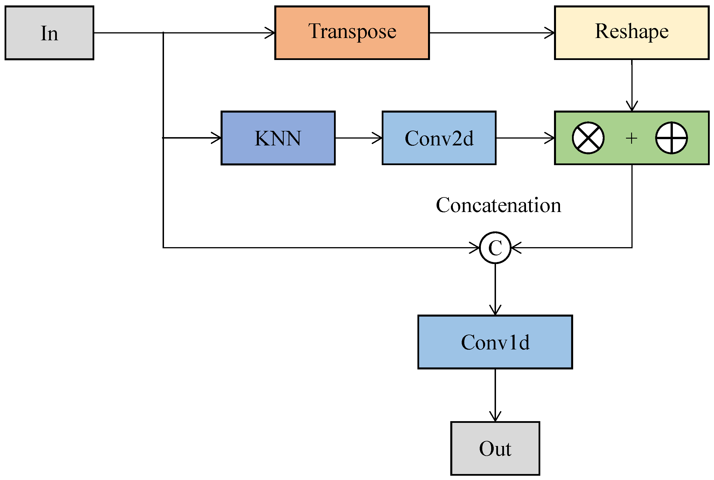
ExtractA module: Based on the first principle, we developed the ExtractA module to extract effective features, inspired by Lin et al. [14]. ExtractA solves the issues of the disorder and irregularity in point clouds. In Figure 2, the operations of reshape and transpose are to change feature dimensions; the ⨂ is the operation of point multiplication; the ⨁ is the summation operation. We constructed a local area with each point p j and j = { 1 , . . . , n } , relying on KNN. The construction process is as follows:
  • Assume that each point p j is a center point;
  • Calculate the distance value between the center point and neighboring points in a 3D coordinate system;
  • Sort these distance values in the order of smallest to largest;
  • Select the top M points ( p k , where k = { 1 , . . . , m } ) according to the sorted results;
  • Construct a local region containing the center point and first M points near it.
This construction process improves the accuracy of feature extraction. The reason for this is that when the 3D distance between two points is smaller than a specified threshold, they can be classified into one category. The distance among points belonging to the same category is relatively small, while the distance between points of different categories is relatively large, that is the distance among points can reflect their category relationship. The distance can also reflect the spatial relationship among points.
After the above construction, we calculated the local feature L p j of the center point p j :
L p j = p j , p k N ( p j , p k ) C 2 ( d ( p j , p k ) ) · F p k 0 ,
where N ( p j , p k ) is a local region; p j is a center point; p k is the neighboring point near p j ; d ( p j , p k ) is the distance between p j and p k in 3D coordinates; C 2 is a 2D convolution with weight sharing; F p k 0 is the feature of the neighboring point p k . Equation (8) is depicted in the second row of Figure 2. In this equation, the multiplication corresponds to the operation ⨂ in the figure; the summation corresponds to the operation ⨁ in the figure.
Equation (8) shows how the disorder and irregularity in point clouds are overcome. In detail, the feature F p k 0 of the neighboring points is only related to points and has no relationship with the order of points. The weight C 2 ( d ( p j , p k ) ) has no relationship with the order of points. The output value of the summation operation does not change with the order of points. Thus, the local feature L p j is only related to the center and neighboring points, and it has no relationship with the order of the input point clouds.
Then, we combined the features of the center and local points:
F p j 1 = C 1 ( C a t ( p j , p k ) ) ,
where F p j 1 denotes the new feature of the center point p j ; p k (k = { 1 , . . . , m } ) is the neighboring point near p j ; C a t represents the concatenation operation in Figure 2; C 1 denotes a 1D convolution. The concatenation avoids that centroid features are not considered. The 1D convolution is to re-extract the concatenated features. Therefore, F p j 1 contains the features of the center and neighboring points and overcomes the shortcomings of prior methods that only extract single features.
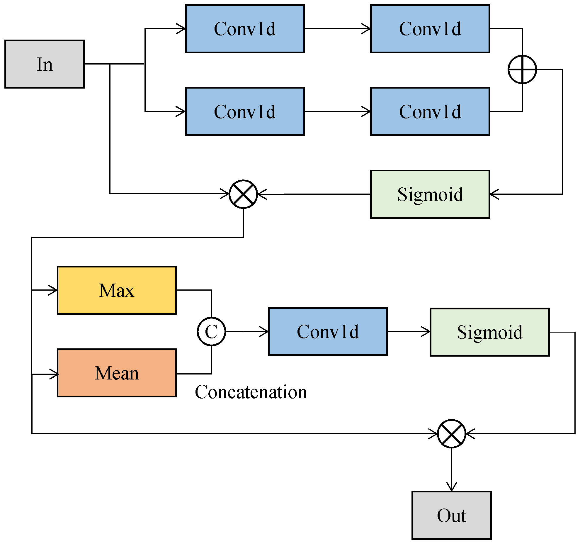
AttenA module: As shown in Figure 3, relying on the second principle, we enhanced the representation ability of ExtractA along spatial and channel dimensions, inspired by Woo et al. [16]. The channel dimension part is shown in the upper two lines of Figure 3; the spatial dimension part is depicted in the bottom two lines of this figure. In the channel dimension part, the purpose of the 1D convolutions is to extract information along two different directions. Then, we added the outputs of 1D convolutions from two different directions, as shown in the upper two lines of Figure 3. The accumulated value was normalized with a sigmoid function, which guided adaptive and accurate selection. The normalized value and the input were multiplied for the broadcast of attention values.
The output of the above channel dimension part was used as the input of the spatial dimension part. Specifically, based on the output, the operations of average-pooling and max-pooling were performed, and their outputs were concatenated for effective features. Relying on the concatenation values, we encoded the location that was suppressed or emphasized with spatial attention generated by the last 1D convolution, shown in Figure 3. Then, we normalized attention values from the 1D convolution by a sigmoid function. Finally, we multiplied the normalized values and the output of the above channel dimension part to broadcast the attention values again.
The AttenA module effectively makes information flow in EffNet. The spatial and channel dimension parts enhance the representation ability of ExtractA along the spatial and channel dimensions. The applications of 1D convolutions allow more useful features to be extracted by AttenA. This improves OCS recognition. In addition, the AttenA module has low computational complexity, as its multiply-and-accumulate operations (MACs) are approximately zero compared with the MACs of EffNet.
AttenB module: AttenB is based on the third principle in [17] with channelwise and spatialwise statistics. As shown in the upper part of Figure 4, we obtained channelwise statistics through a global averaging pooling “Avg-Pool” following Zhang et al. [17]. Thus, the global information of points was embedded. Then, a parameter function was adopted for the extraction of channel attention. The outputs of the parameter function were used as the inputs of a sigmoid function. The sigmoid function was employed for normalization and feature refinement. To broadcast channel attention values, we multiplied the normalized values from the sigmoid function and the outputs of the branch In 1 . Through the above steps, the interchannel relationship was explored.
To acquire spatialwise statistics, we employed group normalization to process the branch In 2 . The outputs of group normalization were used as the inputs of a parameter function. The purpose of the parameter function is spatial attention extraction. To refine the features, we adopted the outputs of the parameter function as the inputs of a sigmoid function. The values from the sigmoid function and the outputs of the branch In 2 were also multiplied for the broadcast of channel attention values. With these steps, the interspatial relationship was explored. Then, we concatenated the outputs of the upper and lower parts of Figure 4 for information fusion.
As features from the concatenation operation are discrete, we aggregated them in accordance with Zhang et al. [17]. Along a channel dimension, channel shuffles were performed for the exchange of information among different subfeatures of EffNet. The efficiency of AttenB was improved by grouping the channel dimension features into various subfeatures and processing them simultaneously. The AttenB module has fewer parameters and is more lightweight than the AttenA module, but AttenA extracts more features. With these modules, we completed different tasks in point cloud segmentation by constructing EffNet. We describe the detailed design process of EffNet as follows.
As depicted in Figure 5, we aggregated ExtractA, AttenA, and AttenB and built EffNet to segment point clouds for OCS recognition. The “depthwise” in this figure represents the depthwise separable 1D convolution. We employed depthwise separable 1D convolutions instead of original 1D convolutions in EffNet to reduce the model and computational complexity. The depthwise layer was used in the last layer of the second ExtractA module, as listed in the first row of Figure 5. The second and third rows also have a depthwise layer before each AttenB module. The depthwise layers reduced the parameters and MACs with group convolutions. Thus, the model and computational complexities were decreased. We adopted a ReLU layer after each depthwise layer or original convolutions to increase the nonlinear relationship in EffNet.
The input and output of EffNet are, respectively, denoted by In and out . The input and output of each module are also represented by In and out , respectively, below. Each input point consists of 3D feature dimensions. The ExtractA module was used for feature extraction, while overcoming the challenges of the disorder and irregularity in point clouds. To suppress redundant features and enhance important ones, we combined the ExtractA module with the AttenA module. The inputs of each ExtractA module consisted of the combination of the original input In and the outputs of AttenA. Through the process, the jump connection was formed. The following concatenation structures also make up the jump connection.
To further exchange point cloud features, we adopted the AttenB module, which has fewer parameters than general attention mechanisms. The output from the AttenB module was concatenated with the outputs from all AttenA modules. To extract features again, we employed a depthwise layer. The AttenB module followed closely behind for information communication. As shown in the second row of Figure 5, the output from the AttenB module was concatenated with the outputs from all AttenA modules. After the concatenation, the extracted features of point clouds contained local neighborhood information and self-information. Simultaneously, the features of different layers were combined, and the global features were obtained. Additionally, the characteristics of different layers were transferred through concatenation.
Following the first concatenation, a depthwise layer and the AttenB modules were connected sequentially for the extraction of useful features and suppression of useless features. Following the second concatenation, a depthwise layer and the AttenB modules were connected sequentially three times. The outputs of each depthwise layer and the AttenB modules were used as the input of the next ones. Then, a 1D convolution was employed to extract features. Following the 1D convolution, AttenB and a 1D convolution were adopted again to enhance valuable features. Then, the reshape operation was used to adjust the shapes of features. To predict the probability of which category each point belongs, we employed the log_softmax function used in most classification tasks. In EffNet, the direct connection helps multiple different features be extracted. The jump connection combines different features in different modules, enriching the extracted local and global features. Thus, EffNet has high efficiency, while ensuring comparable accuracy. We confirmed this effect in the experiments.

3.2. Accelerating Recognition of Point Clouds

As depicted in Figure 6, EffNet was optimized with the Auto-scheduler [19] on different architectures for the generation of high-performance tensor programs. Here, the high-performance tensor programs minimized the latency of EffNet on different architectures. Specifically, we analyzed the computation graphs of EffNet and divided them into subgraphs to obtain a series of tasks. A task is defined as a process of generating a high-performance program for a subgraph. The computation graphs of EffNet were divided into 30 tasks. The Auto-scheduler iteratively selects these tasks. It allocates time resources for them. In each iteration, a task was selected, and a program sampler generated a batch of tensor programs for each task, that is the program sampler was employed to construct a larger search space, sampling various programs. Based on the front sampled programs, the tensor program performance was auto-tuned. The performance of tensor programs was fine-tuned with an evolutionary search and a learnable cost model.
In each iteration, the performance of the tensor programs was measured on different architectures with an RPC tuning framework. We employed the platform RTX 2080 Ti GPU as a host. The host sent the batches of sampled tensor programs to different embedded devices with diverse architectures for execution. The execution time of EffNet on embedded devices was measured. The embedded devices returned the execution latency to the host, and the performance of the current program configuration parameters was evaluated on the host. Specifically, the host uses the measured performance results as inputs, trains the cost model, and executes reproduction, crossover, and mutation for configuration parameters using evolutionary search. Our model was adapted to the Pascal, Turing, or Maxwell architectures by CUDA and the ARM or x86 CPU architectures by LLVM. Then, a new tensor program with potentially higher quality was generated. Through multiple iterations of trials, we could obtain the best-performing tensor program, which refers to the program with the least latency. The best-performing tensor program was sent to embedded devices. Through the above process, we obtained the overall minimum latency of EffNet on embedded devices with different architectures.

4. Experiments

In this section, we present real experimental scenarios in Section 4.1 containing real experimental platforms, evaluation metrics, and datasets. In Section 4.2, EffNet is compared with the state-of-the-art on accuracy. In Section 4.3, the model and computational complexities of EffNet are evaluated. In Section 4.4, the latency of EffNet before and after optimization is assessed on different devices. The model latency under different tuning times is also evaluated. In Section 4.4, the visualized results of EffNet are compared with others.

4.1. Real Experimental Scenarios

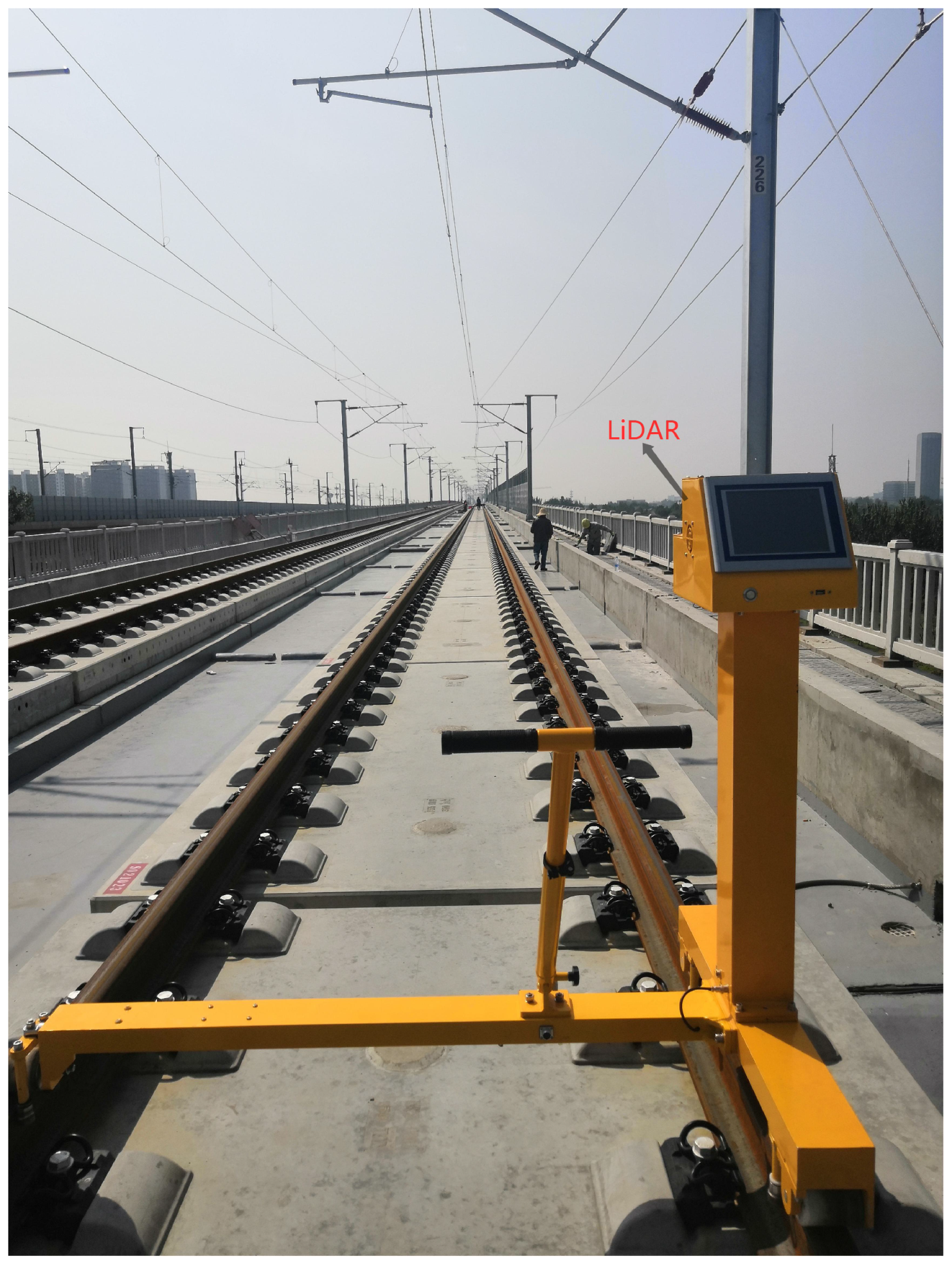
Experimental platforms and metrics: We conducted experiments in real scenarios, as listed in Figure 7. Here, the inference of the original and optimized EffNet was performed on TX2 with Max-N mode on an inspection robot. This robot can also be equipped with other popular embedded devices, such as the UP Board CPU, Nano CPU, TX2 CPU, or Nano GPU. The inspection robot walks with LiDAR that generates the point cloud data of an OCS. The data were leveraged as ground truths. The data were also employed as the inputs of our models. Based on the inputs of real scenarios, the original and optimized EffNet networks predicted the recognition results of an OCS. The results contained the comparison of the intersection over union (IoU) of each category, number of parameters/MACs, mean accuracy, latency, and precision of each category. Apart from parameters/MACs and latency, other indicators are better the higher they are. To validate the results, we compared them with similar methods, as shown in the following tables and figures.
Datasets: The OCS recognition dataset [14] was employed for model training on the RTX 2080 Ti GPU and model testing on different devices. The dataset contains point clouds generated by 2D SICK LiDAR (LMS511-20100 PRO) installed on an inspection robot. The LMS511-20100 PRO LiDAR can accurately measure the size and distance of objects. It is mainly used when high measurement accuracy is required outdoors. The measurement of the LiDAR device can achieve millimeter accuracy. When measuring distance, it filters out external interfering objects, such as dust and insects. In addition, it is small in size and light in weight. Its maximum measurement range is 80 m, and its maximum field of view is 190 . We set the scanning frequency of the LiDAR device to 25 Hz, the angular resolution to 0 . 1667 , and the scanning angle range to 90 180 . These parameters can also be set to other values. More detailed characteristics of the LiDAR device are shown on the website (https://www.sick.com/us/en/detectionandrangingsolutions/2dlidarsensors/lms5xx/lms51120100pro/p/p216240, accessed on 20 July 2021).
The robot controlled the start and end of measurement by embedded devices such as Jetson TX2. The walking speed of the robot carrying the LiDAR device was 1 m/s. While moving over rails, the robot used an odometer to continuously record the displacement of the LiDAR sensor. An odometer is relatively stable compared with a global navigation satellite system (GNSS) positioning device. In detail, when the robot carrying an odometer passes through tunnels, the odometer can still record the displacement. On the contrary, the signal of a GNSS positioning device is easily blocked in tunnels. Then, the displacement may not be recorded accurately by the GNSS positioning device in tunnels. In addition, GNSS positioning devices are extremely susceptible to electromagnetic interference. Therefore, we employed an odometer to record the displacement of the LiDAR device along the rails.
The scanning planes of the LMS511-20100 PRO LiDAR device were perpendicular to the rails, facing the OCS [28]. The scanning direction of LiDAR was used as the XY direction, and the moving direction of LiDAR was employed as the Z direction. Thus, the 3D data were formed and denoised by the dataset [14], where Lin et al. marked 16 km of the LiDAR data. They also averaged and summed the 3D coordinate values of several frames of data near the current frame. The reason for this is that adjacent frames are nearly identical, and the average and sum operations can reduce abnormal data fluctuations. Additionally, the dataset was divided into training and testing datasets. The training and testing datasets had 1,292,483 and 314,714 points, respectively. Their point densities were respectively 1052 points / m 2 and 1003 points / m 2 .

4.2. Evaluating the Accuracy Results

The precision/IoU in each category and mean accuracy of EffNet were compared with those of the state-of-the-art, as listed in Table 1. Here, the best results are in bold; PointNet++ (MSG) or (SSG), respectively, refer to PointNet++ with multiscale grouping (MSG) or single-scale grouping (SSG). For a fair comparison, the neighboring points of the KNN were set to be the same as those of the latest work [14,25]. Our method outperformed others on multiple categories of OCS recognition. Specifically, our precision was slightly higher than that of [14] in the categories of the steady arm, cantilever, pole, registration arm, dropper, insulator, contact wire, and catenary wire. Our IoU was respectively at least 3.22%, 0.05%, 3.10%, 1.89%, 2.01%, and 0.23% higher than that of the research [25] in the categories of the steady arm, pole, cantilever, registration arm, insulator, and catenary wire. Our mean accuracy of IoU was also at least 1.13% higher than that of other methods. In summary, our methods had the best accuracy for OCS recognition.

4.3. Evaluating the Number of Parameters and MACs

Evaluating the number of parameters: As depicted in Figure 8, to measure the model complexity, we calculated the number of parameters. In the figure, “[M]” represents 10 6 . The number of parameters has no relationship with the inputs. The comparison demonstrated that our model complexity is lower than that of other methods. For example, compared with the parameters of the recent research [14], ours are 40.00% fewer. EffNet has 55.17% fewer parameters than the classic study [11]. EffNet has at least 9.30% fewer parameters than the work [12]. These results denote that our model complexity is lower. The optimization of EffNet does not change the model complexity. Then, we evaluated the computational complexity of EffNet as follows.
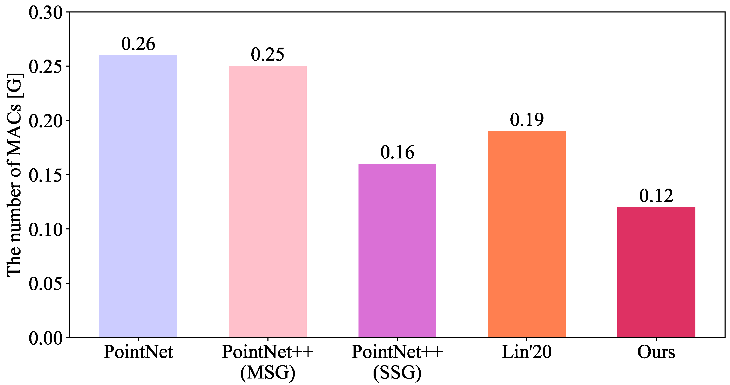
Evaluating the number of MACs: As shown in Figure 9, to measure the computational complexity of the models, we calculated the number of MACs. In the figure, “[G]” represents 10 9 . For a fair comparison, 300 point cloud points were employed as the inputs of all methods in this figure. The comparison showed that our computational complexity is lower than that of other studies. For instance, our MACs are 36.84% fewer than those of the recent work [14]. Our MACs are also 53.85% fewer than those of the classic method [11]. In short, compared with other similar methods, the MACs of EffNet are fewer, that is our computational complexity is low, and EffNet is lightweight. The optimization of EffNet does not change the computational complexity, but reduces the latency. The latency of EffNet was further evaluated on different platforms as follows.

4.4. Evaluating the Latency on Different Platforms

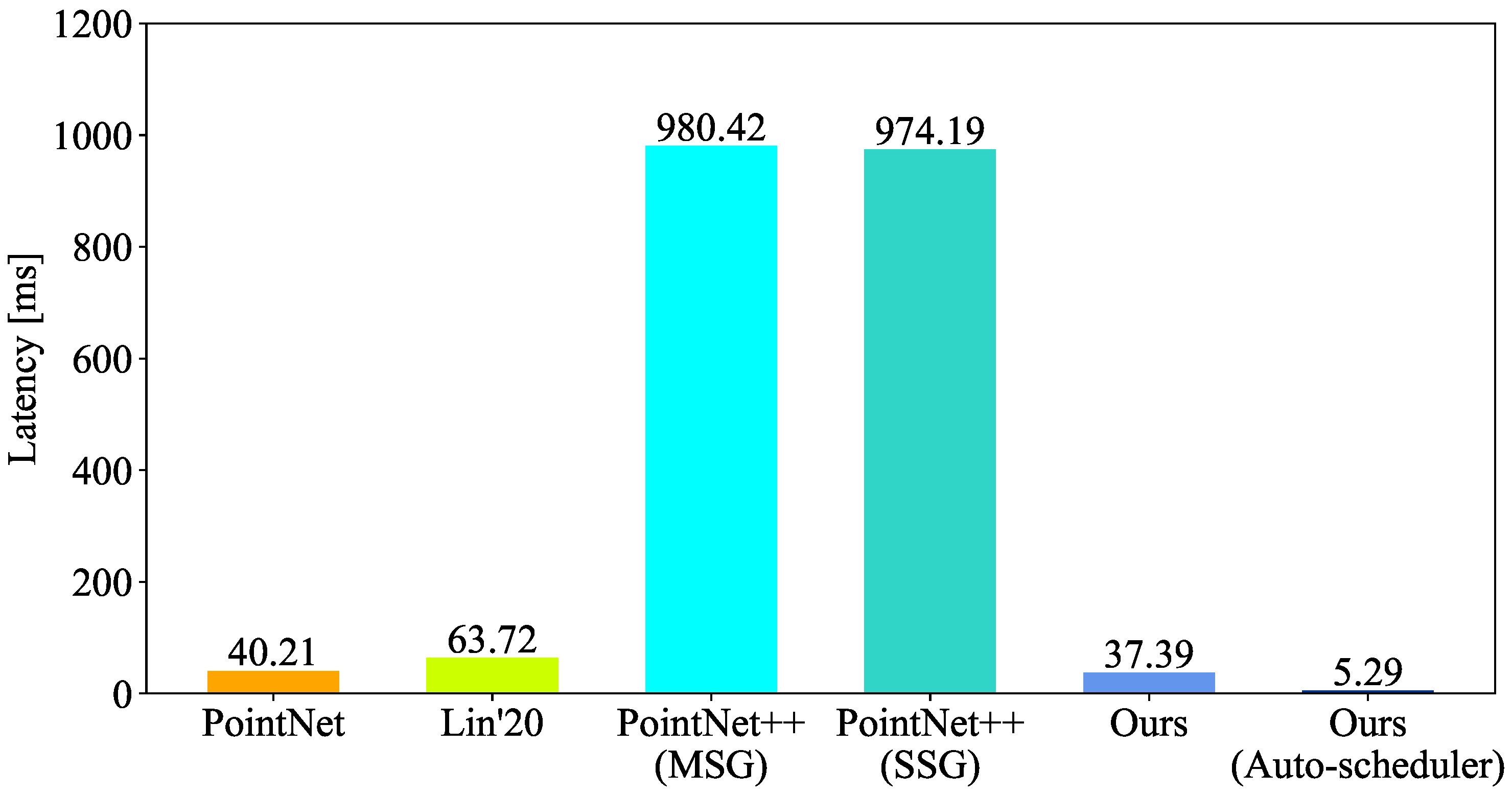
Evaluating the latency on the RTX GPU: As shown in Figure 10, our latency was compared with the state-of-the-art on the RTX 2080 Ti GPU. The comparison methods were implemented, and their latency was measured. In this figure, “Ours” and “Ours (Auto-scheduler)”, respectively, represent the latency of the original and optimized EffNet networks on the RTX 2080 Ti GPU. The inputs of all models were 1000 point cloud points. The dimension of each point was three. The unit of latency was milliseconds. The following comparison was also set up the same as this. Before optimizing EffNet, we have at least 93.64% less latency than the work [12]. The latency of the original EffNet is at least 11.23% lower than other methods [11,14]. When optimizing EffNet, we set the maximum number of trials to 10,000 on the RTX 2080 Ti GPU. We used the latency corresponding to the maximum number of tuning. After optimization, EffNet decreases the latency by 91.97%, while its accuracy is the same as before optimization on the RTX GPU. The latency of the optimized EffNet is at least an order of magnitude lower than similar recognition methods. Then, we evaluated the latency of EffNet before and after its optimization on embedded devices with different architectures.
Evaluating the latency on the TX2 GPU: We compared the latency of the original and optimized EffNet networks with the state-of-the-art on the TX2 GPU. As depicted in Figure 11, “Ours (Auto-scheduler)” and “Ours”, respectively, represent the latency of the optimized and original EffNet on the TX2 GPU. The same expression is used in the following figures, which show the comparison on other embedded devices. The maximum number of trials was set to 10,000 for optimization on the TX2 GPU and the following embedded devices. We adopted the latency corresponding to the maximum number of tuning. The optimized EffNet has at least 99.46% lower latency than the prevalent PointNet++ (MSG) or (SSG). Compared with other similar studies in the figure, the optimized EffNet has at least 86.84% less latency. The optimized EffNet reduces the latency by 85.85%, while its accuracy is the same as before optimization on the TX2 GPU. Compared with the others, the latency of the optimized EffNet is an order of magnitude less. Therefore, the optimized EffNet is efficient whether on the TX2 GPU or RTX GPU. We evaluated the latency on other embedded architectures below.
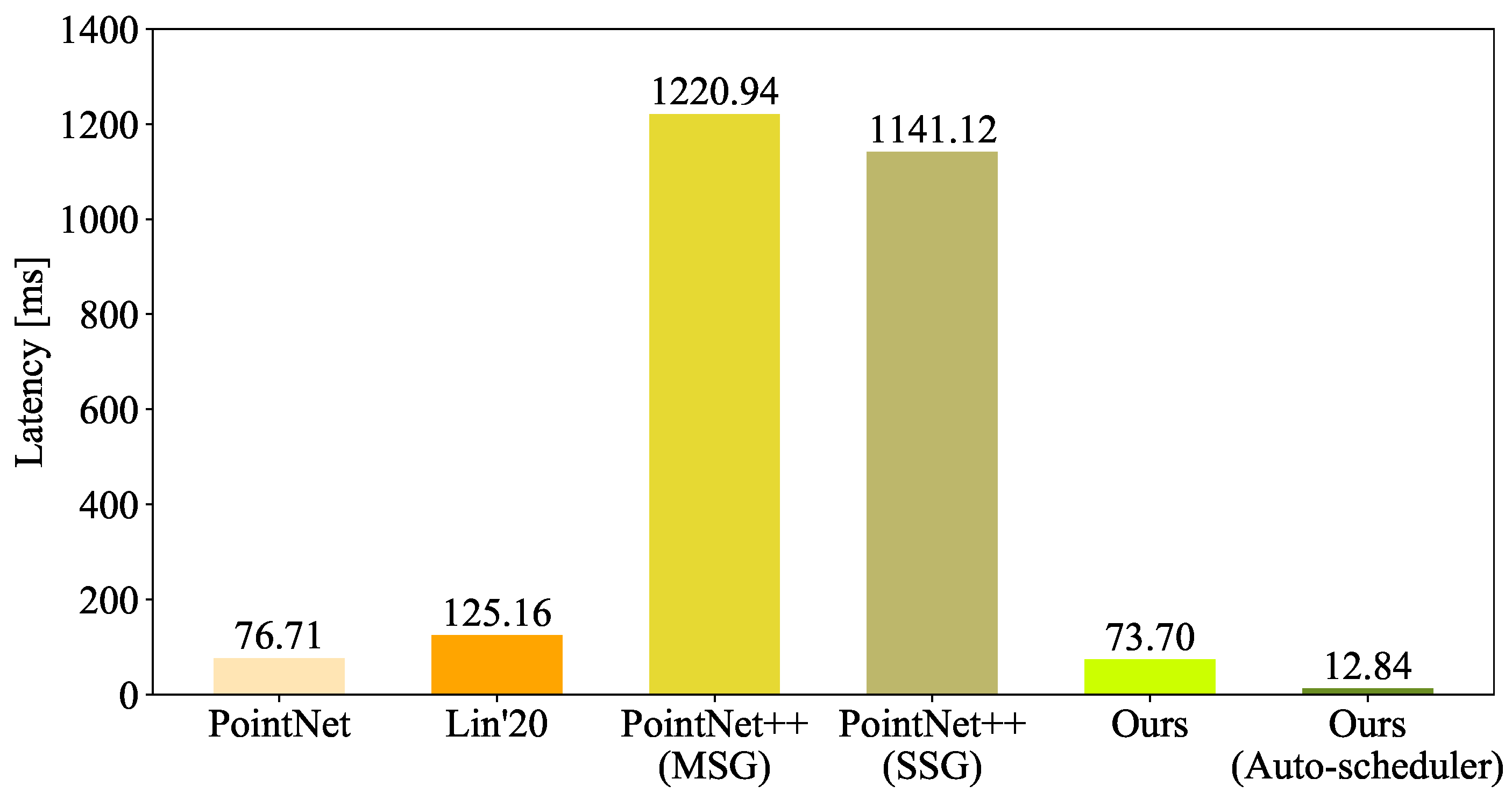
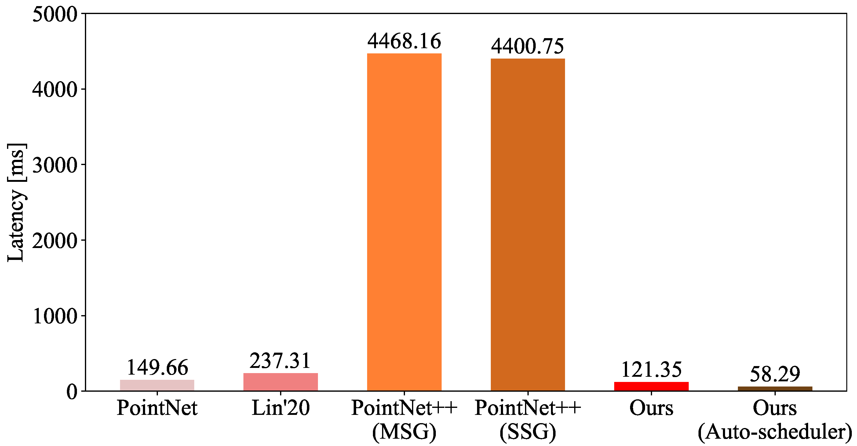
Evaluating the latency on the TX2 CPU: As shown in Figure 12, a significant difference is presented between our methods and other similar technologies on the Jetson TX2 CPU. In the figure, the original EffNet has at least 97.28% less latency than the classic work [12]. The optimized EffNet has at least 64.67% lower latency than the others. It decreases the latency by 56.47% while keeping the accuracy unchanged before and after optimization on the TX2 CPU. What is striking in the figure is that the optimized EffNet reduces the latency by an order of magnitude on the TX2 CPU. Generally speaking, the higher the accuracy, the more complex the model/computation is, and the higher the latency. However, our accuracy is slightly higher, the model and computational complexities are lower, and the latency is less than the others. The above comparison reports that the optimized EffNet is lightweight on the TX2 CPU, TX2 GPU, and RTX GPU. We compared the latency of different methods on the Nano GPU below.
Evaluating the latency on the Nano GPU: As shown in Figure 13, the comparison further supports the idea that our models match the Maxwell GPU architecture of the Nano GPU and outperform other similar methods in latency. In this figure, the original EffNet has 3.92% lower latency than the lightweight PointNet. Compared with the prevalent technologies [12,14], the original EffNet is at least 41.12% lower in latency. After optimization, our model decreases the latency by 82.58%, but the precision remains unchanged on the Nano GPU. The latency of our optimized EffNet is 83.26% less than that of comparison methods. Our low latency makes the fast operation of models running on the Maxwell GPU architecture a reality. The above experiment results show that the optimized EffNet is lightweight on the Nano GPU, TX2 CPU, TX2 GPU, or RTX GPU. We evaluated the latency of the models on the Nano CPU below.
Evaluating the latency on the Nano CPU: As depicted in Figure 14, the latency of the original and optimized EffNet networks is an order of magnitude lower than others. Our models also adapt to the ARM CPU architecture on the Nano CPU. The original EffNet has 61.05% less latency than PointNet. The optimized EffNet decreases the latency by 51.97% with unchanged accuracy. Our latency after model optimization is at least 75.44% less than that of the recent approach [14]. The comparison fully demonstrated that our methods are efficient and suitable for embedded devices, such as the Nano CPU, Nano GPU, TX2 CPU, TX2 GPU, or RTX GPU. We evaluated the results on the UP Board CPU as follows.
Evaluating the latency on the UP Board CPU: As shown in Figure 15, we compared the proposed approaches with the state-of-the-art on the UP Board CPU. The comparison confirmed that the optimized EffNet adapts to the Intel x86 CPU architecture on the UP Board CPU and improves the speed of OCS recognition. The original and optimized EffNet networks both outperform other technologies in latency. For example, the original EffNet network has at least 15.65% lower latency than the work [11,12,14]. The optimized EffNet reduces latency by 63.63% with stable accuracy on the UP Board CPU. The latency of the optimized EffNet is at least 69.32% lower than that of the lightweight study [11]. Compared with other recent studies, the optimized EffNet has 71.90% less latency. Through all the above verification, we can conclude that the optimized EffNet is effective and efficient on different devices with different architectures. We evaluated the latency of the optimized EffNet under different tuning times below.
Evaluating the latency under different tuning times: We present the latency of the optimized EffNet under different tuning times, as depicted in Figure 16. The latency changes with the number of trials on the UP Board CPU, Nano CPU, Nano GPU, TX2 CPU, TX2 GPU, and RTX GPU. In the figure, the abscissa shows the number of trials. The ordinate presents the latency. The inputs of all models were 1000 point cloud points. The dimension of each point was three. On the UP Board CPU, Nano CPU, and TX2 CPU, the latency decreases as the number of trials increases. On the Nano GPU, TX2 GPU, and RTX GPU, when the number of trials is less than 4000, the latency reduces with increasing tuning times; when tuning times exceed 4000, the latency decreases slowly as tuning times increase. When tuning times reach 10,000, the latency is lower than that under other tuning times in this figure. Therefore, we adopted the optimized model under 10,000 tuning times and deployed it to different embedded devices as the optimized EffNet. Through multiple tunings, we could find a suitable model for embedded devices. Therefore, this figure guides the choice of the optimized EffNet under different tuning times. We evaluated the visualized results of the optimized EffNet as follows.

4.5. Evaluating the Visualized Results

A visualization of the comparison methods is shown in Figure 17. We obtained the visualization results by testing the optimized EffNet in real experimental scenarios. In the figure, different colors in the rightmost position indicate different predicted components. The boxes represent the deviation between the comparison methods and ground truths. The comparison demonstrated that the optimized EffNet outperforms others. For instance, the visualization of the optimized EffNet is closer to that of the ground truths. The comparison research [25] mistook a registration arm for a catenary wire, while our prediction is similar to the ground truths. When recognizing a shoulder, our method has a smaller deviation than the others. In fact, the larger the number of neighboring points in a local area, the better the recognition. We set the number to 16, while Qi et al. [12] set it to 32. Thus, we achieved accurate prediction with a smaller number of neighboring points. Additionally, the recent work [12] had errors in the prediction of the steady arm and cantilever, while our estimation is closer to the ground truths. In summary, the optimized EffNet achieves more accurate OCS recognition than the others.

5. Conclusions

To segment point clouds for OCS recognition in complex high-speed railway scenarios, we developed a lightweight neural network EffNet containing ExtractA, AttenA, and AttenB. To further accelerate EffNet and match it with different architectures, we optimized it using a generation framework of tensor programs. The optimized EffNet adapts to diverse architectures of different devices such as the NVIDIA TX2 CPU, RTX 2080 Ti GPU, Nano GPU, Nano CPU, UP Board CPU, and TX2 GPU. Extensive experiments confirmed that our methods are effective and efficient. Compared with other methods, EffNet has at least a 0.57% higher mean accuracy, with 9.30% and 25.00% lower model and computational complexities, respectively. The optimization did not change the precision or model and computational complexity. The optimized EffNet has at least 92.87%, 83.26%, 69.32%, 18.85%, 61.05%, and 86.84% lower latency on the RTX 2080 Ti GPU, Nano GPU, UP Board CPU, TX2 CPU, Nano CPU, and TX2 GPU, respectively, than the others. Our latency measurement under different tuning times guided the choice of models with high speed. Our visualization also outperformed others in real high-speed railway scenarios. To the best of our knowledge, this paper presents a fast model with lower computational/model complexity and slightly higher accuracy than existing methods for OCS recognition. The optimized model reduces inference latency by an order of magnitude in complex high-speed railway scenarios, while matching different embedded systems. As we emphasize algorithms, the same dataset was adopted to validate algorithm performance; LiDAR point density and digital elevation models were not considered. We will make up for this shortcoming in future work.

Author Contributions

Conceptualization, S.L. (Siping Liu), X.T., S.L. (Shuai Lin), C.X. and R.L.; methodology, S.L. (Siping Liu), S.L. (Shuai Lin), and X.T.; data curation, L.C., X.T. and S.L. (Shuai Lin); software, S.L. (Siping Liu), X.T., S.L. (Shuai Lin), and L.C.; investigation, L.C., S.L. (Shuai Lin), and C.X.; validation, S.L. (Siping Liu) and X.T.; writing—original draft preparation, S.L. (Siping Liu); writing—review and editing, S.L. (Siping Liu) and X.T.; supervision, R.L. and C.X.; funding acquisition, R.L. and C.X. All authors have read and agreed to the published version of the manuscript.

Funding

This work was supported by the National Natural Science Foundation of China under Grant No. 61772185 and 61932010.

Institutional Review Board Statement

Not applicable.

Informed Consent Statement

Not applicable.

Data Availability Statement

Data available on request due to restrictions eg privacy or ethical. The data presented in this study are available on request from the corresponding author. The data are not publicly available due to restrictions e.g., their containing information that could compromise the privacy of research participants.

Conflicts of Interest

The authors declare no conflict of interest.

References

  1. Tian, Y.; Chen, L.; Song, W.; Sung, Y.; Woo, S. DGCB-Net: Dynamic Graph Convolutional Broad Network for 3D Object Recognition in Point Cloud. Remote Sens. 2021, 13, 66. [Google Scholar] [CrossRef]
  2. Pierdicca, R.; Paolanti, M.; Matrone, F.; Martini, M.; Morbidoni, C.; Malinverni, E.S.; Frontoni, E.; Lingua, A.M. Point Cloud Semantic Segmentation Using a Deep Learning Framework for Cultural Heritage. Remote Sens. 2020, 12, 1005. [Google Scholar] [CrossRef] [Green Version]
  3. Arastounia, M. Automated Recognition of Railroad Infrastructure in Rural Areas from LIDAR Data. Remote Sens. 2015, 7, 14916–14938. [Google Scholar] [CrossRef] [Green Version]
  4. Tang, Y.C.; Li, L.J.; Feng, W.X.; Liu, F.; Zou, X.J.; Chen, M.Y. Binocular vision measurement and its application in full-field convex deformation of concrete-filled steel tubular columns. Measurement 2018, 130, 372–383. [Google Scholar] [CrossRef]
  5. Kang, G.; Gao, S.; Yu, L.; Zhang, D. Deep Architecture for High-Speed Railway Insulator Surface Defect Detection: Denoising Autoencoder With Multitask Learning. IEEE Trans. Instrum. Meas. 2019, 68, 2679–2690. [Google Scholar] [CrossRef]
  6. Tu, X.; Xu, C.; Liu, S.; Xie, G.; Li, R. Real-Time Depth Estimation with an Optimized Encoder-Decoder Architecture on Embedded Devices. In Proceedings of the IEEE 21st International Conference on High Performance Computing and Communications, Zhangjiajie, China, 10–12 August 2019; pp. 2141–2149. [Google Scholar] [CrossRef]
  7. Wei, X.; Jiang, S.; Li, Y.; Li, C.; Jia, L.; Li, Y. Defect Detection of Pantograph Slide Based on Deep Learning and Image Processing Technology. IEEE Trans. Intell. Transp. Syst. 2020, 21, 947–958. [Google Scholar] [CrossRef]
  8. Han, Z.; Yang, C.; Liu, Z. Cantilever Structure Segmentation and Parameters Detection Based on Concavity and Convexity of 3-D Point Clouds. IEEE Trans. Instrum. Meas. 2020, 69, 3026–3036. [Google Scholar] [CrossRef]
  9. Pastucha, E. Catenary System Detection, Localization and Classification Using Mobile Scanning Data. Remote Sens. 2016, 8, 801. [Google Scholar] [CrossRef] [Green Version]
  10. Tu, X.; Xu, C.; Liu, S.; Li, R.; Xie, G.; Huang, J.; Yang, L.T. Efficient Monocular Depth Estimation for Edge Devices in Internet of Things. IEEE Trans. Ind. Inform. 2021, 17, 2821–2832. [Google Scholar] [CrossRef]
  11. Qi, C.R.; Su, H.; Mo, K.; Guibas, L.J. PointNet: Deep Learning on Point Sets for 3D Classification and Segmentation. In Proceedings of the IEEE Conference on Computer Vision and Pattern Recognition, Honolulu, HI, USA, 21–26 July 2017; pp. 77–85. [Google Scholar] [CrossRef] [Green Version]
  12. Qi, C.R.; Yi, L.; Su, H.; Guibas, L.J. PointNet++: Deep Hierarchical Feature Learning on Point Sets in a Metric Space. In Proceedings of the 31st International Conference on Neural Information Processing Systems, Long Beach, CA, USA, 4–9 December 2017; pp. 5099–5108. [Google Scholar]
  13. Chen, Y.; Liu, G.; Xu, Y.; Pan, P.; Xing, Y. PointNet++ Network Architecture with Individual Point Level and Global Features on Centroid for ALS Point Cloud Classification. Remote Sens. 2021, 13, 472. [Google Scholar] [CrossRef]
  14. Lin, S.; Xu, C.; Chen, L.; Li, S.; Tu, X. LiDAR Point Cloud Recognition of Overhead Catenary System with Deep Learning. Sensors 2020, 20, 2212. [Google Scholar] [CrossRef] [PubMed] [Green Version]
  15. Altman, N.S. An Introduction to Kernel and Nearest-Neighbor Nonparametric Regression. Am. Stat. 1992, 46, 175–185. [Google Scholar] [CrossRef] [Green Version]
  16. Woo, S.; Park, J.; Lee, J.Y.; Kweon, I.S. CBAM: Convolutional Block Attention Module. In Proceedings of the European Conference on Computer Vision, Munich, Germany, 8–14 September 2018; pp. 3–19. [Google Scholar] [CrossRef] [Green Version]
  17. Zhang, Q.L.; Yang, Y.B. SA-Net: Shuffle Attention for Deep Convolutional Neural Networks. In Proceedings of the IEEE International Conference on Acoustics, Speech and Signal Processing, Toronto, ON, Canada, 6–11 June 2021; pp. 2235–2239. [Google Scholar] [CrossRef]
  18. Vaswani, A.; Shazeer, N.; Parmar, N.; Uszkoreit, J.; Jones, L.; Gomez, A.N.; Kaiser, L.; Polosukhin, I. Attention is All you Need. In Proceedings of the 31st International Conference on Neural Information Processing Systems, Long Beach, CA, USA, 4–9 December 2017; Curran Associates, Inc.: Nice, France, 2017; Volume 30, pp. 6000–6010. [Google Scholar]
  19. Zheng, L.; Jia, C.; Sun, M.; Wu, Z.; Yu, C.H.; Haj-Ali, A.; Wang, Y.; Yang, J.; Zhuo, D.; Sen, K.; et al. Ansor: Generating High-Performance Tensor Programs for Deep Learning. In Proceedings of the 14th USENIX Symposium on Operating Systems Design and Implementation, Banff, AB, Canada, 4–6 November 2020; pp. 863–879. [Google Scholar]
  20. Lattner, C.; Adve, V. LLVM: A compilation framework for lifelong program analysis & transformation. In Proceedings of the International Symposium on Code Generation and Optimization, Palo Alto, CA, USA, 20–24 March 2004; pp. 75–86. [Google Scholar] [CrossRef]
  21. Garland, M.; Le Grand, S.; Nickolls, J.; Anderson, J.; Hardwick, J.; Morton, S.; Phillips, E.; Zhang, Y.; Volkov, V. Parallel Computing Experiences with CUDA. IEEE Micro 2008, 28, 13–27. [Google Scholar] [CrossRef]
  22. Vikhar, P.A. Evolutionary algorithms: A critical review and its future prospects. In Proceedings of the International Conference on Global Trends in Signal Processing, Information Computing and Communication, Jalgaon, India, 22–24 December 2016; pp. 261–265. [Google Scholar] [CrossRef]
  23. Chen, T.; Zheng, L.; Yan, E.; Jiang, Z.; Moreau, T.; Ceze, L.; Guestrin, C.; Krishnamurthy, A. Learning to Optimize Tensor Programs. In Proceedings of the Advances in Neural Information Processing Systems, Montréal, QC, Canada, 3–8 December 2018; Volume 31, pp. 3393–3404. [Google Scholar]
  24. Chen, L.; Jung, J.; Sohn, G. Multi-Scale Hierarchical CRF for Railway Electrification Asset Classification From Mobile Laser Scanning Data. IEEE J. Sel. Top. Appl. Earth Obs. Remote Sens. 2019, 12, 3131–3148. [Google Scholar] [CrossRef]
  25. Tu, X.; Xu, C.; Liu, S.; Lin, S.; Chen, L.; Xie, G.; Li, R. LiDAR Point Cloud Recognition and Visualization with Deep Learning for Overhead Contact Inspection. Sensors 2020, 20, 6387. [Google Scholar] [CrossRef] [PubMed]
  26. Ren, S.; He, K.; Girshick, R.; Sun, J. Faster R-CNN: Towards Real-Time Object Detection with Region Proposal Networks. IEEE Trans. Pattern Anal. Mach. Intell. 2017, 39, 1137–1149. [Google Scholar] [CrossRef] [PubMed] [Green Version]
  27. Wu, Y.; He, K. Group Normalization. In Proceedings of the European Conference on Computer Vision, Munich, Germany, 8–14 September 2018; pp. 3–19. [Google Scholar] [CrossRef]
  28. Chen, M.; Tang, Y.; Zou, X.; Huang, K.; Li, L.; He, Y. High-accuracy multi-camera reconstruction enhanced by adaptive point cloud correction algorithm. Opt. Lasers Eng. 2019, 122, 170–183. [Google Scholar] [CrossRef]
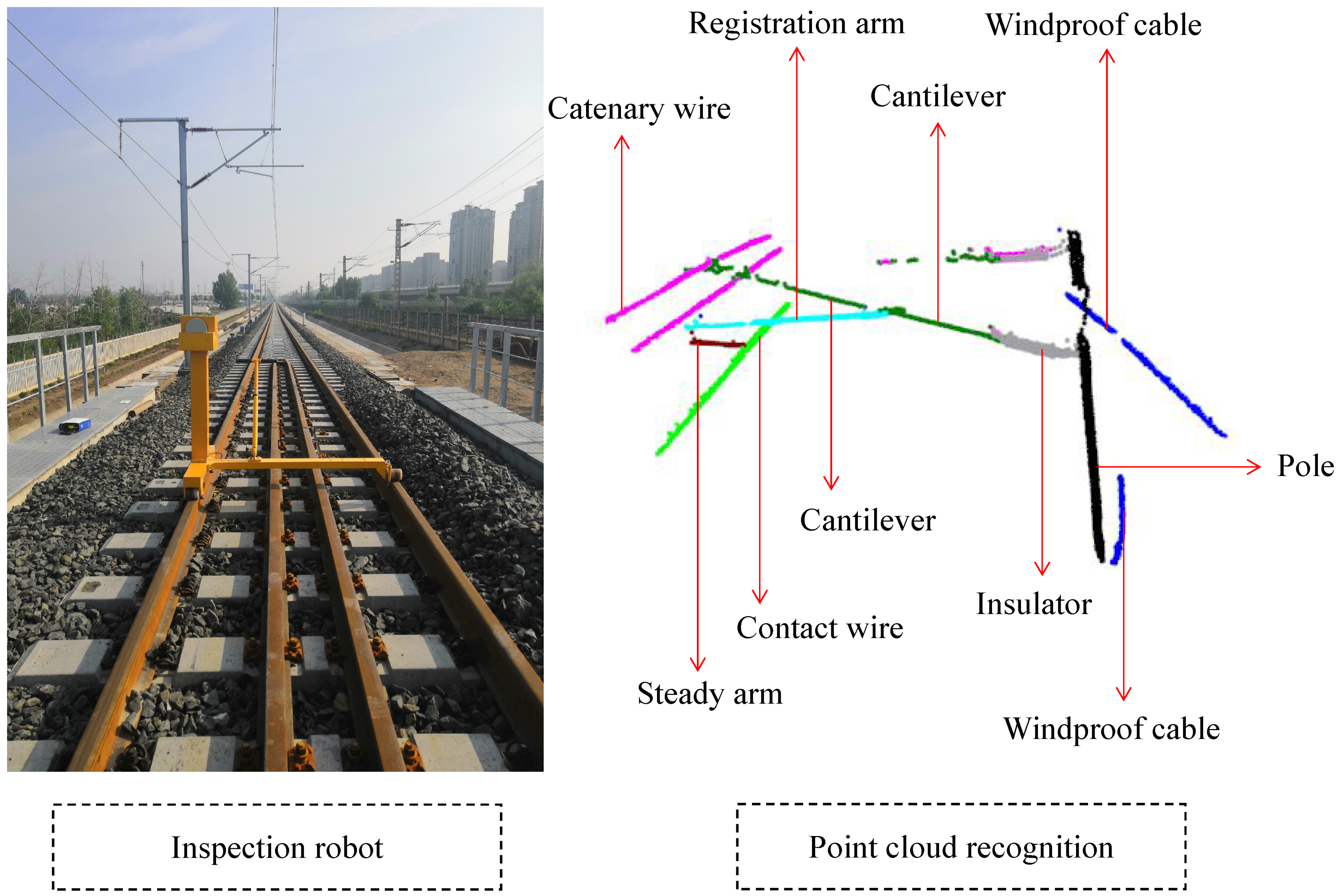
Figure 1. Recognizing an overhead contact system.
Remotesensing 13 04110 g001
Figure 2. The ExtractA module.
Remotesensing 13 04110 g002
Figure 3. The AttenA module.
Remotesensing 13 04110 g003
Figure 4. The AttenB module.
Remotesensing 13 04110 g004
Figure 5. The proposed EffNet.
Remotesensing 13 04110 g005
Figure 6. Accelerating recognition of point clouds.
Remotesensing 13 04110 g006
Figure 7. The actual inspection robot.
Remotesensing 13 04110 g007
Figure 8. Evaluating the number of parameters.
Remotesensing 13 04110 g008
Figure 9. Evaluating the number of MACs.
Remotesensing 13 04110 g009
Figure 10. Comparison of the latency on the RTX GPU.
Remotesensing 13 04110 g010
Figure 11. Comparison of the latency on the TX2 GPU.
Remotesensing 13 04110 g011
Figure 12. Comparison of the latency on the TX2 CPU.
Remotesensing 13 04110 g012
Figure 13. Comparison of the latency on the Nano GPU.
Remotesensing 13 04110 g013
Figure 14. Comparison of the latency on the Nano CPU.
Remotesensing 13 04110 g014
Figure 15. Comparison of latency on the UP Board CPU.
Remotesensing 13 04110 g015
Figure 16. Comparison of the latency under different tuning times.
Remotesensing 13 04110 g016
Figure 17. Evaluating the visualized results.
Remotesensing 13 04110 g017
Table 1. Evaluating accuracy results. Point cloud categories are C1: pole, C2: catenary wire, C3: contact wire, C4: insulator, C5: dropper, C6: steady arm, C7: registration arm, C8: cantilever.
MethodAccuracyC1C2C3C4C5C6C7C8Mean
PointNetPrecision99.7398.9999.1496.0389.6792.0293.5987.0394.52
IoU99.3498.1298.7491.6876.8482.2388.6477.8789.18
PointNet++(SSG)Precision99.8598.5799.3797.2697.2291.1295.4292.6096.42
IoU99.6597.9398.2894.4593.1583.3389.8387.8893.06
PointNet++(MSG)Precision99.8698.6199.5197.1096.9690.8095.3993.3896.45
IoU99.6498.0698.4794.2193.7284.5190.6187.7593.37
Lin et al. [14]Precision99.8099.4599.7997.3696.3995.2795.2392.8197.01
IoU99.6499.1699.6093.5991.9186.4492.1187.2393.71
Tu et al. [25]Precision99.9199.6599.8997.1897.1695.9794.7093.8797.17
IoU99.7699.5199.7594.1293.6885.6891.3888.6894.07
OursPrecision99.9199.8799.8798.9697.1395.9095.5494.7897.72
IoU99.8199.7499.7496.0193.0188.4493.1191.4395.13
Publisher’s Note: MDPI stays neutral with regard to jurisdictional claims in published maps and institutional affiliations.