
Model Specialization for the Use of ESRGAN on Satellite and Airborne Imagery


Abstract
:
1. Introduction
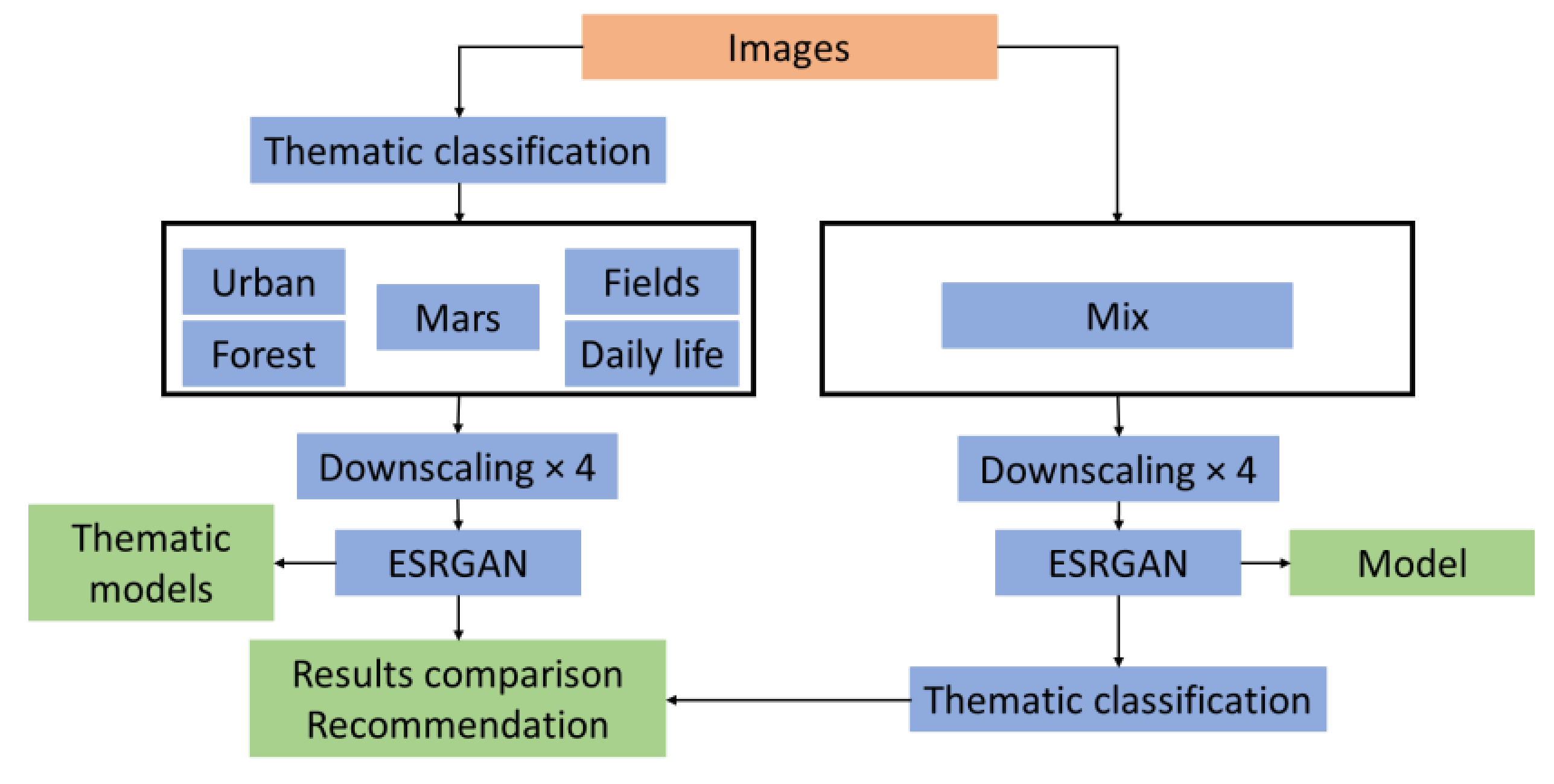
2. Materials and Methods
2.1. ESRGAN Architecture
2.2. Datasets
3. Results
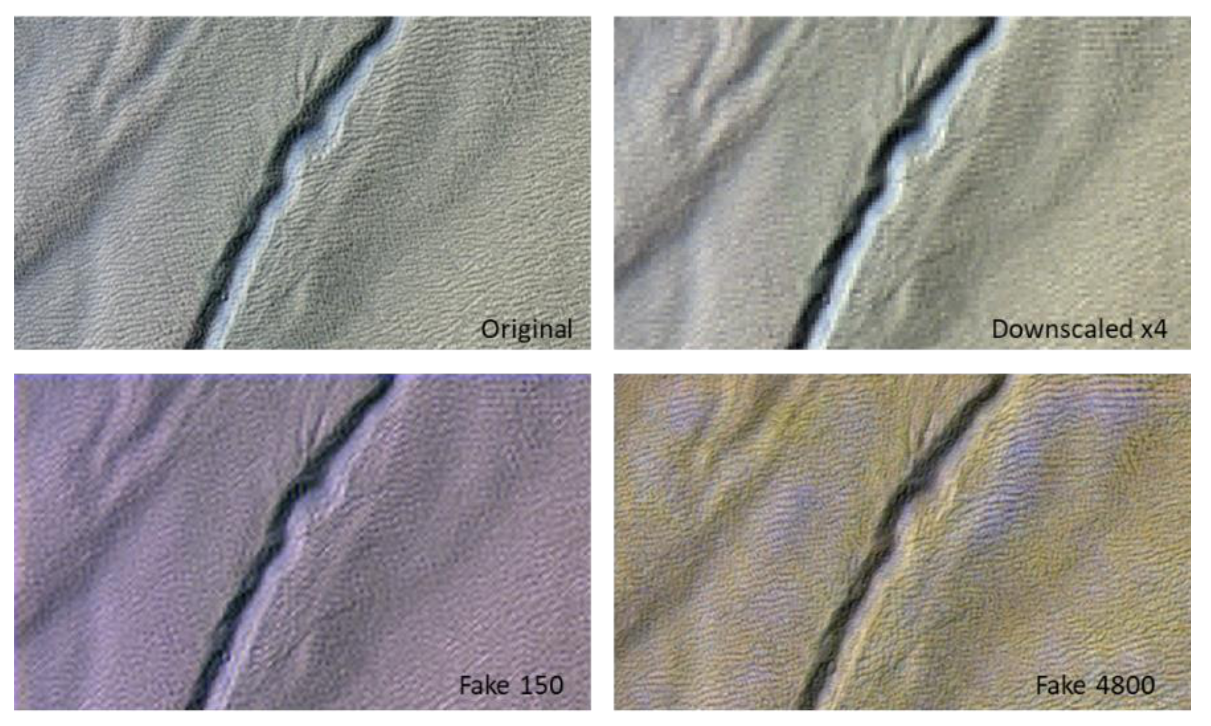
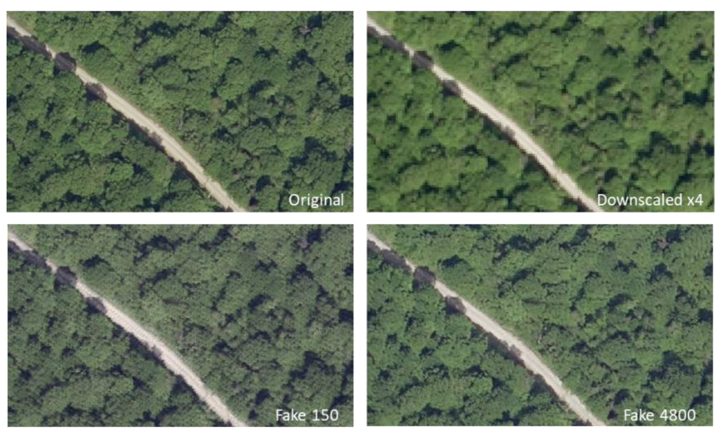
3.1. Examples of Upscaling Results
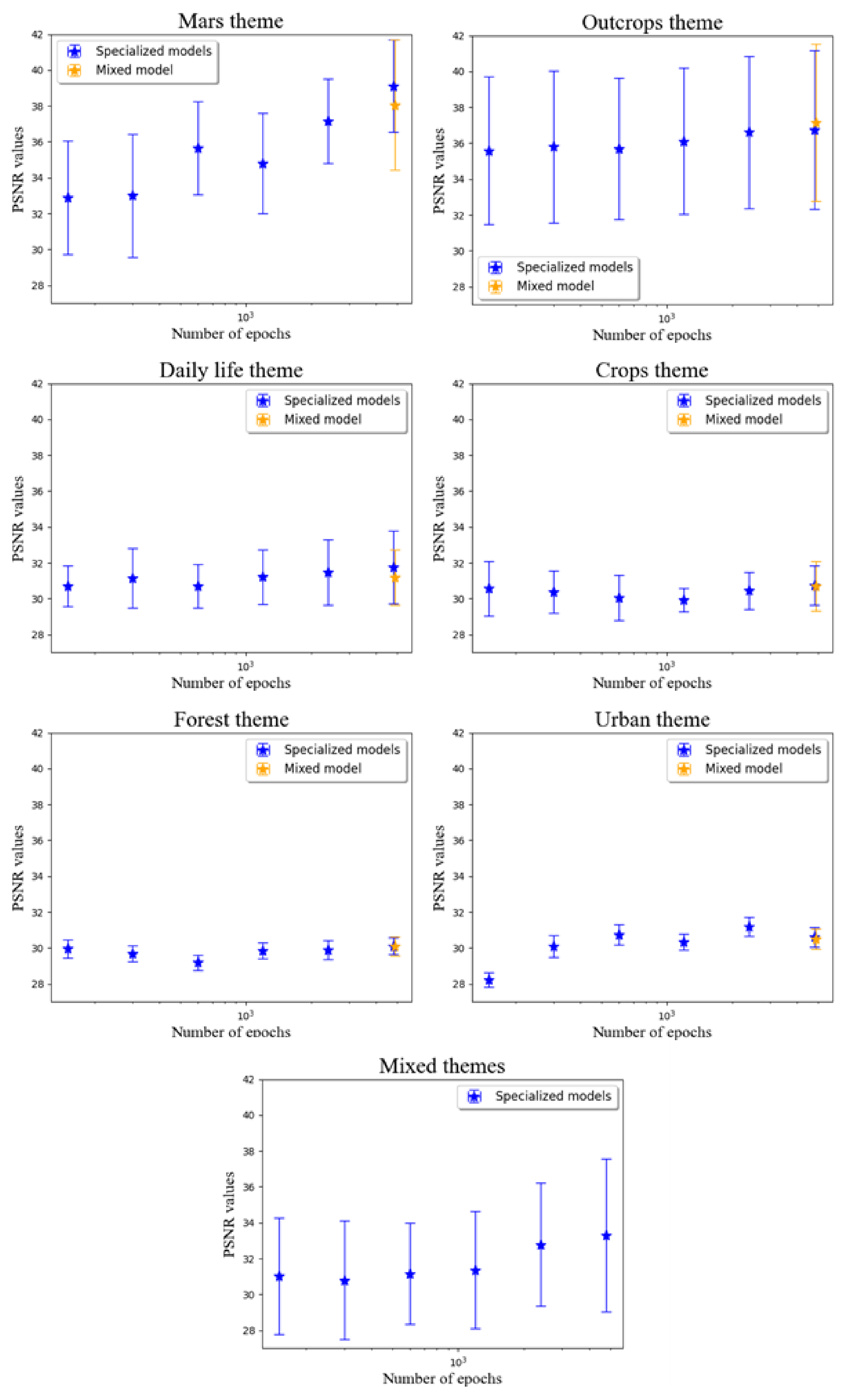
3.2. PSNR Obtained for Each Model
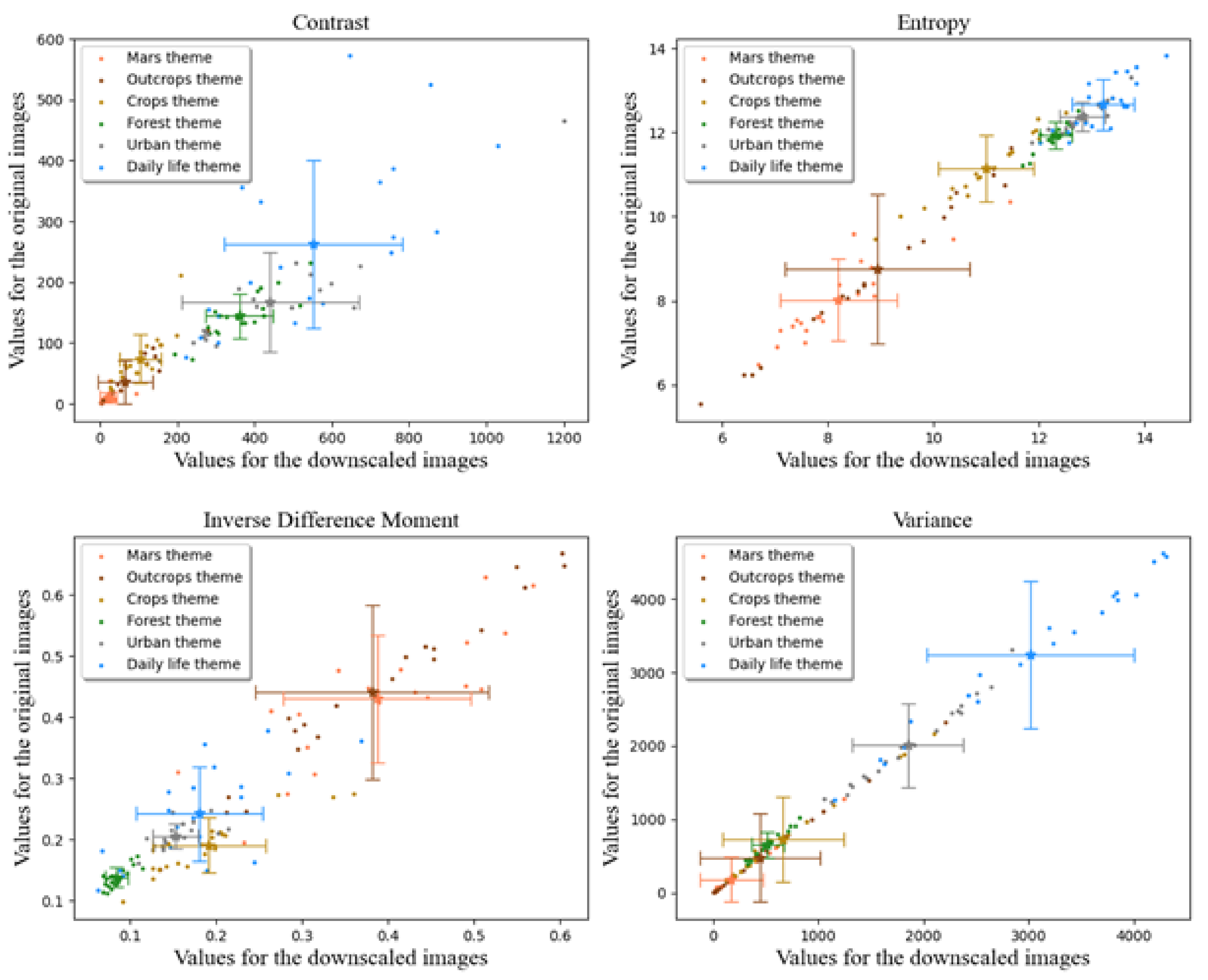
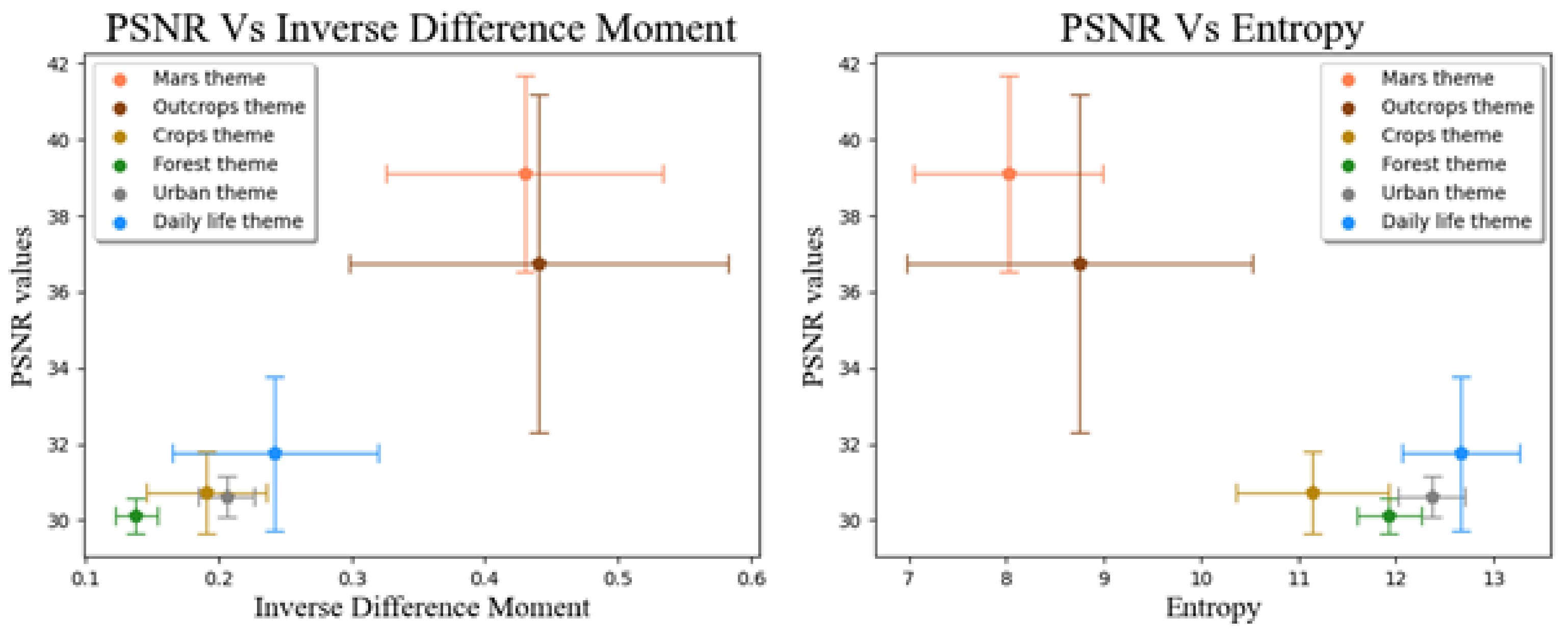
3.3. Texture Indices
4. Discussion
4.1. Image Resolution Improvement with ESRGAN
4.2. Interest in the Specialization of Examples in Learning
4.3. Texture Indices and Reconstruction of HR Images
5. Conclusions
- It is more beneficial to create a specialized ESRGAN model for a specific task, rather than trying to maximize the variability in examples.
- The ability to learn depends upon the subject matter. No recommendations can be made a priori.
- ESRGAN perform better on images with a high inverse difference moment and low entropy indices.
Author Contributions
Funding
Data Availability Statement
Acknowledgments
Conflicts of Interest
References
- Transon, J.; d’Andrimont, R.; Maugnard, A.; Defourny, P. Survey of Hyperspectral Earth Observation Applications from Space in the Sentinel-2 Context. Remote Sens. 2018, 10, 157. [Google Scholar] [CrossRef] [Green Version]
- Collin, A.M.; Andel, M.; James, D.; Claudet, J. The Superspectral/Hyperspatial Worldview-3 as the Link Between Spaceborne Hyperspectral and Airborne Hyperspatial Sensors: The Case Study of the Complex Tropical Coast. Int. Arch. Photogramm. Remote Sens. Spatial Inf. Sci. 2019, XLII-2/W13, 1849–1854. [Google Scholar] [CrossRef] [Green Version]
- Pandey, P.C.; Koutsias, N.; Petropoulos, G.P.; Srivastava, P.K.; Ben Dor, E. Land Use/Land Cover in View of Earth Observation: Data Sources, Input Dimensions, and Classifiers—a Review of the State of the Art. Geocarto Int. 2021, 36, 957–988. [Google Scholar] [CrossRef]
- Haut, J.M.; Fernandez-Beltran, R.; Paoletti, M.E.; Plaza, J.; Plaza, A. Remote Sensing Image Superresolution Using Deep Residual Channel Attention. IEEE Trans. Geosci. Remote Sens. 2019, 57, 9277–9289. [Google Scholar] [CrossRef]
- Märtens, M.; Izzo, D.; Krzic, A.; Cox, D. Super-Resolution of PROBA-V Images Using Convolutional Neural Networks. Astrodyn 2019, 3, 387–402. [Google Scholar] [CrossRef]
- Deudon, M.; Kalaitzis, A.; Goytom, I.; Arefin, M.R.; Lin, Z.; Sankaran, K.; Michalski, V.; Kahou, S.E.; Cornebise, J.; Bengio, Y. HighRes-Net: Recursive Fusion for Multi-Frame Super-Resolution of Satellite Imagery. arXiv 2020, arXiv:2002.06460. [Google Scholar]
- Lugmayr, A.; Danelljan, M.; Timofte, R. NTIRE 2021 Learning the Super-Resolution Space Challenge. In Proceedings of the 2021 IEEE/CVF Conference on Computer Vision and Pattern Recognition Workshops (CVPRW), Nashville, TN, USA, 19–25 June 2021; pp. 596–612. [Google Scholar]
- Lugmayr, A.; Danelljan, M.; Van Gool, L.; Timofte, R. SRFlow: Learning the Super-Resolution Space with Normalizing Flow. In Proceedings of the Computer Vision—ECCV 2020; Vedaldi, A., Bischof, H., Brox, T., Frahm, J.-M., Eds.; Springer International Publishing: Cham, Switzerland, 2020; pp. 715–732. [Google Scholar]
- Ayas, S. Single Image Super Resolution Using Dictionary Learning and Sparse Coding with Multi-Scale and Multi-Directional Gabor Feature Representation. Inf. Sci. 2020, 512, 1264–1278. [Google Scholar] [CrossRef]
- Dong, C.; Loy, C.C.; He, K.; Tang, X. Learning a Deep Convolutional Network for Image Super-Resolution. In Proceedings of the European Conference on Computer Vision, Zurich, Switzerland, 6–14 September 2014; p. 16. [Google Scholar]
- Kim, J.; Lee, J.K.; Lee, K.M. Accurate Image Super-Resolution Using Very Deep Convolutional Networks. In Proceedings of the 2016 IEEE Conference on Computer Vision and Pattern Recognition (CVPR), Las Vegas, NV, USA, 26 June–1 July 2016; IEEE: Manhattan, NY, USA, 2016; pp. 1646–1654. [Google Scholar]
- Yang, W.; Zhang, X.; Tian, Y.; Wang, W.; Xue, J.-H.; Liao, Q. Deep Learning for Single Image Super-Resolution: A Brief Review. IEEE Trans. Multimedia 2019, 21, 3106–3121. [Google Scholar] [CrossRef] [Green Version]
- Wang, X.; Yu, K.; Wu, S.; Gu, J.; Liu, Y.; Dong, C.; Qiao, Y.; Loy, C.C. ESRGAN: Enhanced Super-Resolution Generative Adversarial Networks. In Computer Vision—ECCV 2018 Workshops; Leal-Taixé, L., Roth, S., Eds.; Lecture Notes in Computer Science; Springer International Publishing: Cham, Switzerland, 2019; Volume 11133, pp. 63–79. ISBN 978-3-030-11020-8. [Google Scholar]
- Romero, L.S.; Marcello, J.; Vilaplana, V. Super-Resolution of Sentinel-2 Imagery Using Generative Adversarial Networks. Remote Sens. 2020, 12, 2424. [Google Scholar] [CrossRef]
- Clabaut, É.; Lemelin, M.; Germain, M. Generation of Simulated “Ultra-High Resolution” HiRISE Imagery Using Enhanced Super-Resolution Generative Adversarial Network Modeling. Online. 15 March 2021, p. 2. Available online: https://www.hou.usra.edu/meetings/lpsc2021/pdf/1935.pdf (accessed on 6 October 2021).
- Watson, C.D.; Wang, C.; Lynar, T.; Weldemariam, K. Investigating Two Super-Resolution Methods for Downscaling Precipitation: ESRGAN and CAR. arXiv 2020, arXiv:2012.01233. [Google Scholar]
- Wu, Z.; Ma, P. Esrgan-Based Dem Super-Resolution for Enhanced Slope Deformation Monitoring In Lantau Island Of Hong Kong. Int. Arch. Photogramm. Remote Sens. Spatial Inf. Sci. 2020, XLIII-B3-2020, 351–356. [Google Scholar] [CrossRef]
- Perez, L.; Wang, J. The Effectiveness of Data Augmentation in Image Classification Using Deep Learning. arXiv 2017, arXiv:1712.04621. [Google Scholar]
- Shorten, C.; Khoshgoftaar, T.M. A Survey on Image Data Augmentation for Deep Learning. J. Big Data 2019, 6, 60. [Google Scholar] [CrossRef]
- Srivastava, N.; Hinton, G.; Krizhevsky, A.; Sutskever, I.; Salakhutdinov, R. Dropout: A Simple Way to Prevent Neural Networks from Overfitting. J. Mach. Learn. Res. 2014, 15, 1929–1958. [Google Scholar]
- Raskutti, G.; Wainwright, M.J.; Yu, B. Early Stopping and Non-Parametric Regression: An Optimal Data-Dependent Stopping Rule. J. Mach. Learn. Res. 2014, 15, 335–366. [Google Scholar]
- Li, M.; Soltanolkotabi, M.; Oymak, S. Gradient Descent with Early Stopping Is Provably Robust to Label Noise for Overparameterized Neural Networks. In Proceedings of the International Conference on Artificial Intelligence and Statistics, Palermo, Sicily, Italy, 3–5 June 2020. [Google Scholar]
- Haralick, R.M.; Shanmugam, K.; Dinstein, I. Textural Features for Image Classification. IEEE Trans. Syst. Man Cybern. 1973, SMC-3, 610–621. [Google Scholar] [CrossRef] [Green Version]
- Ledig, C.; Theis, L.; Huszar, F.; Caballero, J.; Cunningham, A.; Acosta, A.; Aitken, A.; Tejani, A.; Totz, J.; Wang, Z.; et al. Photo-Realistic Single Image Super-Resolution Using a Generative Adversarial Network. arXiv 2017, arXiv:1609.04802. [Google Scholar]
- Agustsson, E.; Timofte, R. NTIRE 2017 Challenge on Single Image Super-Resolution: Dataset and Study. In Proceedings of the 2017 IEEE Conference on Computer Vision and Pattern Recognition Workshops (CVPRW), Honolulu, HI, USA, 21–26 July 2017; pp. 1122–1131. [Google Scholar]
- Lugmayr, A.; Danelljan, M.; Timofte, R. Unsupervised Learning for Real-World Super-Resolution. arXiv 2019, arXiv:1909.09629. [Google Scholar]
- Umer, R.M.; Foresti, G.L.; Micheloni, C. Deep Generative Adversarial Residual Convolutional Networks for Real-World Super-Resolution. arXiv 2020, arXiv:2005.00953. [Google Scholar]

| Spatial Resolution | Location | |
|---|---|---|
| DIV2K | Not relevant | Unknown |
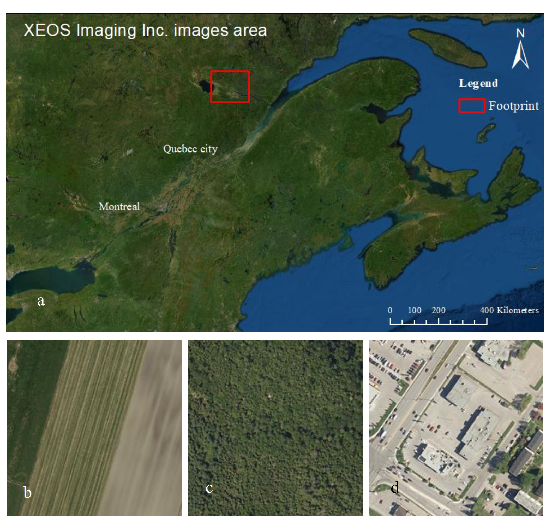
| Airborne imagery | 20 cm | Québec (Canada) |
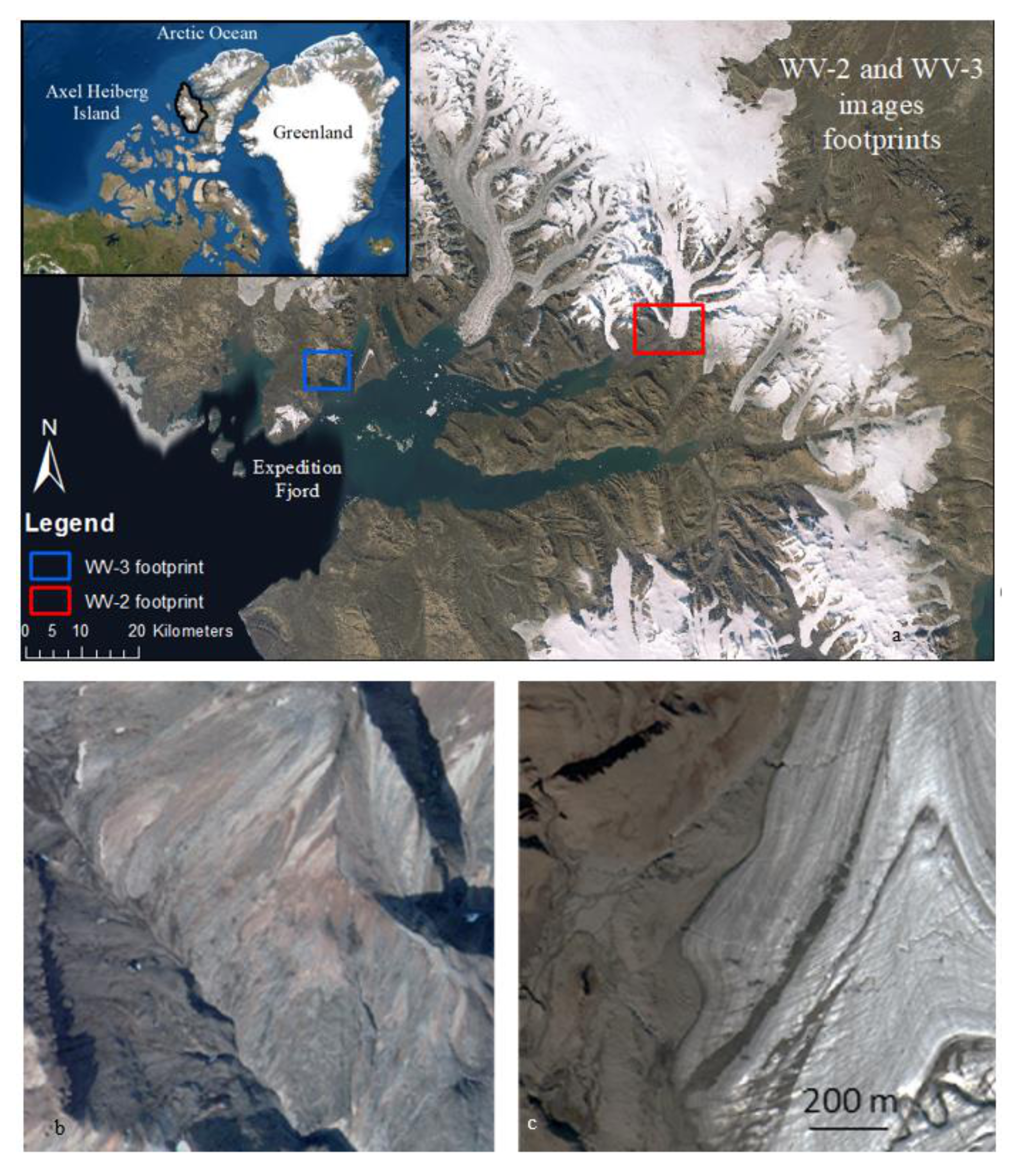
| WorldView imagery | 2 m | Axel Heiberg Island (Canada) |
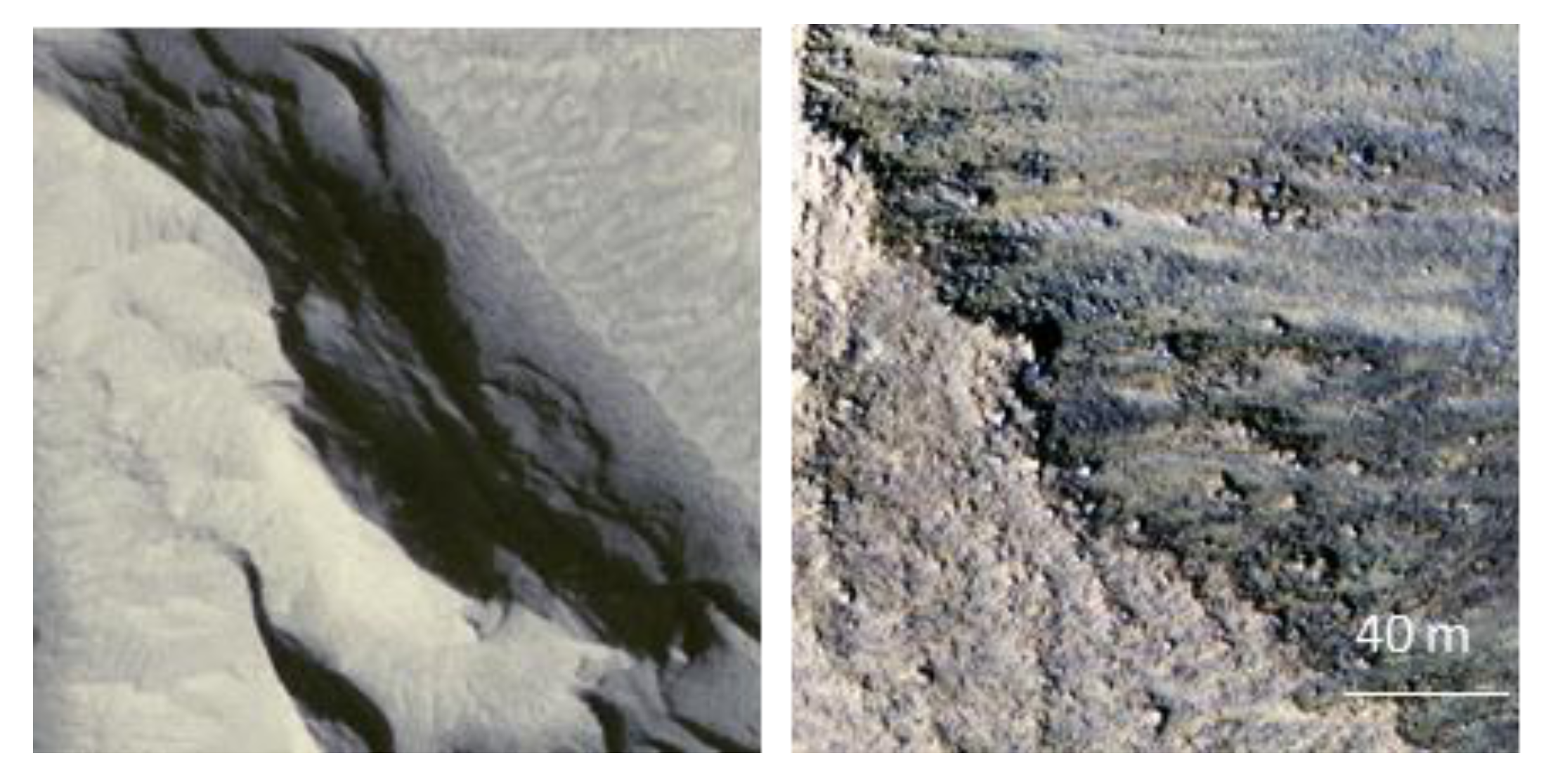
| HiRISE imagery | 25–50 cm | Mars |
| Averaged PSNR in dB for 150 and 300 Epochs | Averaged PSNR in dB for 2400 and 4800 Epochs | Enhancement % | |
|---|---|---|---|
| Mars theme | 32.95 | 38.13 | 15.72% |
| Outcrops theme | 35.69 | 36.68 | 2.77% |
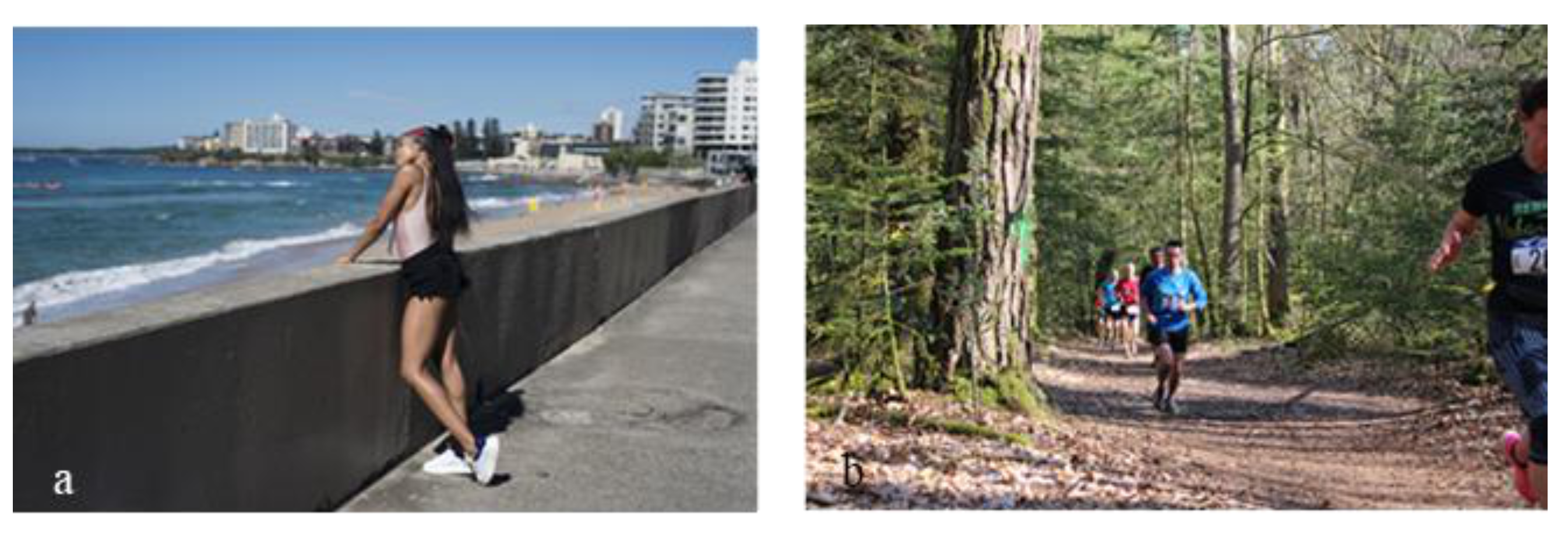
| Daily life theme | 30.92 | 31.63 | 2.29% |
| Crops theme | 30.47 | 30.59 | 0.39% |
| Urban theme | 29.16 | 30.09 | 0.87% |
| Forest theme | 29.83 | 30.00 | 0.57% |
| Mixed theme | 30.91 | 33.03 | 6.86% |
Publisher’s Note: MDPI stays neutral with regard to jurisdictional claims in published maps and institutional affiliations. |
© 2021 by the authors. Licensee MDPI, Basel, Switzerland. This article is an open access article distributed under the terms and conditions of the Creative Commons Attribution (CC BY) license (https://creativecommons.org/licenses/by/4.0/).
Share and Cite
Clabaut, É.; Lemelin, M.; Germain, M.; Bouroubi, Y.; St-Pierre, T. Model Specialization for the Use of ESRGAN on Satellite and Airborne Imagery. Remote Sens. 2021, 13, 4044. https://doi.org/10.3390/rs13204044
Clabaut É, Lemelin M, Germain M, Bouroubi Y, St-Pierre T. Model Specialization for the Use of ESRGAN on Satellite and Airborne Imagery. Remote Sensing. 2021; 13(20):4044. https://doi.org/10.3390/rs13204044
Chicago/Turabian StyleClabaut, Étienne, Myriam Lemelin, Mickaël Germain, Yacine Bouroubi, and Tony St-Pierre. 2021. "Model Specialization for the Use of ESRGAN on Satellite and Airborne Imagery" Remote Sensing 13, no. 20: 4044. https://doi.org/10.3390/rs13204044
APA StyleClabaut, É., Lemelin, M., Germain, M., Bouroubi, Y., & St-Pierre, T. (2021). Model Specialization for the Use of ESRGAN on Satellite and Airborne Imagery. Remote Sensing, 13(20), 4044. https://doi.org/10.3390/rs13204044