Abstract
Weeds are one of the main factors affecting the yield and quality of agricultural products. Accurate evaluation of weed density is of great significance for field management, especially precision weeding. In this paper, a weed density calculating and mapping method in the field is proposed. An unmanned aerial vehicle (UAV) was used to capture field images. The excess green minus excess red index, combined with the minimum error threshold segmentation method, was used to segment green plants and bare land. A modified U-net was used to segment crops from images. After removing the bare land and crops from the field, images of weeds were obtained. The weed density was evaluated by the ratio of weed area to total area on the segmented image. The accuracy of the green plant segmentation was 93.5%. In terms of crop segmentation, the intersection over union (IoU) was 93.40%, and the segmentation time of a single image was 35.90 ms. Finally, the determination coefficient of the UAV evaluated weed density and the manually observed weed density was 0.94, and the root mean square error was 0.03. With the proposed method, the weed density of a field can be effectively evaluated from UAV images, hence providing critical information for precision weeding.
1. Introduction
Weeds are one of the main causes of crop yield reduction and quality decline [1,2]. They compete with crops in the field for water, nutrients, and sunlight. This has led to about a 34% reduction in crop yield worldwide [3]. Currently, spraying herbicides is the most common way of weeding around the world [4]. Weeding is usually done by evenly spraying herbicides over the field, regardless of the density of weeds, which leads to over-spraying in areas absent of weeds. This approach to weeding causes herbicide waste and pollution of the agricultural ecological environment.
This method of weeding does not spray herbicides according to the presence or absence of weeds in an area [5]. Spraying in areas absent of weeds not only wastes herbicides but also pollutes the agricultural ecological environment. To solve these problems, the site-specific weed management (SSWM) method was proposed [6]. The main idea of SSWM is to weed according to the density or species of weeds. SSWM can not only effectively save herbicide, but also reduce environmental pollution caused by weeding. Weed density mapping plays a critical role in SSWM. Precise identification of weeds in the field and making weed density maps benefit weed management, while inaccurate weed maps may cause SSWM to fail or even cause crop damage [4].
In recent years, researchers have studied many methods of mapping weed density by machine vision and digital image processing [7,8]. Castillejo et al. used a multi-spectral QuickBird satellite to map the weed density in a winter wheat field [9]. However, the resolution of satellite images is relatively low and small groups of weeds cannot be detected by satellites effectively [10]. Therefore, the accuracy of a satellite-based weed density map is limited. There are also some researchers mapping weed density using sensors installed on an agricultural vehicle platform, mainly tractors [8,11,12,13]. In this method, sensors such as lidars, multispectral cameras, and hyperspectral cameras are installed close to the ground. These devices can obtain high-resolution images. However, it is time consuming to collect images from large-scale fields with this method. Moreover, the amount of data is large, which leads to a large amount of calculation in processing the images, so it is difficult to get a panoramic weed map of the field [7].
Unmanned aerial vehicles (UAVs) have shown great prospects in agricultural remote sensing [14,15,16,17]. UAVs can be equipped with various sensors, such as red, green, blue (RGB) cameras, hyperspectral cameras, multispectral cameras, three dimensional cameras, and lidars, which can be used to collect agricultural information [18,19,20,21,22]. Tamouridou et al. [23] used a multispectral camera (green–red–near-infrared) mounted on a fixed-wing UAV to map Silybum marianum weed patches, with an overall accuracy of 87.04%. Stroppiana et al. [24] used a multispectral camera on a quadcopter to segment weeds by an unsupervised clustering algorithm. The overall accuracy was 96.5%. Alexandridis et al. [25] used a multispectral camera (green–red–NIR) on a fixed-wing UAV to detect weeds, resulting in an overall accuracy of 96%. However, the spectral cameras, 3D cameras, and lidars mentioned above are expensive. They are usually used in the case of large land- and time-scales [6]. An RGB camera is a more cost-effective sensor, as it is smaller and lighter than other kinds of sensors. Hence, UAVs are equipped with RGB cameras in most cases.
UAVs implemented with RGB cameras were applied for weed mapping by some researchers. Gao et al. [7] developed a semi-automatic object-based image analysis (OBIA) algorithm with random forests (RF) combined with feature selection techniques to classify soil, weeds, and maize on UAV images. The results showed that the coefficient of determination was 0.895 and the root mean square error was 0.026. Gašparović et al. [26] proposed an automatic method for weed mapping in oat fields based on UAV imagery and a K-means algorithm, resulting in an overall accuracy of 89.0%. These methods segment weeds with manually defined features and classifiers. They have obtained relatively good results in detecting weeds, but the mapping of weed density remains a challenge. This is because these methods must have robust manually defined features, but these features are hard to find due to the similarity of weeds and crops in images, especially in the early stage of growth [27].
Convolutional neural networks can obtain abstract image features. They can effectively extract features that are difficult to define manually. Due to the application of convolutional neural networks (CNNs), image processing technology has made great progress [28,29,30]. CNNs have been widely applied in agriculture, especially in agricultural image processing [31,32,33,34]. Some researchers have applied CNNs to segmenting weeds on images. Huang et al. [35] proposed a weed segmentation method based on a fully convolutional network (FCN), resulting in a 0.883 segment accuracy. However, the weeds and crops in this experiment grew on different plots. The performance of this network on crops and weeds growing in a symbiotic environment has not been tested. At the same time, FCNs have insufficient accuracy in detail segmentation [36]. Therefore, it is necessary to study a UAV RGB image segmentation algorithm in the symbiotic environment of crops and weeds to map the weed density.
In this study, a marigold field was taken as the research object. A field weed density mapping method based on deep learning and UAV imaging was proposed. The two main objectives of this paper are
- To develop a semantic weed segmentation algorithm based on deep learning;
- To design a weed density calculation and mapping method based on segmented UAV images.
2. Materials and Methods
2.1. Marigold Field Image Acquisition and Sample Preparation
The research site was an experimental marigold field. The marigolds were in the seedling stage. The weed density in the field was various. The site is in the Shangzhuang experimental station of the China Agricultural University, Beijing, China (116.191794°E, 40.144091°N), shown in Figure 1. The crops were sown on 25 August 2020. No weeding was carried out after planting. The field was naturally infested by weeds including green bristlegrass, milkweed, and sedge. The images used in this research were taken from 10:00 to 12:00 on 26 September 2020.
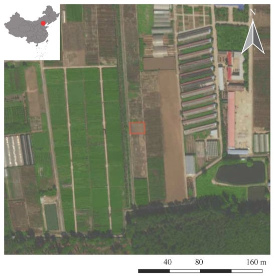
Figure 1.
Experiment location.
The images were obtained by a UAV (DJI, MAVIC 2, Shown in Figure 2). The ground station software was a DJI GO PRO (2.0.10). The flight height was 20 m. The flight speed was 14 m/s. The angle between the camera and the ground was 90. The original images were at a resolution of 5472 × 3648. The front overlap ratio was more than 80% and the side overlap ratio was more than 60%. The ground station software interface and further mission details are shown in Figure 3.

Figure 2.
Mavic 2 Pro.
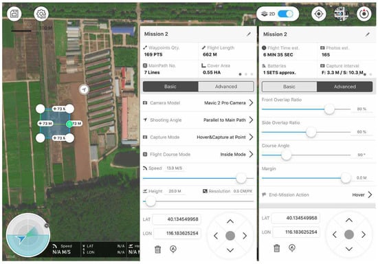
Figure 3.
Interface of DJI GO PRO and mission details.
The aerial photos were mosaicked by Agisoft PhotoScan Professional Edition 1.1.5 (Agisoft LLC, St. Petersburg, Russia). After mosaicking, a 12,750 × 12,750 image was obtained and the spatial resolution of this image was 5 mm/pixel. The mosaicked image is shown in Figure 4.
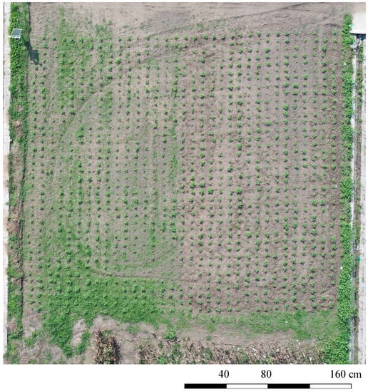
Figure 4.
The original mosaicked image.
The original mosaicked image was too large to directly use in the training of deep learning neural networks, so a series of 256 × 256 pixels images were randomly cut out from the mosaicked image (shown in Figure 5a). These images were used to train the networks. Some of these images are shown in Figure 5b. The sample images were manually annotated using Adobe Photoshop CC 2019. The pixel value at the target domain of the marigolds was set as 1, and the soil and weed pixel value was 0. A total of 100 images were obtained. Among these images, 80 images were used for network training, 10 images were used for validation, and 10 images were used for network testing [17].
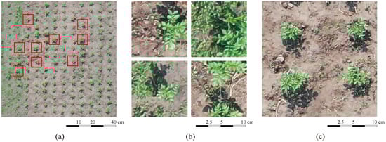
Figure 5.
Training and testing samples: (a) images cut from the mosaicked image; (b) images for network training; (c) images for weed density accuracy testing.
At the same time, 50 images with a size of pixels were randomly cut from the mosaicked image. These images were used to test the accuracy of weed density calculated by the algorithm. Some of these images are shown in Figure 5c. These images were labeled weed density by expert manual inspection, and the inspection results were seen as the ground truth.
2.2. Process of Weed Density Evaluation from UAV Images
There are four main procedures to evaluate weed density by UAV images: (1) UAV image mosaic; (2) green plant segmentation; (3) crop segmentation; (4) weed coverage calculation. First of all, the UAV images were stitched into a complete image with the help of software to obtain the original field map. Then, the green plant parts in the image were segmented out by the excess green (ExG) index and threshold segmentation. Then, with the help of a neural network, the crops in the image were segmented out. Weed covered parts were obtained by removing the crop part from the green plant parts. Finally, the weed coverage rate was calculated. The weed density map of the whole field was obtained. The overall flowchart of evaluating weed density by UAV is shown in Figure 6.
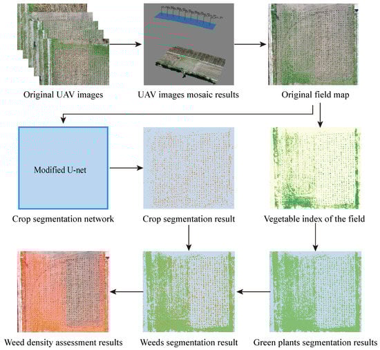
Figure 6.
Flowchart of weed density evaluation and mapping by unmanned aerial vehicle (UAV).
2.3. Green Plant Segmentation Method
In this study, the research team randomly selected 4 images from the training images, and randomly selected 300 pixels from these 4 images. We manually labeled whether these pixels were bare land pixels (value set as 0) or green plants (value set as 1). In these pixels, 200 pixels were used to calculate the segmentation threshold, and 100 pixels were used to test the accuracy of segmentation. The sample points and labels are shown in Figure 7.

Figure 7.
Sample points for green plant segmentation.
Green plants and bare land are different in color, so it is easy to segment green plants by color. The vegetation indexes are a kind of color feature. They can magnify the differences between green plants and others. Excess green minus excess red (ExG_EXR) is a commonly used vegetation index. It was designed to segment green plants from bare land [37]. The calculation method is shown in Equations (1)–(3).
where r is the R-channel value in the RGB color space divided by 255, g is the G-channel value in the RGB color space divided by 255, and b is the B-channel value in the RGB color space divided by 255.
In this paper, the minimum error segmentation method is used to segment the green plants on the excess green minus excess red index. The diagram of this method is shown in Figure 8. The minimum error segmentation method is a segmentation method based on the normal distribution. It is assumed that the foreground (the normal distribution curve of the foreground is shown in Figure 8a) and background (the normal distribution curve of the background is shown in Figure 8b) in the image obey a normal distribution. According to the characteristics of the two normal distributions, the intersection point of the two normal distribution curves (shown in Figure 8o) is used as the segmentation threshold. This point is the threshold with the smallest segmentation error in theory. The calculation method of point (o) is shown in Equations (4) and (5). Since the images described in this paper were obtained under natural conditions, they all obey a normal distribution. Therefore, this method was used to find the segmentation threshold.
where and are the mean values of two kinds of sample pixels, and and are the root mean square errors of two kinds of sample pixels.
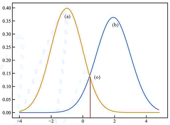
Figure 8.
Diagram of minimum error method: (a) normal distribution curve of foreground; (b) normal distribution curve of background; (o) intersection point of the two normal distribution curves.
2.4. Crop Segmentation Network Structure
U-net is a very common semantic segmentation network [17,38]. The shape of the network is like a “U” (shown in Figure 9a) [39]. At first, it was invented to segment biological images. U-nets have also achieved good results in other industries. There are two main reasons why they work so well. Firstly, this model can extract global features related to local information through convolution layers. Secondly, U-net can perform well trained by a very small number of training samples [17]. However, due to the complexity of the classical U-net and the large consumption of computing resources, the speed of it was slow. Therefore, a modified U-net was proposed by simplifying the U-net.
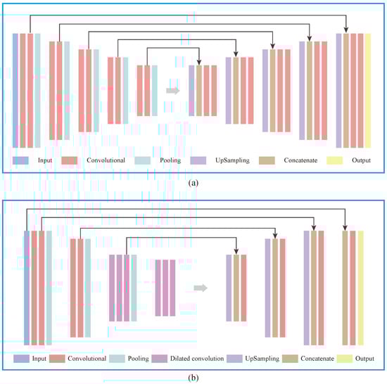
Figure 9.
(a) Structure of U-net; (b) structure of modified U-net.
Dilation convolution can be used to replace the pooling layer. Dilation convolution can maintain high resolution, at the same ensuring the receptive field [40]. However, dilated convolution has an inherent problem: the information in the hole is missed. Hybrid division convolution (HDC) was proposed to solve the problem of detail information loss in dilated convolution [41]. In a series of division convolution layers, a series of related dilation rates is used to supplement the other parts of the hole [28]. In the HDC framework, a sawtooth wave-like heuristic is used to assign a dilation rate. The “rising edge” of the wave that has an increasing dilation rate formed by a series of layers is grouped, and the next group repeats the same pattern. In addition, the dilation rate within a group should not have a common factor relationship (like R = 1, 2, 3, etc.) [42]. In this study, HDC was used to modify the backbone network of U-net. As shown in Figure 9b, the last two convolution blocks of the VGG16 network were replaced by HDC blocks. The HDC blocks were composed of a stacked cascade mode, and the dilation rates R were 1, 2, and 5. Two HDC blocks were connected by a pooling layer and placed at the end of the backbone.
Another important part of U-net besides the backbone is the decoder. The decoder is used to recover high-level semantic features and spatial information. The decoder module in U-net is mainly composed of upsampling and convolution layers. The decoder part of the U-net consists of four blocks, each block consisting of an upsampling layer, a connecting layer, and two convolution layers. The upsampling layer is used for upsampling, and the connecting layer is used to connect the feature maps obtained from the encoder blocks. The convolution layer is used to generate features for semantic segmentation. In this study, the complexity of images was low, but the required accuracy of segmentation in details was high. Therefore, two convolution layers of each block were reduced to one and the input layer was connected with the last decoder block. This reduces the complexity of the network and increases the ability of the network to segment the details.

Table 1.
Structure of the modified U-net.
2.5. Modified U-Net Training
The hardware environment was an Intel Core i7-9700 K CPU, 16 GB memory, and an NVIDIA GeForce RTX 2080 Super. The software environment was Windows 10, CUDA 10.1, Python 3.6, Tensorflow 2.3.
In this study, the segmentation of crops is a binary classification problem, in which it is considered whether the pixel is a crop pixel or not. Similar to other binary classification networks, the cross-entropy was used as the loss function, which was calculated as Equation (6). During parameter training, the neural networks were trained by a gradient descent method. The “Adam” optimizer was used to optimize the network. The initial learning rate was 0.0001 and the learning rate attenuation coefficient was 0.001. When the training iteration times reached 100, the training stopped and saved the model.
where p is the true value, q is the predicted value, and k is the pixel number.
Data augmentation can increase the richness of sample images and it can also improve the adaptability of neural networks. There are many methods of data augmentation, such as rotation, mirror image, increasing noise, and so on [17]. The most common data augmentation method is using rotation and mirroring to augment images to about 5 times. Therefore, we adopted rotation ±5, ±10 and mirroring to augment the samples. After data augmentation, the number of samples increased to 500. The training set increased to 400 images. The validation set and the testing set increased to 50 images. Ten images were randomly selected from the training set to form a batch.
2.6. Crop Segment Network Performance Evaluation
In this study, 5 quantitative criteria were used to evaluate the segmentation network. The overall pixel accuracy (Acc), precision (Pr), recall (Re), and Intersection over Union (IoU) were used to assess and compare the segmentation performance (Equations (7)–(10)). The Acc, Pr, Re, Fm, and IoU were averaged over all images in the testing dataset. We also compared the segmentation time. The segment time (ST) is the time needed to segment a single image. It was recorded by the program during segmenting the images.
where is true positive; is true negative; is false positive; is false negative.
2.7. Weed Density Calculating and Mapping
The original image was too large to process, especially for deep learning networks. In order to evaluate the weed density and make the weed density map, the field image obtained by UAV was divided into many sub-images with the size of pixels. These sub-images were input into the green plant segmentation algorithm and the modified U-net. The green plant parts and the crop parts in the image were obtained. Weed covered parts were obtained by removing the crop parts from the green plant parts. The value of pixels at the weed-covered parts was set as 1, and the pixel value at the other parts was set as 0. After median filtering with the size of 1000 × 1000, weed density maps were obtained.
In the field weed degree investigation, the ratio of weed area to total area is an important index, and its calculation method is shown in Equation (11). In order to test the accuracy of the proposed weed density evaluated by the algorithm, the of the 50 images with a size of pixels used to test the accuracy of weed density were calculated. Then the relationship between the calculated from the UAV image (predicted ) and the by expert visual observation (observed ) was evaluated by regression analysis. Two criteria were calculated and considered. The coefficient of determination () was computed by Equation (12). The root mean square error () was determined with Equation (13).
where is the ratio of weed area, is the area of weeds and is the area of the whole field.
where, and are, respectively, the i-th observed and predicted from N total data.
3. Results
3.1. Green Plant Segmentation Results
The frequency distribution histogram and the fitting normal distribution curve are shown in Figure 10a. As can be seen from the figure, the two types of samples showed normal distribution on the excess green minus excess red index. At the same time, their normal distribution centers were not coincident. Therefore, it was feasible to use the minimum error method to calculate the segmentation threshold. It can be seen from the graph that the minimum segmentation error can be obtained at the intersection of normal fitting curves. However, there were still some errors, because the two curves overlap. The threshold value of segmentation calculated by the minimum error segmentation method was 0.13. Using 0.13 as the threshold to segment the test set, the segmentation accuracy was 93.5%. The segmentation result of the original image using this threshold is shown in Figure 10b.
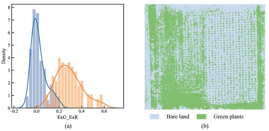
Figure 10.
(a) Frequency distribution histogram and fitting normal distribution curve; (b) segment result.
3.2. Training Process of the Modified U-Net
Figure 11 shows the accuracy and loss of the model in the training set and test set as the number of iterations increases. From this figure, it can be seen that, during the training, the accuracy of the training set and verification set was stable after rising, and the loss value tended to be stable after decreasing. In other words, the loss of both sets was decreasing, and the accuracy was gradually improved. After approximately 20 iterations of training, the accuracy and loss value tended to be stable. At the same time, there was no significant gap between the accuracy and loss value between the training set and the verification set, so there was no overfitting. After 100 iterations, the loss value and accuracy converged. This showed that the model achieved a good training effect. After training, the mean pixel classification accuracy of the model was 98.84%, the IoU was 93.40%, precision was 93.40%, recall rate was 80.85%, and the average segmentation time of a single image was 40.90 ms.
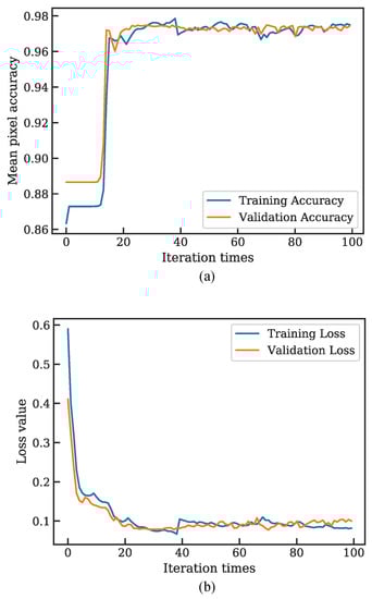
Figure 11.
Accuracy and loss value changes of the training and validation sets during training: (a) training and validation accuracy; (b) training and validation loss.
3.3. Comparison of Modified U-Net with State-of-the-Art Methods
The proposed algorithm was compared with state-of-the-art methods such as Otsu threshold segmentation, color texture, and shape + SVM, FCN, Segnet, and U-Net [35,37,39,43,44]. The original image, label, and segmentation results of the modified U-net and state-of-the-art image segmentation methods are shown in Figure 12. The evaluation results are shown in Table 2.

Figure 12.
Original image, label, and segmentation results of different algorithms. (a) Original image; (b) label; (c) proposed algorithm; (d) U-net; (e) SegNet; (f) fully convolutional network (FCN); (g) color texture and shape + SVM; (h) threshold.
Table 2.
Evaluation of segmentation effects of different segmentation algorithms.
As can be seen in Table 2, the performance of threshold segmentation was the worst among all segmentation methods. The IoU, accuracy, precision, recall, and segment time on the test set were 71.49%, 85.97%, 64.25%, 92.02%, and 0.24 ms, respectively. By observing the original image, it can be found that there were mainly bare land, weeds, and crops in the images. In the early stage of crop growth, the color of crops is close to that of weeds. When the Otsu threshold is used for segmentation of the G–R index, it is easy to divide bare land into one category, and weeds and crops into another category. As can be seen from the segmented image by this method, many weeds were also classified as crops. As a result, IoU, accuracy, and accuracy based on threshold segmentation were not high, but the recall rate was relatively high. Although the threshold segmentation method takes less time, it is not suitable for the construction of a weed map due to the poor segmentation effect.
Compared with the Otsu threshold segmentation, the color texture and shape + SVM segmentation method had a better segmentation performance. The IoU, accuracy, precision, recall, and segment time on the test set were 75.02%, 89.80%, 70.96%, 84.31%, and 1.74 ms, respectively. There are some differences in the texture and shape between weed leaves and crop leaves, so this method achieved better results by introducing these features. At the same time, the SVM classifier can achieve a better classification effect than threshold segmentation in the multi-feature fusion classification task. This algorithm is more complex and the time consumed for a single image by this method is longer due to more features and more complex classification methods. The classification performance of this method was still poor, which cannot meet the needs of weed map construction.
The FCN, Segnet, and U-net are deep semantic segmentation neural networks based on convolutional neural networks. The IoU, accuracy, precision, recall, and segment time of FCN were 68.78%, 90.89%, 54.61%, 77.15%, 49.79 ms, respectively. It can be seen from Figure 12 that there was significant noise in the segmentation results for the FCN. At the same time, the edge of segmentation was very rough. This was because the FCN directly uses the feature layer extracted from the neural network for classification. There was no convolution in the decoder stage, so the ability for edge detail and noise processing was poor. The IoU, accuracy, precision, recall, and segment time of Segnet were 84.43%, 96.69%, 74.64%, 72.21%, 41.43 ms, respectively. It can be seen from Figure 12 that the noise was suppressed well compared with the segmentation results of the FCN. At the same time, the edges were smoother. This is because the upsampling layers and the convolution layer were used to fuse features. Although the Segnet segmentation edge was smoother, the segment accuracy was still poor. The IoU, accuracy, precision, recall, and segment time for U-net were 92.33%, 98.62%, 82.43%, 80.55%, 44.24 ms, respectively. In the U-net, the results of each upsampling were fused with the feature layers of the corresponding convolution layer, so the performance of the U-net for detail processing was better. However, due to the complexity of the neural network structure, the training of the neural network was difficult and the segmentation time was long.
The IoU, accuracy, precision, recall, and segment time of the proposed modified U-net were 93.40%, 98.84%, 84.29%, 80.85%, 40.90 ms, respectively. HDC layers ensure the accuracy of detail extraction and the size of the perceptual field. Compared with the convolution and pooling block, it not only ensures the performance of feature extraction but also simplifies the network. At the same time, because the input layer was input before the output convolution layer as a feature map, this increased the detail features, and enhanced the ability of detail segmentation of the network. Therefore, the proposed modified U-net consumed less time and achieved a slightly better segmentation effect than U-net. The result of crop segmentation of the original image by the modified U-net is shown in Figure 13.

Figure 13.
Crop segmentation result.
3.4. Weed Mapping and Accuracy Evaluation Results
The original map and weed density maps are shown in Figure 14, and the regression analysis results of the UAV evaluation result and the manual evaluation result are shown in Figure 15. Regression analysis showed that the relationship between the predicted weed density and the manually observed weed density was y = 0.87x − 0.00. The coefficient of determination was 0.94, and the root mean square error () was 0.03. This indicated that the correlation between the two was good. It was effective to evaluate weed density by UAV. The slope of the relationship was 0.87, and the intercept was −0.00. This showed that the evaluation of weed density by UAV was slightly higher than the result of manual evaluation. By observing the original image and the segmentation result map, it can be found that the bare land segmentation was more accurate, and the error mainly comes from the segmentation of crops. Some weeds were wrongly segmented into crops, and some crop edges were wrongly segmented into weeds. Therefore, the weed density evaluated by UAV was slightly higher than that evaluated by manual observation. In the future, a more accurate crop segmentation algorithm can be studied to improve evaluation accuracy.
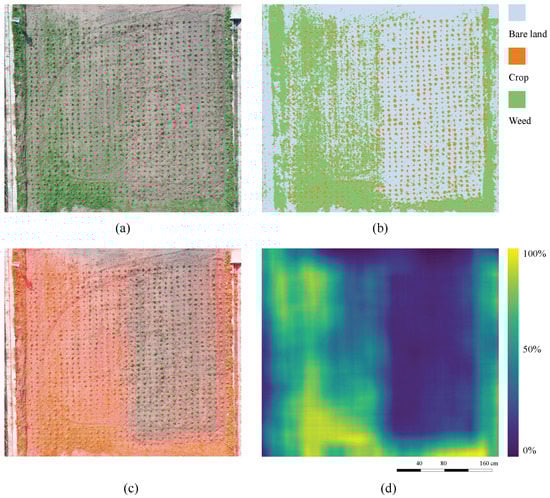
Figure 14.
Original map and weed density maps: (a) original map; (b) result map of bare land, weed, and crop segmentation; (c) mixed map of weed density; (d) heat map of weed density.
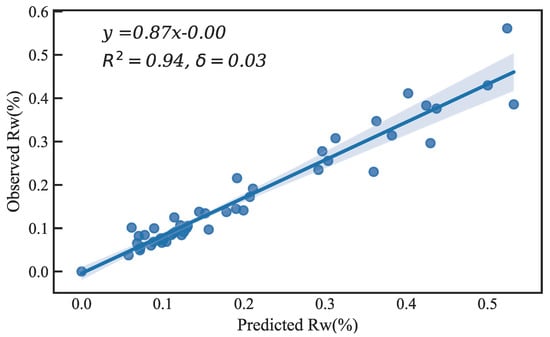
Figure 15.
Regression analysis results of UAV evaluation and manual evaluation.
4. Discussion
In this paper, UAV images were used to assess and map the weed density in the field. We proposed a modified U-net based on the traditional U-net. This neural network was effective in segmenting the crops in the images. Combining the neural-network-based crop segmentation and the threshold-based bare land and green plant segmentation methods, a weed segmentation algorithm that successfully segmented weeds on the image, and calculated and mapped the weed density was constructed. The coefficient of determination () between the algorithm-predicted result and the observed result was 0.94, and the root mean square error () was 0.03. An image feature and SVM-based and threshold-based weed detection method were also used to measure weed density in the experimental fields of this study [7,26,37,43]. These methods were used to segment weeds directly from the images, instead of segmenting green plants and crops in two steps. The results showed that the () and () of the image feature and SVM-based method measured were 0.87 and 0.05, respectively. The () and () of the threshold-based method measured were 0.74 and 0.10, respectively. These results show that the proposed algorithm can assess weed density more accurately in the field.
The weed density assessment method described in this paper mainly consists of green plant segmentation and crop weed segmentation. We did not use a multi-class segmentation neural network to segment the image into bare land, weeds, and crops directly. This was because the semantic segmentation neural network requires a large number of manually labeled images, pixel by pixel, as training samples. Weeds are very small on UAV images. It is difficult to segment weed images pixel by pixel with the human eye on the UAV images. Both weeds and crops in this study were green vegetation. There was a large difference in color between the green vegetation and bare land, and color-based threshold segmentation can be used to segment the green plants. Crops are larger compared to weeds and are relatively easy to label manually. Therefore, a method of training neural networks using manually labeled crops is feasible. The research method described in this paper takes full consideration of the image features and the advantages of the two image segmentation methods and provides an effective combination of the two methods, which in turn successfully calculates the weed density from UAV images.
This paper proposed a modified U-net based on the traditional U-net. The image segmentation task in this paper is a binary classification task, involving crop and non-crop classification. At the same time, the complexity of the image was also low. Therefore, the feature extraction part (baseline) of the neural network was simplified. This kind of simplification reduced the feature extraction ability of the neural network, but the requirement of this ability in this paper was low. This simplification improved the speed of the neural network. The segmentation accuracy of this network was slightly higher than that of U-net, but its complexity was lower than that of U-net, and its running speed was higher. The neural network simplification was effective. The performance of this network in more complex image classification problems may not be as good as others. However, the performance in this study is better than other networks.
The training data for the neural network proposed in this paper were only collected in a marigold field and the weed species was mainly green bristlegrass. This crop segmentation network may not work well in other fields or fields with other weed species. Therefore, in the future, we will collect more diverse data to enhance the robustness and adaptability of the segmentation network. This will allow it to be used in a wider range of applications.
The weed density assessment methods studied in this article are not very meaningful when used alone. However, they were developed to provide reference information for ground precision weeding equipment. The weed control equipment will selectively allow precision weeding based on weed density maps. Ground weeding equipment operates in areas of high weed density according to the weed map. It saves costs and reduces pollution by herbicides. The scope of our research is relatively small, and it is possible to extend the scope by using a UAV with a large flight area. At the same time, this kind of high precision result obtained on a small scale can be used as a ground truth to develop precision weed assessment algorithms for large scope areas, such as satellite remote sensing.
5. Conclusions
In this paper, a method to evaluate and map weed density by UAV images was proposed. Combining neural-network-based crop segmentation and threshold-based bare land and green plant segmentation methods, a weed segmentation algorithm that successfully calculated and mapped weed density was constructed. Through the analysis of the experimental results, it was found that
- (1)
- The combination of excess green minus excess red index and the minimum error method could be used to segment bare land and green plants. The segmentation accuracy could reach 93.5%.
- (2)
- The proposed modified U-net can effectively segment weeds and crop images. The IoU of segmentation was 93.40%, and the segmentation time of a single image was 40.90 ms;
- (3)
- Weed density in the field can be effectively evaluated by UAV images. The coefficient of determination was 0.94, and the root mean square error () was 0.03.
- (4)
- The results show that weed density could be calculated and mapped by UAV and image segmentation. The results for this method are reasonable and provide effective information for precise weed management and precision weeding.
Author Contributions
Writing—original draft preparation, K.Z.; methodology, C.Z.; writing—review and editing, X.C., F.Z., and H.Z.; project administration, C.Z.; funding acquisition, C.Z. All authors have read and agreed to the published version of the manuscript.
Funding
This research was funded by the National Key Research and Development Project of China (2019YFB1312303).
Institutional Review Board Statement
Not applicable.
Informed Consent Statement
Informed consent was obtained from all subjects involved in the study.
Data Availability Statement
The data presented in this study are available on request from the corresponding author. The data are not publicly available due to [A more in-depth study of the relevant data is underway and some of the results are not yet publicly available.].
Conflicts of Interest
The authors declare no conflict of interest.
References
- Wang, A.; Zhang, W.; Wei, X. A review on weed detection using ground-based machine vision and image processing techniques. Comput. Electron. Agric. 2019, 158, 226–240. [Google Scholar] [CrossRef]
- Hamuda, E.; Glavin, M.; Jones, E. A survey of image processing techniques for plant extraction and segmentation in the field. Comput. Electron. Agric. 2016, 125, 184–199. [Google Scholar] [CrossRef]
- Oerke, E.-C. Crop losses to pests. J. Agric. Sci. 2006, 144, 31–43. [Google Scholar] [CrossRef]
- Christensen, S.; Søgaard, H.T.; Kudsk, P.; Nørremark, M.; Lund, I.; Nadimi, E.S.; Jørgensen, R. Site-specific weed control technologies. Weed Res. 2009, 49, 233–241. [Google Scholar] [CrossRef]
- López-Granados, F.; Torres-Sánchez, J.; Serrano-Pérez, A.; de Castro, A.I.; Mesas-Carrascosa, F.J.; Pena, J.M. Early season weed mapping in sunflower using UAV technology: Variability of herbicide treatment maps against weed thresholds. Precis. Agric. 2016, 17, 183–199. [Google Scholar] [CrossRef]
- López-Granados, F. Weed detection for site-specific weed management: Mapping and real-time approaches. Weed Res. 2011, 51, 1–11. [Google Scholar] [CrossRef]
- Gao, J.; Liao, W.; Nuyttens, D.; Lootens, P.; Vangeyte, J.; Pižurica, A.; He, Y.; Pieters, J.G. Fusion of pixel and object-based features for weed mapping using unmanned aerial vehicle imagery. Int. J. Appl. Earth Obs. Geoinf. 2018, 67, 43–53. [Google Scholar] [CrossRef]
- Zhou, H.; Zhang, J.; Ge, L.; Yu, X.; Wang, Y.; Zhang, C. Research on volume prediction of single tree canopy based on three-dimensional (3D) LiDAR and clustering segmentation. Int. J. Remote Sens. 2020, 42, 738–755. [Google Scholar] [CrossRef]
- Castillejo-González, I.L.; Peña-Barragán, J.M.; Jurado-Expósito, M.; Mesas-Carrascosa, F.J.; López-Granados, F. Evaluation of pixel-and object-based approaches for mapping wild oat (Avena sterilis) weed patches in wheat fields using QuickBird imagery for site-specific management. Eur. J. Agron. 2014, 59, 57–66. [Google Scholar] [CrossRef]
- de Castro, A.I.; López-Granados, F.; Jurado-Expósito, M. Broad-scale cruciferous weed patch classification in winter wheat using QuickBird imagery for in-season site-specific control. Precis. Agric. 2013, 14, 392–413. [Google Scholar] [CrossRef]
- Lottes, P.; Hörferlin, M.; Sander, S.; Stachniss, C. Effective vision-based classification for separating sugar beets and weeds for precision farming. J. Field Robot. 2017, 34, 1160–1178. [Google Scholar] [CrossRef]
- Rehman, T.U.; Zaman, Q.U.; Chang, Y.K.; Schumann, A.W.; Corscadden, K.W.; Esau, T.J. Optimising the parameters influencing performance and weed (goldenrod) identification accuracy of colour co-occurrence matrices. Biosyst. Eng. 2018, 170, 85–95. [Google Scholar] [CrossRef]
- Tao, T.; Wu, S.; Li, L.; Li, J.; Bao, S.; Wei, X. Design and experiments of weeding teleoperated robot spectral sensor for winter rape and weed identification. Adv. Mech. Eng. 2018, 10, 1687814018776741. [Google Scholar] [CrossRef]
- Du, M.; Noguchi, N. Monitoring of wheat growth status and mapping of wheat yield’s within-field spatial variations using color images acquired from UAV-camera system. Remote Sens. 2017, 9, 289. [Google Scholar] [CrossRef]
- Nevavuori, P.; Narra, N.; Lipping, T. Crop yield prediction with deep convolutional neural networks. Comput. Electron. Agric. 2019, 163, 104859. [Google Scholar] [CrossRef]
- Xu, W.; Yang, W.; Chen, S.; Wu, C.; Chen, P.; Lan, Y. Establishing a model to predict the single boll weight of cotton in northern Xinjiang by using high resolution UAV remote sensing data. Comput. Electron. Agric. 2020, 179, 105762. [Google Scholar] [CrossRef]
- Zhou, D.; Li, M.; Li, Y.; Qi, J.; Liu, K.; Cong, X.; Tian, X. Detection of ground straw coverage under conservation tillage based on deep learning. Comput. Electron. Agric. 2020, 172, 105369. [Google Scholar] [CrossRef]
- Rasmussen, J.; Nielsen, J.; Garcia-Ruiz, F.; Christensen, S.; Streibig, J.C. Potential uses of small unmanned aircraft systems (UAS) in weed research. Weed Res. 2013, 53, 242–248. [Google Scholar] [CrossRef]
- Costa, L.; Nunes, L.; Ampatzidis, Y. A new visible band index (vNDVI) for estimating NDVI values on RGB images utilizing genetic algorithms. Comput. Electron. Agric. 2020, 172, 105334. [Google Scholar] [CrossRef]
- Liu, Y.; Liu, S.; Li, J.; Guo, X.; Wang, S.; Lu, J. Estimating biomass of winter oilseed rape using vegetation indices and texture metrics derived from UAV multispectral images. Comput. Electron. Agric. 2019, 166, 105026. [Google Scholar] [CrossRef]
- Cao, Y.; Li, G.L.; Luo, Y.K.; Pan, Q.; Zhang, S.Y. Monitoring of sugar beet growth indicators using wide-dynamic-range vegetation index (WDRVI) derived from UAV multispectral images. Comput. Electron. Agric. 2020, 171, 105331. [Google Scholar] [CrossRef]
- Ge, L.; Yang, Z.; Sun, Z.; Zhang, G.; Zhang, M.; Zhang, K.; Zhang, C.; Tan, Y.; Li, W. A method for broccoli seedling recognition in natural environment based on binocular stereo vision and gaussian mixture model. Sensors 2019, 19, 1132. [Google Scholar] [CrossRef] [PubMed]
- Tamouridou, A.; Alexandridis, T.; Pantazi, X.; Lagopodi, A.; Kashefi, J.; Moshou, D. Evaluation of UAV imagery for mapping Silybum marianum weed patches. Int. J. Remote Sens. 2017, 38, 2246–2259. [Google Scholar] [CrossRef]
- Stroppiana, D.; Villa, P.; Sona, G.; Ronchetti, G.; Candiani, G.; Pepe, M.; Busetto, L.; Migliazzi, M.; Boschetti, M. Early season weed mapping in rice crops using multi-spectral UAV data. Int. J. Remote Sens. 2018, 39, 5432–5452. [Google Scholar] [CrossRef]
- Alexandridis, T.K.; Tamouridou, A.A.; Pantazi, X.E.; Lagopodi, A.L.; Kashefi, J.; Ovakoglou, G.; Polychronos, V.; Moshou, D. Novelty detection classifiers in weed mapping: Silybum marianum detection on UAV multispectral images. Sensors 2017, 17, 2007. [Google Scholar] [CrossRef] [PubMed]
- Gasparovic, M.; Zrinjski, M.; Barkovi, C.D.; Radocaj, D. An automatic method for weed mapping in oat fields based on UAV imagery. Comput. Electron. Agric. 2020, 173, 105385. [Google Scholar] [CrossRef]
- Perez-Ortiz, M.; Manuel Pena, J.; Antonio Gutierrez, P.; Torres-Sanchez, J.; Hervas-Martinez, C.; Lopez-Granados, F. Selecting patterns and features for between- and within- crop-row weed mapping using UAV-imagery. Expert Syst. Appl. 2016, 47, 85–94. [Google Scholar] [CrossRef]
- He, K.; Zhang, X.; Ren, S.; Sun, J. Deep residual learning for image recognition. In Proceedings of the IEEE Conference on Computer Vision and Pattern Recognition, Las Vegas, NV, USA, 27–30 June 2016; pp. 770–778. [Google Scholar]
- Huang, H.; Deng, J.; Lan, Y.; Yang, A.; Deng, X.; Wen, S.; Zhang, H.; Zhang, Y. Accurate weed mapping and prescription map generation based on fully convolutional networks using UAV imagery. Sensors 2018, 18, 3299. [Google Scholar] [CrossRef]
- Huang, H.; Lan, Y.; Deng, J.; Yang, A.; Deng, X.; Zhang, L.; Wen, S. A semantic labeling approach for accurate weed mapping of high resolution UAV imagery. Sensors 2018, 18, 2113. [Google Scholar] [CrossRef]
- Kamilaris, A.; Prenafetaboldu, F.X. Deep learning in agriculture: A survey. Comput. Electron. Agric. 2018, 147, 70–90. [Google Scholar] [CrossRef]
- Chen, C.; Kung, H.; Hwang, F.J. Deep Learning Techniques for Agronomy Applications. Agronomy 2019, 9, 142. [Google Scholar] [CrossRef]
- Yang, Q.; Shi, L.; Han, J.; Zha, Y.; Zhu, P. Deep convolutional neural networks for rice grain yield estimation at the ripening stage using UAV-based remotely sensed images. Field Crops Res. 2019, 235, 142–153. [Google Scholar] [CrossRef]
- Fuentes, A.; Yoon, S.; Kim, S.C.; Park, D.S. A Robust Deep-Learning-Based Detector for Real-Time Tomato Plant Diseases and Pests Recognition. Sensors 2017, 17, 2022. [Google Scholar] [CrossRef] [PubMed]
- Huang, H.; Deng, J.; Lan, Y.; Yang, A.; Deng, X.; Zhang, L.; Gonzalez-Andujar, J.L. A fully convolutional network for weed mapping of unmanned aerial vehicle (UAV) imagery. PLoS ONE 2018, 13, e0196302. [Google Scholar] [CrossRef] [PubMed]
- Wang, H.; Gao, N.; Xiao, Y.; Tang, Y. Image feature extraction based on improved FCN for UUV side-scan sonar. Mar. Geophys. Res. 2020, 41, 1–17. [Google Scholar] [CrossRef]
- Meyer, G.E.; Neto, J.C. Verification of color vegetation indices for automated crop imaging applications. Comput. Electron. Agric. 2008, 63, 282–293. [Google Scholar] [CrossRef]
- Long, J.; Shelhamer, E.; Darrell, T. Fully convolutional networks for semantic segmentation. In Proceedings of the 2015 IEEE Conference on Computer Vision and Pattern Recognition (CVPR), Boston, MA, USA, 7–12 June 2015; pp. 3431–3440. [Google Scholar]
- Ronneberger, O.; Fischer, P.; Brox, T. U-Net: Convolutional Networks for Biomedical Image Segmentation. In Proceedings of the International Conference on Medical Image Computing and Computer-Assisted Intervention, Munich, Germany, 5–9 October 2015; pp. 234–241. [Google Scholar]
- Chen, L.C.; Papandreou, G.; Kokkinos, I.; Murphy, K.; Yuille, A.L. Deeplab: Semantic image segmentation with deep convolutional nets, atrous convolution, and fully connected crfs. IEEE Trans. Pattern Anal. Mach. Intell. 2017, 40, 834–848. [Google Scholar] [CrossRef]
- Wang, P.; Chen, P.; Yuan, Y.; Liu, D.; Huang, Z.; Hou, X.; Cottrell, G. Understanding convolution for semantic segmentation. In Proceedings of the 2018 IEEE Winter Conference on Applications of Computer Vision (WACV), Lake Tahoe, NV, USA, 12–15 March 2018; pp. 1451–1460. [Google Scholar]
- Tang, H.; Wang, B.; Chen, X. Deep learning techniques for automatic butterfly segmentation in ecological images. Comput. Electron. Agric. 2020, 178, 105739. [Google Scholar] [CrossRef]
- Zou, K.; Ge, L.; Zhang, C.; Yuan, T.; Li, W. Broccoli Seedling Segmentation Based on Support Vector Machine Combined With Color Texture Features. IEEE Access 2019, 7, 168565–168574. [Google Scholar] [CrossRef]
- Badrinarayanan, V.; Kendall, A.; Cipolla, R. Segnet: A deep convolutional encoder-decoder architecture for image segmentation. IEEE Trans. Pattern Anal. Mach. Intell. 2017, 39, 2481–2495. [Google Scholar] [CrossRef]


Publisher’s Note: MDPI stays neutral with regard to jurisdictional claims in published maps and institutional affiliations. |
© 2021 by the authors. Licensee MDPI, Basel, Switzerland. This article is an open access article distributed under the terms and conditions of the Creative Commons Attribution (CC BY) license (http://creativecommons.org/licenses/by/4.0/).