Abstract
Individual tree extraction is an important process for forest resource surveying and monitoring. To obtain more accurate individual tree extraction results, this paper proposed an individual tree extraction method based on transfer learning and Gaussian mixture model separation. In this study, transfer learning is first adopted in classifying trunk points, which can be used as clustering centers for tree initial segmentation. Subsequently, principal component analysis (PCA) transformation and kernel density estimation are proposed to determine the number of mixed components in the initial segmentation. Based on the number of mixed components, the Gaussian mixture model separation is proposed to separate canopies for each individual tree. Finally, the trunk stems corresponding to each canopy are extracted based on the vertical continuity principle. Six tree plots with different forest environments were used to test the performance of the proposed method. Experimental results show that the proposed method can achieve 87.68% average correctness, which is much higher than that of other two classical methods. In terms of completeness and mean accuracy, the proposed method also outperforms the other two methods.
1. Introduction
As a new active remote sensing technology, Light Detection and Ranging (LiDAR) technology has been developing very rapidly in recent years. Compared with the traditional passive optical remote sensing measurements, LiDAR technology can obtain data quickly and accurately [1]. Moreover, it is less affected by the external light conditions and can obtain laser pulses from the earth around 24 h [2,3,4]. The laser pulses emitted from the LiDAR system can partially penetrate the vegetation canopy to the ground [5,6]. Thus, the three-dimensional (3D) structure of the canopy and the terrain under the forest can be measured [7,8,9]. Therefore, LiDAR technology has more advantages in detecting the structure and function of the forest ecosystem. Nowadays, terrestrial LiDAR has become an important technique for forest resource surveying and monitoring [10,11,12,13].
In forest resources, individual trees constitute the basic units of the forest. Their spatial structure and corresponding vegetation parameters are the main factors of forest resource surveying and ecological environmental modeling [14]. Individual tree extraction is the process of realizing the recognition and extraction of single trees from LiDAR point clouds [15,16], which is the premise and basis for estimating vegetation parameters, such as spatial position [17], tree height [18], diameter at breast height (DBH) [19], and crown diameter [20,21], etc. Traditional measurements usually adopt tape, caliper or altimeter to measure the tree parameters manually. Obviously, the process is labor-intensive and time-consuming [22]. As a contrast, terrestrial LiDAR technology can measure the 3D spatial structure of trees by obtaining backscattered signals from laser pulses. Then, individual trees can be segmented from the LiDAR point clouds and vegetation parameters can be estimated subsequently [23,24,25]. However, the individual tree segmentation is still prone to over-segmentation or under-segmentation, especially in densely distributed vegetation areas. Inaccurate individual tree extraction results will seriously affect the subsequent vegetation parameters to be estimated. Therefore, it is of great practical significance and production application value to explore an accurate, efficient and robust method of individual tree extraction.
Generally, the individual tree extraction methods can be divided into two classes, namely raster-based and point-based methods [26,27]. The raster-based methods need to first calculate the canopy height model (CHM). The CHM can be obtained by calculating the difference between digital surface model (DSM) and digital terrain model (DTM). The DSM is generated by interpolation of 3D point clouds data, while the DTM is acquired by applying point clouds filtering methods [28]. Then the classical two-dimensional (2D) image processing methods, such as local maximum methods, region growing methods and watershed segmentation methods, can be adopted to detect treetops and extract individual trees [29,30]. Hyppa et al. [31] presented a region growing method to extract individual trees. CHM is first filtered by low pass convolution to remove noise points. Then the local highest points are selected as the seeds for growing individual trees. Chen et al. [32] proposed a marker-based watershed segmentation method. In their method, treetops were first detected from CHM using the windows with varying sizes. The treetops were then used as markers to prevent over-segmentation when the traditional watershed segmentation method was employed. Mongus and Žalik [33] also used the marker-based watershed segmentation method for the individual tree extraction. However, in the implementation, the treetop acquisition was realized by applying the local surface fitting to CHM and detecting the concave neighborhood. Yang et al. [34] pointed out that the interpolated CHM often losses the 3D information of vegetation. To improve the accuracy of individual tree extraction, the authors combined the marker-based watershed segmentation method with the 3D spatial distribution information of point clouds. Generally speaking, the raster-based individual tree extraction method has high implementation efficiency. However, it is prone to over-segmentation or under-segmentation when using traditional image segmentation methods. In addition, it is not easy to detect undergrowth in forest areas covered by multiple layers [35].
The point-based methods do not need to transform the 3D point clouds into the 2D raster images. This kind of method can directly cluster the LiDAR points to realize the individual tree extraction. Many experts apply the Mean shift methods for extracting individual tree [8,29,35,36]. The Mean shift is a kernel density estimation algorithm, which clusters point clouds by iterative searching for modal points [37]. Compared with raster-based methods, the Mean shift methods extraction performance is greatly influenced by fine-tuning several parameters, such as kernel shape, bandwidth and weight. Ferraz et al. [38] have investigated the influence of kernel function parameters on the results of individual tree extraction. In their study, a cylindrical kernel function was applied to segment individual tree. To make the points within an identical crown converge to the vertex position of the crown by mean shift vector, the kernel function is divided into horizontal domain and vertical domain. By setting different bandwidth functions, the horizontal kernel function can detect the local maximum of density and the vertical kernel function can detect the local maximum of height. For multi-level covered tropical forest areas, Ferraz et al. [39] proposed an adaptive Mean shift individual tree segmentation method. Here, the effect of the bandwidth parameter on the results of individual tree segmentation in the Mean shift method was investigated. In their work, the bandwidth of the kernel function can be adaptively adjusted according to the allometric growth function. Dai et al. [36] also applied the Mean Shift method for extracting individual trees. Both spatial and multispectral domains are adopted for solving the under-segmentation phenomenon. Generally, the bandwidth parameter has a great influence on the results of individual tree segmentation in the Mean shift method. Chen et al. [40] first extracted the trunk and then estimated the bandwidth with the spatial location information of the trunk to obtain accurate bandwidth parameters.
In addition to the Mean Shift-based methods, some other researchers realize the individual tree extraction based on the geometric characteristics. For instance, Li et al. [41] separated individual tree according to the horizontal spacing between trees. The points belonging to a tree can be added gradually if its relative spacing is smaller than that of other trees. Zhong et al. [42] first conducted spatial clustering to point clouds based on octree node connectivity. Then, tree stems were detected by finding the local maxima. According to the extracted tree stems, initial segmentation can be achieved, which will be further revised based on Ncut segmentation. Xu et al. [14] proposed a supervoxel approach for extracting individual tree. In their method, point clouds are first voxelized to be supervoxles. Then, the individual trees are extracted based on the minimum distance rule. Although the point-based methods do not need to convert 3D point clouds into 2D raster images, these methods require iterative calculation and thus computationally expensive. Besides, when encountering large amounts of point clouds, the clustering process becomes time-consuming. In addition, many parameter settings and adjustments make implementation of the methods not conducive.
It has generally been recognized that the performance of the existing individual tree extraction methods are still not good especially when encountering complex forest environments. In continuance of that, many methods involve complex parameter settings which reduce the degree of automation of the methods. To tackle these problems, this paper proposed an individual tree extraction method based on the transfer learning and Gaussian mixture model separation. In this method, transfer learning and Gaussian mixture model separation were combined for extracting accurate individual tree, which will provide a good foundation for forest parameters estimation.
The main contributions of this paper are as follows:
- Transductive transfer learning was applied to extract the initial trunk points based on linear features, which shows that trunk points can be extracted effectively using the constructed model even if no training samples are selected from the target domain.
- Accurate number of clustered components was achieved by first conducting PCA transformation on the canopy points followed by kernel density function estimation. In doing so, the parameter setting to determine the number of clusters is eliminated.
- The mixed canopy points were assumed to be Gaussian mixture model. By separating Gaussian mixture model using Expectation-Maximization algorithm, the canopy points for each individual tree can be extracted automatically.
- Point density barycenter is proposed and used to help optimize over-segmentation canopy points. Hereafter, trunk points are optimized based on the vertical continuity in a top-down manner.
2. Methodology
The flowchart of the proposed method is shown in Figure 1. In this method, only coordinates information of LiDAR point clouds are required. Prior to trunk detection, the LiDAR points are filtered to remove the influence of ground points. This paper adopted an improved morphological filtering method proposed by Hui et al. [43] to remove ground points. The filtering method is a hybrid filtering model which combines the strength of the morphological filtering and surface interpolation filtering methods. After removing the ground points, the trunk points were extracted using the transductive transfer learning, which was followed by trunk centers acquisition based on vertical continuity principle. According to the trunk centers, the initial point clouds segmentation results can be obtained using nearest neighbor clustering. Obviously, the initial segmentation is generally under-segmentation especially for canopy points. To separate the canopy points correctly, projection transformation was first conducted on the canopy points based on the PCA principle. The number of clustered components within each initial segmentation part was then determined by kernel density function estimation. Hereafter, Gaussian mixture model separation was applied to isolate canopies for each tree. To avoid over-segmentation of the canopies, point density barycenter was proposed and used to optimize the canopy extraction results. Meanwhile, the final trunk points for each tree were extracted in a top-down manner according to the extracted canopies. Detail explanation of the main steps of the proposed method is provided in the subsequent sections.

Figure 1.
Flowchart of the proposed method.
2.1. Trunk Points Detection Using Transductive Transfer Learning
Transfer learning is a machine learning method that has developed rapidly in recent years. Compared with traditional supervised learning methods, transfer learning can use established learning models to solve problems in different but related fields. There are many examples of transfer learning in nature. For example, if a person learns to ride a bicycle, it is relatively easy for him to learn to ride an electric bicycle. According to whether there are sample markers in the source and target domains, transfer learning can be divided into three categories, including inductive transfer learning, transductive transfer learning and unsupervised transfer learning. In this paper, transductive transfer learning is applied since we want to use the established training model to classify trunk points from new datasets without sample markers. The advantage of using transfer learning to classify trunk points is that it can make full use of the existing point clouds marking information, which can avoid training sample marking in the target domain. Obviously, sample marking is usually the most time-consuming and laborious.
Although the forest types in the datasets of the source and the target domains may be different, trunks and leaves will still present significantly different geometric features in their natural state. For instance, trunk points generally present linear geometric features, while leaf points are usually scattered distribution. Therefore, this paper mainly uses the geometric feature vectors to establish the training model to avoid the phenomenon of “negative transfer”. In this paper, five geometric vectors namely linearity, planarity, scatter, surface variation and eigen entropy were obtained by calculating the covariance tensor of the local points. Since the random forest (RF) is simple, easy to implement and low computational cost, this paper adopts RF to build a training model for transfer learning. The detailed way for calculating the mentioned five geometric vectors are as follows:
All the points are traversed one by one. For each point all the points within its distance are selected as the neighboring point sets . The point set is used for calculating the covariance tensor , which can be calculated using Equation (1):
According to Equation (1), three eigenvalues and corresponding eigenvectors , , were calculated. The three eigenvalues need to be normalized that is, . According to these three eigenvalues the above-mentioned five geometric features were calculated, which are tabulated in Table 1. Using these five geometric features the training model can be built using the datasets with marker information.

Table 1.
Calculation formulas of eigenvectors.
2.2. Components Number Estimation Based on Kernel Density Function
2.2.1. Trunk Centers Optimization and Nearest Neighbors Clustering
As shown in Figure 2a, after trunk points extraction by transductive transfer learning, there are still some leaf points were misjudged as trunks. Compared with the trunk points, there is no continuity in the vertical direction for the misjudged leaf points. Moreover, the misjudged leaves tend to be scattered and isolated points. According to these two characteristics, this paper removed the misjudged points gradually. The detailed steps are described in Appendix A. Figure 2b is the optimized trunk points after eliminating misjudged points of Figure 2a. As shown in Figure 2b, although most of the misjudged points were effectively removed after the trunk points optimized processing, some burr points still existed on the trunk points. These burr points are mainly formed by branches around the trunk and need to be removed to achieve accurate calculated trunk centers. The detailed steps for trunk centers optimization are described in Appendix B. After the trunk centers were calculated, the initial segmentation can be obtained using the trunk centers as the clustering centers. The points with the closest horizontal distance to the centers were clustered in the same class as that of the trunk center. The initial segmentation result by clustering is denoted by Equation (2),
where is the initial segmentation for each cluster. is the -th turnk centers, are the point clouds, is the horizontal distance between two points and is the number of the trunk centers.
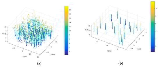
Figure 2.
Trunk points extraction. (a) Trunk points extraction result using transductive transfer learning; (b) trunk points optimization after removing misjudged points.
2.2.2. Canopy Points Projection Transformation Based on PCA Principle
The initial tree segmentation results were obtained using the extracted trunk centers. However, the initial segments are prone to under segmentation since the extracted trunk centers generally contain some omission errors. That is, some points belonging to two different trees may be clustered as one segment. Therefore, the initial tree segmentation results need further optimization for achieving better single tree extraction performance.
In this study, the canopy and trunk were extracted separately. To avoid the influence of trunks or low brushes, this study first removes the points below the highest trunk points within each initial segment for optimizing canopy points. This process can be written as Equation (3),
where represents the canopy points, is the point in the initial segment , is the number of points within , is the coordinate of and represents the maximum elevation of the trunk points.
As shown in Figure 3a, the canopy points of two adjacent trees are prone to be divided together. To achieve better individual tree extraction results, the undersegmented canopy points should be further separated. Generally speaking, the horizontal projection of canopy points of one single tree should be approximately circular. However, if more than one canopy is merged together, the corresponding canopy points’ horizontal projection tends to be elliptic as shown in Figure 3b.
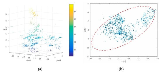
Figure 3.
Undersegmented canopy points. (a) Canopy points of two adjacent trees are divided together; (b) the horizontal projection of the under-segmented canopy points tend to be elliptic.
As can be seen from Figure 4a, compared with the points distribution in the x and y directions, the points are more distinct in the direction of the long axis of the ellipse (). Figure 4b is the projection of the points in the direction of the long axis of the ellipse. It is easy to find that the points after projection in direction are more distinct for separation.
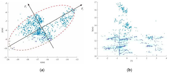
Figure 4.
Canopy points projection transformation based on PCA principle. (a) Canopy points distribution in x and y directions; (b) the projection of points in the direction of the long axis of the ellipse.
The direction of the long axis of an ellipse can usually be defined as the direction of the first principal component of the PCA method. Therefore, this paper first applied PCA principle to transform the canopy points. To avoid the interference of some isolated points on the calculation of principal component analysis, this paper calculates the number of neighboring points of each point. The points with a smaller number of neighboring points were determined as isolated points and removed. Then, the covariance tensor of each initial segment is calculated according to Equation (1). The eigenvalues and eigenvectors of the covariance tensor were also calculated. The direction of the eigenvector corresponding to the maximum eigenvalue is defined as the direction of the long axis of the ellipse, and the points are projected in this direction. The transformation process can be described by Equation (4),
where is the principal component after the transformation, is the matrix, and , , is the coordinates of in the (Equation (3)), is the total number of points that in the cluster. is the eigenvector matrix of the cluster’s covariance matrix.
2.2.3. The Number of Components Determination Based on Kernel Density Estimation
As mentioned above, the initial segmentation results based on the trunk centers are prone to be under segmentation. In other words, there may be more than one tree in one segment. As shown in Figure 4b, there are two mixed trees that need to be separated. It can also be found that to achieve optimal segmentation of canopies, it is necessary to first determine the number of mixed components within each initial cluster.
From Figure 4b, it can be found that the point density of the centers of each tree is usually large. Figure 5a,b are histograms of point density distribution of tree points in Figure 4b. The difference between Figure 5a,b is the different statistical interval of point density statistics in the direction, which is calculated based on PCA principle as described in Section 2.2.2. It is easy to find from these two figures that the point density from the centers to the two sides shows a downward trend. Therefore, the number of components can be determined by detecting the number of local maxima of point density. To accurately detect the local maximum of point density, the kernel density estimation method was used to calculate the probability density function distribution of each initial segment. The kernel density estimation is defined as Equation (5),
where is the number of points within each initial segmentation, is the bandwidth and is the kernel function. In this study, Gaussian kernel function was used for probability density estimation, which is defined in Equation (6) as:
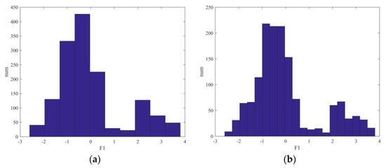
Figure 5.
Histograms of point density distribution with different statistical interval. (a) Statistical interval is 0.6; (b) Statistical interval is 0.3.
In Equation (5), bandwidth has a great influence on the result of Gaussian kernel density estimation.
Figure 6a,b shows the Gaussian kernel density estimation curves calculated by the points in Figure 4b with different bandwidth parameters. To achieve accurate Gaussian probability density estimation, this paper applies Silverman’s rule of thumb to perform adaptive bandwidth calculation, which has been defined in Equations (7) and (8),
where is the bandwidth of the i-th dimension, is the dimension, which is equal to 1 in this study and is the total number of points. is the estimated value of the standard deviation of the i-th dimension variable, and is the median of the absolute value of the residual difference between each variable and the mean value. The constant 0.6745 ensures that the estimation is unbiased under the normal distribution.
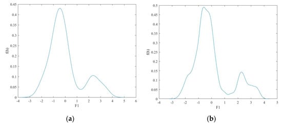
Figure 6.
Kernel density estimation curves of different bandwidths, the band width in (a) is 0.4, and the bandwidth in (b) is the value calculated according to Equation (10).
2.3. Canopy Points Extraction Through Gaussian Mixture Model Separation
From Figure 6 it can be found that the kernel density distribution curves of different trees that clustered together can be regarded as a mixture of different Gaussian distributions. Therefore, the optimal segmentation of different trees can be achieved by separating the mixed Gaussian models with different parameters. By detecting the number of local maxima of the kernel density distribution curve, it can be determined that Figure 4b has two components, as shown in Figure 7a. Then, the Gaussian mixture model separation method can be applied to divide the mixed canopy points into two clusters.
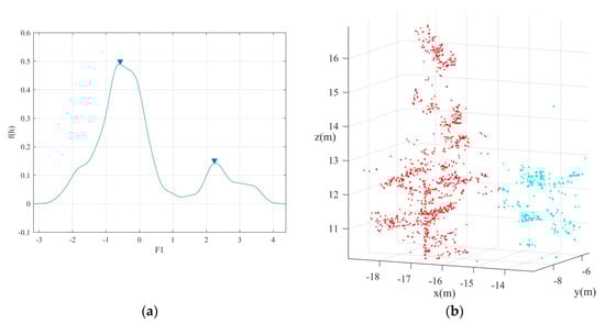
Figure 7.
Canopy points extraction through Gaussian mixture model separation. (a) The detection the number of local maxima of the kernel density distribution curve; (b) the separated results of the clustered canopy points, where points with red and green colors represent two separated trees.
In general, if the point clouds contain different clusters of points, the density function of the Gaussian mixture distribution can be written as Equation (9),
where represents vectors, which are the results of PCA transformation, that is . is the mixed components and is the coefficient of proportion, which represents the prior probability of each mixed components. are the parameters of the Gaussian distribution, and represent mean value, and variance, respectively. While, represents the Gaussian density function, which is defined in Equation (10) as:
The expected-maximum (EM) algorithm is used to estimate the parameters of the Gaussian mixture model, which mainly includes the ‘E’ step and ‘M’ step. The ‘E’ step tries to calculate the probability of each component, while the ‘M’ step updates the Gaussian mixture model parameters, including , and , where . is the number of mixed components.
The EM algorithm needs to be implemented repeatedly. The convergence condition of the iteration is that the variation of mixed distribution parameters calculated in the last iteration and calculated in the next iteration must be less than the threshold value, or the number of iterations reaches the maximum. When the EM algorithm stops iterating, the points are divided into categories according to the maximum probability that the points belongs to. The points in Figure 3a can be optimized as two separated tree canopies as shown in Figure 7b.
2.4. Over-Segmentation Canopies Optimization Based on Point Density Barycenter
The canopy points extracted by Gaussian mixture model separation may be over-segmentation. In other words, the canopy points of one tree may be segmented as two or more clusters. Moreover, in Section 2.1, the initial segmentation results were obtained based on the initial trunk centers. Since the initial trunk centers are not correct enough, one individual tree may also be divided into several trees mistakenly. This over-segmentation will not only make the extracted individual trees incomplete, but also lead to larger commission errors.
It is important to note that the horizontal positions of over-segmented trees are usually closer. Many researchers merge the over-segmented trees by calculating the horizontal distance of the highest points within each cluster, while some other researchers calculate the mean value of horizontal coordinates of each cluster to determine whether to combine the clusters. The above-mentioned two methods can obtain effective merging results under ideal conditions, such as the highest point of the tree is the vertex position of the tree, and the tree grows uniformly and symmetrically. However, in nature, due to the influence of light and water environments, the distribution of vegetation may be diverse. The highest point’s position or the mean coordinate of all points cannot represent the center of each cluster well. To make the forest optimization and combination method more robust, the barycenter of each cluster was proposed to combine the extracted trees close to each other.
As shown in Figure 8, the points’ distribution along the vertical direction of the center position of one individual tree is generally dense. Therefore, the planar position with the highest point density is more representative of the central location of the individual tree when comparing with the location of the vertex or mean coordinates of the tree points. In this study, this location is defined as the weighted average of point density distribution after horizontal projection of point clouds, which are represented in Equations (11)–(13),
where and are the number of grids after point clouds horizontal projection, as shown in Figure 8. is the horizontal coordinate of grid , is the coordinate of one point in grid . represents calculating the mean value. is the weight of grid . is the number of points with grid .
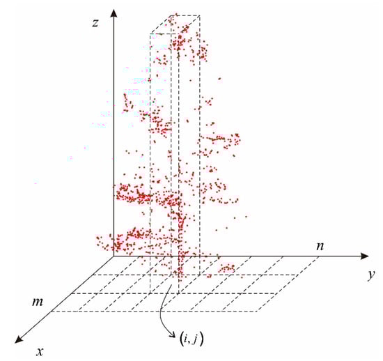
Figure 8.
The sketch map of the barycenter calculation.
2.5. Trunk Points Optimization in a Top-Down Manner
Although trunk points have been extracted by transductive transfer learning in Section 2.1, the number of extracted trunks is generally less than the reference number of trunks, which always lead to large omission error. To obtain better trunk extraction results, this paper tries to acquire trunk points based on the optimized canopy points for each individual tree that have been extracted in Section 2.4. Thus, the trunk points extraction method in this paper can also be called a top-down method.
According to the method mentioned in Section 2.3 and Section 2.4, the optimized canopy points can be extracted by separating Gaussian mixture model and merging strategy, as shown in Figure 9a. In this paper, the optimized trunk points are obtained in a top to down manner. Firstly, the horizontal projection range of the canopy points are obtained as and . Then, the points under the canopy can be acquired by subtracting the canopy points calculated in Equation (3), which is written as the point set . Finally, the points within the horizontal projection can be obtained according to Equation (14),
where represents the canopy points of -th individual tree as shown in Figure 9a. is the points under the canopy of each individual tree. Figure 9b is the combination of and . Obviously, the individual tree has been extracted successfully. However, there are still some low points in the extraction points, which are generally bushes. There points can be removed by voxelizing the point sets as shown in Figure 9c. The cubes with points falling in are labeled as 1. The number of cubes in each vertical direction is calculated. The points with poor continuity are filtered.
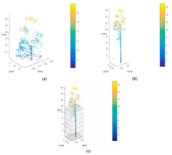
Figure 9.
Turnk points extraction based on the extracted canopy points. (a) The extracted canopy points; (b) the results of extracted individual tree; (c) low points removing by voxelizing.
3. Experimental Results and Analysis
3.1. Dataset
This paper adopts an international standard TLS dataset for evaluating the performance of the proposed method. The dataset is provided by the Finish Geospatial Research Institute (FGI), which can be used for non-profit research purpose [44]. The TLS point clouds were collected using Leica HDS1600 terrestrial laser scanner, which are located in southern boreal forests in Evo, Finland. The dataset contains many different vegetation types with different point densities. Thus, it will be representative for testing the effectiveness and robustness of the proposed method. The dataset contains six different plots, which has a fixed size ( square meter). In each plot, two scanning modes, namely single-scan and multi-scan are adopted to acquire the point clouds. According to the complexity of the forests in the plot, these six plots are classified as three categories, namely easy, medium and difficult types. The characteristics of these six plots are tabulated in Table 2. Figure 10 shows the six plots with the above-mentioned three types. In each plot, both single-scan and multi-scan acquired point clouds are contained.
Table 2.
Characteristics of the dataset [22,44].
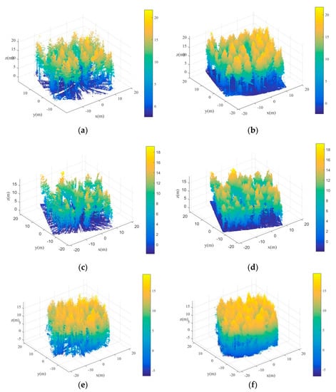
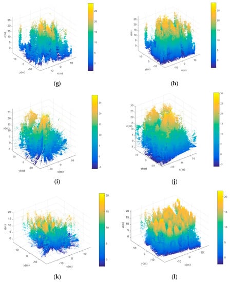
Figure 10.
Point clouds of six plots. (a,b) are point clouds of Plot 1; (c,d) are point clouds of Plot 2; (e,f) are point clouds of Plot 3; (g,h) are point clouds of Plot 4; (i,j) are point clouds of Plot 5; (k,l) are point clouds of Plot 6. The first column represents point clouds scanned in the single-scan mode, while the second column represents point clouds scanned in the multi-scan mode.
3.2. Accuracy Metrics Calculation
To evaluate the performance of the proposed method, this paper adopted the following steps to access the performance of the proposed method. The steps of the accuracy metrics calculation are shown in Table 3.
Table 3.
Accuracy metrics calculation steps.
Three indicators, including completeness (), correctness () and mean accuracy () are calculated for evaluating the performance of the proposed method according to Equations (15)–(17). The completeness reflects the detecting ability of the proposed method, while the correctness shows how many trees are correctly extracted. The average precision measures the joint probability that the randomly selected extraction tree is correct and that the randomly selected reference tree is detected by the method:
3.3. Experimental Results
In this paper, two individual tree point clouds with label information are used as the transfer learning source domain. The datasets are provided by Moorthy et al. [45], which are classified as wood and leaf points manually using an open source software named CloudCompare. The two individual tree point clouds were collected by Riegl VZ-400 and Riegl VZ-1000 terrestrial laser scanner, respectively. Figure 11a,b shows the two individual trees with label information. Although in transfer learning tree species in source and target domains may be different, wood points and leaf points have obviously different geometric features. In general, wood points present linear geometric features, while leaf points are usually scattered distribution. By calculating five geometric feature vectors of each point, the transfer learning model from source domain can be built. Then, the built model can be applied to the target domain of the above-mentioned six plots to classify the tree point clouds as wood and leaf points. After the trunk points optimization using the technique mentioned in Section 2.2.1, the trunk points of each plot with both single-scan and multi-scan modes can be extracted as shown in Figure 12. From Figure 12, it can be found that more trunk stems can be extracted from easy plots (Figure 12a–d) than the ones extracted from difficult plots (Figure 12i–l). It is because that the trees in the difficult plots are more dense and complicated as shown in Figure 10e,f. The linear geometric features of trunk points in the difficult plots are not significantly different from the ones of leaf points. Thus, many trunk stems cannot be detected effectively. Moreover, it can also be found that more tree stems can be extracted from the point clouds scanned in multi-scan mode than tree stems extracted from the point clouds scanned in single-scan mode. That makes sense because tree points acquired by multi-scan mode are more complete. Thus, linear geometric features of trunk stems are more obvious. However, it must be admitted that the tree stems extraction results are not very good, especially in difficult plots. The tree stems extraction results generally contain some omission errors. In this paper, the extracted tree stems only serves as the clustering centers for initial segmentation. Thus, the under-segmentation results can be optimized by the following Gaussian mixture model separation.
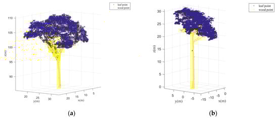
Figure 11.
Two individual trees point clouds with label information used for building transfer learning model. (a) An individual tree collected by Riegl VZ-400 terrestrial laser scanner; (b) An individual tree collected by Riegl VZ-1000 terrestrial laser scanner. Both of these two trees are classified as leaf and wood points manually. Blue points represent leaf points, while yellow points represent wood points.
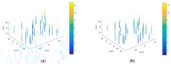
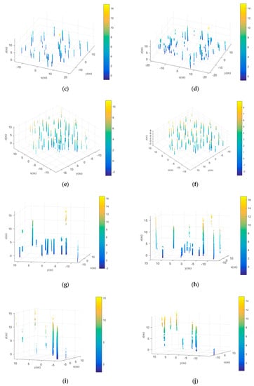
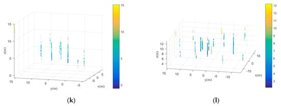
Figure 12.
Extracted trunk stems for the six plots scanned in both single-scan and multi-scan modes. (a,b) are the extracted stems for Plot 1; (c,d) are the extracted stems for Plot 2; (e,f) are the extracted stems for Plot 3; (g,h) are the extracted stems for Plot 4; (i,j) are the extracted stems for Plot 5; (k,l) are the extracted stems for Plot 6; the first column represents the single-scan mode, while the second column represents the multi-scan mode.
When the trunk stems are extracted, the initial clustering centers can be obtained by projecting the trunk points onto the horizontal plane. According to the clustering centers, the initial segmentation results can be obtained. As mentioned above, since the extracted trunk results generally contain omission errors, the initial tree segmentation results are always under-segmentation. After using the proposed techniques mentioned in Section 2.2.2, Section 2.2.3, Section 2.3 and Section 2.4, the under-segmentation canopies can be separated correctly. Then, the trunks points corresponding to each individual canopy can be extracted in a top-down manner based on the vertical continuity principle. Figure 13 shows some instances of the extracted individual trees by the proposed method.
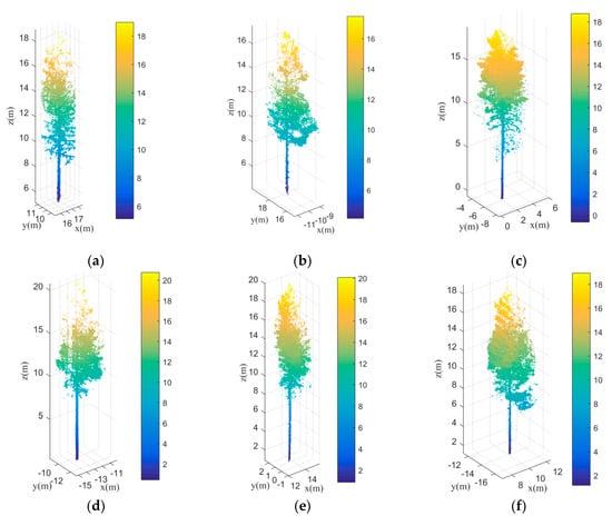
Figure 13.
Nine instances of extracted individual tree. (a–i) are the extracted individual trees.
From Figure 13, it can be found that the individual trees can be extracted correctly. In this paper, canopy extraction for each individual tree can be seen as a bottom-up process. It is because the trunk points are first classified from point clouds by transfer learning. Then Canopy points for each individual tree are extracted based on the initial segmentation using the extracted trunk centers. When the canopies are separated correctly, the trunk stem corresponding to each canopy is extracted in a top-down manner. Therefore, the proposed method in this paper can be seen as a combination of bottom-up and top-down approaches. As shown in Figure 13, both canopies and trunk stems for each individual tree can be extracted correctly.
Liang et al. [44] also provided the reference tree locations for the six plots. Thus, it is will be easy to access the performance of the proposed method towards different forest environments and scanning modes. Figure 14 shows the locations of the extracted trees and reference trees. From these figures, it can be found that although some reference trees cannot be detected, most of the extracted trees are correct. Only a few extracted trees are wrongly detected. Moreover, more trees can be extracted correctly in the point clouds scanned in multi-scan mode than in the point clouds scanned in single-scan mode. That makes sense because multi-scan mode can provide more complete tree points. Another point to be noted is that as the forest scenes become more complex, fewer trees can be extracted effectively. As shown in Figure 14, more trees can be extracted in easy plots (Figure 14a–d) than in medium and difficult plots (Figure 14e–l). It is because the forest density of medium and difficult plot is much larger than that of easy plot as tabulated in Table 2. Obviously, dense trees are not easy to be extracted. Besides, trees in the easy plots are intuitively easier to be separate as shown in Figure 10.
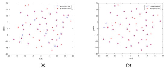
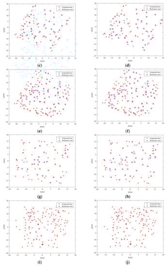
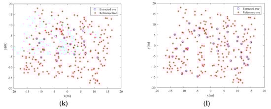
Figure 14.
Horizontal locations of the extracted and reference trees for the six plots scanned in both single-scan and multi-scan modes. (a,b) are the locations of the extracted stems for Plot 1; (c,d) are the locations of the extracted stems for Plot 2; (e,f) are the locations of the extracted stems for Plot 3; (g,h) are the locations of the extracted stems for Plot 4; (i,j) are the locations of the extracted stems for Plot 5; (k,l) are the locations of the extracted stems for Plot 6; the first column represents the single-scan mode, while the second column represents the multi-scan mode.
3.4. Comparison and Analysis
To quantitatively evaluate the performance of the proposed method, this paper calculated the three indicators, namely completeness, correctness and mean accuracy for the six plots according to the Equations (15)–(17). Meanwhile, two other individual tree extraction methods are also tested to compare the accuracy metrics with the ones of the proposed method. The first method is the marker-controlled watershed segmentation, which was implemented in a Digital Forestry Toolbox. The Digital Forestry Toolbox is realized using the Matlab programming language, which is developed for analyzing LiDAR data related to forests. In this method, the treetops are detected using variable window sizes, which can be estimated based on the regression curve between crown size and tree height. The treetops are then selected as the markers for watershed segmentation to prevent over segmentation. The second classical individual tree extraction method was implemented in a LiDAR processing software named LiDAR360. In this method, individual trees are separated based on the horizontal spacing between trees. Generally speaking, the horizontal spacing between trees at the top is larger than the horizontal spacing at the bottom. Therefore, the individual tree points can be grown from the tree tops based on the relative spacing between trees. In other words, the points of a same tree can be added gradually since its relative spacing is smaller, while the points of other trees will be excluded since its relative spacing is larger.
Table 4 shows the accuracy metrics calculation results of the proposed method towards the six plots. In each plot, both single-scan (SS) and multi-scan (MS) modes are included. From Table 4, it can be found that the proposed method can achieve high correctness of the extracted trees. Almost the correctness of all the plots is higher than 80%. As a result, the average of the correctness of the six plots containing both single-scan and multi-scan modes is 87.68%. Another finding is the same as the conclusion drawn by Liang et al. (2018) that the higher correctness is generally at the cost of lower completeness. The average of completeness of the proposed method is 37.33%. Compared with correctness and completeness, mean accuracy is a relatively balanced precision index. In terms of mean accuracy, the proposed method can achieve 69.85% average of mean accuracy for easy plots, 57.36% average of mean accuracy for medium plots and 18.57% average of mean accuracy for difficult plots. Therefore, a same conclusion here can be drawn as from Figure 14 that the performance of the proposed method will turn down as the forest environments changed to be complicated.
Table 4.
Three accuracy indicators calculation results of the proposed method towards the six plots. In each plot, both single-scan (SS) and multi-scan (MS) modes are included.
Figure 15, Figure 16 and Figure 17 show the comparison of completeness, correctness and mean accuracy of the proposed method and the other two methods developed in the Digital Forestry Toolbox and LiDAR360. In terms of completeness (Figure 15), the proposed method outperforms the other two methods in all the plots except plot_5_SS and plot_6_SS. As a result, the average completeness of the proposed method is much higher than that of the other two methods. In terms of correctness (Figure 16), the proposed method performs much better than the other two methods. Almost all the correctness of the plots in this paper is higher than 80%, while the maximum correctness of the other two methods is less than 40%. Combining completeness and correctness as shown in Figure 15 and Figure 16, it can be concluded that the proposed method can extract more trees while ensuring a high accuracy of tree extraction. In terms of mean accuracy (Figure 17), the proposed method performs much better than the other two methods. Moreover, all the three methods achieve worse mean accuracy as the forest environments change from easy to difficult. Thus, it can be concluded that dense and complex forest environments still pose great challenges to the individual tree extraction methods.
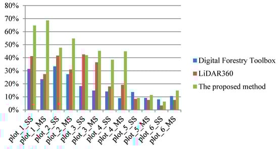
Figure 15.
Comparison of completeness of the three methods towards the six plots.
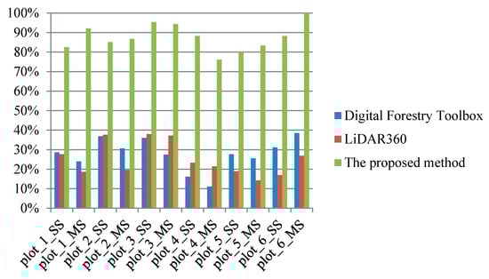
Figure 16.
Comparison of correctness of the three methods towards the six plots.
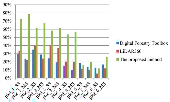
Figure 17.
Comparison of mean accuracy of the three methods towards the six plots.
Another dataset used in practice was also adopted for testing the performance of the proposed method. The dataset was acquired using the Riegl VZ-400 scanner, which can obtain dense point clouds accurately. After the scanned point clouds are preprocessed by Riscan pro software and filtered, the normalized point clouds for the tree plot are shown in Figure 18a. From Figure 18a, it can be found that the trees in this plot are dense. Many adjacent trees are very close. Moreover, there are some small trees that are under the canopy of some tall trees. Therefore, this plot will be representative to show the effectiveness of the proposed method. All the trees in Figure 18a are separated manually using the CloudCompare software. The separation results by the proposed method are shown in Figure 18b. From Figure 18b, it can be observed that most trees are separated correctly. Among the 25 reference trees, 23 trees are extracted correctly by the proposed method. The completeness is 92%. Although most trees are detected successfully, there are still some trees that are over-segmented. 28 trees are extracted by the proposed method. Obviously, there are some trees are wrongly detected. The over-segmented trees are mainly caused by the trees with irregular canopies. In terms of this plot, the correctness is 82.14%. As a result, the mean accuracy of the proposed method is 86.79%.
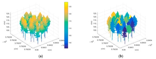
Figure 18.
Tree point cloud and its segmentation results. (a) Tree point clouds scanned by the Riegl VZ-400 terrestrial laser scanner; (b) segmented individual trees by the proposed method. Each segmented tree is random colored.
4. Discussion
In this paper, trunk stems are first detected by the transductive transfer learning, which are the key to the initial segmentation. It is because the initial segmentation is obtained by nearest neighbor clustering based on the acquired trunk stem centers. Table 5 shows the trunk stems detection rate by the transductive transfer learning for different plots. It is easy to find that the trunk stem detection rate turns worse as the forest environments become complicated, which is similar to the regularity of individual tree extraction results. Thus, it can be concluded that the trunk stems detection results have an influence of the final individual tree extraction results. Although the initial segmentation results can be optimized by the following Gaussian mixture model separation, the individual tree extraction results cannot be good if the initial segmentation results are too poor. Figure 19a shows an initial segmentation for an easy plot (Plot 1). It is easy to find that although some adjacent trees are clustered together in the initial segmentation, the segmentation results still show clear difference among separated trees. The under-segmentation for some adjacent trees can be easy to be further separated by the following steps in this paper. As a contrast, Figure 19a shows an initial segmentation for a difficult plot (Plot 6). From this figure, it is difficult to find separated trees. Although both Figure 19a,b are under-segmentation, Figure 19b cannot be further revised well since its initial segmentation is too poor.
Table 5.
Trunk stems detection rate by the transductive transfer learning for different plots.
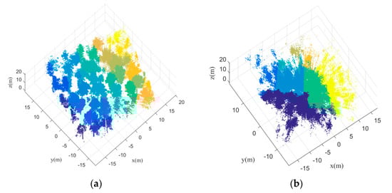
Figure 19.
Initial segmentation results for easy and difficult plots. (a) Plot 1 scanned in single mode; (b) plot 6 scanned in single mode.
As mentioned above, some adjacent trees may be clustered together in the initial segmentation results. These under-segmented trees need to be further separated. Thus, the Gaussian mixture model separation plays an important role in the separation to under-segmented canopies. In the Gaussian mixture model separation, the separation number has a direct influence on the separation results. Figure 20 shows the different separation results towards different separation number by applying the Gaussian mixture model separation. Clearly, if the separation number is larger than the number of reference trees, the separation results are over-segmentation. If the separation number is smaller than the number of reference trees, the separation results are under-segmentation. Therefore, the accurate separation number should be determined. In this paper, the separation number can be calculated based on kernel density estimation. By detecting the number of local maxima of the kernel density distribution curve, the number of mixed components can be acquired automatically.
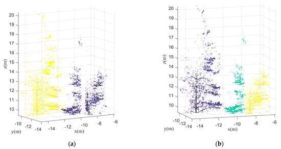
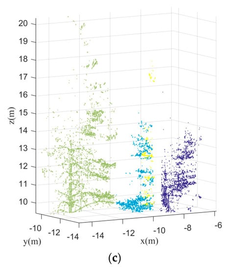
Figure 20.
Separation results towards different separation number by applying the Gaussian mixture model separation. (a) The separation number is 2; (b) the separation number is 3; (c) the separation number is 4.
Although the under-segmented trees can be revised by the Gaussian mixture model separation, the trees that grow under another tree’s canopy are still difficult to be separated by the EM algorithm. Figure 21a,b are two instances of the individual tree extraction results. Clearly, the extraction results contain omission errors. The smaller trees were not detected effectively. The reasons for this are twofold. On the one hand, the separation number cannot be calculated accurately based on kernel density estimation since the local maxima of the kernel density distribution curve formed by the smaller trees cannot be detected effectively. On the other hand, the Gaussian mixture model separation method is easy to misclassify trees that grow too much closer to be one tree. How to detect the trees that grow under canopies need to be focused in our future research. In terms of the trees with complex canopy architectures, such as the broadleaf forests, the proposed method will encounter difficulties. It is because the trees separation in this research mainly depends on the kernel density distribution of the canopy points. If the canopy architectures are complicated, the number of the local maxima of the kernel density distribution will not correspond to the number of trees that need to be segmented. Thus, the following individual trees segmentation using the EM algorithm will not be correct.
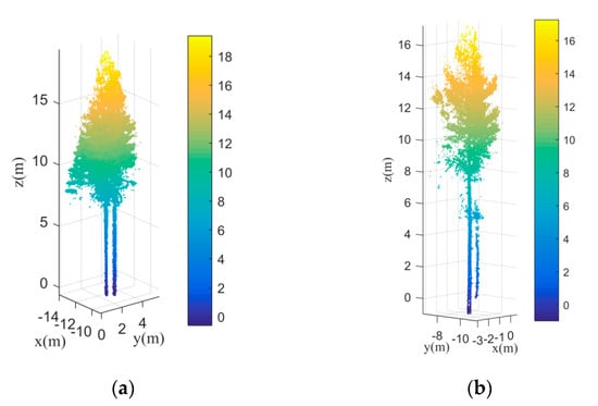
Figure 21.
The wrongly separated individual trees and (a,b) are two examples of the smaller trees that cannot be detected accurately.
5. Conclusions
To improve the accuracy of individual tree extraction, this paper proposed a novel method based on transfer learning and Gaussian mixture model separation. As a whole, the proposed method can be seen as a process of the combination of bottom-up and top-down manners. In the bottom-up manner, the trunk points are first classified from point clouds using the transfer learning. The extracted trunk points can then be served as clustering centers for initial segmentation. Based on PCA transformation, kernel density estimation and Gaussian mixture model separation, the canopy for each individual tree can be extracted correctly. In the top-down manner, the extracted canopies are served as guidance for trunk stems extraction. The trunk stems are extracted according to the vertical continuity. Six plots with different forest environments are used for testing the performance of the proposed method. The experimental results show that the transfer learning can be used for trunk points classification. Although the classification results may contain omission errors, the trunk points can still be used for initial tree segmentation. The under segmentation canopies in the initial tree segmentation can be optimized successfully using Gaussian mixture model separation. As a result, the proposed method can achieve 87.68% average correctness towards the six plots with single-scan and multi-scan modes, which is much higher than that of the other two classical methods. In terms of completeness and mean accuracy, the proposed method also outperforms the other two methods. Therefore, the proposed method can extract more trees while ensuring a high accuracy of tree extraction.
Author Contributions
Z.H. conceived the original idea of the study and drafted the manuscript. S.J. and Y.Y.Z. contributed to the revision of the manuscript. D.L. and B.L. performed the experiments and made the experimental analysis. All authors have read and agreed to the published version of the manuscript.
Funding
This work was supported by the China Post-Doctoral Science Foundation (2019M661858), the National Natural Science Foundation of China (NSF) (41801325), the Natural Science Foundation of Jiangxi Province (20192BAB217010), Education Department of Jiangxi Province (GJJ170449), Key Laboratory for Digital Land and Resources of Jiangxi Province, East China University of Technology (DLLJ201806), East China University of Technology Ph. D. Project (DHBK2017155) for their financial support.
Data Availability Statement
The publicly datasets tested in this paper can be found from the following links: http://laserscanning.fi/tls-benchmarking-results/.
Acknowledgments
Authors would like to thank the Finish Geospatial Research Institute for providing abundant datasets located in different forest environments.
Conflicts of Interest
The authors declare no conflict of interest.
Appendix A
Detailed steps for misjudged leaf points removal:
Firstly, the points were voxelized. Figure A1a,b are the voxelized results for trunk points and misjudged points, respectively. It is easy to find that the trunk points have a strong continuity in the vertical direction. Thus, there are fewer empty cubes in the vertical direction as shown in Figure A1a. For the misjudged points, there are more empty cubes in the vertical direction (Figure A1b). On the basis of this, most misjudged points with poor vertical continuity can be eliminated. In addition, according to the characteristic feature that the misjudged points are usually scattered, the misjudged points can be further eliminated by clustering with neighboring points. The points with small number of neighboring points were removed as misjudged points.

Figure A1.
Comparison of continuity in the vertical direction between the trunk points and the misjudged points. (a) Trunk points; (b) Misjudged points.
Figure A1.
Comparison of continuity in the vertical direction between the trunk points and the misjudged points. (a) Trunk points; (b) Misjudged points.

Appendix B
Detailed steps for Trunk centers optimization:
In this paper, the points of each trunk were first projected horizontally with the projected points divided into grids afterwards (Figure A2a). As can be seen in Figure A2a, after the horizontal projection the distribution of trunk points was relatively concentrated, while the distribution of burr points was relatively sparse. Therefore, the burr points mixed with the trunk points were eliminated based on the point density constraint. In this paper, the threshold of point density constraint was set as the average number of points in each grid, which can be calculated as Equation (A1):
where is the point density constraint threshold, is the two-dimensional grid, which is formed by the horizontal projection of the trunk points, is the number of points that in each two-dimensional grid. and are the maximum values in the horizontal and vertical direction of the two-dimensional grid, and represents mean value. and are the and coordinates of each trunk point , and are the grid coordinates of point in the two-dimensional grid. represents downward rounding. The trunk points after removing burr points can be represented as Equation (A2).
The points of each trunk after removing burr points are shown in Figure 4b. It can be found that the burr points on the trunks were effectively removed.

Figure A2.
Burr points removal using horizontal projection under point density constrain. (a) Horizontal projection of trunk points; (b) Burr points removal results after point density constrain.
Figure A2.
Burr points removal using horizontal projection under point density constrain. (a) Horizontal projection of trunk points; (b) Burr points removal results after point density constrain.

After removing the burr points, the trunk center horizontal position was calculated as Equation (A3).
where is the horizontal position of the i-th trunk center, are the and coordinates of the i-th trunk after removing burr points and are the number of points of the i-th trunk.
References
- Shan, J.; Toth, C.K. Topographic Laser Ranging and Scanning: Principles and Processing; CRC Press: Boca Raton, FL, USA, 2008. [Google Scholar]
- Vosselman, G.; Maas, H.G. Airborne and Terrestrial Laser Scanning; DBLP: Scotland, UK, 2010. [Google Scholar]
- Dong, P.; Chen, Q. LiDAR Remote Sensing and Applications; CRC Press: Boca Raton, FL, USA, 2018. [Google Scholar]
- Hui, Z.; Lia, D.; Jin, S.; Ziggah, Y.Y.; Wang, L.; Hud, Y. Automatic DTM extraction from airborne LiDAR based on expectationmaximization. Opt. Laser Technol. 2019, 112, 43–55. [Google Scholar] [CrossRef]
- Zhao, K.; Suarez, J.C.; Garcia, M.; Hu, T.; Wang, C.; Londo, A. Utility of multitemporal lidar for forest and carbon monitoring: Tree growth, biomass dynamics, and carbon flux. Remote Sens. Environ. 2018, 204, 883–897. [Google Scholar] [CrossRef]
- Chen, C.; Wang, M.; Chang, B.; Li, Y. Multi-Level Interpolation-Based Filter for Airborne LiDAR Point Clouds in Forested Areas. IEEE Access 2020, 8, 41000–41012. [Google Scholar] [CrossRef]
- Hyyppa, J.; Hyyppa, H.; Leckie, D.; Gougeon, F.; Yu, X.; Maltamo, M. Review of methods of small-footprint airborne laser scanning for extracting forest inventory data in boreal forests. Int. J. Remote Sens. 2008, 29, 1339–1366. [Google Scholar] [CrossRef]
- Xiao, W.; Xu, S.; Elberink, S.O.; Vosselman, G. Individual Tree Crown Modeling and Change Detection from Airborne Lidar Data. IEEE J. Sel. Top. Appl. Earth Obs. Remote Sens. 2016, 9, 3467–3477. [Google Scholar] [CrossRef]
- Bigdeli, B.; Amirkolaee, H.A.; Pahlavani, P. DTM extraction under forest canopy using LiDAR data and a modified invasive weed optimization algorithm. Remote Sens. Environ. 2018, 216, 289–300. [Google Scholar] [CrossRef]
- Yu, X.; Liang, X.; Hyyppa, J.; Kankare, V.; Vastaranta, M.; Holopainen, M. Stem biomass estimation based on stem reconstruction from terrestrial laser scanning point clouds. Remote Sens. Lett. 2013, 4, 344–353. [Google Scholar] [CrossRef]
- Kankare, V.; Holopainen, M.; Vastaranta, M.; Puttonen, E.; Yu, X.; Hyyppa, J.; Vaaja, M.; Hyyppa, H.; Alho, P. Individual tree biomass estimation using terrestrial laser scanning. ISPRS J. Photogramm. 2013, 75, 64–75. [Google Scholar] [CrossRef]
- Astrup, R.; Ducey, M.J.; Granhus, A.; Ritter, T.; von Lupke, N. Approaches for estimating stand-level volume using terrestrial laser scanning in a single-scan mode. Can. J. For. Res. 2014, 44, 666–676. [Google Scholar] [CrossRef]
- Liang, X.; Kankare, V.; Yu, X.; Hyyppa, J.; Holopainen, M. Automated Stem Curve Measurement Using Terrestrial Laser Scanning. IEEE Trans. Geosci. Remote 2014, 52, 1739–1748. [Google Scholar] [CrossRef]
- Xu, S.; Ye, N.; Xu, S.; Zhu, F. A supervoxel approach to the segmentation of individual trees from LiDAR point clouds. Remote Sens. Lett. 2018, 9, 515–523. [Google Scholar] [CrossRef]
- Jaafar, W.S.W.M.; Woodhouse, I.H.; Silva, C.A.; Omar, H.; Maulud, K.N.A.; Hudak, A.T.; Klauberg, C.; Cardil, A.; Mohan, M. Improving Individual Tree Crown Delineation and Attributes Estimation of Tropical Forests Using Airborne LiDAR Data. Forests 2018, 9, 759. [Google Scholar] [CrossRef]
- Wang, Y.; Pyorala, J.; Liang, X.; Lehtomaki, M.; Kukko, A.; Yu, X.; Kaartinen, H.; Hyyppa, J. In Situ Biomass Estimation at Tree and Plot Levels: What Did Data Record and What Did Algorithms Derive from Terrestrial and Aerial Point Clouds in Boreal Forest. Remote Sens. Environ. 2019, 232, 11309. [Google Scholar] [CrossRef]
- Lin, Y.; Hyyppa, J.; Jaakkola, A.; Yu, X. Three-level frame and RD-schematic algorithm for automatic detection of individual trees from MLS point clouds. Int. J. Remote Sens. 2012, 33, 1701–1716. [Google Scholar] [CrossRef]
- Srinivasan, S.; Popescu, S.C.; Eriksson, M.; Sheridan, R.D.; Ku, N. Terrestrial Laser Scanning as an Effective Tool to Retrieve Tree Level Height, Crown Width, and Stem Diameter. Remote Sens. 2015, 7, 1877–1896. [Google Scholar] [CrossRef]
- Henning, J.G.; Radtke, P.J. Detailed stem measurements of standing trees from ground-based scanning lidar. For. Sci. 2006, 52, 67–80. [Google Scholar]
- Strimbu, V.F.; Strimbu, B.M. A graph-based segmentation algorithm for tree crown extraction using airborne LiDAR data. ISPRS J. Photogramm. 2015, 104, 30–43. [Google Scholar] [CrossRef]
- Lee, H.; Slatton, K.C.; Roth, B.E., Jr.; Cropper, W.P. Adaptive clustering of airborne LiDAR data to segment individual tree crowns in managed pine forests. Int. J. Remote Sens. 2010, 31, 117–139. [Google Scholar] [CrossRef]
- Zhang, W.; Wan, P.; Wang, T.; Cai, S.; Chen, Y.; Jin, X.; Yan, G. A Novel Approach for the Detection of Standing Tree Stems from Plot-Level Terrestrial Laser Scanning Data. Remote Sens. 2019, 11, 211. [Google Scholar] [CrossRef]
- Liang, X.; Litkey, P.; Hyyppa, J.; Kaartinen, H.; Vastaranta, M.; Holopainen, M. Automatic Stem Mapping Using Single-Scan Terrestrial Laser Scanning. IEEE Trans. Geosci. Remote 2012, 50, 661–670. [Google Scholar] [CrossRef]
- Liang, X.; Kukko, A.; Hyyppa, J.; Lehtomaki, M.; Pyorala, J.; Yu, X.; Kaartinen, H.; Jaakkola, A.; Wang, Y. In-situ measurements from mobile platforms: An emerging approach to address the old challenges associated with forest inventories. ISPRS J. Photogramm. 2018, 143, 97–107. [Google Scholar] [CrossRef]
- Olofsson, K.; Holmgren, J.; Olsson, H. Tree Stem and Height Measurements using Terrestrial Laser Scanning and the RANSAC Algorithm. Remote Sens. 2014, 6, 4323–4344. [Google Scholar] [CrossRef]
- Jakubowski, M.K.; Li, W.; Guo, Q.; Kelly, M. Delineating Individual Trees from Lidar Data: A Comparison of Vector- and Raster-based Segmentation Approaches. Remote Sens. 2013, 5, 4163–4186. [Google Scholar] [CrossRef]
- Eysn, L.; Hollaus, M.; Lindberg, E.; Berger, F.; Monnet, J.; Dalponte, M.; Kobal, M.; Pellegrini, M.; Lingua, E.; Mongus, D.; et al. A Benchmark of Lidar-Based Single Tree Detection Methods Using Heterogeneous Forest Data from the Alpine Space. Forests 2015, 6, 1721–1747. [Google Scholar] [CrossRef]
- Hui, Z.; Jin, S.; Cheng, P.; Ziggah, Y.Y.; Wang, L.; Wang, Y.; Hu, H.; Hu, Y. An Active Learning Method for DEM Extraction from Airborne LiDAR Point Clouds. IEEE Access 2019, 7, 89366–89378. [Google Scholar] [CrossRef]
- Xiao, W.; Zaforemska, A.; Smigaj, M.; Wang, Y.; Gaulton, R. Mean Shift Segmentation Assessment for Individual Forest Tree Delineation from Airborne Lidar Data. Remote Sens. 2019, 11, 1263. [Google Scholar] [CrossRef]
- Zhen, Z.; Quackenbush, L.J.; Zhang, L. Impact of Tree-Oriented Growth Order in Marker-Controlled Region Growing for Individual Tree Crown Delineation Using Airborne Laser Scanner (ALS) Data. Remote Sens. 2014, 6, 555–579. [Google Scholar] [CrossRef]
- Hyyppa, J.; Kelle, O.; Lehikoinen, M.; Inkinen, M. A segmentation-based method to retrieve stem volume estimates from 3-D tree height models produced by laser scanners. IEEE Trans. Geosci. Remote 2001, 39, 969–975. [Google Scholar] [CrossRef]
- Chen, Q.; Baldocchi, D.; Peng, G.; Kelly, M. Isolating Individual Trees in a Savanna Woodland using Small Footprint LIDAR data. Photogramm. Eng. Remote Sens. 2006, 72, 923–932. [Google Scholar] [CrossRef]
- Mongus, D.; Zalik, B. An efficient approach to 3D single tree-crown delineation in LiDAR data. ISPRS J. Photogramm. 2015, 108, 219–233. [Google Scholar] [CrossRef]
- Yang, J.; Kang, Z.; Cheng, S.; Yang, Z.; Akwensi, P.H. An Individual Tree Segmentation Method Based on Watershed Algorithm and Three-Dimensional Spatial Distribution Analysis from Airborne LiDAR Point Clouds. IEEE J. Sel. Top. Appl. Earth Obs. Remote Sens. 2020, 13, 1055–1067. [Google Scholar] [CrossRef]
- Hu, X.; Wei, C.; Xu, W. Adaptive Mean Shift-Based Identification of Individual Trees Using Airborne LiDAR Data. Remote Sens. 2017, 9, 148. [Google Scholar] [CrossRef]
- Dai, W.; Yang, B.; Dong, Z.; Shaker, A. A new method for 3D individual tree extraction using multispectral airborne LiDAR point clouds. ISPRS J. Photogramm. 2018, 144, 400–411. [Google Scholar] [CrossRef]
- Cheng, Y.Z. Mean shift, mode seeking, and clustering. IEEE Trans. Pattern Anal. 1995, 17, 790–799. [Google Scholar] [CrossRef]
- Ferraz, A.; Bretar, F.; Jacquemoud, S.; Gonçalves, G.; Pereira, L.; Margarida Tomé G, P.S. 3-D mapping of a multi-layered Mediterranean forest using ALS data. Remote Sens. Environ. 2012, 121, 210–223. [Google Scholar] [CrossRef]
- Ferraz, A.; Saatchi, S.; Mallet, C.; Meyer, V. Lidar detection of individual tree size in tropical forests. Remote Sens. Environ. 2016, 183, 318–333. [Google Scholar] [CrossRef]
- Wei, C.; Hu, X.; Wen, C.; Hong, Y.; Yang, M. Airborne LiDAR Remote Sensing for Individual Tree Forest Inventory Using Trunk Detection-Aided Mean Shift Clustering Techniques. Remote Sens. 2018, 10, 1078. [Google Scholar]
- Li, W.; Guo, Q.; Jakubowski, M.K.; Kelly, M. A New Method for Segmenting Individual Trees from the Lidar Point Cloud. Photogramm. Eng. Remote Sens. 2012, 78, 75–84. [Google Scholar] [CrossRef]
- Zhong, L.; Cheng, L.; Xu, H.; Wu, Y.; Chen, Y.; Li, M. Segmentation of Individual Trees from TLS and MLS Data. IEEE J. Sel. Top. Appl. Earth Obs. Remote Sens. 2017, 10, 774–787. [Google Scholar] [CrossRef]
- Hui, Z.; Hu, Y.; Yevenyo, Y.Z.; Yu, X. An Improved Morphological Algorithm for Filtering Airborne LiDAR Point Cloud Based on Multi-Level Kriging Interpolation. Remote Sens. 2016, 8, 35. [Google Scholar] [CrossRef]
- Liang, X.; Hyyppa, J.; Kaartinen, H.; Lehtomaki, M.; Pyorala, J.; Pfeifer, N.; Holopainen, M.; Brolly, G.; Pirotti, F.; Hackenberg, J.; et al. International benchmarking of terrestrial laser scanning approaches for forest inventories. ISPRS J. Photogramm. 2018, 144, 137–179. [Google Scholar] [CrossRef]
- Moorthy, S.M.K.; Calders, K.; Vicari, M.B.; Verbeeck, H. Improved Supervised Learning-Based Approach for Leaf and Wood Classification from LiDAR Point Clouds of Forests. IEEE Trans. Geosci. Remote 2020, 58, 3057–3070. [Google Scholar] [CrossRef]


Publisher’s Note: MDPI stays neutral with regard to jurisdictional claims in published maps and institutional affiliations. |
© 2021 by the authors. Licensee MDPI, Basel, Switzerland. This article is an open access article distributed under the terms and conditions of the Creative Commons Attribution (CC BY) license (http://creativecommons.org/licenses/by/4.0/).