Estimation of Urban Ecosystem Services Value: A Case Study of Chengdu, Southwestern China

Abstract

Research on the service values of urban ecosystems is a hot topic of ecological studies in the current era of rapid urbanization. To quantitatively estimate the ecosystem service value in Chengdu, China from the perspectives of natural ecology and social ecology, the technologies of remote sensing (RS) and geographic information system (GIS) are utilized in this study to extract the land use type information from RS images of Chengdu in 2003, 2007, 2013 and 2018. Subsequently, a driver analysis of the ecosystem services of Chengdu was performed based on socioeconomic data from the last 16 years. The results indicated that: (1) from 2003 to 2018, the land utilization in Chengdu changed significantly, with the area of cultivated lands, forest lands and water decreasing remarkably, while the area of construction lands dramatically increased. (2) The ecosystem services value (ESV) of Chengdu decreased by 30.92% in the last 16 years, from CNY 2.4078 × 10¹⁰ in 2003 to CNY 1.6632 × 10¹⁰ in 2018. Based on a future simulation, the ESV is further predicted to be reduced to CNY 1.4261 × 10¹⁰ by 2033. (3) The ESV of Chengdu showed a negative correlation with the total population, the urbanization rate and the per capita GDP of the region, indicating that the ESV of the studied region was inter-coupled with the socioeconomic development and can be maintained at a high level through rationally regulating the socioeconomic structure.

1. Introduction

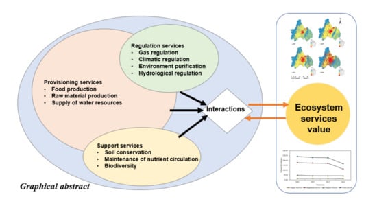
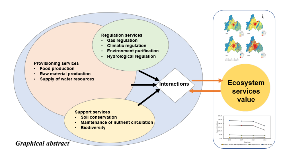
Ecosystem services refer to the natural environmental conditions and effects that humans rely on for survival, which are formed and maintained by ecosystems and their ecological processes [1]. It is often difficult to obtain a clear understanding of the importance and abundance/scarcity of ecosystem service functions only from the perspective of amount of substance [2]. Ecosystem service values refer to the values of life support products and services, provided directly or indirectly through the structure, process and functions of the ecosystem. The calculation of ecological service value provides a scientific basis for evaluating the quality of human life and production, the level of social sustainable development and green Gross Domestic Product (GDP), with important practical significance and scientific value. The quantitative evaluation of ecosystem service values for improving the public’s awareness of ecological and environmental protection is gradually becoming a major research topic [3].

Since the 20th century, one of the biggest changes in human society is urbanization. On the one hand, maintaining a city requires the consumption of a large amount of natural resources. On the other hand, due to the increasing urban population, there is an increase in land degradation, pervasive ground water contamination and intensive greenhouse gas (GHG) emissions [4], and a large volume of waste is discharged from the city into the surrounding environment [5].

Until now, studies conducted on the relationship between urbanization and ecosystem services have mainly focused on the impacts of urbanization on ecosystem services and the correlation between the two [6], e.g., how urbanization affects ecosystem services provided by water ecosystems, soil ecosystems [7], agroforest ecosystems [8], cultural ecosystems [9], and urban ecosystems [10]. The balance and collaboration between ecosystem services and social interaction and well-being have also attracted significant attention [11]. For example, Aguilera et al. [12] found that ecosystem services are compromised by progressive loss of natural connectivity and poor governance structure, which confer high vulnerability to urbanized bays with future urban expansion. Natasha et al. [13] analyzed the cities in Vhembe of South Africa and discussed the relationship between urbanization and forest restoration and its impact on the diversity of ecosystem services and the value of ecological restoration. Four key ecosystem service functions were quantified and analyzed to evaluate the impact of Beijing-Tianjin-Hebei urbanization on ecosystem services from 2000 to 2010 [14]. As for the temporal and spatial dynamics of urban ecosystem services, [15] assessed the impact of the urbanization of Bornova on the potential ecosystem services of urban and rural areas based on the existing spatial mapping method of potential ecosystems. However, in the studies on the correlation between urbanization and ecosystem services, the focus is mainly laid on the regulation of ecosystem services by urban planning, as well as the bidirectional interactions between urbanization and ecosystem services.

In the aspect of studies on ecosystem services for natural elements, Costanza et al. evaluated the ecosystem service value on a global scale in 1997 and gave specific functional classifications of ecosystem services [16]. Andersson-Sköld et al. raised six key questions in the review of urban ecosystem services and conducted related studies [17]; Ranta et al. analyzed the ecological impact of palm land on urban green space and greening so as to study the impact of palm land on urban ecosystem services [18]. Yongxiu et al. proposed this study of the four-quadrant model of human activities on the ecosystem service functions of the Qinghai-Tibet Park in 2020, which is helpful to explore the impact of human activities on ecosystem services [19]. Rawat et al. proposed the impact of vegetation and soil characteristics on ecosystem services [20], and Schirpke et al. proposed the relevance of land use changes on ecosystem services from the past to the future [21]. Lin et al. modified the method according to the actual conditions in China, and established a table of service equivalent factors per unit area of China’s terrestrial ecosystem [22]. Via comprehensively utilizing technologies including geographic information system (GIS) and remote sensing (RS), Affek et al., based on the characteristics of land use changes in Longquanyi District from 2003 to 2014, used Costanza’s method for estimating the ecosystem service value to estimate the changes in the ecosystem service value in Longquanyi District [23]. Using Landsat TM RS images and including forests and grasslands and their impacts on the ecosystem service value [24], Vaz et al. used the entropy method to evaluate the urbanization level of oasis-type cities, and obtained the correlation between the urbanization level and the ecosystem service value [25]. Song et al. used GF-2 RS data to study the ecosystem service value of water system corridors in central Beijing [26].

In terms of social ecosystem services, current researchers mainly employ ecological economics methods for studies, such as the shadow project method and the market price substitution method. Sherrouse et al. used such methods as cost substitution and shadow project to quantitatively analyze six ecosystem services in Qingdao, namely environmental purification, employment value, import and export trade, water conservation by green space, medical treatment, and solid oxygen release [27]. Nikodinoska et al. [28] combined biophysical, economic value and spatial analysis to evaluate the values of ecosystem services in Uppsala, Sweden. Lopes et al. comprehensively used the principles of ecological economics to estimate the values of urban mountain ecosystem services, and realized the currency and capitalization of ecosystem services [29]. Xu, Chao et al. [30] quantified the values of ecological services of Shenzhen and Hong Kong based on the unit value quantification method, and compared the responses of the ecosystem services of coastal cities and island cities to urban-rural transformation.

The intensified human daily production and life style drive rapid changes in land use patterns, which in turn influence the stability of ecosystem structural patterns and functional benefits. Future research, therefore, needs to be directed toward several aspects, including a more scientific and reasonable assessment of the ecosystem service value, the effect and intensity of socio-economic and policy factors affecting their spatial and temporal patterns, the construction of ecological security patterns based on the assessment results, as well as the attention to certain special regions and spatial units.

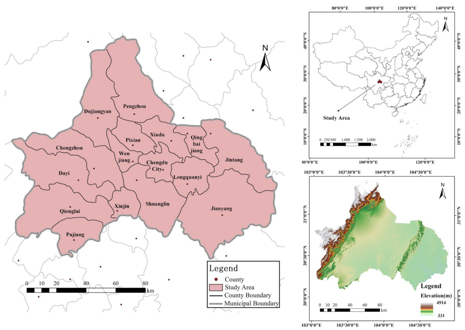
Contemporarily, the majority of studies in terms of urbanization and ecosystem services in China are concentrated on the central cities of the socially and economically developed regions located in eastern and central China. With the continuous acceleration of urbanization in Chengdu, a large decline in ecosystem service functions of urban ecosystems has been expected. This study evaluated and predicted the impact of the land use land cover changes on the urban ecosystem services in Chengdu city. The objectives of this study are: (1) detecting major drivers of the changes in land utilization categories; (2) calculating and predicting the ecosystem services value (ESV) by 2033; (3) combining with population and economy indicators to analyze the driving forces of the changes in ESV. Our results are expected to provide quantitative information which will assist in making decisions on the protection of natural environmental elements and enhancing urban sustainability in Chengdu, as well as providing insights into other cities with similar characteristics globally.

2. Data and Methods

2.1. Overview of Studied Area

Chengdu, (102°54′~104°53′E, 30°05′~31°26′N), is located on western Sichuan Plain in central Sichuan Province, China. Its terrain slopes from the northwest to the southeast, and the surface altitude varies from 331 m to 4914 m, showing the characteristics of high altitude in the northwest and low altitude in the southeast. Chengdu is adjacent to Deyang in the northeast, Neijiang in the southeast, Ya’an in the southwest, and Aba Tibetan and Qiang Autonomous Prefecture in the northwest. Western Chengdu is a marginal area of Sichuan Basin, which is dominated by steep hills and mountains. Eastern Chengdu is mainly composed of plains, platforms and some low mountains and hills, which is the heartland of Chengdu Plain. The maximum distance from east to west is 192 km, and the maximum distance from north to south is 166 km. Chengdu covers a total area of 12,400 km². The overall schematic diagram of the studied area is shown in Figure 1.

2.2. Data Source and Preprocessing

2.2.1. Data Source

The data sources used in this study were remote sensing image data and socioeconomic data. The remote sensing image data were Landsat 8 OLI and Landsat 7 ETM + images, obtained from the United States Geological Survey EarthExplorer website (https://earthexplorer.usgs.gov/). As three Landsat scenes are needed to cover the entire city of Chengdu, 12 Landsat images in total (three each from 2003, 2007, 2013 and 2018) were downloaded, and the specific information is given in

Table 1. Remote sensing image information.

Time	Line and Column Number	Sensor Type	Imaging Date
2003	129,039	Landsat 7 ETM+	27 January 2003
	130,038	Landsat 7 ETM+	19 February 2003
	130,039	Landsat 7 ETM+	19 February 2003
2007	129,039	Landsat 7 ETM+	19 September 2007
	130,038	Landsat 7 ETM+	19 April 2007
	130,039	Landsat 7 ETM+	19 April 2007
2013	129,039	Landsat 8 OLI	20 April 2013
	130,038	Landsat 8 OLI	17 August 2013
	130,039	Landsat 8 OLI	17 August 2013
2018	129,039	Landsat 8 OLI	18 April 2018
	130,038	Landsat 8 OLI	15 August 2018
	130,039	Landsat 8 OLI	19 January 2018

. Moreover, the main data of the average purchasing price of grains were from statistical data in the China Yearbook of Agricultural Price Survey (compiled by the National Bureau of Statistics, http://www.stats.gov.cn/), and the socioeconomic data for the driver analysis were from the Statistical Yearbooks of Chengdu from 2003 and 2018 (on the sharing platform of China Statistical Yearbook, https://www.yearbookchina.com/).

Landsat Level1T data were selected for the experiment, which have been corrected by system radiation and ground control points, and topographic correction via digital elevation model (DEM). To take advantage of Landsat’s rich spectral information, the ENVI5.3 FLAASH Atmospheric Correction Module was used to complete atmospheric correction.

2.2.2. Workflow of Data Processing

The overall processing process of the study is shown in Figure 2.

Combining the image and inventory data, the overlay analysis tool in the spatial analysis function of ArcGIS 10.3 software was used to intersect the current status maps of Chengdu’s land use types in 2003 and 2018. Based on the spectral response characteristics of each band, the Gram–Schmidt fusion method was used for image fusion processing. Considering that a Support Vector Machine (SVM) has good generalization ability, especially in a small sample training set, it can achieve much better results than other algorithms. The SVM with radial basis function was used to classify the images. We analyzed and predicted land use/cover in Chengdu to derive the ecosystem value.

(1)

Interpretation of remote sensing images

Pansharpening of the remote sensing images was carried out using the Gram–Schmidt Pan approach to obtain remote sensing image data with a spatial resolution of 15 m. The pansharpened images were mosaicked and then the study area was divided into four different sample plots. Next, according to the principle of simple random sampling, sample (training) data were collected from the remote sensing images for five land use/land cover categories: cultivated land, forest land, water area, construction land and unused land, and the training sample was evenly distributed on the remote sensing image. These training data were used to train a support vector machine classifier to generate a map of the study area, and man–machine interactive revisions were made to the categorized results to obtain the categorized land utilization map of the four sample plots in the end.

In the end, the categorized land utilization maps of the four sample plots were mosaicked into a grid map layer to produce the 2003, 2007, 2013 and 2018 categorized land utilization maps of Chengdu, as shown in Figure 3, and to obtain the area of different categories of land utilization.

While considering the high spatial resolution of pansharpened Landsat images, the validation data can be directly obtained by visual interpretation combined with field investigation and Google Earth’s high-resolution image.

For image 2003, 184 farmland verification samples, 195 forest land verification samples, 176 water area verification samples, 174 construction land verification samples and 126 unused land verification samples were randomly acquired by manual visual interpretation and Google Earth’s high-resolution image. A total of 202 farmland verification samples, 192 forest land verification samples, 180 water area verification samples, 178 construction land verification samples and 138 unused land verification samples were randomly acquired by manual visual interpretation and Google Earth’s high-resolution image for image 2007.

For experimental image 2013, 165 farmland verification samples, 188 forest land verification samples, 177 water area verification samples, 171 construction land verification samples and 141 unused land verification samples were randomly acquired by manual visual interpretation and Google Earth’s high-resolution image. A total of 172 farmland verification samples, 173 forest land verification samples, 211 water area verification samples, 196 construction land verification samples and 141 unused land verification samples were randomly acquired by manual visual interpretation and Google Earth’s high-resolution image for image 2018.

It can be obtained through the statistical calculation that the overall accuracy of image 2003 is 92.5%, and the Kappa coefficient is 0.821. Table 1 shows the specific results. The overall accuracy of image 2007 is 93.6%, and the Kappa coefficient is 0.856.

Table 2. Natural service function value coefficients. (CNY/hm²).

Function Type	Service Type	Farmland	Forest Land	Water	Construction Land	Unused Land	Total
Provisioning services	Food production	1735.00	386.86	1250.45	0.00	7.82	3380.12
	Raw material production	390.77	660.39	359.50	0.00	23.45	1434.11
	Supply of water resources	2047.61	355.60	12,957.79	0.00	15.63	11,281.40
Regulation services	Gas regulation	1391.13	2262.53	1203.56	0.00	101.60	4958.82
	Climatic regulation	734.64	6279.60	3579.41	0.00	78.15	10,671.81
	Environment purification	218.83	1989.00	8675.00	−3955.50	320.43	7247.75
	Hydrological regulation	2344.59	4591.50	159,807.52	−9015.20	187.57	157,915.98
Support services	Soil conservation	812.79	2758.81	1453.65	0.00	117.23	5142.48
	Maintenance of nutrient circulation	250.09	211.01	109.41	0.00	7.82	578.33
	Biodiversity	265.72	2508.72	3985.81	0.00	109.41	6869.66
	Total	6095.94	22,004.01	193,382.10	−12,970.70	969.10	209,480.46

shows the specific results. The overall accuracy of image 2013 is 91.7%, and the Kappa coefficient is 0.816.

Table 3. Areas and changes of different land use types in Chengdu from 2003 to 2018.

Land Use Type	2003		2018		Change
	Area (hm2)	Percentage (%)	Area (hm2)	Percentage (%)	Differential (hm2)	Range (%)	Dynamic Degree (%)
Farmland	604,408.01	42.33	370,411.90	25.94	−233,996.11	−38.71	−2.58
Forest land	711,379.31	49.82	703,435.95	49.26	−7943.35	−1.12	−0.07
Water	28,948.07	2.03	21,298.50	1.49	−7649.57	−26.43	−1.76
Construction land	67,327.99	4.72	297,448.65	20.83	230,120.66	341.79	22.79
Unused land	15,829.94	1.11	35,298.32	2.47	19,468.37	122.98	8.20

shows the specific results. The overall accuracy of image 2018 is 90.7%, and the Kappa coefficient is 0.834.

Table 4. Transfer matrix of land use change in Chengdu from 2003 to 2018.

Land Use Type		2018
		Farmland (hm2)	Forest Land (hm2)	Water (hm2)	Construction Land (hm2)	Unused Land (hm2)	Total (hm2)
2003	Farmland	9066.98	6030.11	1794.78	50,078.50	357.62	604,408.01
	Forest land	267,606.41	143,517.76	5113.31	167,887.60	20,282.94	711,379.31
	Water	85,141.76	541,492.02	4513.77	66,972.35	13,259.41	28,948.07
	Construction land	3860.19	5848.48	281.39	4733.86	1106.03	67,327.99
	Unused land	4736.56	6547.58	9595.26	7776.35	292.32	15,829.94
	Total	370,411.90	703,435.95	21,298.50	297,448.65	35,298.32	1,427,893.31

shows the specific results.

(2)

Analysis of changes in land utilization categories

The dynamic degree of land utilization in Chengdu from 2003 to 2008 was first calculated with the area data of different categories of land utilization to describe the dynamic changes in land utilization categories in the studied region (Figure 3). Then, the land use transfer matrix in the period of 2003–2018 was calculated to describe the conversion of land utilization categories from the beginning to the end of the study period. In the end, we used the forecasting method to predict the area of different categories of land utilization in Chengdu by 2033.

The ESV of Chengdu was calculated from three aspects, namely, different categories of land utilization, different service value types of the ecological system, and different districts and counties under Chengdu. Then, the ESV by 2033 was estimated by using the area of different categories of land utilization in Chengdu by 2033, predicted with the forecasting method.

(3)

Analysis on drivers for changes in ESV

Population and economic indicators were then introduced to establish the linear regression model between the ESV and the socioeconomic factor with the stepwise linear regression approach.

2.3. Study Methods

2.3.1. Land Use Analysis Method

(1)

Dynamic degree of land use

The dynamic degree of land use can be used to describe the dynamic changes of land use types in a certain studied area, and its essence is the area change of a certain land use type between the end and the beginning of this study [31]. The method for calculating the dynamic degree of land use is as follows:

$$D_s=\frac{S_2-S_1}{S_1}\times \frac{1}{T}\times 100\%$$

(1)

where D_s is the single land use dynamics; S₁ and S₂ are areas of a certain land use type at the beginning and end of this study (ha); T is the time interval from the beginning to the end of this study (a).

(2)

Land use transition matrix

The land use transition matrix is used to describe the transition of land use types from the beginning to the end of this study. Through this matrix, the transition direction and amount of land use can be clearly depicted. In actual operation, it can be obtained by the intersection of the land use maps of the beginning and end of this study. Its specific mathematical form is as follows:

$$S_{ij}=\left[\begin{array}{cccc}{S}_{11}& S_{12}& \dots & S_{1n}\\ S_{21}& S_{22}& \dots & S_{2n}\\ ⋮& ⋮& ⋮& ⋮\\ S_{n1}& S_{n2}& \cdots & S_{nn}\end{array}\right]$$

(2)

where S_ij is the area transited from a certain land use type i to another land use type j from the beginning to the end of this study (hm²); n is the number of land use types divided in the studied area, n = 5 in this study.

(3)

Markov forecast method

The Markov forecast method is based on the Markov chain, which forecasts the changes at various moments (periods) in the future according to the current state of the event. This method requires “no aftereffect” in the random process, that is, during the development of the event, each state transition is only related to the state at the previous moment, and has nothing to do with the state in the past [32,33,34]. Therefore, this forecast method is widely used in this study of land use change. Its specific calculation method is as follows:

$$\pi (k)=\pi (k-1)\times P$$

(3)

where π(k) is the probability of being in a certain land use state at the time k; π(k−1) is the probability of being in a certain land use state at the time k−1; P is the state transition probability matrix, and its specific mathematical form is as follows:

$$P=\left[\begin{array}{cccc}{P}_{11}& P_{12}& \dots & P_{1n}\\ P_{21}& P_{22}& \dots & P_{2n}\\ ⋮& ⋮& ⋮& ⋮\\ P_{n1}& P_{n2}& \cdots & P_{nn}\end{array}\right]$$

(4)

$$P_{ij}=\frac{C_{i-j}}{S_i}$$

(5)

where n is the number of states; P_ij is the state transition probability from the state i to the state j; C_i−j is the area transited from a certain land use type i to another land use type j during the time range of this study (hm²); S_i is the area of a certain land use type i at the beginning of this study (hm²). In addition, the state transition probability matrix satisfies the following properties:

$$\left\{\begin{array}{cc}0\le P_{ij}\le 1& (i,j=1,2,\dots ,n)\\ {\displaystyle \sum _{j=1}^n{P}_{ij}}=1& (i=1,2,\dots ,n)\end{array}\right.$$

(6)

2.3.2. Method for Calculating Natural Service Function Value

Based on part of the results of Costanza’s evaluation of the global ecosystem service value in 1997, Fu et al. synthesized the results of an ecological questionnaire survey of Chinese professionals, established a table of service equivalent factors per unit area of China’s terrestrial ecosystem, and obtained a method for calculating natural service function value that meets the actual conditions in China [35,36,37,38]. That is, 1/7 of the economic value of the annual natural grain output of 1 hm² farmland with national average yield is first defined as 1 equivalent factor of ecosystem service value. The specific calculation method is as follows:

$$V_0=\frac{1}{7}\times \frac{{\displaystyle \sum _{i=1}^n\frac{y}{M}}}{n}\times d$$

(7)

where V₀ is the unit ecosystem service value (CNY), y is the total grain output (kg); M is the total grain-sown area (hm²); n is the time interval from the beginning to the end of this study (a); d is the purchase price of grain (CNY/kg). In this study, the average purchase price of grain in Chengdu in 2010 was 1.82 CNY/kg.

Then, based on the actual classification of land use types in Chengdu, the equivalent factors of the four land use types of farmland, forest land, water and unused land were revised by referring to the improvement results of Shoyama et al. on the value equivalent factor per unit area [39]. Among them, farmland corresponds to fields (take the average value of equivalent factors of dry land and paddy field), forest land corresponds to the average value of forest and grassland (broad-leaved forest, grassland, shrub and grass, and meadow), water corresponds to water area (water system), and unused land corresponds to desert (take the average value of desert and bare land).

Since the effect of construction land on ecosystem service functions is not considered in the above study, it actually has a certain weakening effect on the natural service function value. Therefore, the table of ecological service value per unit area of different land use types in the Miyun Reservoir catchment area obtained by Zheng Kenter et al. and the study results of the biomass factor of farmland ecosystems in different provinces in China obtained by Rodríguez-Ortega et al. are referred to in this study [40,41,42,43], and amended to obtain the ecosystem service value of the construction land in Chengdu.

Then, the natural service function value corresponding to the above-mentioned 1 equivalent factor is multiplied by the ecosystem service equivalent factor per unit area of the first four types of land use in turn to obtain the natural service function value coefficients of Chengdu, as shown in Table 2.

Finally, the specific natural service function service value can be calculated according to the following formula:

$$V_N={\displaystyle \sum _{i=1}^n{\displaystyle \sum _{j=1}^m{A}_i\times K_{ij}}}$$

(8)

where V_N is the total natural service function value of Chengdu (CNY); n is the land use type; m is the specific function type, m = 10 in this study; A_j is the area of the land use type i (hm²); K_ij is the coefficient of ecosystem service value j of land use type i (CNY/hm²).

2.3.3. Social Factor Driver Analysis Method

(1)

Selection of driver factors

The variation in ESV is affected and limited by many natural and social factors. For urban areas with a highly concentrated population and economic activities, the social factor is the main driver for variation in its ecological system. According to relevant studies and in combination with the actual urban conditions of Chengdu, 15 population and economic indicators were used for the driver analysis, where the population indicators included the regional total population X₁, the non-agricultural population X₂ and the urbanization rate X₃. The economic indicators included the regional GDP X₄, the per capita GDP X₅, the per capita cash income of urban residents X₆, the primary industry output X₇, the secondary industry output X₈, the third industry output X₉, the grain yield X₁₀, the total real estate investment X₁₁, the gross agricultural production growth rate X₁₂, the gross forest production growth rate X₁₃, the gross livestock production growth rate X₁₄ and the gross fishery production growth value X₁₅.

(2)

Driver analysis method

The urbanization rate is the first driving factor for the ESV. This indicator is a population statistical indicator for measuring the urban development of a region, i.e., the proportion of urban population in total population (including agricultural and non-agricultural populations). Urbanization is a comprehensive and complicated changing process and involves the migration and moving of population, changes in production and living methods, changes in industrial and economic structures, etc.

In the driver analysis, software SPSS24.0 was used to establish the correlation analysis and the regression equation of the indicators selected to study the impacts of the social factor on ESV variation. The correlation analysis was to conduct double-variable analyses on the ESV and social factor indicators of the studied region from 2003 to 2018 to take out factors of a low correlation. On the basis of the correlation analysis, the stepwise regression was performed with the socioeconomic factor from 2003 to 2018 as the independent variable and the ESV as the dependent variable to establish the linear regression equation between the ESV and the socioeconomic factor. The driving mechanism model of the linear regression equation is as follows:

$$Y_m=aF(x_n)+\beta$$

(9)

where: Y_m is the ESV; x_n represents the social driver; α and β are the model coefficients.

3. Results

3.1. Cclassification Accuracy Assessment

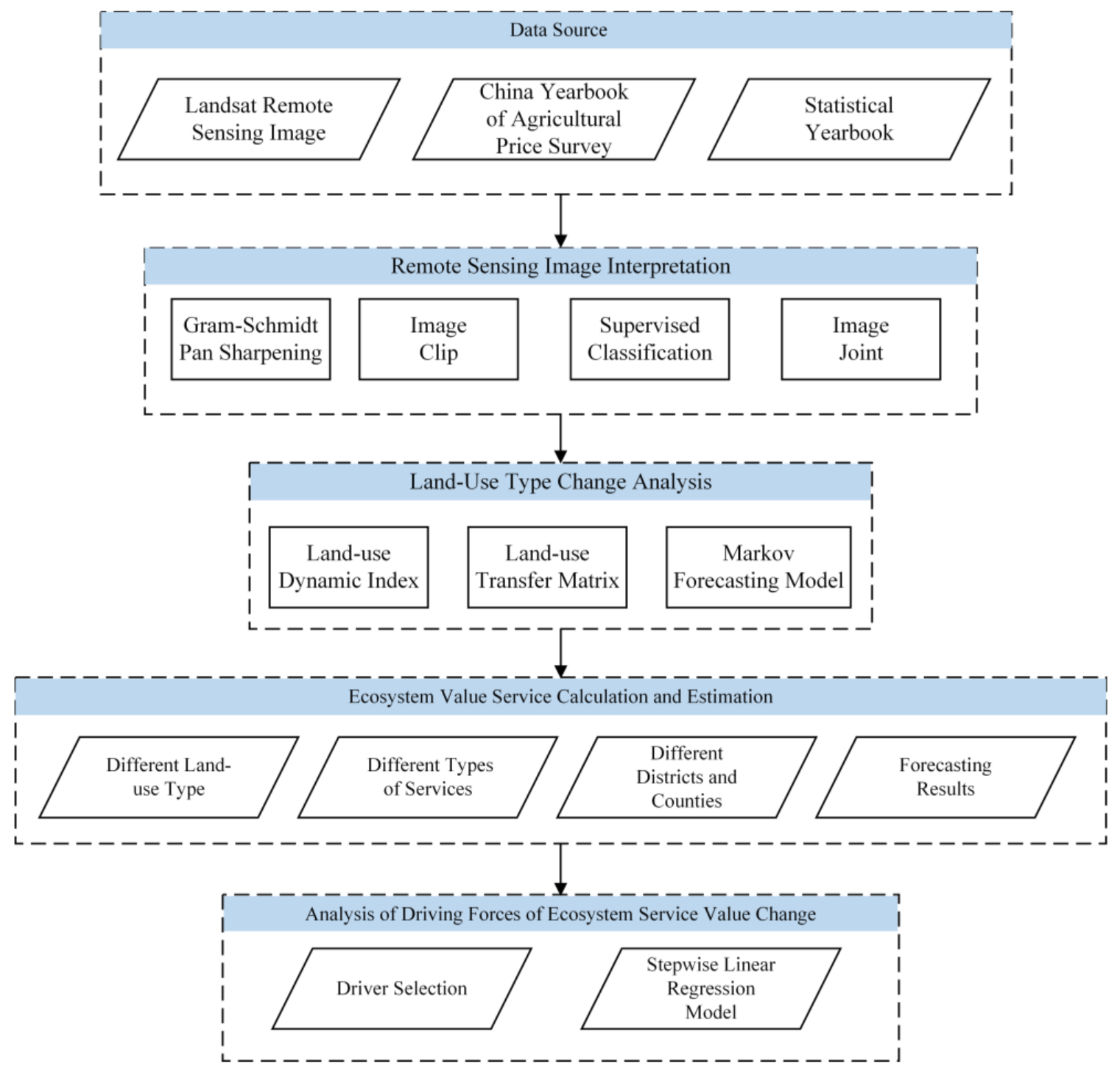
There are many methods for evaluating the landslide feature extraction results. The Confusion Matrix is used to verify the accuracy of the interpretation model, in accordance with the quantitative research needs in this paper [44]. We validated the accuracy of our classification against a high-resolution image obtained from the Google Earth web-based portal. The Kappa coefficient was used in the monitoring and categorization of the remote sensing images. We obtained a general Kappa coefficient over 0.80, implying that the remote sensing interpretation effect was good, and the data can be used to analyze the actual changes in land utilization in Chengdu. More information about the selected training sample, verification sample and the confusion matrix after classification are shown in the Appendix A. Due to the large number of confusion matrices (a total of 16), the Appendix A only shows the confusion matrix of the sample plot 1 in 2003.

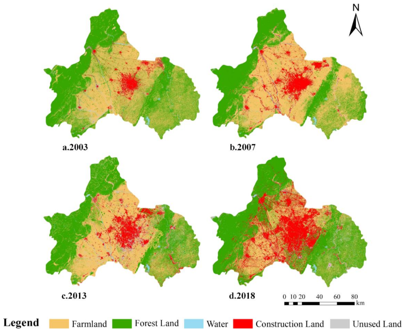
3.2. Analysis of Land Use Changes in Chengdu

Seen from Table 3, the land use types in Chengdu are mainly farmland and forest land, which account for 92.15% and 72.4% of the total area in 2003 and 2018, respectively.

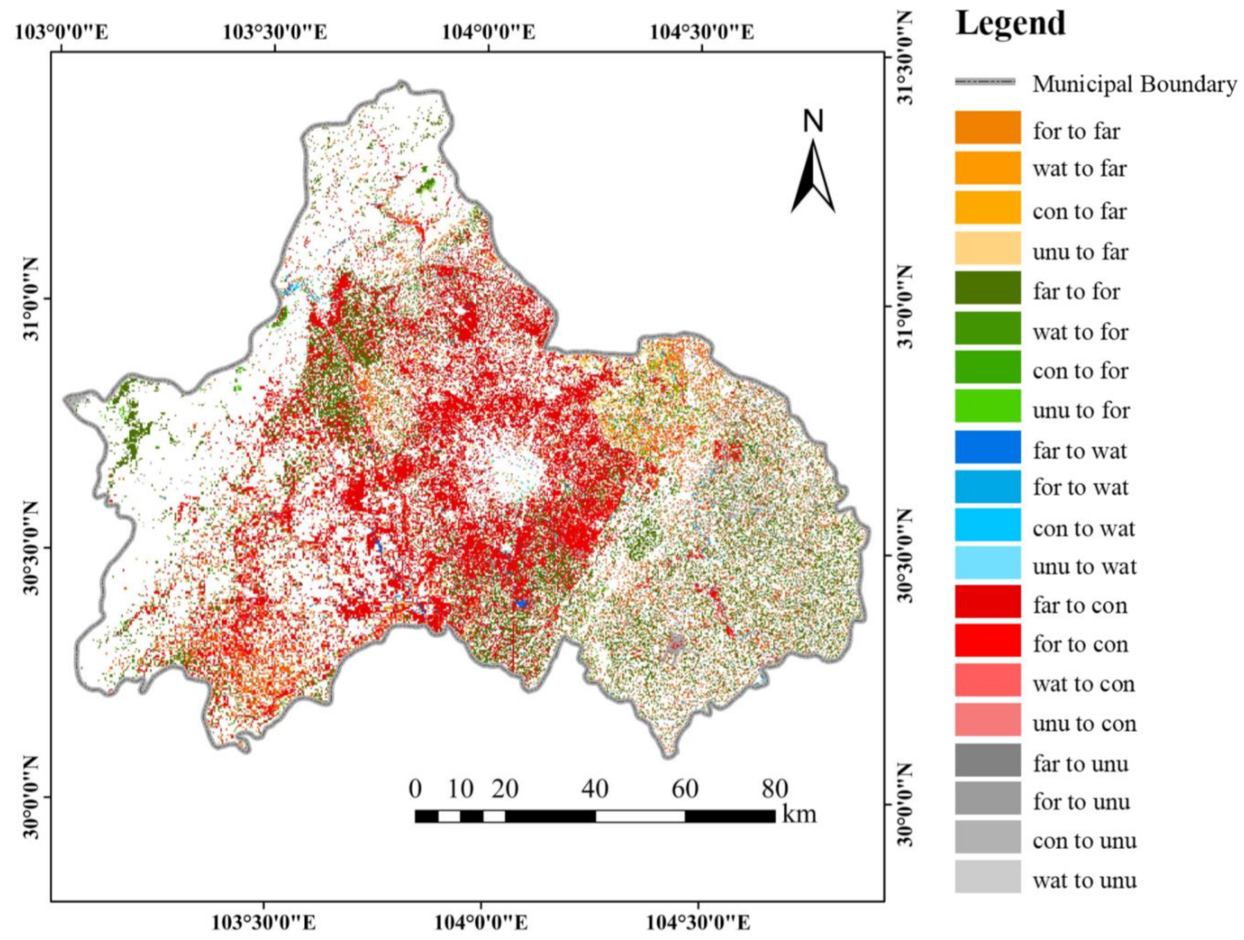
In order to study the area transition between the five land use types in Chengdu after obtaining the areas of various land use types, we calculated the transition matrix of the five land use types in Chengdu and their spatial transition within this study time frame, as shown in Table 4 and Figure 4.

From 2003 to 2018, the areas of land use types in Chengdu changed significantly, mainly concentrated in the decrease in farmland and the increase in construction land. Among them, the farmland decreased by 233,996.11 hm², with a change rate of 38.71%, the dynamic degree was 2.58%, and the transited-out area reached 336,801.60 hm², most of which was transited to construction land and forest land; the transited-out areas were 167,887.60 hm² and 143,517.76 hm², respectively, accounting for 92.46% of the total transited-out area. In terms of spatial changes, the spatial changes of farmland were mainly concentrated in the central area of entire Chengdu. A large amount of farmland was transited into construction land, presumably because this part of the area was flat and suitable for agricultural development.

The following types are forest land and water, and their areas decreased by 47,943.35 hm² and 7649.57 hm², respectively, by 6.74% and 26.43%, and the dynamic degrees were 0.45% and 1.76%. Among the transited-in area of forest land, most of it was transited from farmland, and the transited-in area reached 143,517.76 hm², which accounted for 88.62% of the total transited-in area. Most of the transited-out part of the water is construction land, with an area of 7776.35 hm², accounting for 40% of the total transited-out area, which was mainly distributed in northern Chengdu.

The area of construction land in Chengdu increased sharply, and this area in 2018 was about four times that of 2003. The huge increase in the area of construction land was mainly transited-in from farmland and forest land, with transited-in areas of 167,887.60 hm² and 66,972.35 hm², respectively. In terms of spatial distribution, changes in the spatial distribution of construction land were scattered in the fringe area of the central region and the northeastern region, similar to the conclusion drawn by Sannigrahi et al. [45].

The unused land increased by 19,468.38 hm², a ratio of 122.98%, and the dynamic degree was 8.20%. Among it, the transition from farmland and forest land accounted for the vast majority, accounting for 98.1% of the total transited-in area. In terms of spatial changes, due to the rapid development of the city, although a large amount of unused land in central Chengdu has been transited into construction land, it is speculated that the central area is flat and suitable for the promotion of urbanization. As a result, a large amount of farmland has been shelved and forest land has been cut down to be used as a reserve for construction land.

3.3. Estimation of Ecosystem Service Value in Chengdu

Seen from

Table 5. Ecosystem service value of different land use types of Chengdu from 2003 to 2018.

Land Use Type	Natural Service Function Value				Change Rate (%)
	2003	2007	2013	2018	2003–2007	2007–2013	2013–2018	2003–2018
Farmland	36.84	44.82	36.69	22.58	21.64	−18.12	−38.47	−38.71
Forest land	156.53	116.81	131.86	154.78	−25.37	12.88	17.39	−1.12
Water	55.98	50.61	78.23	41.19	−9.59	54.57	−47.35	−26.43
Construction land	−8.73	−16.65	−17.97	−38.58	−90.68	−7.89	−114.75	−341.79
Unused land	0.15	0.07	0.46	0.34	−53.90	548.01	−25.35	122.98
Total	240.78	195.66	229.28	180.31	−18.74	17.18	−21.36	−25.11

Note: the unit of natural service function value is CNY 10⁸.

, from 2003 to 2018, the overall natural service function value in Chengdu showed a decreasing trend, from CNY 2.4078 × 10¹⁰ in 2003 to CNY 1.6632 × 10¹⁰ in 2018, a decrease of CNY 7.446 × 10⁹, with a change rate of 30.92%. Among the five land use types, forest land accounts for the largest proportion of the natural service function value, accounting for more than 50% of the total ecological service value from 2003 to 2018, followed by water, and finally farmland. In the past 16 years, the natural service function values of forest land, farmland, water, and construction land showed a decreasing trend, and the project of returning farmland to forest is coordinated with regional economic development [46,47,48]. Among them, construction land has always played a negative role for the natural service function value. From 2003 to 2018, the ecological value of construction land decreased by 401.20%, indicating that the area of construction land in Chengdu increased significantly from 2003 to 2018, and the ecological environment of Chengdu was more severe. The service value of unused land increased by 122.98%. However, due to the small area of unused land, its natural service function value had little effect, accounting for less than 1% of the total ecological service value.

From the perspective of the specific types of natural service functions, as shown in

Table 6. Various ecosystem service values of Chengdu from 2003 to 2018.

Function Type	2003		2007		2013		2018
	Value	Per (%)	Value	Per (%)	Value	Per (%)	Value	Per (%)
Food production	13.60	5.65	15.14	7.74	13.27	5.79	9.42	5.22
Raw material production	7.17	2.98	6.47	3.31	6.47	2.82	6.18	3.43
Supply of water resources	−6.09	−2.53	−9.77	−5.00	−4.95	−2.16	−2.32	−1.29
Gas regulation	24.87	10.33	22.56	11.53	22.47	9.80	21.36	11.85
Climatic regulation	50.16	20.83	39.68	20.28	43.54	18.99	47.68	26.45
Environment purification	15.37	6.38	9.38	4.80	11.42	4.98	5.00	2.77
Hydrological regulation	87.06	36.16	71.88	36.74	93.88	40.95	48.27	26.77
Soil conservation	24.98	10.37	21.01	10.74	22.07	9.63	22.77	12.63
Maintenance of nutrient circulation	3.05	1.26	2.99	1.53	2.82	1.23	2.44	1.35
Biodiversity	20.62	8.57	16.32	8.34	18.30	7.98	19.52	10.83
Total	240.78	100.00	195.66	100.00	229.28	100.00	180.31	100.00

Note: the unit of ecosystem service value is CNY 10⁸, per means percentage.

, the values of food production, environment purification and hydrological regulation functions decreased significantly from 2003 to 2018. In 2018, they decreased by 31.91%, 82.95% and 50.08%, respectively, compared with that in 2003. The water supply function is the only one showing an increasing trend, with an increase of CNY 3.63 × 10⁸, which is speculated to be related to the decrease in the area of farmland and the decrease in water consumption. However, the water supply service function still has a negative effect on the service value, which indicates that the situation in Chengdu is still quite severe in terms of water supply. In terms of specific value, the service value generated by the hydrological regulation function was the largest from 2003 to 2018, which was CNY 8.706 × 10⁹, CNY 9.601 × 10⁹, CNY 9.362 × 10⁹, and CNY 4.283 × 10⁹ in order. The water supply function value was the smallest, which was CNY −6.09 × 10⁸, CNY −6.27 × 10⁸, CNY −5.24 × 10⁸, and CNY −2.46 × 10⁸, respectively.

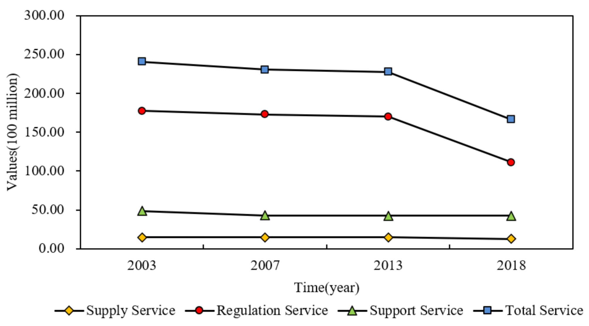
As shown in Figure 5, in respect of the three ecosystem service categories, the gross value showed an apparent downtrend and decreased from CNY 2.4078 × 10¹⁰ in 2003 to CNY 1.6632 × 10¹⁰ in 2018, a drop as large as 30.92%. The regulating service value took up a large portion of the gross value, accounting for 72.58% on average. Additionally, the decreasing trend of the regulating service value was in line with the downtrend of the gross value, which decreased from CNY 1.7745 × 10¹⁰ in 2003 to CNY 1.1107 × 10¹⁰ in 2018, a drop of 37.41%, meaning the regulating service value played a leading role in the ecosystem gross service value. The proportions of support service and supply service values in the gross value were small, accounting for 20.79% and 6.63% on average, respectively, and they decreased slowly by 12.57% and 13.36% from 2003 to 2018, respectively.

Seen from

Table 7. Natural services function values in all districts of Chengdu from 2003 to 2018.

Study Area	Ecosystem Service Value								Change Rate (%)
	2003	seq	2007	seq	2013	seq	2018	seq	2003–2018
Chengdu City	−0.80	16	−0.86	16	0.08	16	−2.85	16	−257.86
Chongzhou	19.76	7	19.16	7	19.33	7	10.58	7	−46.46
Dujiangyan	23.22	4	23.03	4	23.61	4	19.09	4	−17.80
Jintang	21.05	6	21.00	6	20.97	6	20.02	2	−4.92
Pengzhou	26.32	3	23.16	3	23.82	3	19.16	3	−27.19
Pujiang	13.77	8	11.79	9	6.70	10	5.56	9	−59.64
Qionglai	28.49	2	27.12	2	24.82	2	15.95	6	−44.03
Wenjiang	3.70	13	2.80	12	3.07	14	1.11	13	−70.04
Xinjin	4.91	11	8.44	11	7.66	9	1.88	12	−61.70
Dayi	22.86	5	22.25	5	22.98	5	16.63	5	−27.27
Janyang	44.17	1	41.23	1	46.05	1	46.99	1	6.38
Longquan	8.94	10	8.55	10	5.96	11	3.53	10	−60.56
Pixian	3.58	14	3.40	14	2.88	15	−1.07	14	−129.98
Qingbaijiang	3.20	15	3.01	15	4.41	12	3.28	11	2.28
Shuangliu	13.39	9	12.96	8	11.39	8	8.48	8	−36.70
Xindu	4.15	12	3.41	13	3.63	13	−2.00	15	−148.18
Total	240.74	//	230.45	//	227.37	//	166.32	//	−30.91

Note: the unit of ecosystem service value is CNY 10⁸, seq means sequence.

, from 2003 to 2018, Jianyang had the highest natural service function value, with the lowest in downtown Chengdu. Among the changes in service value, in the sixteen areas, only Xinjin had an increase in ecological service value from 2003 to 2007, an increase of 71.89%. The values of other areas were decreasing, and among such areas, downtown Wenjiang had the largest change rate, up to 24.32%. From 2007 to 2013, the natural service function value increased in downtown Chengdu, Chongzhou, Dujiangyan, Pengzhou, Wenjiang, Dayi, Jianyang, Qingbaijiang, and Xindu. Downtown Chengdu had the largest change rate of increase at 109.29%, and Chongzhou had the smallest at 0.92%. Pujiang and Longquan showed a decrease in values. From 2013 to 2018, only Jianyang showed an increase in natural service function value, by 2.04%, and the values of the remaining areas decreased. Downtown Chengdu showed the largest change rate of decrease, up to 3678.46%. From 2003 to 2018, the natural service function value showed an increasing trend in Jianyang and Qingbaijiang, with increase change rates of 6.38% and 2.28%, respectively, while that of remaining areas was decreasing.

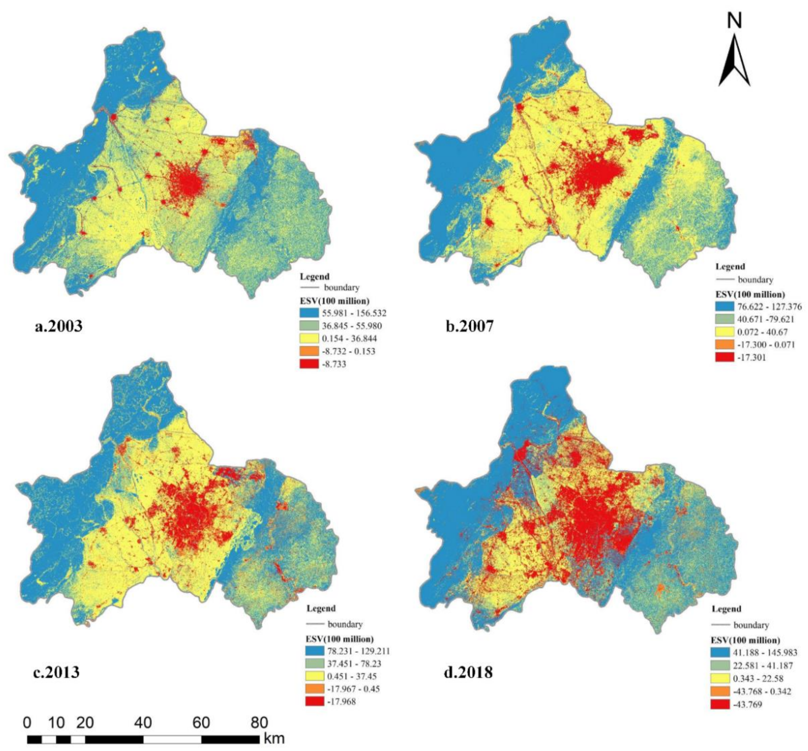
The natural breakpoint method was used to classify the ecosystem service value, which is a statistical method to classify and categorize the data according to the statistical distribution of values, and it maximizes the difference between classes. As shown in Figure 6, the ESV of Chengdu from 2003 to 2018 presented a circled characteristic in terms of spatial distribution, i.e., being lower at the center and higher at the periphery, and varied in different directions. The low-value concentration areas have expanded structurally in the last 15 years, i.e., urban roads were taken as low-value extension routes to spread to the districts and counties in the 2nd circle, such as Longquanyi, Shuangliu, etc. In the meantime, the service values were gradually fixed in a circular distribution and, with the downtown area as the core, derived from the “low-medium-high-high” to the “low-low-medium-high” gradient structure. This structure was deployed with the main urban development direction as the axis and with urban–rural fringes as the fast structural variation zones, showing the fringe effect in the evolution process of the urban ecosystem.

As shown in

Table 8. Forecast of the ecosystem service value of Chengdu in 2033.

Land Use Type	Area (hm2)	Percentage (%)	Ecosystem Service Value
Farmland	278724.77	19.52	16.99
Forest land	632413.95	44.29	139.16
Water	25844.87	1.81	49.98
Construction land	463922.54	32.49	−60.17
Unused land	26987.18	1.89	0.26
Total	1427893.31	100	146.21

Note: the unit of ecosystem service value is CNY 10⁸.

, according to the Markov forecast method, the area of each land use type in Chengdu in 2033 can be forecast, and it is forecast that the total natural service function value in Chengdu in 2033 will be CNY 1.4621 × 10¹⁰, a decrease of CNY 3.41 × 10⁵ compared to that in 2018.

3.4. Analysis on Drivers for Changes in ESV

The regression model of drivers for changes in the ESV of Chengdu was obtained through stepwise linear regression, as shown in

Table 9. Chengdu ecosystem service value regression model.

Ecosystem Service Value	Regression Model
Total service value	$Y=-300.683X_1-2.724\times {10}^8{X}_3-1.465\times {10}^4{X}_5-4.380\times {10}^{10}$
Supply services value	$Y_1=-7.906X_1-7.162\times {10}^6{X}_3-385.228X_5+1.996\times {10}^9$
Regulation services value	$Y_2=-269.445X_1-2.441\times {10}^8{X}_3-1.312\times {10}^4{X}_5+3.566\times {10}^{10}$
Support services value	$Y_3=-23.332X_1-2.114\times {10}^7{X}_3-1.137\times {10}^3{X}_5+6.146\times {10}^9$

below. The regression model indicated that, among the 15 social driving factors selected in the study, the ESV and regional total population of Chengdu X₁ (population factor), the urbanization rate X₃ (population factor) and the per capita GDP X₅ (economic factor) showed an apparent negative correlation.

The urbanization of Chengdu has developed rapidly in recent years, and the urban development spatial strategy principally expressed as “advancing in the east, expansion in the south, controlling in the west, reform in the north and optimization in the center” was formally proposed in April 2017. The fast urbanization process is generally accompanied by a surge in urban construction lands and the loss of large areas of farmland and forest ecosystems, which will certainly result in a reduction in the ESV.

The per capita GDP is the second driving factor for the ESV. This indicator is used to calculate the regional GDP realized in a calculation period (generally a year) against the gross population of the region to present the regional economic conditions in a more objective way. The average growth rate of the per capita GDP of Chengdu in the last 15 years was around 13%. Fast economic development is also accompanied by the fast consumption of resources and strong changes in the categories of land utilization, resulting in a decrease in ESV.

The regional total population is the third driving factor for the ESV. This indicator can reflect the consumption of ecological resources in a region. From 2003 to 2018, the total population of Chengdu was always maintained over 10 million and kept a growing trend. In general, the larger the population is, the more remarkable the consumption of various resources would be, thus reducing the ESV of the region.

4. Discussion

Chengdu is an important central city in western China and an important gateway hub for the “Belt and Road” and the Yangtze River Economic Belt. In this study, Chengdu is taken as an example, and its values of ecosystem services are estimated from the perspectives of natural ecology and social ecology, based on the remote sensing interpretation data of four phases of 2003, 2007, 2013 and 2018, and socio-economic data from 2003 to 2018. In addition, the Markov model is used to forecast Chengdu’s natural ecological service function value in 2033 and establish a unary linear regression model to analyze the driving effect of economy and population indicators in the social and ecological service function values. Unlike previous works, this study proposed methods to determine evaluation factors and evaluation systems to calculate the ecosystem service values of economically developed cities. Different conditions are set to analyze the development trend of functional areas. It not only enriches the study of ecological service functions theoretically, but also guides the construction of ecological cities.

Chengdu is located in the Sichuan Basin, it is cloudy all year round and there are few available images. In addition, Chengdu is located in the mid and low latitude region, and the seasonal variation of vegetation is relatively small. The experimental design did not consider the possible influence of annual change information on the results. The results of the accuracy test also show that the experiment has good accuracy and high reliability. A notable increase in forest land can be observed in the southeast region of Chengdu city, due, in part, to the revegetation program conducted by the local government, including the natural forest protection project and the cropland re-vegetation project. Accordingly, the synthetic project report, namely as the year book of forest resources and ecosystem services of Chengdu city, can help support this finding, which stated that the forest coverage increased by 39.1% during the past five years.

In terms of the estimation of natural service function value, the calculation method improved by Lyver on the successful study of Costanza et al. is mainly adopted in this paper. As for different land use types, in this method, 1/7 of the economic value of the annual natural grain output of 1 hm² farmland with national average yield is first defined as 1 equivalent factor of ecosystem service value to obtain the table of natural service function value coefficients. It is convenient and quick to calculate the natural service function value on this basis. However, it is necessary to correct the coefficients when studying different studied areas, considering the regional heterogeneity and the complexity of the ecosystem itself. In addition, since the impact of urban land use on natural service functions is not taken account in this method, the correlation coefficient is obtained in this paper by reversely modifying the data [49].

The Markov process can effectively forecast the future land use structure under the current land use change trend. However, land use is subject to multiple impacts such as national policies [50], human activities [51], natural disasters, and climate changes. The complexity and difficulty of forecasts are significant. This requires in-depth discussion and gradual improvement. In this paper, the significant increase in the area of construction land is only seen from the land use changes, while urbanization factors such as urban expansion are not further analyzed. Comprehensive analysis can be considered for urbanization factors such as farmland reduction, urban expansion, and changes in ecosystem service value.

5. Conclusions

In this paper, we deployed a detailed evaluation of ESV in the response of urbanization induced land-use/land-cover (LULC) change for the big city of Chengdu, China. Based on the land use data and socio-economic data interpreted by Landsat remote sensing products, the ecosystem service values during the 16 years from 2003 to 2018 are estimated from the perspectives of natural ecology and urban ecology. The natural service function value in Chengdu in 2033 is also forecast, and the driving effects of society and population indicators on the social service function value are analyzed. After taking out data with colinearity and with a low correlation with ecosystem services through relevant analyses, social indicators of a high correlation were used in the stepwise regression analysis of the ESV of Chengdu, and both the model and the related parameters to be estimated reached a remarkable level. Among the 15 social population and economic driving factors, the ESV and regional total population, the urbanization rate and the per capita GDP showed an apparent negative correlation. This indicates that the negative economic effect caused by urban development can be effectively mitigated through rationally adjusting the spatial distribution of industries, optimizing and upgrading the industrial structure and strengthening the control over construction lands. In this study, the relationship between LULC and ESV was explored using relatively coarse resolution Landsat satellite imageries. Although the table of ecological service value per unit area of China’s terrestrial ecosystems recently formulated by relevant researchers is adopted in this paper, the difference in the spatial distribution of value coefficients and quality factors suitable for this area still needs to be investigated and studied, and how to comprehensively consider the impact of urban ecosystems on natural service functions still needs further studies.